Transient Analysis of Large Markov Models with Absorbing

States using Regenerative Randomization

Juan A. CarrascoDepartament d’Enginyeria ElectronicaUniversitat Politecnica de Catalunya

Diagonal 647, plta. 908028 Barcelona, Spaincarrasco@eel.upc.edu

Technical report DMSD 99 2

Last revision: April 30, 2005appeared in reduced form in Communications in Statistics—Simulation and Computation

Abstract

In this paper, we develop a new method, called regenerative randomization, for the transientanalysis of continuous time Markov models with absorbing states. The method has the samegood properties as standard randomization: numerical stability, well-controlled computationerror, and ability to specify the computation error in advance. The method has a benign behaviorfor large t and is significantly less costly than standard randomization for large enough modelsand large enough t. For a class of models, class C, including typical failure/repair reliabilitymodels with exponential failure and repair time distributions and repair in every state with failedcomponents, stronger theoretical results are available assessing the efficiency of the method interms of “visible” model characteristics. A large example belonging to that class is used toillustrate the performance of the method and to show that it can indeed be much faster thanstandard randomization.

Index terms: Continuous time Markov chains, transient analysis, randomization, reliability, fault-tolerant systems.

1 Introduction

Homogeneous continuous time Markov chains (CTMCs) are frequently used for performance, de-pendability and performability modeling. The transient analysis of these models is usually signifi-cantly more costly than the steady-state analysis, and very costly in absolute terms when the CTMCis large. This makes the development of efficient transient analysis techniques for CTMCs a re-search topic of great interest. Commonly used methods are ODE (ordinary differential equation)solvers and randomization. Good recent reviews of these methods with new results can be foundin [17, 18, 26]. The randomization method (also called uniformization) is attractive because of itsexcellent numerical stability and the facts that the computation error is well-controlled and can bespecified in advance1. It was first proposed by Grassman [11] and has been further developed byGross and Miller [13]. The method is offered by well-known performance, dependability and per-formability modeling packages [2, 7, 8, 10]. The randomization method is based on the followingresult [15, Theorem 4.19]. Let X = {X(t); t ≥ 0} be a CTMC with finite state space Ω; let λi,j ,i, j ∈ Ω, i �= j be the transition rate of X from state i to state j, and let λi =

∑j∈Ω−{i} λi,j ,

i ∈ Ω be the output rate of state i. Consider any Λ ≥ maxi∈Ω λi and define the homogeneousdiscrete time Markov chain (DTMC) X = {Xk; k = 0, 1, 2, . . .} with same state space and initialprobability distribution as X and transition probabilities P [Xk+1 = j | Xk = i] = Pi,j = λi,j/Λ,i �= j, P [Xk+1 = i | Xk = i] = Pi,i = 1 − λi/Λ. Let Q = {Q(t); t ≥ 0} be a Poisson processwith arrival rate Λ (P [Q(t) = k] = e−Λt(Λt)k/k!) independent of X . Then, X = {X(t); t ≥ 0} isprobabilistically identical to {XQ(t); t ≥ 0} (we call this the randomization result). The DTMC X

is called the randomized DTMC of X with rate Λ. The CTMCX is called the derandomized CTMCof X with rate Λ.

Assume that a reward rate structure, ri ≥ 0, i ∈ Ω is defined over the state space of X. Thequantity ri has the meaning of “rate” at which reward is earned while X is in state i. Then, a usefulmeasure to consider is the expected transient reward rate ETRR(t) = E[rX(t)]. Using the factsthat X = {X(t); t ≥ 0} and {XQ(t); t ≥ 0} are probabilistically identical and that X and Q areindependent, we can express ETRR(t) in terms of the transient regime of X as

ETRR(t) =∑i∈Ω

riP [X(t) = i] =∑i∈Ω

ri

∞∑k=0

P [Xk = i]P [Q(t) = k]

=∞∑

k=0

∑i∈Ω

riP [Xk = i]e−Λt (Λt)k

k!=

∞∑k=0

d(k)e−Λt (Λt)k

k!, (1)

with d(k) =∑

i∈Ω riP [Xk = i]. Denoting by q(k) = (P [Xk = i])i∈Ω the probability row vectorof X at step k, q(k), k > 0 can be obtained from q(0) using

q(k + 1) = q(k)P, (2)

where P = (Pi,j)i,j∈Ω is the transition probability matrix of X .

1The computation error has two components: truncation error and round-off error; the truncation error can be madearbitrarily small, the round-off error will have a very small relative value due to the numerical stability of the method ifdouble precision is used. Rigorous bounds for the round-off error have been obtained in [12] under certain conditionsconcerning the values that transition rates can have and assuming a special method for computing Poisson probabilities.

1

In a practical implementation of the randomization method, an approximate value for ETRR(t),ETRRa

N (t), is obtained by truncating the summatory (1) so that N steps have to be given to X :

ETRRaN (t) =

N∑k=0

d(k)e−Λt (Λt)k

k!,

and, taking into account that 0 ≤ d(k) ≤ rmax = maxi∈Ω ri, the truncation error verifies

0 ≤ ETRR(t) − ETRRaN (t) ≤ rmax

∞∑k=N+1

e−Λt (Λt)k

k!.

A usual accuracy requirement is to limit the truncation error to a value ≤ ε. Then, N is chosen as

N = min{m ≥ 0 : rmax

∞∑k=m+1

e−Λt (Λt)k

k!≤ ε

}.

Stable and efficient computation of the Poisson probabilities e−Λt(Λt)k/k! avoiding overflows andintermediate underflows is a delicate issue and several alternatives have been proposed [4, 9, 16, 22].Our implementation of both standard randomization and regenerative randomization use the methoddescribed in [16, pp. 1028–1029] (see also [1]), which has good numerical stability.

For large models, the computational cost of the randomization method is roughly due to the Nvector-matrix multiplications (2). The truncation parameterN increases with Λt and, for that reason,Λ is usually taken equal to maxi∈Ω λi. Using the well-known result [27] that Q(t) has for Λt→ ∞an asymptotic normal distribution with mean and variance Λt, it is easy to realize that, for large Λtand ε � 1, the required N will be ≈ Λt. If one is interested in solving the model for values of tfor which Λt is very large, randomization will be highly inefficient. Consider, for instance, a CTMCdependability model of a fault-tolerant system with hot restarts having an exponential duration withmean 1 minute so that Λ is of the order of 1 min−1. For a time t = 1 year, Λt ≈ 525,600, makingrandomization very inefficient if X is large.

The randomization result can also be exploited to develop methods to compute more complexmeasures such as the distribution of the interval availability [28, 29, 33] and the performability[23, 25, 34, 35]. The performance of those methods also degrades as Λt increases.

Several variants of the (standard) randomization method have been proposed to improve itsefficiency. Miller has used selective randomization to solve reliability models with detailed rep-resentation of error handling activities [20]. The idea behind selective randomization [19] is torandomize the model only in a subset of the state space. Reibman and Trivedi [26] have proposedan approach based on the multistep concept. The idea is to compute PM explicitly, where M is thelength of the multistep, and use the recurrence q(k +M) = q(k)PM to advance X faster for stepswhich have negligible contributions to the transient solution of X. Since, for large Λt, the numberof q(k)’s with significant contributions is of the order of

√Λt, the multistep concept allows a signif-

icant reduction of the required number of vector-matrix multiplications. However, when computingPM , significant fill-in can occur if P is sparse. Adaptive uniformization [21] is a recent method inwhich the randomization rate is adapted depending on the states in which the randomized DTMCcan be at a given step. Numerical experiments have shown that adaptive uniformization can be fasterthan standard randomization for short to medium mission times. In addition, it can be used to solve

2

models with infinite state spaces and not uniformly bounded output rates. Recently, it has been pro-posed to combine adaptive and standard uniformization to obtain a method which outperforms bothfor most models [22]. Another recent proposal to speed up the randomization method is steady-statedetection [17]. A method performing steady-state detection with error bounds has been developed[32]. Steady-state detection is useful for models which reach their steady-state before the largesttime at which the measure has to be computed.

In this paper, we focus on CTMC models with absorbing states and develop a method calledregenerative randomization for their transient analysis. Specifically, we will consider CTMCs Xwith finite state space Ω = S ∪ {f1, f2, . . . , fA}, |S| ≥ 2, A ≥ 1, where fi are absorbing states andwill consider the particular instance of the ETRR(t) measure, m(t) =

∑Ai=0 rfi

P [X(t) = fi], whereall reward rates rfi

≥ 0 are different. The method will require the selection of a “regenerative” stater ∈ S. It will be assumed that either a) all states in S are transient, or b) S has a single recurrentclass of states and the selected regenerative state r belongs to that class. It will be also assumedthat all states are reachable from some state with nonnull initial probability and, to simplify thedescription of the method, that X has a nonnull transition rate from r to S′ = S − {r}. The lattercondition can, however, be circumvented in practice by adding, if X has no transition rate from r toS′, a tiny transition rate λ ≤ 10−10ε/(2rmaxtmax) from r to some state in S′, where ε is the allowederror, rmax = max1≤i≤A rfi

and tmax is the largest time at which m(t) has to be computed, with anegligible impact on m(t) ≤ 10−10ε, t ≤ tmax

2.

The measure m(t) for CTMC models with the assumed structure has important applications.Thus, S could include the operational states of a fault-tolerant system and entry into a single ab-sorbing state f1 could model the failure of the system. Then, with rf1 = 1 and P [X(0) = f1] equalto the probability that initially the system is failed, the m(t) measure would be the unreliability ofthe system at time t. As another example, S could include a proper subset of the set of operationalstates of a fault-tolerant system, entry into an absorbing state f1 could model system failure, andentry into another absorbing state f2 could model entry into an operational state not in S. Then,with rf1 = 1, rf2 = 0, P [X(0) = f1] equal to the probability that initially the system is failed, andP [X(0) = f2] equal to the probability that initially the system is in an operational state outside S,m(t) would be a lower bound for the unreliability of the system at time t. As a third example, Scould include a proper subset of the set of operational states of a fault-tolerant system and entry intoa single absorbing state f1 could model either entry into an operational state outside S or systemfailure. Then, with rf1 = 1 and P [X(0) = f1] equal to the probability that initially the systemis in an operational state outside S or failed, m(t) would be an upper bound for the unreliabilityof the system at time t. Applications also exist in the performance domain. Thus, the states in Scould be states visited by a system while completing a task and entry into a single absorbing state f1

could model task completion. Then, m(t) would be the probability distribution function of the taskcompletion time.

Let r be the selected regenerative state. The basic idea in regenerative randomization is toobtain a transformed CTMC model, of potentially smaller size than the original CTMC model, by

2Let p(λ, t) be the probability distribution column vector of X at time t as a function of the added transition rateλ from r to S′. Using Lemma 1 in the Appendix, ||p(λ, t) − p(0, t)||1 ≤ ||AT

λ ||1t, where ATλ is a matrix with all

elements null except an element with value λ and an element with value −λ, both in the column corresponding to state r.Then, ||AT

λ ||1 = 2λ and ||p(λ, t) − p(0, t)||1 ≤ 2λt, implying that the absolute error in m(t) due to the addition of thetransition rate λ is upper bounded by 2rmaxλt.

3

characterizing with enough accuracy the behavior of the original model from S′ up to state r ora state fi and from r until next hit of r or a state fi, and solve the transformed CTMC modelby standard randomization. The performance of the method depends, of course, on the selectionfor r. The method offers the same good properties as standard randomization: numerical stability,well-controlled computation error, and ability to specify the computation error in advance, and canbe much faster than standard randomization. The rest of the paper is organized as follows. InSection 2, we develop and describe the method. In Section 3, we state the so-called benign behaviorof the method, which implies that for large enough models and large enough t, the method will besignificantly less costly than standard randomization. Also, for a class of models, class C, includingtypical failure/repair reliability models with exponential failure and repair time distributions andrepair in every state with failed components, we obtain stronger theoretical results assessing thecomputational cost of the method in terms of “visible” model characteristics. In Section 4, using alarge reliability model belonging to class C, we illustrate the performance of the method and showthat it can indeed be much faster than standard randomization. Section 5 discusses preliminaryrelated work. Finally, Section 6 concludes the paper. The Appendix includes long proofs and atechnical result (Lemma 1).

2 Regenerative Randomization

As previously said, the regenerative randomization method combines a model transformation stepwith the solution of the transformed model by standard randomization. Such decomposition is con-ceptually clear and furthermore allows the future development of variants of the method by simplyusing alternative methods to solve the transformed model. The model transformation step can, con-ceptually, be further decomposed into two steps. In the first step, a CTMC model, V , with infinitestate space is obtained such that the m(t) measure can be expressed exactly in terms of the transientregime of V . Intuitively, such a model transformation is done by characterizing, using states, thebehavior of X from S′ up to state r or a state fi and from r until next hit of r or a state fi. In thesecond step, V is truncated to obtain a CTMC model with finite state space whose transient regimegives with some upper bounded, arbitrarily small error the m(t) measure. An important aspect ofthe method is the use of computationally inexpensive upper bounds for the model truncation error.

In this section, we will develop and describe algorithmically the method. We will also showthat the method has the same good properties as standard randomization and will analyze its memoryoverhead with respect to standard randomization. Theoretical properties of the method regardingits computational cost will be investigated in Section 3. The rest of the section is organized asfollows. Section 2.1 will derive and describe the transformed CTMC model V with infinite statespace. Section 2.2 will deal with the truncation of V . Finally, Section 2.3 will give an algorithmicdescription of the method, will show that the method has the same good properties as standardrandomization, and will analyze its memory overhead with respect to standard randomization.

As in the previous section, we will denote by λi,j , i, j ∈ Ω, j �= i the transition rates of X, byλi, i ∈ Ω the output rates of X, by X = {Xk; k = 0, 1, 2 . . .} the randomized DTMC of X withrandomization rate Λ, by Pi,j , i, j ∈ Ω the transition probabilities of X, and by P = (Pi,j)i,j∈Ω thetransition probability matrix of X. We will also use the notation λi,B =

∑j∈B λi,j , B ⊂ Ω − {i},

4

Pi,B =∑

j∈B Pi,j , B ⊂ Ω, αi = P [X(0) = i], and αB =∑

i∈B αi, B ⊂ Ω. Given a DTMCY , we will denote by Ym:nc the predicate which is true when Yk satisfies condition c for all k,m ≤ k ≤ n, (by convention Ym:nc will be true for m > n) and by #(Ym:nc) the number of indicesk,m ≤ k ≤ n, for which Yk satisfies condition c. To simplify the method, we will assume Λ slightlylarger than maxi∈Ω λi = maxi∈S λi (i.e. Λ = (1 + θ)maxi∈S λi, where θ is a small quantity > 0).This implies Pi,i > 0, i ∈ S. Also, since it has been assumed λr,S′ > 0, we have Pr,S′ > 0.

2.1 Transformed model with infinite state space

We will start by introducing two DTMCs Z , Z ′. It will turn out that the transition rates of V can beexpressed in terms of the transient regimes of Z and Z ′. Furthermore, the benign behavior of themethod will depend on the transient nature of some states of Z and Z ′.

The DTMC Z = {Zk; k = 0, 1, 2, . . .} follows X from r till re-entry in r. Formally, consider-ing a version of X , X ′, with initial probability distribution concentrated in state r,

Z0 = r,

Zk =

{i ∈ S′ ∪ {f1, f2, . . . , fA} if X ′

1:k �= r ∧ X ′k = i

a if #(X ′1:k = r) > 0

, k > 0 .(3)

The DTMC Z has state space S ∪{f1, f2, . . . , fA, a}, and its (possibly) nonnull transition probabil-ities are:

P [Zk+1 = j | Zk = i] = Pi,j, i ∈ S, j ∈ S′ ∪ {f1, f2, . . . , fA}, (4)

P [Zk+1 = a | Zk = i] = Pi,r, i ∈ S, (5)

P [Zk+1 = fi | Zk = fi] = P [Zk+1 = a | Zk = a] = 1, 1 ≤ i ≤ A. (6)

States f1, . . . , fA, a are absorbing in Z . Also, because of the assumed properties for X, it can beeasily checked that there is a path in Z from every state i ∈ S to an absorbing state and, therefore,that all states in S are transient in Z .

The second transient DTMC, Z ′ = {Z ′k; k = 0, 1, 2, . . .}, follows X until its first visit to state

r. Formally, Z ′ is defined as

Z ′k =

{i ∈ S′ ∪ {f1, f2, . . . , fA} if X0:k �= r ∧ Xk = i

a if #(X0:k = r) > 0. (7)

The DTMC Z ′ has state space S′ ∪ {f1, f2, . . . , fA, a}, initial probability distribution P [Z ′0 = i] =

αi, i ∈ S′ ∪ {f1, f2, . . . , fA}, P [Z ′0 = a] = αr, and (possibly) nonnull transition probabilities:

P [Z ′k+1 = j | Z ′

k = i] = Pi,j, i ∈ S′, j ∈ S′ ∪ {f1, f2, . . . , fA}, (8)

P [Z ′k+1 = a | Z ′

k = i] = Pi,r, i ∈ S′, (9)

P [Z ′k+1 = fi | Z ′

k = fi] = P [Z ′k+1 = a | Z ′

k = a] = 1, 1 ≤ i ≤ A. (10)

States f1, . . . , fA, a are absorbing in Z ′. Also, because of the assumed properties for X, it can beeasily checked that there is a path in Z ′ from every state i ∈ S′ to an absorbing state and, therefore,that all states in S′ are transient in Z ′.

5

Let πi(k) = P [Zk = i], π′i(k) = P [Z ′k = i] and consider the row vectors πππ(k) = (πi(k))i∈S

and πππ′(k) = (π′i(k))i∈S′ . Let PZ be the transition probability matrix of Z restricted to S × S. LetPZ′ be the transition probability matrix of Z ′ restricted to S′ × S′. Vector πππ(0) has componentsπr(0) = 1, πi(0) = 0, i ∈ S′. From πππ(0), πππ(k), k > 0 can be obtained using

πππ(k + 1) = πππ(k)PZ . (11)

Vector πππ′(0) has components π′i(0) = αi, i ∈ S′. From πππ′(0), πππ′(k), k > 0 can be obtained using

πππ′(k + 1) = πππ′(k)PZ′ . (12)

The transformed CTMC model is the derandomized CTMC V = {V (t); t ≥ 0} with random-ization rate Λ of the DTMC V = {Vk; k = 0, 1, 2, . . .} defined from X as

Vk =

⎧⎪⎨⎪⎩sl if 0 ≤ l ≤ k ∧ Xk−l = r ∧ Xk−l+1:k ∈ S′

s′k if X0:k ∈ S′

fi if Xk = fi

. (13)

In words, Vk = sl if, by step k, X has not left S, has made some visit to r, and the last visit to r wasat step k− l; Vk = s′k if, by step k, X has not left S′; and Vk = fi if, by step k, X has been absorbedinto state fi. Note that Vk = s0 if and only if Xk = r. Informally, states sl, l ≥ 0 characterize thebehavior of X from r until next hit of r or a state fi and states s′l, l ≥ 0 characterize the behavior ofX from S′ up to state r or a state fi.

Let a(l) =∑

i∈S πi(l) and let a′(l) =∑

i∈S′ π′i(l). Note that, being Pr,S′ > 0 and Pi,i > 0,i ∈ S′, a(l) > 0, l ≥ 0 and, for αS′ > 0, a′(l) > 0, l ≥ 0. The following proposition statesformally that V is a DTMC and gives its initial probability distribution and transition probabilitiesfor the case αS′ > 0. Note that, since a(l) > 0, l ≥ 0 and, for αS′ > 0, a′(l) > 0, l ≥ 0, there arenot divisions by 0.

Proposition 1. Assume αS′ > 0. Let vjl =

∑i∈S πi(l)Pi,fj

/a(l), ql =∑

i∈S πi(l)Pi,r/a(l),wl =

∑i∈S πi(l)Pi,S′/a(l), v′jl =

∑i∈S′ π′i(l)Pi,fj

/a′(l), q′l =∑

i∈S′ π′i(l)Pi,r/a′(l), w′

l =∑i∈S′ π′i(l)Pi,S′/a′(l). Then, V is a DTMC with state space {s0, s1, . . .}∪{s′0, s′1, . . .}∪{f1, f2, . . . , fA},

initial probability distribution P [V0 = s0] = αr, P [V0 = s′0] = αS′ , P [V0 = fi] = αfi, P [V0 =

i] = 0, i �∈ {s0, s′0, f1, f2, . . . , fA}, and (possibly) nonnull transition probabilities P [Vk+1 =fj | Vk = sl] = vj

l , P [Vk+1 = s0 | Vk = sl] = ql, P [Vk+1 = sl+1 | Vk = sl] = wl, P [Vk+1 =fj | Vk = s′l] = v′jl , P [Vk+1 = s0 | Vk = s′l] = q′l, P [Vk+1 = s′l+1 | Vk = s′l] = w′

l, andP [Vk+1 = fi | Vk = fi] = 1 (the state transition diagram of V is illustrated in Figure 1 for the case

A = 1).

Proof. See the Appendix.

In the case αS′ = 0, V has state space {s0, s1, . . .}∪{f1, f2, . . . , fA}, initial probability distributionP [V0 = s0] = αr = αS , P [V0 = fi] = αfi

, P [V0 = i] = 0, i �∈ {s0, f1, f2, . . . , fA} and identicalstate transition diagram as for the case αS′ > 0 except for the absence of states s′0, s

′1, . . ..

The CTMC V has same state space and initial probability distribution as V . Its state transitiondiagram is illustrated in Figure 2 for the case αS′ > 0, A = 1. In the case αS′ = 0, states s′0, s′1, . . .

6

. . .

. . .

f�

s�

�

s�s�s�q� q� q�

s�

�s�

�s�

�s�

�

q�

�q�

�v��

�v��

�

v��

�q�

�

q�

�

v��

v��

v��

q�

w�

�w�

�w�

�

w� w� w�

v��

v��

�

Figure 1: State transition diagram of the DTMC V for the case αS′ > 0, A = 1.

. . .

. . .s�

�

f�

s� s� s� s�

v��� v�

�� v�

��v�

��

q�� q��

s�

�s�

� s�

�

v��

�� v��

��

v��

��

q�

��q�

��

q��

q�

��

q�

��

w�

�� w�

�� w�

��

w�� w�� w��

v��

��

Figure 2: State transition diagram of the CTMC V for the case αS′ > 0, A = 1.

7

would be absent. The following theorem establishes that m(t) can be expressed exactly in terms ofthe transient regime of V .

Theorem 1. m(t) =∑A

i=1 rfiP [V (t) = fi].

Proof. Note that (13) Vk = fi if and only if Xk = fi. Then, using the probabilistic identity ofX = {X(t); t ≥ 0} and {XQ(t); t ≥ 0} on one hand and of V = {V (t); t ≥ 0} and {VQ(t); t ≥ 0}on the other hand, where Q is a Poisson process with arrival rate Λ independent of both X and V ,

m(t) =A∑

i=1

rfiP [X(t) = fi] =

A∑i=1

rfi

∞∑k=0

P [Xk = fi]P [Q(t) = k]

=A∑

i=1

rfi

∞∑k=0

P [Vk = fi]P [Q(t) = k] =A∑

i=1

rfiP [V (t) = fi].

2.2 Truncation of the transformed model

In this section we will show how V can be truncated to obtain a CTMC model with finite statespace yielding the measure m(t) with some arbitrarily small error and will derive computationallyinexpensive upper bounds for the resulting model truncation error.

For the case αS′ > 0, the truncated CTMC is called VK,L and is obtained from V by keepingthe states sk up to sK , K ≥ 1 and the states s′k up to s′L, L ≥ 1 and directing to an absorbing statea the transitions rates from states sK and s′L. The initial probability distribution of VK,L is the sameas that of V and its state transition diagram is illustrated in Figure 3 for the case A = 1. Formally,VK,L can be defined from V as

VK,L(t) =

{V (t) if, by time t, V has not exited state sK or state s′L ,a otherwise .

(14)

For the case αS′ = 0, the truncated CTMC is called VK and is obtained from V by keeping thestates sk up to sK , K ≥ 1 and directing to an absorbing state a the transition rates from sK . Theinitial probability distribution of VK is the same as that of V and its state transition diagram is thesame as that of VK,L without the upper part, corresponding to the states s′k, 0 ≤ k ≤ L. Formally,VK can be defined from V as

VK(t) =

{V (t) if, by time t, V has not exited state sK ,

a otherwise .

For the case αS′ > 0, an approximate value for m(t) can be obtained in terms of the transientregime of VK,L as:

maK,L(t) =

A∑i=1

rfiP [VK,L(t) = fi]. (15)

For the case αS′ = 0, an approximate value for m(t) is given by:

maK(t) =

A∑i=1

rfiP [VK(t) = fi]. (16)

8

. . .

. . .

f�

s�

v���v�

��

�

sKq��

qK���

s�

�

q���

s�� s�

�

q���v��

�� v��

��

v��L��

�q�L��

�

v�K��

�

a

sK��

s�L��

s�L

w�

�� w�

�� w�

L���

w�� w�� wK���

Figure 3: State transition diagram of the CTMC VK,L for the case A = 1.

The following proposition gives upper bounds for the model truncation error in terms of the transientregimes of VK,L and VK (rmax = max1≤i≤A rfi

).

Proposition 2. For αS′ > 0, 0 ≤ m(t) − maK,L(t) ≤ rmaxP [VK,L(t) = a] = me

K,L(t). For the

case αS′ = 0, 0 ≤ m(t) −maK(t) ≤ rmaxP [VK(t) = a] = me

K(t).

Proof. Consider the case αS′ > 0. Using (14), letting A(t) the proposition “by time t, V has notexited state sK or state s′L”, and denoting by A(t) the negated proposition of A(t), we have:

P [V (t) = fi]− P [VK,L(t) = fi] = P [V (t) = fi]− P [V (t) = fi ∧A(t)] = P [V (t) = fi ∧A(t)] ,

implyingP [V (t) = fi] − P [VK,L(t) = fi] ≥ 0

andA∑

i=1

(P [V (t) = fi] − P [VK,L(t) = fi]) ≤ P [A(t)] = P [VK,L(t) = a] .

Since

m(t) −maK,L(t) =

A∑i=1

rfiP [V (t) = fi] −

A∑i=1

rfiP [VK,L(t) = fi]

=A∑

i=1

rfi(P [V (t) = fi] − P [VK,L(t) = fi])

and 0 ≤ rfi≤ rmax, 1 ≤ i ≤ A, we have:

0 ≤ m(t) −maK,L(t) ≤ rmax

A∑i=1

(P [V (t) = fi] − P [VK,L(t) = fi])

≤ rmaxP [VK,L(t) = a] = meK,L(t) .

The result for the case αS′ = 0 can be proved similarly.

9

There does not seem to exist any specially efficient way of computing the probabilities P [VK,L(t) =a] and P [VK(t) = a] and, then, use of the upper bounds for the model truncation error given byProposition 2 could be relatively expensive. In the remaining of this section, we will obtain upperbounds for me

K,L(t) and meK(t) which can be computed quite inexpensively. The regenerative ran-

domization method will use those upper bounds to control the model truncation error. Use of thoselooser upper bounds may result in an increase of the model truncation parameter K. However, aswe shall illustrate in Section 4, for class C models, the increase seems to be very small.

We will start by obtaining some simple relationships. Using Proposition 1, taking into accountthat, according to (4)–(6), Z can only enter S′ from states i ∈ S and, therefore (4),

∑i∈S′ πi(k +

1) =∑

i∈S πi(k)Pi,S′ , and using the fact that πr(k) = 0 for k > 0, we have, for k ≥ 0,

wk =∑

i∈S πi(k)Pi,S′

a(k)=

∑i∈S′ πi(k + 1)

a(k)=

∑i∈S πi(k + 1)a(k)

=a(k + 1)a(k)

.

and, using a(0) = 1,k−1∏i=0

wi =k−1∏i=0

a(i+ 1)a(i)

=a(k)a(0)

= a(k). (17)

Similarly, assuming αS′ > 0, which implies a′(k) > 0, k ≥ 0, using Proposition 1, taking intoaccount that, according to (8)–(10), Z ′ can only enter S′ from states i ∈ S′ and, therefore (8),∑

i∈S′ π′i(k + 1) =∑

i∈S′ π′i(k)Pi,S′ , for k ≥ 0,

w′k =

∑i∈S′ π′i(k)Pi,S′

a′(k)=

∑i∈S′ π′i(k + 1)a′(k)

=a′(k + 1)a′(k)

,

and, using a′(0) = αS′ ,

k−1∏i=0

w′i =

k−1∏i=0

a′(i+ 1)a′(i)

=a′(k)a′(0)

=a′(k)αS′

. (18)

Next, we will consider the randomized DTMCs with randomization rate Λ of the truncatedmodels VK,L and VK . For the case αS′ > 0, let VK,L = {(VK,L)k; k = 0, 1, . . .} be the randomizedDTMC of VK,L (its state transition diagram is illustrated in Figure 4 for the case A = 1). For thecase αS′ = 0, let VK = {(VK)k; k = 0, 1, . . .} be the randomized DTMC of VK (its state transitiondiagram is the same as that of VK,L but without the states s′k, 0 ≤ k ≤ L).

The quantity meK,L(t) can be decomposed asme′

L(t)+me′′K,L(t), where me′

L(t) is rmax times theprobability that, by time t, VK,L has entered a through s′L and me′′

K,L(t) is rmax times the probabilitythat, by time t, VK,L has entered a through sK . The term me′

L(t) can be easily computed using theprobabilistic identity of VK,L = {VK,L(t); t ≥ 0} and {(VK,L)Q(t); t ≥ 0}, where Q is a Poissonprocess with arrival rate Λ independent of VK,L, by noting that the only path to a of VK,L withnonnull probability which enters a through s′L is (s′0, s

′1, . . . , s

′L, a) and that path has probability

αS′(∏L−1

i=0 w′i). Using (18):

me′L(t) = rmaxαS′

(L−1∏i=0

w′i

)P [Q(t) ≥ L+ 1] = rmaxa

′(L)∞∑

k=L+1

e−Λt (Λt)k

k!. (19)

10

. . .

. . .

f�

�

s� s� sK

q�

�

v�

�v�

�v�

K��

�

�

s�

� s�

�s�

L

v��

L��

v��

�

q�

L��q�

�

qK��

a

q�

q�

�

w�

�w�

� w�

L��

wK��w�w�

v��

�

s�

L��

sK��

Figure 4: State transition diagram of the DTMC VK,L for the case A = 1.

Let cK,L(k) be the probability that, by step k, VK,L has entered a through sK and let cK(k) =P [(VK)k = a]. Note that, using the probabilistic identity of VK,L and {(VK,L)Q(t); t ≥ 0}, whereQ is a Poisson process with arrival rate Λ independent of VK,L,

me′′K,L(t) = rmax

∞∑k=0

cK,L(k)e−Λt (Λt)k

k!, (20)

and, using the probabilistic identity of VK and {(VK)Q(t); t ≥ 0}, where Q is a Poisson processwith arrival rate Λ independent of VK ,

meK(t) = rmax

∞∑k=0

cK(k)e−Λt (Λt)k

k!. (21)

The exact values of cK,L(k) and cK(k) are difficult to compute. The following proposition givesinexpensive upper bounds for those quantities (Ic denotes the indicator function returning value 1when condition 1 is satisfied and value 0 otherwise).

Proposition 3. For the case αS′ > 0, cK,L(k) ≤ Ik>KαS(k − K)a(K). For the case αS′ = 0,

cK(k) ≤ Ik>KαS(k −K)a(K).

Proof. See the Appendix.

Using (19)-(21) and Proposition 3, it is relatively simple to obtain computationally inexpensiveupper bounds for me

K,L(t) and meK(t) in terms of a′(L) and a(K):

Theorem 2. For the case αS′ > 0, meK,L(t) ≤ rmaxa

′(L)∑∞

k=L+1 e−Λt(Λt)k/k! +

rmaxαSa(K)∑∞

k=K+1(k −K)e−Λt(Λt)k/k!. For the case αS′ = 0, meK(t) ≤ rmaxαSa(K)∑∞

k=K+1(k −K)e−Λt(Λt)k/k!.

11

Proof. We consider first the case αS′ > 0. Using (20) and Proposition 3,

me′′K,L(t) = rmax

∞∑k=0

cK,L(k)e−Λt (Λt)k

k!≤ rmax

∞∑k=K+1

αS(k −K)a(K)e−Λt (Λt)k

k!

= rmaxαSa(K)∞∑

k=K+1

(k −K)e−Λt (Λt)k

k!,

and the result follows using meK,L(t) = me′

L(t) + me′′K,L(t) and (19). For the case αS′ = 0, using

(21) and Proposition 3,

meK(t) = rmax

∞∑k=0

cK(k)e−Λt (Λt)k

k!≤ rmax

∞∑k=K+1

αS(k −K)a(K)e−Λt (Λt)k

k!

= rmaxαSa(K)∞∑

k=K+1

(k −K)e−Λt (Λt)k

k!.

Being the states in S transient in Z , πi(k), i ∈ S decrease geometrically fast with k [31, Theorem4.3], implying that a(k) =

∑i∈S πi(k) also decreases geometrically fast with k. Similarly, being

the states in S′ transient in Z ′, π′i(k), i ∈ S′ decrease geometrically fast with k, implying that a′(k)also decreases geometrically fast with k. Then, the upper bounds for me

K,L(t) and meK(t) given by

Theorem 2 can be made arbitrarily small by choosing large enough values of K and L (see proof ofTheorem 3 for a rigorous justification), and the model truncation error can be made arbitrarily small.

Notice that∑∞

k=L+1 e−Λt(Λt)k/k! is the probability that in the time interval [0, t] there

have been more than L arrivals in a Poisson process with arrival rate Λ and, therefore,∑∞k=L+1 e

−Λt(Λt)k/k! is increasing with t. Regarding∑∞

k=K+1(k − K)e−Λt(Λt)k/k!, we canwrite

∞∑k=K+1

(k −K)e−Λt (Λt)k

k!=

∞∑k=K+1

k∑i=K+1

e−Λt (Λt)k

k!=

∞∑i=K+1

∞∑k=i

e−Λt (Λt)k

k!,

and, since each term∑∞

k=i e−Λt(Λt)k/k! is increasing with t,

∑∞k=K+1(k − K)e−Λt(Λt)k/k! is

also increasing with t. Then, the upper bounds for meK,L(t) and me

K(t) given by Theorem 2 areboth increasing with t.

2.3 Algorithmic Description and Discussion

An algorithmic description of the regenerative randomization method is given in Figure 5. The al-gorithm has as inputs the CTMC X, the number A of absorbing states fi, the reward rates rfi

≥ 0,1 ≤ i ≤ A, an initial probability distribution row vector ααα = (αi)i∈Ω, the regenerative state r, theallowed error ε, the number of time points n at which m(t) has to be computed, and the time pointst1, t2, . . . , tn. The algorithm has as outputs the estimates for m(t), m(t1), m(t2), . . . , m(tn). Thealgorithm uses θ = 10−4 and, therefore, Λ is taken equal to (1 + 10−4)maxi∈S λi. Of the allowederror ε, a portion ε/2 is allocated for the error associated with the truncation of the transformedmodel and a portion ε/2 is allocated for the error associated with the solution of the truncatedtransformed model by standard randomization. Since the upper bounds for me

K,L(t) and meK(t)

given by Theorem 2 increase with t, the error associated with the truncation of V is controlled

12

for tmax = max{t1, t2, . . . , tn}. For the case αS′ > 0, the error allocated for the truncation ofV , ε/2, is divided equally between the contributions rmaxa

′(L)∑∞

k=L+1 e−Λtmax(Λtmax)k/k! and

rmaxαSa(K)∑∞

k=K+1(k−K)e−Λtmax(Λtmax)k/k! to the upper bound for that error given by The-orem 2. The error upper bound associated with the solution of the truncated transformed modelby standard randomization, rmax

∑∞k=N+1 e

−Λt(Λt)k/k!, where N is the truncation point, also in-creases with t, and, therefore, that error is also controlled for tmax. Using the probabilistic identitybetween VK,L and {(VK,L)Q(t); t ≥ 0}, where Q = {Q(t); t ≥ 0} is a Poisson process with ar-rival rate Λ independent of VK,L, and (15), for the case αS′ > 0, the estimates for m(t), m(t), arecomputed using

m(t) =A∑

i=1

rfi

N∑k=0

P [(VK,L)k = fi]e−Λt (Λt)k

k!=

N∑k=0

d(k)e−Λt (Λt)k

k!,

with d(k) =∑A

i=1 rfiP [(VK,L)k = fi]. Similarly, using the probabilistic identity between VK and

{(VK)Q(t); t ≥ 0}, where Q = {Q(t); t ≥ 0} is a Poisson process with arrival rate Λ independentof VK , and (16), for the case αS′ = 0, the estimates for m(t), m(t), are computed using

m(t) =N∑

k=0

d(k)e−Λt (Λt)k

k!,

with d(k) =∑A

i=1 rfiP [(VK)k = fi].

We deal next with some low-level implementation details not explicitly shown in Figure 5. Themethod requires the computation of S(m) =

∑∞k=m+1 e

−Λtmax(Λtmax)k/k! for increasing valuesof m. This could be done using

S(m) = 1 −m∑

k=0

e−Λtmax(Λtmax)k

k!,

but this is numerically unstable when the requested error ε is very small. In our implementationof regenerative randomization we use, instead, the algorithm described next, which is much moreefficient and numerically stable.

Assuming M + 1 > Λtmax, which implies 0 < Λtmax/(M + 1) < 1, and M ≥ m + 2, wehave

S(m) =M−1∑

k=m+1

e−Λtmax(Λtmax)k

k!+

∞∑k=M

e−Λtmax(Λtmax)k

k!

<M−1∑

k=m+1

e−Λtmax(Λtmax)k

k!+ e−Λtmax

(Λtmax)M

M !

∞∑k=0

(Λtmax

M + 1

)k

= S(m,M) + Se(M),

with

S(m,M) =M−1∑

k=m+1

e−Λtmax(Λtmax)k

k!,

13

Inputs� X� A� rf� � rf� � � � � � rfA� ���� r� �� n� t�� t�� � � � � tnOutputs� em�t��� em�t��� � � � � em�tn�rmax � maxfrf� � rf� � � � � � rfAg�tmax � maxft�� t�� � � � � tng�� � �� ����maxi�S �i�Obtain P�for �i � S� Pi�S� �

Pj�S��Pi�j ���

Pi�j� �S� �P

i�S� �i� �S � �r �S� �

if ��S� � � tol K � ���� else tol K � ���� � �Ii�r�i�S � a � �� K � �do f

for �j � �� j � A� j� vjK �P

i�S�Pi�fj ���iPi�fj�a�

qK �P

i�S�Pi�r ���iPi�r�a� wK �

Pi�S iPi�S��a�

nnn � PZ � � nnn�K�a �

Pi�S i�

guntil �rmax�Sa

P�

k�K���k �K�e��tmax��tmax�k�k � tol K ��

if ��S� � �f� � ��i�i�S� � a� � �S� � L � �do f

for �j � �� j � A� j� v�jL �P

i�S��Pi�fj ����iPi�fj�a

��

q�L �P

i�S��Pi�r ����iPi�r�a

�� w�L �P

i�S� �iPi�S��a��

nnn� � �PZ�� � � nnn��L�a� �

Pi�S� �i�

guntil �rmaxa�

P�

k�L�� e��tmax��tmax�k�k � �����

gN � minfm � � rmax

P�

l�m�� e��tmax��tmax�l�l � ���g�

if ��S� � �Give N steps to bVK�L and compute d�k� �

PA

i�� rfiP ��bVK�L�k � fi�� k � � �� � � � � N �else

Give N steps to bVK and compute d�k� �PA

i�� rfiP ��bVK�k � fi�� k � � �� � � � � N �for �i � �� i � n� i�

for �k � � em�ti� � � k � N � k� em�ti� � d�k�e��ti��ti�k�k �

Figure 5: Algorithmic description of regenerative randomization.

14

Se(M) = e−Λtmax(Λtmax)M

M !

∞∑k=0

(Λtmax

M + 1

)k

= e−Λtmax(Λtmax)M

M !1

1 − ΛtmaxM+1

.

The quantity S(m,M)+Se(M) can be taken as a pessimistic (larger) approximation for S(m) witherror upper bounded by Se(M). Then, being ν a small quantity representing the desired relative errorfor the computation of the S(m)’s (for instance, ν = 10−6), the algorithm starts by selecting for theinitial m for which S(m) has to be computed, m0, the smallest integer M with M + 1 > Λtmax,M ≥ m0+2 satisfying Se(M)/S(m0,M) ≤ ν/10, sets Slast = S(m0,M)+Se(M), Sold = Slast,and approximates S(m0) with Slast. Then, for increasing m, ifm ≤M−2, the algorithm computesSlast = Slast − e−Λtmax(Λtmax)m/m! and, if Slast/Sold ≥ 0.1, approximates S(m) with Slast. If mbecomes > M − 2 or, being m ≤ M − 2, Slast/Sold becomes < 0.1, the algorithm obtains a newM as the smallest integer with M + 1 > Λtmax, M ≥ m+ 2 satisfying Se(M)/S(m,M) ≤ ν/10,sets Slast = S(m,M) + Se(M), Sold = Slast, approximates S(m) with Slast, and continues.

The computation of S′(m) =∑∞

k=m+1(k −m)e−Λtmax(Λtmax)k/k! for increasing values ofm is also required. Our implementation of regenerative randomization uses a reasonably efficientand numerically stable algorithm similar to the algorithm used for the computation of the S(m)’s.Assuming M + 1 > Λtmax, which implies 0 < Λtmax/(M + 1) < 1, and M ≥ m+ 2, we have:

S′(m) =M−1∑

k=m+1

(k −m)e−Λtmax(Λtmax)k

k!+

∞∑k=M

(k −m)e−Λtmax(Λtmax)k

k!

<

M−1∑k=m+1

(k −m)e−Λtmax(Λtmax)k

k!+ e−Λtmax

(Λtmax)M

M !

∞∑k=M

(k −m)(

Λtmax

M + 1

)k−M

= S′(m,M) + S′e(m,M),

with

S′(m,M) =M−1∑

k=m+1

(k −m)e−Λtmax(Λtmax)k

k!,

S′e(m,M) = e−Λtmax(Λtmax)M

M !

∞∑k=M

(k −m)(

Λtmax

M + 1

)k−M

= e−Λtmax(Λtmax)M

M !

[(M −m)

∞∑k=0

(Λtmax

M + 1

)k

+∞∑

k=0

k

(Λtmax

M + 1

)k]

= e−Λtmax(Λtmax)M

M !

⎡⎢⎣ M −m

1 − ΛtmaxM+1

+ΛtmaxM+1(

1 − ΛtmaxM+1

)2

⎤⎥⎦ ,

where it has been used∑∞

k=0 kak = a/(1 − a)2, 0 < a < 1 (see, for instance, [36, Formula 19.7]).

The quantity S′(m,M) + S′e(m,M) can be taken as a pessimistic approximation for S′(m) witherror upper bounded by S′e(m,M). It is easy to check that S′(m,M) = S′(m − 1,M) − S(m −1,M). Also, S′e(m,M) decreases with m. Those observations justify the following algorithm,

15

where ν is the desired relative error for the computation of S′(m). For the initial m for whichS′(m) has to be computed, m0, the algorithm obtains the smallest integer M with M + 1 > Λtmax,M ≥ m0 + 2 satisfying S′e(m0,M)/S′(m0,M) ≤ ν/10, sets S′

last = S′(m0,M) + S′e(m0,M),S′

old = S′last, Slast = S(m0,M), Sold = Slast, and approximates S′(m0) with S′

last. Then, each timem is incremented, if m ≤M − 2, the algorithm computes S′

last = S′last − Slast and, if S′

last/S′old ≥

0.1, approximates S′(m) with S′last, and computes Slast = Slast − e−Λtmax(Λtmax)m/m! (so that

it be S(m,M)), unless Slast/Sold becomes < 0.1, in which case it computes Slast = S(m,M)and sets Sold = Slast. If m becomes > M − 2 or, being m ≤ M − 2, S′

last/S′old becomes

< 0.1, the algorithm obtains a new M as the smallest integer with M + 1 > Λtmax, M ≥ m + 2satisfying S′e(m,M)/S′(m,M) ≤ ν/10, sets S′

last = S′(m,M) + S′e(m,M), S′old = S′

last,Slast = S(m,M), Sold = Slast, approximates S′(m) with S′

last, and continues.

We note that P [(VK,L)k = fi] (P [(VK)k = fi]) are determined, once P has been computed,by adding always positive numbers smaller than 1 and, therefore, regenerative randomization hasthe same excellent numerical stability as standard randomization. In addition, the computation erroris well-controlled and can be specified in advance. Thus, regenerative randomization has the samegood properties as standard randomization.

We analyze next the memory overhead of regenerative randomization with respect to standardrandomization. Given the relationships (4)–(6), (8)–(10) between the transition probabilities of, re-spectively, Z and Z ′ and the transition probabilities of X , it is not necessary to store PZ and PZ′

explicitly. In addition, vectors πππ and πππ′ and vectors nπnπnπ and nπnπnπ′ can share the same storage, and asimilar storage is required by standard randomization. The memory overhead of regenerative ran-domization with respect to standard randomization is, then, basically restricted to the space neededto store the vector of size |S|, (Pi,S′)i∈S and the transition probabilities of VK,L (VK ) vi

k, qk, wk,0 ≤ k ≤ K − 1, 1 ≤ i ≤ A and, if αS′ > 0, v′ik , q′k, w′

k, 0 ≤ k ≤ L− 1, 1 ≤ i ≤ A.

3 Theoretical properties

As discussed in Section 1, standard randomization requires a number of steps on X which, for largeΛt and ε � 1, is approximately equal to Λt. Regarding regenerative randomization, using the factsthat all states in S are transient in Z and that all states in S′ are transient in Z ′, it can be shown that:

Theorem 3. For the case αS′ > 0, the number of steps K on Z and the number of steps L on Z ′

required in regenerative randomization are, respectively, O(log(Λt/ε)) and O(log(1/ε)). For the

case αS′ = 0, the number of stepsK on Z required in regenerative randomization is O(log(Λt/ε)).

Proof. See the Appendix.

Theorem 3 asserts that, contrary to standard randomization, the model truncation parametersK and L are smooth functions of Λt. That property is called “benign behavior”. A consequence ofTheorem 3 is that, for large enough Λt, the number of steps on Z and Z ′ required in regenerativerandomization will be significantly smaller than the number of steps on X required in standard ran-domization, implying that the computational cost of the first phase of regenerative randomization

16

(generation of the truncated transformed model) will be significantly smaller than the computationalcost of standard randomization. In addition, for large enough X, the truncated transformed modelwill be significantly smaller than X, and, since the maximum output rate of the truncated trans-formed model is only slightly larger than maxi∈Ω λi and, then, for large t, the truncation point Nof the standard randomization method applied to the solution of the truncated transformed modelwould be almost identical to the truncation point N of standard randomization applied to X, thesecond phase of regenerative randomization (solution of the truncated transformed model by stan-dard randomization) will have significantly smaller computational cost than standard randomization.In summary, for large enough X and Λt, the computational cost of regenerative randomization willbe significantly smaller than the computational cost of standard randomization.

The computational cost of regenerative randomization depends, of course, on the selectionof the regenerative state r, since that selection influences the behavior of a(k) and a′(k) and therequired values for the truncation parameters K and L. Ideally, the state r should be chosen so thata(k) and a′(k) decrease as fast as possible. For as wide class of models as covered by regenerativerandomization, automatic selection of r does not seem to be easy in general, and, then, the methodrelies on the user’s intuition to select an appropriate state r. We will consider, however, a class ofmodels, class C, for which a natural selection for the regenerative state exists, and, for models inthat class and that natural selection, will obtain stronger theoretical results than the benign behaviorasserted by Theorem 3 assessing the performance of regenerative randomization in terms of “visible”model characteristics.

The model class C includes all CTMCsX with the properties described in Section 1 for whicha partition S0 ∪ S1 ∪ · · · ∪ SNC

for S exists satisfying the following two properties:

P1. S0 = {o} (i.e. |S0| = 1).

P2. max0≤k≤NCmaxi∈Sk

λi,Sk−{i}∪Sk+1∪···∪SNCis significantly smaller than

min0<k≤NCmini∈Sk

λi,S0∪···∪Sk−1∪{f1,...,fA} > 0.

Class C covers failure/repair reliability models with exponential failure and repair time distri-butions and repair in every state with failed components when failure rates are significantly smallerthan repair rates (the typical case). For those models, a partition for which properties P1 and P2 aresatisfied is Sk = {states in S with k failed components}. To illustrate those models, Figure 6 showsa small failure/repair reliability model of a fault-tolerant system using the pair-and-spare technique[14], in which active modules have failure rate λM, the spare module does not fail, the failure ofan active module is “soft” with probability SM and “hard” with probability 1 − SM, and, whethersoft or hard, the failure of an active module is covered with probability CM. Modules in soft failureare independently recovered at rate μS and modules in hard failure are repaired by a single repair-man at rate μH. The system is initially in the state with no module failed. With rf1 = 1, themeasure m(t) would be the unreliability of the fault-tolerant system. Assuming λM much smallerthan both μH and μS, a partition for S = {1, 2, 3, 4, 5, 6} showing that the model is in class C isS0 = {1}, S1 = {2, 3}, S2 = {4, 5, 6}. Class C also covers failure/repair models with exponentialfailure time distributions, repair times with acyclic phase-type distributions [24] (which can be usedto fit distributions of non-exponential positive random variables [3]), and repair in every state with

17

STATES LEGEND

2: 1 module in soft failure

4: 2 modules in soft failure

6: 2 modules in hard failure

5: 1 module in soft failure and1 module in hard failure

3: 1 module in hard failure

1: no module failed�

� � �

�

�

f�

��M��� CM�

��S

�M

�M

��M

SMCM

��M

SMCM

��M

SMCM

��M���

SM�CM

��M���

SM�CM

��M���

SM�CM

��M

���

CM

�

�M

�S �H

�H �H�S

��M

���

CM

�

f�: system has failed

Figure 6: CTMC reliability model of a repairable fault-tolerant system using the pair-and-sparetechnique.

failed components, provided that the transition rates of the transient CTMCs defining the phase-typedistributions are sufficiently large compared with failure rates.

Since, for class C models, X moves “fast” to either state o or an absorbing state fi, a naturalselection for the regenerative state for those models is r = o. That selection is possible. Consider aclass C model and a partition S0 ∪ · · · ∪ SNC

for S satisfying properties P1 and P2, and let

δ =max0≤k≤NC

maxi∈Skλi,Sk−{i}∪Sk+1∪···∪SNC

min0<k≤NCmini∈Sk

λi,S0∪···∪Sk−1∪{f1,...,fA}.

The parameter δ can be seen as a “rarity” parameter measuring how small the transi-tion rates λi,j , i ∈ Sk, j ∈ Sk − {i} ∪ Sk+1 ∪ · · · ∪ SNC

, 0 ≤ k ≤ NC

are compared to min0<k≤NCmini∈Sk

λi,S0∪···∪Sk−1∪{f1,...,fA}. In terms of the rarity param-eter δ, we can model the transition rates λi,j , i ∈ Sk, j ∈ Sk − {i} ∪ Sk+1 ∪· · · ∪ SNC

, 0 ≤ k ≤ NC as λi,j = Λi,jδ, where Λi,j are constants satisfying∑j∈Sk−{i}∪Sk+1···∪SNC

(Λi,j/min0<k≤NCminl∈Sk

λl,S0∪···∪Sk−1∪{f1,...,fA}) ≤ 1 and study the be-havior of a(k) and a′(k) with the selection r = o as δ → 0. Since δ is small, the actual behaviorshould be close to that limit behavior. Let Pi,j(δ) denote the transition probabilities of X as a func-tion of the rarity parameter δ and let PZ(δ) and PZ′(δ) denote, respectively, the matrices PZ andPZ′ as a function of δ. Note that, for i ∈ Sk, j ∈ Sk − {i} ∪ Sk+1 ∪ · · · ∪ SNC

, 0 ≤ k ≤ NC ,limδ→0 Pi,j(δ) = 0 and that

limδ→0

Pi,i(δ) = 1 − λi,S0∪···∪Sk−1∪{f1,...,fA}(1 + θ)max0≤k≤NC

maxi∈Skλi,S0∪···∪Sk−1∪{f1,...,fA}

, i ∈ Sk, 0 < k ≤ NC .

We have the following result: 3

Theorem 4. For class C models and the selection r = o, a(k) ≤ h(k) and a′(k) ≤ αS′h′(k),where, for k → ∞, h(k) ∼ B(δ)

( kp(δ)−1

)ρ(PZ(δ)T )k, B(δ) > 0, p(δ) integer ≥ 1 and

3x(k) ∼ y(k) for k → ∞ denotes limk→∞ x(k)/y(k) = 1.

18

h′(k) ∼ B′(δ)(

kp′(δ)−1

)ρ(PZ′(δ)T )k, B′(δ) > 0, p′(δ) integer ≥ 1, with limδ→0 ρ(PZ(δ)T ) =

limδ→0 ρ(PZ′(δ)T ) = q,

q = 1 − min0<k≤NCmini∈Sk

λi,S0∪···∪Sk−1∪{f1,...,fA}(1 + θ)max0≤k≤NC

maxi∈Skλi,S0∪···∪Sk−1∪{f1,...,fA}

.

Proof. From (11), πππ(k)T = PZ(δ)Tkπππ(0)T . Then, since πi(k) ≥ 0, i ∈ S, and∑

i∈S πi(0) = 1,

a(k) =∑i∈S

πi(k) = ||πππ(k)T ||1 ≤ ||PZ(δ)Tk||1||πππ(0)T ||1 = ||PZ(δ)Tk||1∑i∈S

πi(0)

= ||PZ(δ)Tk||1.

Let ρ(PZ(δ)T ) denote the spectral radius of PZ(δ)T . We have [37, Theorem 3.1] that, for k →∞, ||PZ(δ)Tk||1 ∼ B(δ)

( kp(δ)−1

)ρ(PZ(δ)T )k, B(δ) > 0, p(δ) integer ≥ 1 4. Also, since the

eigenvalues of a matrix are continuous functions of the elements of the matrix [30, Theorem 3.13],we have limδ→0 ρ(PZ(δ)T ) = ρ(PZ(0)T ). But, with the ordering of states S0, S1, . . . , SNC

, theelements in the lower triangular portion of PZ(0)T are 0 and the diagonal elements have values0 and values 1 − λi,S0∪···∪Sk−1∪{f1,...,fA}/((1 + θ)max0≤k≤NC

maxi∈Skλi,S0∪···∪Sk−1∪{f1,...,fA}),

i ∈ Sk, 0 < k ≤ NC and, then, ρ(PZ(0)T ) = q.

From (12), πππ′(k)T = PZ′(δ)Tkπππ′(0)T . Then, since π′i(k) ≥ 0, and∑

i∈S′ π′i(0) = αS′ ,

a′(k) =∑i∈S′

π′i(k) = ||πππ′(k)T ||1 ≤ ||PZ′(δ)Tk||1||πππ′(0)T ||1 = ||PZ′(δ)Tk ||1∑i∈S′

π′i(0)

= αS′ ||PZ′(δ)Tk||1.

As before, we have that, for k → ∞, ||PZ′(δ)Tk ||1 ∼ B′(δ)(

kp′(δ)−1

)ρ(PZ′(δ)T )k,B′(δ) > 0, p′(δ)

integer ≥ 1 and limδ→0 ρ(PZ′(δ)T ) = ρ(PZ′(0)T ). But, with the ordering of states S1, . . . , SNC,

the elements in the lower triangular portion of PZ′(0)T are 0 and the diagonal elements have values1 − λi,S0∪···∪Sk−1∪{f1,...,fA}/((1 + θ)max0≤k≤NC

maxi∈Skλi,S0∪···∪Sk−1∪{f1,...,fA}), i ∈ Sk, 0 <

k ≤ NC and, then, ρ(PZ′(0)T ) = q.

Theorem 4 tells that, for class C models with the selection r = o, both a(k) and a′(k) areupper bounded by something which decays asymptotically by a factor with value q for δ → 0. LetR = maxi∈S λi/mini∈S−{o} λi ≥ 1. For small δ, min0<k≤NC

mini∈Skλi,S0∪···∪Sk−1∪{f1,...,fA} ≈

mini∈S−{o} λi and max0≤k≤NCmaxi∈Sk

λi,S0∪···∪Sk−1∪{f1,...,fA} ≈ maxi∈S λi and, since θ is asmall quantity > 0, q ≈ 1 − 1/R. Then, the closer R to 1, the smaller q would be, the faster shoulda(k) and a′(k) decrease, and the smaller the model truncation parameters should be. Note that R isa “visible” model characteristic, i.e. one that can be easily estimated.

Theorem 4 also suggests that the K and L required by regenerative randomization could beroughly upper bounded assuming a(k) = a′(k) = qk. In order to asses the accuracy in practice ofthat approximation, we will consider the paradigmatic CTMC with initial state state s2 and the statetransition diagram of Figure 7. That example falls in the model class C if β � μ + γ (the subsets

4Strictly speaking, Theorem 3.1 of [37] asserts the result for the Euclidean norm, but the result easily extends to theconsidered 1-norm.

19

. . .

. . .s� s� s� sNC�� sNC

f�

� � � � ��

� � � � �

� � � � �

� � �

� � ����

� � �

Figure 7: State transition diagram of the paradigmatic CTMC.

1

0.01

1e-4

1e-6

1e-8

1e-10

1e-121 10 100 1000 10000

k

qk, � � ��

qk, � � ���

a�k�, � � ��, � � ����

a�k�, � � ��, � � ����

a�k�, � � ���, � � ����

a�k�, � � ���, � � ����

1

0.01

1e-4

1e-6

1e-8

1e-10

1e-121 10 100 1000 10000

k

qk, � � ��

qk, � � ���

a��k�, � � ��, � � ����

a��k�, � � ��, � � ����

a��k�, � � ���, � � ����

a��k�, � � ���, � � ����

Figure 8: Behavior of a(k) (left) and a′(k) (right) compared with qk for the paradigmatic CTMCfor NC = 5.

of a partition satisfying properties P1 and P2 are Sk = {sk}, 0 ≤ k ≤ NC ). The value of q for theexample is

q = 1 − μ+ γ

(1 + θ)(ζμ+ γ).

We will consider the values ζ = 10 and ζ = 100 and will take θ = 10−4. This yields q ≈ 0.9 forζ = 10 and q ≈ 0.99 for ζ = 100. We will consider two values for β: β = 0.02 and β = 10−4,yielding δ ≈ 0.02 and δ ≈ 10−4, respectively. Figure 8, left shows the behavior of qk and a(k) forNC = 5. Figure 8, right shows the behavior of qk and a′(k), also for NC = 5. Although a(k) areobviously significantly different from qk, qk seems to be a reasonable pessimistic approximation fora(k). The behavior of a′(k) is very well matched by qk, but this depends on the selection of theinitial state of the CTMC. We found that as the initial state is farther apart from s0 the differencebetween a′(k) and qk increases, but, nevertheless, qk is still a reasonable approximation for a′(k).Using further the approximation q ≈ 1 − 1/R, we can try to approximate the K and L requiredby regenerative randomization taking a(k) = a′(k) = (1 − 1/R)k . It is easy to prove that, for notsmall R, fixed, small ε and fixed, large Λt, that approximation yields required K and L which areproportional to R. For the paradigmatic example, R ≈ ζ and, in the light of the results shown inFigure 8, we can propose the rule of thumb that, for class C models with the selection r = o, therequired K and L can be roughly upper bounded by 30R.

20

D6 D7 D8 D9 D10D5D4D3D2D1

P1

M1

M1

P2

M2

M2

C1 C2

Figure 9: Block diagram of the example.

4 Analysis

In this section, using a large reliability example belonging to the class C described in Section 3, weillustrate the performance of regenerative randomization and show that it can indeed be much fasterthan standard randomization. The example is the fault-tolerant system whose block diagram is givenin Figure 9. The system is made up of two processing subsystems, each including one processor Pand two memories M, two sets of controllers with two controllers per set, and 10 sets of disks,each with four disks. Each set of controllers controls 5 sets of disks. The system is operationalif at least one processor and one memory connected to it are unfailed, one controller of each setis unfailed, and three disks of each set are unfailed. Processors fail with rate 2 × 10−5 h−1; aprocessor failure is soft with probability 0.8 and hard with probability 0.2. Memories fail with rate10−4 h−1. Controllers fail with rate 2 × 10−5 h−1. Disks fail with rates 10−5 h−1. A failure of acontroller is uncovered and is propagated to two disks of a randomly chosen set of disks controlledby it with probability 0.01. There are two repairmen who repair processors in soft failure with rateμPS. The other repair actions are performed by another repairman, with first priority given to disks,next to controllers, next to processors, and last to memories. Components with the same repairpriority are chosen at random. The repair rates are 0.2 h−1 for processors in hard failure mode,0.2 h−1 for memories, 0.5 h−1 for controllers, and 0.5 h−1 for disks. For μPS we will considertwo values: μPS = 1 h−1 and μPS = 10 h−1. The measure of interest is the unreliability at timet, ur(t), a particular case of the measure m(t) considered in this paper. The number of states andtransitions of the corresponding CTMC X are 131,073 and 1,876,132, respectively. As regenerativestate r we choose, of course, the single state without failed components. Under the partition Sk ={operational states with k failed components}, δ = 0.004596, and the analysis for the performanceof regenerative randomization for class C models made in Section 3 should apply. The standardrandomization method is implemented with Λ = maxi∈S λi. The methods are run with a singletarget time t.

We illustrate first the dependence of the required K and L in regenerative randomization ont and ε and compare K and L with the number of steps N required in standard randomization.Table 1 gives results for ε = 10−8, 10−10 for the example with μPS = 1 h−1 and initial statethe state in which one controller C1 is failed. The unreliability ur(t) varied from 1.220 × 10−4

for t = 100 h to 4.062 × 10−2 for t = 50,000 h. Table 2 gives results for the model with same

21

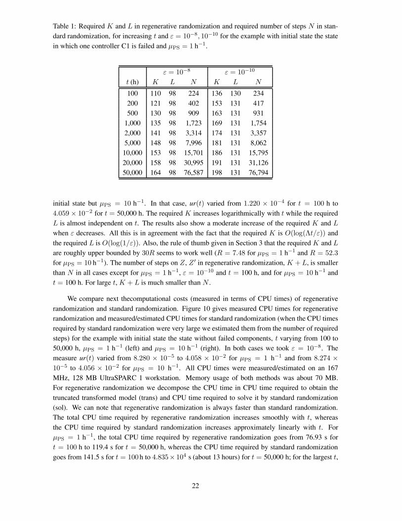
Table 1: Required K and L in regenerative randomization and required number of steps N in stan-dard randomization, for increasing t and ε = 10−8, 10−10 for the example with initial state the statein which one controller C1 is failed and μPS = 1 h−1.

ε = 10−8 ε = 10−10

t (h) K L N K L N

100 110 98 224 136 130 234200 121 98 402 153 131 417500 130 98 909 163 131 931

1,000 135 98 1,723 169 131 1,7542,000 141 98 3,314 174 131 3,3575,000 148 98 7,996 181 131 8,062

10,000 153 98 15,701 186 131 15,79520,000 158 98 30,995 191 131 31,12650,000 164 98 76,587 198 131 76,794

initial state but μPS = 10 h−1. In that case, ur(t) varied from 1.220 × 10−4 for t = 100 h to4.059 × 10−2 for t = 50,000 h. The required K increases logarithmically with t while the requiredL is almost independent on t. The results also show a moderate increase of the required K and Lwhen ε decreases. All this is in agreement with the fact that the required K is O(log(Λt/ε)) andthe required L is O(log(1/ε)). Also, the rule of thumb given in Section 3 that the required K and Lare roughly upper bounded by 30R seems to work well (R = 7.48 for μPS = 1 h−1 and R = 52.3for μPS = 10 h−1). The number of steps on Z , Z ′ in regenerative randomization, K +L, is smallerthan N in all cases except for μPS = 1 h−1, ε = 10−10 and t = 100 h, and for μPS = 10 h−1 andt = 100 h. For large t, K + L is much smaller than N .

We compare next thecomputational costs (measured in terms of CPU times) of regenerativerandomization and standard randomization. Figure 10 gives measured CPU times for regenerativerandomization and measured/estimated CPU times for standard randomization (when the CPU timesrequired by standard randomization were very large we estimated them from the number of requiredsteps) for the example with initial state the state without failed components, t varying from 100 to50,000 h, μPS = 1 h−1 (left) and μPS = 10 h−1 (right). In both cases we took ε = 10−8. Themeasure ur(t) varied from 8.280 × 10−5 to 4.058 × 10−2 for μPS = 1 h−1 and from 8.274 ×10−5 to 4.056 × 10−2 for μPS = 10 h−1. All CPU times were measured/estimated on an 167MHz, 128 MB UltraSPARC 1 workstation. Memory usage of both methods was about 70 MB.For regenerative randomization we decompose the CPU time in CPU time required to obtain thetruncated transformed model (trans) and CPU time required to solve it by standard randomization(sol). We can note that regenerative randomization is always faster than standard randomization.The total CPU time required by regenerative randomization increases smoothly with t, whereasthe CPU time required by standard randomization increases approximately linearly with t. ForμPS = 1 h−1, the total CPU time required by regenerative randomization goes from 76.93 s fort = 100 h to 119.4 s for t = 50,000 h, whereas the CPU time required by standard randomizationgoes from 141.5 s for t = 100 h to 4.835× 104 s (about 13 hours) for t = 50,000 h; for the largest t,

22

Table 2: Required K and L in regenerative randomization and required number of steps N in stan-dard randomization, for increasing t and ε = 10−8, 10−10 for the example with initial state the statein which one controller C1 is failed and μPS = 10 h−1.

ε = 10−8 ε = 10−10

t (h) K L N K L N

100 801 722 1,237 980 967 1,263200 886 722 2,362 1,120 967 2,398500 953 722 5,662 1,197 967 5,718

1,000 995 722 11,081 1,241 967 11,1592,000 1,035 722 21,820 1,282 967 21,9305,000 1,086 722 53,795 1,333 967 53,96910,000 1,124 722 106,833 1,371 967 107,07720,000 1,161 722 212,595 1,409 967 212,94050,000 1,210 722 529,116 1,458 967 529,660

regenerative randomization is 405 times faster than standard randomization. For μPS = 10 h−1, thetotal CPU time required by regenerative randomization goes from 545.4 s for t = 100 h to 1,035 sfor t = 50,000 h, whereas the CPU time required by standard randomization goes from 777.1 sfor t = 100 h to 3.363 × 105 s (about 4 days) for t = 50,000 h; for the largest t, regenerativerandomization is 325 times faster than standard randomization. Also interesting is the distributionof the CPU time required by regenerative randomization. For μPS = 1 h−1, the time spent solvingthe truncated transformed model by standard randomization is negligible compared to the time spentobtaining that model. However, for μPS = 10h−1, that time is significant for large t. This is because,being the maximum output rate of the truncated transformed model, equal to (1 + θ)maxi∈S λi,larger for μPS = 10 h−1, standard randomization becomes a relatively less efficient method to solvethe truncated transformed model. Figure 11 compares the CPU times of regenerative randomizationand standard randomization for the example with initial state the state with one controller C1 failedand ε = 10−8 for μPS = 1 h−1 (left) and μPS = 10 h−1 (right). In those cases, there is a crosspointtime t below which standard randomization is faster than standard randomization. For μPS = 1h−1,the CPU time required by regenerative randomization goes from 148.4 s for t = 100 h to 192.3 sfor t = 50,000 h, whereas the CPU time required by standard randomization goes from 140.9 sfor t = 100 h to 4.765 × 104 s for t = 50,000 h, making regenerative randomization 248 timesfaster than standard randomization for the largest t. For μPS = 10 h−1, the CPU time required byregenerative randomization goes from 1,088 s for t = 100 h to 1,585 s for t = 50,000 h, whereasthe CPU time required by standard randomization goes from 775.6 s for t = 100 h to 3.292 × 105 sfor t = 50,000, making regenerative randomization 208 times faster than standard randomizationfor the largest t.

Table 3 compares the K required by the regenerative randomization method and the K , K ′,which would be required were the error associated with the truncation of the transformed modelcontrolled by computing me

K(t) exactly, for the example with initial state the state without failedcomponents, ε = 10−8, and μPS = 1 h−1, 10 h−1. We can note that K is very close to K ′ (in most

23

10

100

1000

10000

1e5

1e6

100 1000 10000t (h)

RR (trans)RR (sol)

RR (total)SR

10

100

1000

10000

1e5

1e6

100 1000 10000t (h)

RR (trans)RR (sol)

RR (total)SR

Figure 10: CPU times in seconds required by regenerative randomization (RR) and standard ran-domization (SR) to solve the example with initial state the state without failed components andε = 10−8 for μPS = 1 h−1 (left) and μPS = 10 h−1 (right).

10

100

1000

10000

1e5

1e6

100 1000 10000t (h)

RR (trans)RR (sol)

RR (total)SR

10

100

1000

10000

1e5

1e6

100 1000 10000t (h)

RR (trans)RR (sol)

RR (total)SR

Figure 11: CPU times in seconds required by regenerative randomization (RR) and standard ran-domization (SR) to solve the example with initial state the state with one controller C1 failed andε = 10−8 for μPS = 1 h−1 (left) and μPS = 10 h−1 (right).

24

Table 3: Required K and K ′ for increasing t and ε = 10−8 for the example with initial state thestate without failed components and μPS = 1 h−1, 10 h−1.

μPS = 1 h−1 μPS = 10 h−1

t (h) K K ′ K K ′

100 106 106 770 770200 116 116 850 850500 125 125 916 916

1,000 130 130 959 9582,000 136 136 998 9985,000 143 143 1,049 1,048

10,000 148 148 1,086 1,08620,000 153 153 1,124 1,12350,000 159 159 1,173 1,172

cases equal and in some cases greater by one). Thus, the upper bounds for me′′K,L(t) and me

K(t)given in Section 2 seem to be, for class C models, quite tight.

5 Related work

Reference [5], which is based on [6], describes preliminary related work. In [5], it is consideredthe particular case in which A = 1 and all states in S are transient, the error associated with thetruncation of the transformed model is controlled by computing me′′

K,L(t), meK(t) using a numerical

Laplace inversion algorithm, and the approximated model solution maK,L(t), ma

K(t) is computedusing also a numerical Laplace inversion algorithm. That strategy for controlling the error associatedwith the truncation of the transformed model is expensive when the required K is large. Also,computing ma

K,L(t), maK(t) using a numerical Laplace inversion algorithm results in a method in

which the computation error is less well-controlled. Finally, [5] does not analyze the performanceof the method for class C models with the selection r = o.

6 Conclusions

We have developed a new method called regenerative randomization for the transient analysis of con-tinuous time Markov chain models with absorbing states. The method has the same good properties(numerical stability, well-controlled computation error, and ability to specify the computation errorin advance) as the well-known standard randomization method and can be significantly less costlythan that method for large models and large t. The method requires the selection of a regenerativestate, on which the performance of the method depends. Automatic selection of the regenerativestate seems to be difficult, in general, and the method relies on the user’s intuition to select a goodregenerative state. However, a class of models, class C, including typical failure/repair models with

25

exponential failure and repair time distributions and repair in every state with failed components, hasbeen identified for which a natural selection for the regenerative state exists and, for those models,theoretical results assessing approximately the performance of the method with that natural selectionin terms of “visible” model characteristics have been obtained. Those theoretical results can be usedto anticipate, for class C models and that natural selection for the regenerative state, when regen-erative randomization can be expected to be significantly less costly than standard randomization.Using an example belonging to that class, we have illustrated the performance of regenerative ran-domiztion and have shown that it can indeed be much faster than standard randomization, allowinga numerically stable transient analysis, with well-controlled and specifiable-in-advance computationerror, of very large CTMC models with absorbing states in affordable CPU times.

Acknowledgments

This work was supported by the “Comision Interministerial de Ciencia y Tecnologıa” (CICYT) ofthe Ministry of Science and Technology of Spain under the research grants TIC95-0707-C02-02 andTAP1999-0443-C05-05.

Appendix

Lemma 1. Let X and Y be finite CTMCs with identical state spaces and initial probability distri-

butions and transition rate matrices A and B, respectively. Let pX(t) and pY (t) be the probabilitydistribution column vectors of, respectively, X and Y at time t. Then

||pY (t) − pX(t)||1 ≤ ||BT −AT ||1t.

Proof. Vector pY (t) is the solution of

dpY

dt= BTpY (t),

which can be rewritten as

dpY

dt= ATpY (t) + (BT − AT )pY (t),

from which, since pX(t) = eAT tpX(0) and pX(0) = pY (0),

pY (t) = eAT tpY (0) +

∫ t

0eA

T (t−s)(BT − AT )pY (s) ds

= pX(t) +∫ t

0eA

T (t−s)(BT − AT )pY (s) ds,

which implies

||pY (t) − pX(t)||1 =∣∣∣∣∣∣∣∣∫ t

0eA

T (t−s)(BT − AT )pY (s) ds∣∣∣∣∣∣∣∣

1

≤∫ t

0||eAT (t−s)||1 ||BT − AT ||1 ||pY (s)||1 ds.

26

But ||pY (s)||1 = 1 and ||eAT (t−s)||1 = 1, since column i of eAT (t−s) is the probability distribution

vector of X at time t− s conditioned to X(0) = i, and the result follows.

Proof of Proposition 1 The initial probability distribution of V follows immediately from its def-inition (13). It is also clear that: 1) Vk ∈ {s0, s1, . . . , sk, s

′k, f1, f2, . . . , fA}, 2) from a state sl, V

can only jump to states fi, 1 ≤ i ≤ A, s0 and sl+1, and 3) from a state s′k, V can only jump tostates fi, 1 ≤ i ≤ A, s0 and s′k+1. Since Vk = fi if and only if Xk = fi and fi is absorbingin X , from state fi, V can only jump to fi and P [Vk+1 = fi | Vk = fi] = P [Vk+1 = fi | Vk =fi ∧ Vk−1 = xk−1 ∧ · · · ∧ V0 = x0] = 1. To completely verify that V is a DTMC we have to showthat P [Vk+1 = y | Vk = sl ∧ Vk−1 = xk−1 ∧ · · · ∧ V0 = x0] = P [Vk+1 = y | Vk = sl] for all feasiblepaths (x0, x1, . . . , xk−1, sl) of V and that P [Vk+1 = y | Vk = s′k ∧ Vk−1 = xk−1 ∧ · · · ∧ V0 =x0] = P [Vk+1 = y | Vk = s′k] for all feasible paths (x0, x1, . . . , xk−1, s

′k) of V . But, Vk = sl

implies Vk−l = s0, Vk−l+1 = s1, . . . , Vk−1 = sl−1 and, given the definition of V (13), the be-havior of V after the steps m at which V hits state s0 is independent of X0, X1, . . . , Xm−1 and,therefore, of V0, V1, . . . , Vm−1, and, then, P [Vk+1 = y | Vk = sl ∧ Vk−1 = sl−1 ∧ · · · ∧ Vk−l =s0 ∧ Vk−l−1 = xk−l−1 ∧ · · · ∧ V0 = x0] = P [Vk+1 = y | Vk = sl ∧ Vk−1 = sl−1 ∧ · · · ∧ Vk−l =s0] = P [Vk+1 = y | Vk = sl]. Similarly, Vk = s′k implies V0 = s′0, V1 = s′1, . . . , Vk−1 = s′k−1

and P [Vk+1 = y | Vk = s′k ∧ Vk−1 = s′k−1 ∧ · · · ∧ V0 = s′0] = P [Vk+1 = s′k+1 | Vk = s′k].It remains to verify the values of the transition probabilities from states s′l and sl. We will useVk ∈ {s0, s1, . . . , sk, s

′k, f1, f2, . . . , fA}.

Case a (P [Vk = s0] > 0, which implies (13) P [Xk = r] > 0): Taking into account the definition ofV (13), that πr(0) = 1 and πi(0) = 0, i ∈ S′, and the definition of a(l):

P [Vk+1 = fj | Vk = s0] =P [Vk = s0 ∧ Vk+1 = fj]

P [Vk = s0]=P [Xk = r ∧ Xk+1 = fj]

P [Xk = r]

= P [Xk+1 = fj | Xk = r] = Pr,fj=

∑i∈S πi(0)Pi,fj∑

i∈S πi(0)=

∑i∈S πi(0)Pi,fj

a(0)= vj

0.

Similarly, we have:

P [Vk+1 = s0 | Vk = s0] =P [Vk = s0 ∧ Vk+1 = s0]

P [Vk = s0]=P [Xk = r ∧ Xk+1 = r]

P [Xk = r]

= P [Xk+1 = r | Xk = r] = Pr,r =∑

i∈S πi(0)Pi,r∑i∈S πi(0)

=∑

i∈S πi(0)Pi,r

a(0)= q0,

P [Vk+1 = s1 | Vk = s0] =P [Vk = s0 ∧ Vk+1 = s1]

P [Vk = s0]=P [Xk = r ∧ Xk+1 ∈ S′]

P [Xk = r]

= P [Xk+1 ∈ S′ | Xk = r] = Pr,S′ =∑

i∈S πi(0)Pi,S′∑i∈S πi(0)

=∑

i∈S πi(0)Pi,S′

a(0)= w0.

Case b (P [Vk = sl] > 0, 1 ≤ l ≤ k, which implies P [Xk−l = r] > 0 (13)): Taking intoaccount the definition of V (13), that the DTMC {Xm+k; k = 0, 1, 2, . . .} conditioned to Xm = r

is probabilistically identical to X ′ = {X ′k; k = 0, 1, 2, . . .}, the definition of Z (3), that Zl �= r for

l ≥ 1 and, therefore, for l ≥ 1, Zl ∈ S′ if and only if Zl ∈ S, that (4) P [Zl+1 = fj |Zl = i] = Pi,fj,

i ∈ S, and the definition of a(l):

P [Vk+1 = fj | Vk = sl] =P [Vk = sl ∧ Vk+1 = fj]

P [Vk = sl]

27

=P [Xk−l = r ∧ Xk−l+1:k ∈ S′ ∧ Xk+1 = fj]

P [Xk−l = r ∧ Xk−l+1:k ∈ S′]

=P [Xk−l+1:k ∈ S′ ∧ Xk+1 = fj | Xk−l = r]

P [Xk−l+1:k ∈ S′ | Xk−l = r]

=P [X ′

1:l ∈ S′ ∧ X ′l+1 = fj]

P [X ′1:l ∈ S′]

=P [Zl ∈ S′ ∧ Zl+1 = fj]

P [Zl ∈ S′]=P [Zl ∈ S ∧ Zl+1 = fj]

P [Zl ∈ S]

=∑

i∈S πi(l)Pi,fj∑i∈S πi(l)

=∑

i∈S πi(l)Pi,fj

a(l)= vj

l .

Similarly, we have

P [Vk+1 = s0 | Vk = sl] =P [Vk = sl ∧ Vk+1 = s0]

P [Vk = sl]

=P [Xk−l = r ∧ Xk−l+1:k ∈ S′ ∧ Xk+1 = r]

P [Xk−l = r ∧ Xk−l+1:k ∈ S′]=P [Xk−l+1:k ∈ S′ ∧ Xk+1 = r | Xk−l = r]

P [Xk−l+1:k ∈ S′ | Xk−l = r]

=P [X ′

1:l ∈ S′ ∧ X ′l+1 = r]

P [X ′1:l ∈ S′]

=P [Zl ∈ S′ ∧ Zl+1 = a]

P [Zl ∈ S′]=P [Zl ∈ S ∧ Zl+1 = a]

P [Zl ∈ S]

=∑

i∈S πi(l)Pi,r∑i∈S πi(l)

=∑

i∈S πi(l)Pi,r

a(l)= ql,

P [Vk+1 = sl+1 | Vk = sl] =P [Vk = sl ∧ Vk+1 = sl+1]

P [Vk = sl]

=P [Xk−l = r ∧ Xk−l+1:k+1 ∈ S′]P [Xk−l = r ∧ Xk−l+1:k ∈ S′]

=P [Xk−l+1:k+1 ∈ S′ | Xk−l = r]

P [Xk−l+1:k ∈ S′ | Xk−l = r]

=P [X ′

1:l+1 ∈ S′]

P [X ′1:l ∈ S′]

=P [Zl+1 ∈ S′]P [Zl ∈ S′]

=P [Zl ∈ S ∧ Zl+1 ∈ S′]

P [Zl ∈ S]

=∑

i∈S πi(l)Pi,S′∑i∈S πi(l)

=∑

i∈S πi(l)Pi,S′

a(l)= wl.

Case c (P [Vk = s′k] > 0): Taking into account the definition of V (13), the definition of Z ′ (7), that(8) P [Z ′

k+1 = fj | Z ′k = i] = Pi,fj

, i ∈ S′, and the definition of a′(k):

P [Vk+1 = fj | Vk = s′k] =P [Vk = s′k ∧ Vk+1 = fj]

P [Vk = s′k]=P [X0:k ∈ S′ ∧ Xk+1 = fj ]

P [X0:k ∈ S′]

=P [Z ′

k ∈ S′ ∧ Z ′k+1 = fj]

P [Z ′k ∈ S′]

=

∑i∈S′ π′i(k)Pi,fj∑

i∈S′ π′i(k)=

∑i∈S′ π′i(k)Pi,fj

a′(k)= v′jk .

Similarly, we have:

P [Vk+1 = s0 | Vk = s′k] =P [Vk = s′k ∧ Vk+1 = s0]

P [Vk = s′k]=P [X0:k ∈ S′ ∧ Xk+1 = r]

P [X0:k ∈ S′]

=P [Z ′

k ∈ S′ ∧ Z ′k+1 = a]

P [Z ′k ∈ S′]

=∑

i∈S′ π′i(k)Pi,r∑i∈S′ π′i(k)

=∑

i∈S′ π′i(k)Pi,r

a′(k)= q′k,

28

P [Vk+1 = s′k+1 | Vk = s′k] =P [Vk = s′k ∧ Vk+1 = s′k+1]

P [Vk = s′k]=P [X0:k+1 ∈ S′]P [X0:k ∈ S′]

=P [Z ′

k+1 ∈ S′]P [Z ′

k ∈ S′]=P [Z ′

k ∈ S′ ∧ Z ′k+1 ∈ S′]

P [Z ′k ∈ S′]

=∑

i∈S′ π′i(k)Pi,S′∑i∈S′ π′i(k)

=∑

i∈S′ π′i(k)Pi,S′

a′(k)= w′

k.

Proof of Proposition 3 We start by considering the case αS′ > 0. Assuming P [(VK,L)0 = s0] > 0,let μ(k) = P [(VK,L)k = a | (VK,L)0 = s0]. We start by showing that μ(k) ≤ Ik>K(k −K)a(K).To that end define

ν(k) = P [(VK,L)k = s0 ∧ (VK,L)1:k−1 �= s0 | (VK,L)0 = s0], k ≥ 1.

In words, ν(k) is the probability that, starting at s0, VK,L hits for first time s0 after k steps. Notethat, from the state transition diagram of VK,L (Figure 4), ν(k) = 0 for k > K. For 1 ≤ k ≤ K

using (17), Proposition 1, and a(k) = a(k − 1) − ∑i∈S πi(k − 1)(Pi,r +

∑Aj=1 Pi,fj

),

ν(k) =

(k−2∏i=0

wi

)qk−1 = a(k − 1)

∑i∈S πi(k − 1)Pi,r

a(k − 1)

= a(k − 1)a(k − 1) − a(k) − ∑

i∈S πi(k − 1)∑A

j=1 Pi,fj

a(k − 1)

≤ a(k − 1)a(k − 1) − a(k)

a(k − 1)= a(k − 1) − a(k). (22)

Since at least K + 1 steps are required for VK,L to arrive to a from s0, μ(k) = 0 for k ≤ K. Fork ≥ K + 1, the result μ(k) ≤ (k −K)a(K) is shown by complete induction on k. The base case isk = K + 1. For k = K + 1 the only path from s0 to a with K + 1 steps is (s0, s1, . . . , sK , a) and(17)

μ(K + 1) =K−1∏i=0

wi = a(K).

Let us proceed with the induction step. Assume μ(l) ≤ (l −K)a(K) for K + 1 ≤ l < k and let usprove the result for k > K+1. Let i′max = min{K,k−K−1}. Classifying the paths of VK,L withk steps which start at s0 and end in a into those which do so without revisiting s0 and those whichdo so by re-entering s0 for first time after i steps, 1 ≤ i ≤ i′max, using (17), (22), the inductionhypothesis, and a(0) = 1, noting that i′max ≥ 1 (because K ≥ 1 and k > K + 1), we have

μ(k) =K−1∏i=0

wi +i′max∑i=1

ν(i)μ(k − i) = a(K) +i′max∑i=1

ν(i)μ(k − i)

≤ a(K) +i′max∑i=1

(a(i− 1) − a(i)

)(k − i−K)a(K)

=

⎡⎣1 +i′max∑i=1

(a(i− 1) − a(i)

)(k −K − i)

⎤⎦ a(K)

=

⎡⎣1 + a(0)(k −K − 1) −i′max−1∑

i=1

a(i) − a(i′max)(k −K − i′max)

⎤⎦ a(K)

29

< [1 + k −K − 1]a(K) = (k −K)a(K),

completing the induction step.

Letψ(k) = P [(VK,L)k = s0 ∧ (VK,L)1:k−1 �= s0 | (VK,L)0 = s′0], k ≥ 1.

In words, ψ(k) is the probability that, starting at s′0, VK,L hits s0 for first time after k steps. Fromthe state transition diagram of VK,L (Figure 4), it is clear that ψ(k) = 0 for k > L. For 1 ≤ k ≤ L,using (18), Proposition 1, and a′(k) = a′(k − 1) − ∑

i∈S′ π′i(k − 1)(Pi,r +∑A

j=1 Pi,fj):

ψ(k) =

(k−2∏i=0

w′i

)q′k−1 =

a′(k − 1)αS′

∑i∈S′ π′i(k − 1)Pi,r

a′(k − 1)

=a′(k − 1)αS′

a′(k − 1) − a′(k) − ∑i∈S′ π′i(k − 1)

∑Aj=1 Pi,fj

a′(k − 1)

≤ a′(k − 1)αS′

a′(k − 1) − a′(k)a′(k − 1)

=a′(k − 1) − a′(k)

αS′. (23)

Let i′′max = min{L, k − K − 1}. Classifying the paths of VK,L which hit a through sK intothose which do so starting at s′0 and hitting s0 for first time after i steps, 1 ≤ i ≤ i′′max, and thosewhich start at s0, and using μ(k) ≤ Ik>K(k −K)a(K) and (23):

cK,L(k) = αS′

i′′max∑i=1

ψ(i)μ(k − i) + αrμ(k)

≤i′′max∑i=1

(a′(i− 1) − a′(i)

)(k − i−K)a(K) + αrIk>K(k −K)a(K). (24)

For k ≤ K + 1, i′′max ≤ 0 and∑i′′max

i=1 (a′(i − 1) − a′(i))(k − i −K)a(K) = 0. For k > K + 1,since L ≥ 1, i′′max ≥ 1 and, noting that a′(0) = αS′ ,

i′′max∑i=1

(a′(i− 1) − a′(i)

)(k − i−K)a(K)

=

⎡⎣a′(0)(k −K − 1) −i′′max−1∑

i=1

a′(i) − a′(i′′max)(k −K − i′′max)

⎤⎦ a(K)

< αS′(k −K − 1)a(K).

In summary, we have

i′′max∑i=1

(a′(i− 1) − a′(i)

)(k − i−K)a(K) ≤ Ik>K+1αS′(k −K − 1)a(K).

Finally, substituting in (24),

cK,L(k) ≤ Ik>K+1αS′(k −K − 1)a(K) + Ik>Kαr(k −K)a(K)

≤ Ik>KαS′(k −K)a(K) + Ik>Kαr(k −K)a(K) = Ik>KαS(k −K)a(K).

30

It remains to deal with the particular case αS′ = 0. In that case, cK(k) = αSμ(k) and, as it hasbeen shown, μ(k) ≤ Ik>K(k −K)a(K).

Proof of Theorem 3 We start by upper bounding the terms in the upper bounds for the error asso-ciated with the truncation of the transformed model used in regenerative randomization. Trivially,

rmaxa′(L)

∞∑k=L+1

e−Λt (Λt)k

k!< rmaxa

′(L). (25)

Also,

rmaxαSa(K)∞∑

k=K+1

(k −K)e−Λt (Λt)k

k!= rmaxαSa(K)

∞∑k=1

ke−Λt (Λt)K+k

(K + k)!

< rmaxαSa(K)∞∑

k=1

e−Λt (Λt)K+k

(K + k − 1)!= rmaxαSa(K)Λt

∞∑k=1

e−Λt (Λt)K+k−1

(K + k − 1)!

= rmaxαSa(K)Λt∞∑

k=K

e−Λt (Λt)k

k!< rmaxαSa(K)Λt. (26)

Being all states i ∈ S of Z transient, πi(k), i ∈ S decrease geometrically fast [31, Theorem4.3] and, since a(k) =

∑i∈S πi(k), so does a(k). This implies that there exist k0 ≥ 0, B > 0 and

b, 0 < b < 1 such thata(k) ≤ Bbk, k ≥ k0. (27)

Similarly, for αS′ > 0, using the fact that all states i ∈ S′ of Z ′ are transient, there exists k′0 ≥ 0,B′ > 0, and b′, 0 < b′ < 1 such that

a′(k) ≤ B′b′k, k ≥ k′0. (28)

We start by considering the case αS′ > 0. Using (26), the required K is upper bounded bythe minimum integer k ≥ 1 satisfying rmaxαSa(k)Λt ≤ ε/4. Using (27), that integer is not greaterthat max{k0, l}, where l is the minimum integer ≥ 1 satisfying rmaxαSBb

lΛt ≤ ε/4. Then, toprove that K is O(log(Λt/ε)), it suffices to prove that l is O(log(Λt/ε)). But l is not greater thanmax{1, �x� + 1}, where x satisfies

rmaxαSBbxΛt =

ε

4.

Taking logarithms:

log rmax + log αS + logB + x log b+ log(Λt) = log(ε

4

),

x =log(4Λt/ε) + log rmax + logαS + logB

log(1/b).

Being 0 < b < 1, log(1/b) > 0, showing that x, l and K are O(log(Λt/ε)).

For the case αS′ > 0, using (25), the required L is upper bounded by the minimum integerk ≥ 1 satisfying rmaxa

′(k) ≤ ε/4. Using (28), that integer is not greater than max{k′0, l}, where

31

l is the minimum integer ≥ 1 satisfying rmaxB′b′l ≤ ε/4. Then, to prove that L is O(log(1/ε)), it

suffices to prove that l is O(log(1/ε)). But l is not greater than max{1, �x� + 1}, where x satisfies

rmaxB′b′x =

ε

4.

Taking logarithms:log rmax + logB′ + x log b′ = log

(ε4

),

x =log(4/ε) + log rmax + logB′

log(1/b′),

and, being 0 < b′ < 1, log(1/b′) > 0, showing that x, l and L are O(log(1/ε)).

The proof that, for the case αS′ = 0, the required K is O(log(Λt/ε)) follows the proof that,for the case αS′ > 0, the required K is O(log(Λt/ε)) with ε replaced by 2ε (because the allocatedmodel truncation error is ε/2 instead of ε/4).

References

[1] M. Abramowitz and I. A. Stegun, eds., Handbook of Mathematical Functions, Dover, 1964.

[2] C. Beounes, M. Aguera, J. Arlat, S. Bachman, C. Bourdeu, J. E. Doucet, K. Kanoun, J. C. Laprie,S. Metge, J. Moreira de Souza, D. Powell and P. Spiesser, “SURF-2: A Program for DependabilityEvaluation of Complex Hardware and Software Systems,” in Proc. 23rd IEEE Int. Symp. on Fault-Tolerant Computing (FTCS-23), Toulouse, June 1993, pp. 142–150.

[3] A. Bobbio and M. Telek, “A Benchmark for PH Estimation Algorithms: Results for Acyclic-PH,” Com-munications in Statistics—Stochastic Models, vol. 10, no. 3, 1994, pp. 661–677.

[4] P. N. Bowerman, R. G. Nolty and E. M. Schener, “Calculation of the Poisson Cumulative DistributionFunction,” IEEE Trans. on Reliability, vol. 39, no. 2, 1990, pp. 158–161.

[5] A. Calderon and J. A. Carrasco, “Computation of Absorption Probability Distributions of continuous-time Markov chains using Regenerative Randomization,” in Proc. IEEE Int. Computer Performanceand Dependability Symposium, 1995, Erlangen, April 1995, pp. 92–101.

[6] J. A. Carrasco and A. Calderon, “Regenerative Randomization: Theory and application examples,”Performance Evaluation Review, vol. 23, no. 1, May 1995, pp. 241–252.

[7] G. Ciardo, J. Muppala and K. Trivedi, “SPNP: Stochastic Petri Net Package,” in Proc. 3rd IEEE Int.Workshop on Petri Nets and Performance Models, PNPM89, Kyoto, December 1989, pp. 142–151.

[8] J. Couvillon, R. Freire, R. Johnson, W. Obal II, A. Qureshi, M. Rai, W. Sanders and J. Tvedt, “Per-formability modelling with UltraSAN,” IEEE Software, September 1991, pp. 69–80.

[9] B. L. Fox and P. W. Glynn, “Computing Poisson probabilities,” Communications of the ACM, vol. 31,1988, pp. 440–445.

[10] A. Goyal, W. C. Carter, E. de Souza e Silva and S. S. Lavenberg, “The System Availability Estimator,”in Proc. 16th IEEE Int. Symp. on Fault-Tolerant Computing (FTCS-16), July 1986, pp. 84–89.

[11] W. K. Grassman, “Transient solutions in Markovian queuing systems,” Computers and Operations Re-search, vol. 4, 1977, pp. 47–53.

32

[12] W. K. Grassman, “Rounding Errors in Certain Algorithms Involving Markov Chains,” ACM Transac-tions on Mathematical Software, vol. 19, no. 4, December 1993, pp. 496–508.

[13] D. Gross and D. R. Miller, “The randomization technique as a modelling tool and solution procedurefor transient Markov processes,” Operations Research, vol. 32, 1984, pp. 343–361.

[14] B. W. Johnson, Design and Analysis of Fault Tolerant Digital Systems, Addison-Wesley, 1989.

[15] M. Kijima, Markov Processes for Stochastic Modeling, University Press, Cambridge, 1997.

[16] L. Knusel, “Computation of the Chi-square and Poisson Distribution,” SIAM J. Sci. Stat. Comput., vol. 7,no. 3, July 1986, pp. 1022–1036.

[17] M. Malhotra, J. K. Muppala and K. S. Trivedi, “Stiffness-Tolerant Methods for Transient Analysis ofStiff Markov Chains,” Microelectronics and Reliability, vol. 34, no. 11, 1994, pp. 1825–1841.

[18] M. Malhotra, “A computationally efficient technique for transient analysis of repairable Markoviansystems,” Performance Evaluation, November 1995, no. 1–2, pp. 311–331.

[19] B. Melamed and M. Yadin, “Randomization Procedures in the Computation of Cumulative-Time Dis-tributions over Discrete State Markov Processes,” Operations Research, vol. 32, 1984, pp. 926–944.

[20] D. R. Miller, “Reliability Calculation using Randomization for Markovian Fault-Tolerant ComputingSystems,” in Proc. 13th IEEE Int. Symp. on Fault-Tolerant Computing (FTCS-13), June 1983, pp 284–289.

[21] A. P. Moorsel and W. H. Sanders, “Adaptive Uniformization”, Communications in Statistics–StochasticModels, vol. 10, no. 3, 1994, pp. 619–647.

[22] A. P. Moorsel and W. H. Sanders, “Transient Solution of Markov Models by Combining Adaptive andStandard Uniformization,” IEEE Trans. on Reliability, vol. 46, no. 3, 1997, pp. 430–440.

[23] H. Nabli and B. Sericola, “Performability Analysis: A New Algorithm,” IEEE Trans. on Computers,vol. 45, no. 4, April 1996, pp. 491–494.

[24] F. Neuts, Matrix-Geometric Solutions in Stochastic Models. An Algorithmic Approach, Dover Publica-tions Inc., New York, 1994.

[25] M. A. Qureshi and W. H. Sanders, “Reward Model Solution Methods with Impulse and Rate Rewards:An Algorithm and Numerical Results,” Performance Evaluation, vol. 20, 1994, pp. 413–436.

[26] A. Reibman and K. S. Trivedi, “Numerical Transient Analysis of Markov Models,” Computers andOperations Research, vol. 15, 1988, pp. 19–36.

[27] S. M. Ross, Stochastic Processes, John Wiley & Sons, 1983.

[28] G. Rubino and B. Sericola, “Interval Availability Distribution Computation,” in Proc. 23th Int. Symp.on Fault-Tolerant Computing (FTCS-23), Toulouse, June 1993, pp. 48–55.

[29] G. Rubino and B. Sericola, “Interval Availability Analysis Using Denumerable Markov Processes: Ap-plication to Multiprocessor Subject to Breakdowns and Repair,” IEEE Trans. on Computers, vol. 44,no. 2, February 1995, pp. 286–291.

[30] J. R. Schott, Matrix Analysis for Statistics, John Wiley & Sons, Inc., 1997.

[31] E. Seneta, Non-negative Matrices and Markov Chains, Springer Series in Statistics, Springer-Verlag,2nd edition, 1981.

33

[32] B. Sericola, “Availability Analysis of Repairable Computer Systems and Stationarity Detection,” IEEETrans. on Computers, vol. 48, no. 11, November 1999, pp. 1166–1172.

[33] E. de Souza e Silva and H. R. Gail, “Calculating Cumulative Operational Time Distributions of Re-pairable Computer Systems,” IEEE Trans. on Computers, vol. 35, 1986, pp. 322–332.

[34] E. de Souza e Silva and H. R. Gail, “Calculating Availability and Performability Measures of RepairableComputer Systems using Randomization,” Journal of the ACM, vol. 34, 1989, pp. 179–199.

[35] E. de Souza e Silva and H. R. Gail, “An Algorithm to Calculate Transient Distributions of CumulativeRate and Impulse Based Reward,” Communications in Statistics–Stochastic Models, vol. 14, no. 3,1998, pp. 509–536.

[36] M. R. Spiegel, Mathematical Handbook of Formulas and Tables, McGraw-Hill, 1970.

[37] R. S. Varga, Matrix Iterative Analysis, Prentice-Hall, Inc., 1962.

34