Trajectory planning under a Stochastic Uncertainty

Ulf T. JonssonOptimization and Systems Theory

Royal Institute of TechnologySE-100 44 Stockholm, Sweden

Clyde MartinDepartment of Mathematics and Statistics

Texas Tech UniversityLubbock, Texas, USA

Yishao ZhouDepartment of Mathematics

Stockholm UniversitySE-106 91 Stockholm, Sweden

Abstract

A trajectory planning problem for linear stochastic differential equations is considered in thispaper. The aim is to control the system such that the expected value of the output interpolatesgiven points at given times while the variance and an integral cost of the control effort areminimized. The solution is obtained by using the dynamic programming technique, whichallows for several possible generalizations that are also considered. The results of this papercan be used for control of systems with a stochastic growth rate. This is frequently the case ininvestment problems and in biomathematics.

1 Introduction

We are concerned with controlling the state or some measured quantity of the state to given valuesat discrete times. That is given a system of the form

x = f(x) + u1g1(x) + · · · + ukgk(x)

andy = Cx

where x ∈ Rn and y ∈ R

p we look for a system of controls that drive the output through or closeto a prescribed sequence of set points

{y(ti) = αi : i = 1, · · · , N}.

In this paper we specialize this problem to one in which the system is linear but the evolutionequation is stochastic. Such systems occur in a variety of settings. We consider a rather completeexample of a model that contains variable interest rates in Section 3. A second example, consideredin Section 4, is trajectory planning for a feedback linearized mobile robot. Here the combined effectof surface irregularities, friction, and other disturbances is modeled as a multiplicative stochasticdisturbance. Another set of problems occurs in biomathematics when considering the chemostat.There are extensive references on physical, biological and mathematical background of the chemo-stat available in the literature, see for example [5]. In many situations the nutrient content of

1

the chemostat is not deterministic and a better model would be obtained by replacing the lineargrowth rate of the standard models by a random variable. This variable reflects the rate at whichthe nutrient is consumed and/or naturally degrades. This rate is a function of temperature andmany other variables that are not modelled and hence could and should be taken to be stochastic.It is beyond the scope of this paper to consider a complete analysis of such systems but a model inthis form fits the theory described in this paper.

The specific topic of this paper is the problem of designing a feedback control for a linear stochasticdifferential equation in such a way that the mean value of a specific output interpolates given pointsat given times at the same time as the variance and the expected value of an integral quadraticcost along the trajectory are minimized. By minimizing the variance at the interpolation points weminimize effect of uncertainty due to the diffusion term in the system equation. By using a newnotation we obtain compact formulas for the design equations. The problem is related to severalmethods based on optimal control for interpolating splines that recently have been proposed inthe literature, see for example [4, 3, 12]. Apart from considering stochastic models, this paperdistinguishes itself by using a dynamic programming approach which leads to feedback solutions ofthe corresponding control problem.

In Section 5 we discuss a generalization, where we optimize over a finite set of possible interpo-lation points at each time instance. This problem reminds of the standard shortest path problem,see e.g. [1], but is complicated by the dynamic nature which make the cost corresponding to eachnode dependent on future interpolation points as well as the initial condition. The complexity ofthis problem can be reduced by considering suboptimal techniques such as discretization or treepruning. We briefly review some related work in [2, 6, 8, 9].

2 Stochastic Trajectory Planning

We consider a path planning problem where a stochastic disturbance enters the differential equation.As our basic problem we consider

J0(x0) = minu∈M(t0,tN )

N−1∑

k=0

wk+1Var2{CX(tk+1)} + Et0,x0

{∫ tN

0|u|2dt

}

subject to

{dX = (AX + Bu)dt + G(X)dZ, X(t0) = x0

Et0,x0{CX(tk+1)} = αk+1, k = 0, . . . , N − 1

(2.1)

where wk ≥ 0 and (A, B) is a controllable pair. The last term in the stochastic differential equationcorresponds to a multiplicative noise on the state vector defined by a m-dimensional Brownianmotion Zt. In other words, Zt is a process with zero mean and independent increments, i.e.E{dZtdZ

Ts } = δ(t − s)Idt, where δ denotes the dirac function. We assume that G(x) is a linear

function on the form

G(x) =n∑

i=1

xiGi

where Gk ∈ Rn×m. In (2.1), Et0,x0 is the expectation operator given that X(t0) = x0 and

Var2{CX(tk)} = Et0,x0{(CX(tk) − Et0,x0{CX(tk)})2}.

2

We consider optimization over all Markov controls, i.e. feedback controls on the form u(t, ω) =µ(t, X(t, ω)). We let M(t0, tN ) denote the set of Markov controls on an interval (t0, tN ). It can beshown that our optimal solution also is optimal over all F t adapted processes, where Ft denotesthe σ algebra generated by Zs for s ≤ t, see e.g. [10].

It turns out that there will be linear and constant terms in the value function due to the varianceterm in the objective function. It is therefore no essential addition in complexity to consider amore general path planning problem, where we allow the dynamics to be time-varying and differentfrom stage to stage. We also consider integral costs that penalizes the state vector. This gives thefollowing generalization of (2.1).

J0(x0) = minu∈M(t0,tN )

Et0,x0

{N−1∑

k=0

(wk+1|C1X(tk+1) − βk+1|2 +

∫ tk+1

tk

σk(t, X, u)dt

)}

subject to

{dX = (Ak(t)X + Bk(t)u)dt + Gk(t, X)dZ, t ∈ [tk, tk+1], X(t0) = x0

Et0,x0{C2X(tk+1)} = αk+1, k = 0, . . . , N − 1

(2.2)

where

σk(t, x, u) = xT Qk(t)x + 2xT Sk(t)u + uT Rk(t)u + 2qk(t)T x + 2rk(t)T u + �k(t)

and

Gk(t, x) =n∑

i=1

xiGk,i(t)

and where everything else is defined in a similar way as in (2.1). Here Ak, Bk, Qk, . . . , ρk and Gk,i

are piecewise continuous functions of time and all pairs (Ak(t), Bk(t)) are assumed to be completelycontrollable and the cost is strictly convex, which is the case if for all t ∈ [tk, tk+1], k = 0, . . . , N−1,we have

Rk(t) > 0 and

[Qk(t) Sk(t)Sk(t)T Rk(t)

]≥ 0 (2.3)

Note that if C1 = C2 = C and αk = βk then Et0,x0{|CX(tk) − βk|2

}= Var2{CX(tk)}.

Let us define the cost-to-go functions

Jk(x) = minu∈M(tk,tN )

Etk,x

{N−1∑

i=k

(wi+1|C1X(ti+1) − βi+1|2 +

∫ ti+1

ti

σi(t, X, u)dt

)}

subject to

{dX = (Ai(t)X + Bi(t)u)dt + Gi(t, X)dZ, t ∈ [ti, ti+1], X(tk) = x

Et0,x0{C2X(ti+1)} = αi+1, i = k, . . . , N − 1

JN (x) =0(2.4)

Due to the Markov property of the stochastic differential equation we can use dynamic programmingto solve (2.1). We next state two propositions and then the main result that solves (2.1). The firststates the dynamic programming recursion.

3

Proposition 2.1. The optimal cost satisfies the following dynamic programming equation.

Jk(x) = minu∈M(tk,tk+1)

Etk,x

{∫ tk+1

tk

σk(t, X, u)dt + wk+1|C1X(tk+1) − βk+1|2 + Jk+1(X(tk+1))}

subject to

{dX = (Ak(t)X + Bk(t)u)dt + Gk(t, X)dZ, X(tk) = x

Etk,x{C2X(tk+1)} = αk+1

JN (x) = 0

The next proposition states the solution to the following stochastic optimal control problem. Itshows that Jk(x) is a quadratic function which is instrumental in solving the dynamic programmingiteration.

V (x0, α, t0, tf ) = minu∈M(t0,tf )

Et0,x0

{∫ tf

t0

σ(t, X(t), u(t))dt + X(tf )T Q0X(tf ) + 2qT0 X(tf ) + �0

}

subject to

{dX = (A(t)X + B(t)u)dt + G(t, X)dZ, X(t0) = x0

Et0,x0{CX(tf )} = α

(2.5)

where

σ(t, x, u) = xT Q(t)x + 2xT S(t)u + uT R(t)u + 2q(t)T x + 2r(t)T u + �(t)

and where Q, R, and S satisfies the conditions in (2.3).

Proposition 2.2. We have

V (x0, α, t0, tf ) = xT0 P (t0)x0 + 2p(t0)T x0 + ρ(t0) + (N(t0)T x0 + m(t0))T W (t0)−1(N(t0)T x0 + m(t0))

where

P + AT P + PA + Q + Π(P ) = (PB + S)R−1(PB + S)T , P (tf ) = Q0

N + (A − BR−1(BT P + ST ))T N = 0, N(tf ) = CT

p + (A − BR−1(BT P + ST ))T p + q = (PB + S)R−1r, p(tf ) = q0

W + NBR−1BT N = 0, W (tf ) = 0

m = NT BR−1(BT p + r), m(tf ) = −α

ρ + � = (r + BT p)T R−1(r + BT p), ρ(tf ) = �0

(2.6)

and where Π(P ) is a linear matrix function with elements Π(P )k,l = 12tr(GT

k PGl). The optimalcontrol is

u∗ = −R−1(BT P + ST )X − R−1BT Nv − R−1(BT p + r)

with v = −W (t0)−1(N(t0)T x0 + m(t0)).

Remark 2.1. If Q, R and S satisfies a condition analogous to (2.3), then the linearly perturbedRiccati equation in (2.6) has an absolutely continuous unique positive semidefinite solution [11].All other differential equations in (2.6) are linear with bounded piecewise continuous coefficients,which ensure existence of unique absolutely continuous solutions. Note also that we have W (t) > 0for t ∈ [t0, tf ) by the complete controllability of (A(t), B(t)).

4

Proof. The proof is done by Lagrangian relaxation of the linear constraint. See Appendix A forthe complete details.

In order to obtain a compact notation we introduce

Q0 =

[Q0 q0

qT0 �0

], Q =

[Q q

qT �

], S =

[S

rT

],

P =

[P p

pT ρ

], N =

[N

mT

], W = W, R = R

A =

[A 00 0

], B =

[B

0

], C(α) =

[C −α

],

G(t, x) =

[G(t, x)

0

], Π(P ) =

[Π(P ) 0

0 0

].

(2.7)

If we finally let X =[XT 1

]Tand x0 =

[xT

0 1]T

then the optimization problem (2.5) can bewritten

V (x0, α, t0, tf ) = minu∈M(t0,tf )

Et0,x0

{∫ tf

t0

[XT QX + 2XT Su + uT Ru]dt + X(tf )T Q0X(tf )}

subject to

{dX = (A(t)X + B(t)u)dt + G(t, X)dZ, X(t0) = x0

Et0,x0{C(α)X(tf )} = 0

(2.8)

and the optimal solution can be written

V (x0, α, t0, tf ) = xT0

[P (t0) + N(t0)W (t0)−1N(t0)T

]x0

where

˙P + AT P + P A + Q + Π(P ) = (P B + S)R−1(P B + S)T , P (tf ) = Q0

˙N + (A − BR−1(BT P + ST ))T N = 0, N(tf ) = C(α)T

˙W + NT BR−1BT N = 0, W (tf ) = 0

The optimal control is

u∗ = −R−1(BT P + S)x − R−1BT NW (t0)−1N(t0)T x0

There is an equivalent feedback form given as u∗ = −R−1(BT (P + NW−1NT ) + ST )X.We can now state the solution of the general stochastic trajectory planning problem in (2.2).

Proposition 2.3. Consider the optimal control problem in (2.2), where the condition (2.3) holds.The optimal Markov control in each time interval [tk, tk+1] is (all variables are defined analogouslywith (2.7))

u∗(t) = −Rk(t)−1(Bk(t)T Pk(t) + Sk(t)T )X(t) − Rk(t)−1Bk(t)T Nk(t)Wk(tk)−1Nk(tk)T X(tk)

5

where for k = N − 1, . . . , 0

˙P k + AT

k Pk + PkAk + Qk + Πk(Pk) = (PkBk + Sk)R−1k (PkBk + Sk)T ,

˙Nk + (Ak − BkR

−1k (BT

k Pk + STk ))T Nk = 0, Nk(tk+1) = C2(αk+1)T ,

˙W k + NT

k BkR−1k BT

k Nk = 0, Wk(tk+1) = 0,

and where PN−1(tN ) = wN C1(βN )T C1(βN ) and for k = N − 2, N − 3, . . . , 0

Pk(tk+1) = Pk+1(tk+1) + Nk+1(tk+1)Wk+1(tk+1)−1Nk+1(tk+1)T + wk+1C1(βk+1)T C1(βk+1).

The cost-to-go is

Jk(x) = xT[Pk(tk) + Nk(tk)Wk(tk)−1Nk(tk)T

]x.

Proof. By dynamic programming.

The formulation of Proposition 2.3 in the compact notation (2.7) gives appealing formulas butin a numerical implementation it is more efficient to perform computations using a system on theform (2.6). For the basic trajectory planning in (2.1) this reduces to the following result

Corollary 2.1. Consider the optimal control problem in (2.1), where the pair (A, B) is controllable.The optimal Markov control in each time interval [tk, tk+1] is

u∗(t) = −R−1BT Pk(t)X(t) − R−1BT Nk(t)vk − R−1BT pk(t)

with vk = −Wk(tk)−1(Nk(tk)T X(tk) + mk(tk)), where

Pk + AT Pk + PkA + Π(Pk) = PkBR−1BT Pk,

Nk + (A − BR−1BT Pk)T Nk = 0,

pk + (A − BR−1BT Pk)T pk = 0,

Wk + NTk BR−1BT Nk = 0,

mk = NTk BR−1BT pk,

ρk = pTk BR−1BT pk,

(2.9)

where Π(Pk) is a linear matrix function with elements Π(P )k,l = 12tr(GT

k PGl) and the boundaryconditions are

Pk(tk+1) = Pk+1(tk+1) + Nk+1(tk+1)Wk+1(tk+1)−1Nk+1(tk+1)T + wk+1CT C

pk(tk+1) = pk+1(tk+1) + Nk+1(tk+1)Wk+1(tk+1)−1mk+1(tk+1) + wk+1αTk+1C

T

ρk(tk+1) = ρk+1(tk+1) + mk+1(tk+1)T Wk+1(tk+1)−1mk+1(tk+1) + wk+1αTk+1αk+1

and Nk(tk+1) = CT , mk(tk+1) = −αk+1 and Wk(tk+1) = 0.The optimal cost-to-go is

Jk(x) = xT Pk(tk)x + 2pk(tk)T x + ρk(tk) + (Nk(tk)T x + mk(tk))T Wk(tk)−1(Nk(tk)T x + mk(tk))

6

3 A Homeowners Investment Problem

We consider a very simple problem arising in portfolio optimization. For most people their home isthe most dominant feature of the portfolio. In this example we consider the problem of controllingthe investment in the home when interest rates fluctuate and inflation, either positive or negative,occurs. In this example we are aware that in addition to making monthly payments the homeownerwill usually make improvements to the home thus increasing the value over and above the increasecaused by inflation, some features of the home deprecate lowering the value of the home and thehomeowner has the option to borrow against the value of the home at several points during thecourse of ownership. We model the value of the home in terms of two linear stochastic differentialequations and allow the noise to enter as a multiple of the state. The variables are categorized inTable 3.

P (t) is the principal remaining on the loan at time t

P0 initial purchase price

V (t) the actual market value of the home at time t

u1(t) the amount of cash either paid toward the principaland interest or withdrawn from the home in terms ofequity loans

u2(t) money applied to the value of the house in terms ofimprovements or taken form the value of the housethrough the sale of assets

dZ(t) a Brownian motion processes representing inflationand fluctuation in interest

i nominal annual interest rate

Table 1: Variables

We begin by considering the discrete time case. The fundamental law of payments can beexpressed as the principal at time n + 1 is equal to the principal at time n plus interest drawnduring the time period plus or minus the payment, i.e.,

Pn+1 = (1 + in)Pn ± Qn

where Pn denotes principal, in denotes the interest in the nth period and Qn denotes the nthpayment. Now using the notation from the table we have

P (t + h) = P (t) + h(i(t)P (t) − u1(t) + u2(t)), P (0) = P0 (3.10)

where u1(t) is rate of payment. The control u2(t) represents money borrowed from the bank tomake improvements. This variable enters into the equation for the value of the house. We divide

7

the interest rate into two parts. The first is a nominal rate and the second is ”random” motion ofthe rate. For the sake of simplicity we assume that this rate is equal to the rate of inflation. Wecan think of i(t) = i + Z(t + h)−Z(t) where Z(t + h)−Z(t) is an increment of Brownian motion.

The second part of the model is the market value of the home. Here we have

V (t + h) = V (t) + hu2(t) + (Z(t + h) − Z(t))V (t), V (0) = P0 (3.11)

We allow both u1 and u2 to be either positive or negative. If u1 is negative we consider this tobe money that is withdrawn from the value of the home as an equity loan. If u2 is negative weconsider this to be money that is achieved through the sale of assets associated with home. Anysuch money will be assumed to be applied to the principal. This is not a real restriction since wecan immediately borrow this money in terms of an equity loan. We can pass to the limit to obtaina continuous time model.

For the continuation of this model we take the following equations describing the evolution ofthe value of the home.

dP (t) = iP (t)dt + (u2(t) − u1(t))dt + P (t)dZ(t), P (0) = P0 (3.12)

dV (t) = V (t)dZ(t) + u2(t)dt, V (0) = P0 (3.13)

In the first equation we see that dZ(t) can denote the variation that occurs in interest rates.This is of course an approximation of reality. It is unlikely that interest rates would ever becomenegative and in most home loans there is a provision to bound from above the interest rate. Theincorporation of these bounds complicates the problem and obscures the application that we wishto exhibit. In the second equation dZ(t) denotes the effect of inflation on the value of the home.At one time it would not have seemed reasonable to have negative inflation. However during the1990s and into the beginning of the 21 century we have seen negative inflation in Japan. To usethe same rate for inflation and interest fluctuation is not entirely correct but for the purpose of anexample to support the theory developed in this paper it is adequate.

The variable of primary interest is a linear combination of P (t) and V (t). We let

Y (t) = V (t) − P (t) (3.14)

this variable represents the cash value of the home. A reasonable objective is to ask that Y (t)should double during the thirty years of the standard loan. That is we state as one objective that

E{Y (30)} = 2P0

where E{·} denotes expected value. In general we might expect that y(t) should follow a curvesuch as

2P0(eβt − 1)

where the variable β is chosen so that e30β − 1 = 2. We will for the purpose of the example askthat the following constraints be met.

E{Y (10k)} = 2P0(e10kβ − 1), k = 1, 2, 3 (3.15)

We want to find an investment strategy that minimizes the financial activity as well the varianceof the constraints (3.15). The problem that we consider is hence on the following form.

8

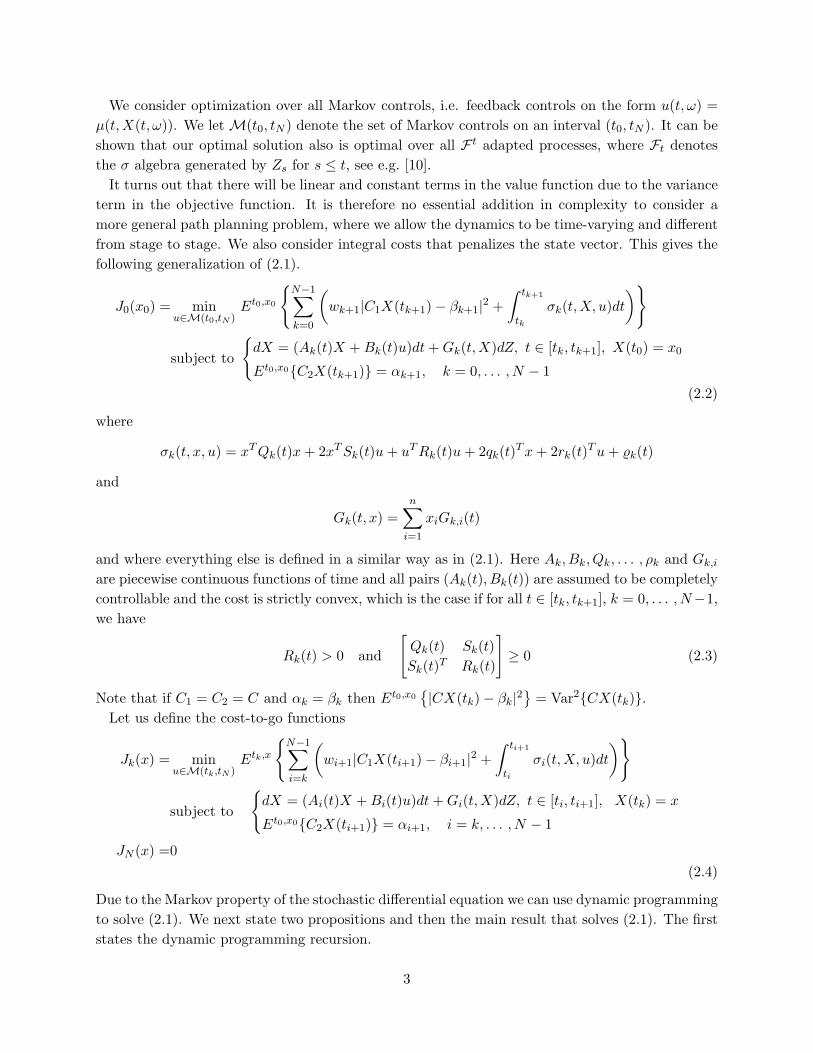
Problem 3.1.

minu

E

{∫ 30

0(u1(t)2 + u2(t)2)dt +

3∑

k=1

wkVar2(Y (10k))

}

subject to the constraints of equation (3.12), (3.13) and (3.15).

We consider the case when wk = 0.01, i = 0.075 and P0 = 105$. In Figure 1 we show a stochasticsimulation of the result. In the upper left plot we show a simulation of the cost value Y . Theupper right plot shows an estimate of the expected value E{Y (t)} obtained by averaging over 1000simulations. The lower left plot shows the controls u1, u2 (u1 in solid line and u2 in dashed line)and the lower right plot shows the P and V (P in solid line and V in dashed line).

0 10 20 300

500

1000

1500

2000Y

0 10 20 300

500

1000

1500

2000EY

0 10 20 30−600

−400

−200

0

200

400

0 10 20 30−1000

−500

0

500

1000

1500

Figure 1: Stochastic simulation of the solution to the investment problem.

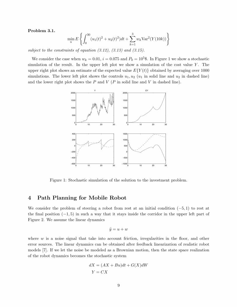
4 Path Planning for Mobile Robot

We consider the problem of steering a robot from rest at an initial condition (−5, 1) to rest atthe final position (−1, 5) in such a way that it stays inside the corridor in the upper left part ofFigure 2. We assume the linear dynamics

y = u + w

where w is a noise signal that take into account friction, irregularities in the floor, and othererror sources. The linear dynamics can be obtained after feedback linearization of realistic robotmodels [7]. If we let the noise be modeled as a Brownian motion, then the state space realizationof the robot dynamics becomes the stochastic system

dX = (AX + Bu)dt + G(X)dW

Y = CX

9

where

A =

0 1 0 00 0 0 00 0 0 10 0 0 0

, B =

0 01 00 00 1

, C =

[1 0 0 00 0 1 0

], G(x) =

0 0x2 00 00 x4

.

Let us use the design equation

−5 −4 −3 −2 −1 0

0

1

2

3

4

5

−5 −4 −3 −2 −1 0

0

1

2

3

4

5

0 2 4 6−3

−2

−1

0

1

2

3

−5 −4 −3 −2 −1 0

0

1

2

3

4

5

Figure 2: The upper left figure shows the initial and final positions for the robot. The upper rightfigure shows one realization of the optimal path of the robot and the lower right figure shows thecorresponding control signals, where u1 corresponds to the solid line and u2 is the dashed line.The weights w1 = 7 and w2 = 1 were used in the optimization problem (4.16). Finally, the lowerright figure shows an estimate of the expected path obtained by averaging over 100 stochasticsimulations.

minE0,x0

{w1|C1X(3) − α1|2 + w2|C3X(6) − α3|2 +

∫ 6

0|u|2dt

}

subj. to

{dX = (AX + Bu)dt + G(X)dW, X(0) = x0

E0,x0 {C2X(3)} = α2, E0,x0 {C3X(6)} = α3

(4.16)

where

C1 =

[1 0 0 00 0 1 0

], α1 =

[−11

]

C2 =[1 0 1 0

], α2 = 0

C3 =

1 0 0 00 1 0 00 0 1 00 0 0 1

, α3 =

−1050

.

10

Stage NStage N−1Stage N−2Stage 2Stage 1Stage 0

Figure 3: We consider optimization of the path from a given initial state at stage 1 to a given nodeαN at stage N . The path must pass trough one node in the graph at each stage.

The idea behind the optimization problem is to divide the control problem into two stages. First,we steer the robot to the switching surface C2x = α2 in such a way that the expected deviationfrom the point C1x = α1 is small. Then in the next stage we steer to the final position x = α3

in such a way that the variance of the deviation from this point is small. The integral cost isintroduced to keep the expected control energy small. With the weights w1 = 7 and w2 = 1 we getthe result in Figure 2. We see from the lower plot that the expected path of the robot stays wellinside the corridor as desired. It is possible to push the trajectory further toward the middle ofthe corridor by adding an integral cost E0,x0

{∫ 60 q|Cx − y0(t)|2dt

}, where q ≥ 0 and y0(t) is some

nominal trajectory near the middle of the corridor. The corresponding optimization problem stillbelongs to the problem class considered in this paper.

5 Route optimization

We can also consider trajectory planning problems where we at each time instant can choose tointerpolate one out of several points. This is illustrated in Figure 3, where we have fixed initialand terminal nodes but can choose between several different routes between these two nodes. Forconsistency with the previous discussion we assume that the initial node is the initial state vector,i.e., α0 = x0. At all other time instants we have a number of possible nodes, each correspondingto a subspace on the form {x ∈ R

n : Cx = αkj}. The nodes at each stage are thus defined by

the set Sk = {αk1 , . . . , αkNk}. We define a set-valued function Nk : Sk �→ P(Sk+1) (P(Sk+1) is

the set of all subsets of Sk+1) that defines the possible successors of each node. This means thatNk(Cxk) ⊂ Sk+1 if Cxk ∈ Sk and Nk(Cxk) = ∅ otherwise. We can now generalize (2.1) and (2.2)to the case when we not only optimize a continuous time trajectory interpolating a given numberof interpolation points (nodes) but also optimize over the set of nodes at each time instant. Let usconsider

J0(x0) = minu∈M(t0,tf )

N−1∑

k=0

(wk+1Var2{CX(tk+1)} + Et0,x0

{∫ tk+1

tk

σk(t, X, u)dt

})

subject to

{dX = (AkX + Bku)dt + Gk(X)dZ, t ∈ [tk, tk+1], X(0) = x0

Et0,x0{CX(tk+1)} ∈ Nk(Et0,x0{CX(tk)}), k = 0, . . . , N − 1

(5.17)

11

For the investment example in the Section 3 this would mean that we can choose between a numberof selected cash values in the intermediate time instances. If we let1

Uk(xk, αk+1) =

{u ∈ M(tk, tk+1) :

{dX = (AkX + Bku)dt + Gk(X)dZ, X(tk) = xk

Etk,xk{CX(tk+1)} = αk+1

}

Ck(u, αk+1) =∫ tk+1

tk

σk(t, X, u)dt + wk+1|CX(tk+1) − αk+1|2

then the dynamic programming iteration for (5.17) can be written as

Jk(xk) = minαk+1∈Nk(Cxk)

minu∈Uk(xk,αk+1)

Etk,xk {Ck(u, αk+1) + Jk+1(X(tk+1))} .

Note that if Cxk �∈ Sk then Nk(Cxk) = ∅ and the optimal objective is unbounded. The solution ofthe inner optimization can be constructed as in Proposition 2.3. We notice that this value functionis completely determined by the node for the case when C = I, i.e. when each node is a point inthe state space of the dynamical system. For this case the route optimization can be performedby discrete dynamic programming iteration over the discrete state space Sk at each stage. Oncewe know the optimal route, i.e., the optimal αk ∈ Sk, k = 1, . . . , N , then we can construct theoptimal control as in Proposition 2.3.

For the general case when C has full row rank m < n, then the problem is much harder becauseJk(xk) is not completely determined by the choice of nodes at stage k, . . . , N . The problem is thencomputationally very expensive for large N . One way to reduce the computational complexity isto discretize the state vector in each node. In this way a suboptimal solution can be obtained bydiscrete dynamic programming. In essense this means that we optimize over a finite collection ofpredefined trajectories, which is an approach that have been discussed for trajectory planning in,for example, [2, 6]. Another way to reduce the complexity is to prune the search tree in someeffiscient way in order to find an optimal (or a near optimal) sequence of nodes. In order to discussthis problem we introduce some new notation. We let αk = (αk, . . . , αN−1, αN ), where αn ∈ Sn,denotes an admissible node sequence from stage k to the terminal fixed node αN , and let

Ak ={αk ∈ ΠN

n=kSn : αn+1 ∈ N (αn)}

be the set of all admissible node sequences from stage k + 1 to the terminal node αN . Similarly

Ak(αk) ={αk+1 ∈ ΠN

n=k+1Sn : αn+1 ∈ N (αn)}

is the set of all sequences of nodes from stage k to stage N with the kth node fixed to be αk. In thesame way as above, the value function in a particular node αk = Cxk at stage k can be computedas

Jk(xk) = minαk+1∈Ak(Cxk)

Jk(xk, αk+1)

We would like to remove as many node sequences as possible from Ak during the dynamic program-ming recursion. Let Ak,O(αk) denote sequences that are candidates for optimality (the index O

1In Ck(u, αk+1) we implicitly assume that X(t) satisfies the stochastic differential equation in the definition of

Uk(xk, αk+1).

12

stands for the open candidates and is a standard notation). Then at each node during the dynamicprogramming recursion we take the following two steps

(i) Ak,O(αk) = {(αk+1, αk+2) : αk+2 ∈ Ak+1,O(αk+1);αk+1 ∈ N (αk)}.

(ii) Remove branches from Ak,O(αk) that cannot correspond to the optimal node sequence.

This gives us the value function Jk(xk) = minαk+1∈Ak,O(αk) Jk(xk, αk+1). The second step is noteasy since each function Jk(xk, αk+1) depends on the particular node sequence αk+1 ∈ Ak+1 butalso on the the state vector at node k which depends on prior stages and in particular the initialcondition. An alternative idea, discussed in for example [8, 9], is to replace step (ii) above with

(ii)′ Remove branches from Ak,O(αk) that are unlikely to be the optimal node sequence.

This generally give suboptimal solutions but the computational complexity may be reduced signif-icantly. Some appealing and promising ideas for implementing (ii)′ was suggested in [8, 9]. Therethey consider optimization of switching sequences for LQR control of switched linear systems. Thisis mathematically closely related to the route optimization considered in this section and theirresults can be adapted to the problem discussed in this section.

Acknowledgement: The research was supported by Grants from the Swedish Research Counciland the NSF.

References

[1] D. P. Bertsekas. Dynamic Programming and Optimal Control, volume 1. Athena Scientific,1995.

[2] M. . Branicky, T. . Johansen, I. Petersen and E. Frazzoli On-line Techniques for BehavioralProgramming In Proceedings of the 39th IEEE Conference on Decision and Control, pages1840-1845, Sydney, Australia, 2000.

[3] P. Crouch and J. W. Jackson. Dynamic interpolation for linear systems. In Proc. 29th IEEEConf. on Decision and Control, pages 2312–2314, Hawaii, 1990.

[4] M. Egerstedt and C. Martin. Optimal trajectory planning and smoothing splines. Automatica,37(7):1057–1064, July 2000.

[5] S.F. Ellermeyer, S.S. Pilyugin and R. Redheffer. Persistence Criteria for a Chemostat withvariable Nutrient Input Journal of differential Equations, 171,132–147 (2001)

[6] E. Frazzoli, M. A. Dahleh and E. Feron A Maneuver-Based Hybrid Control Architecture forAutonomous Vehicle Motion Planning In Software Enabled Control: Information Technologyfor Dynamical Systems, G. Balas and T. Samad editors, 2002. To appear.

[7] J. Lawton, R. Beard and B. Young. A Decentralized Approach To Formation Maneuvers Toappear in IEEE Transactions on Robotics and Automation.

13

[8] B. Lincoln and B. Bernhardsson. Efficient pruning of search trees in LQR control of switchedlinear systems. In Proceedings of the 39th IEEE Conference on Decision and Control, pages1828–1833, Sydney, Australia, 2000.

[9] B. Lincoln and A. Rantzer. Optimizing linear system switching. In Proceedings of the 40thIEEE Conference on Decision and Control, pages 2063–2068, Orlando, FLA, USA, 2001.

[10] B. Øksendal. Stochastic Differential Equations, An Introduction with Applications. Springer,Berlin Heidelberg, fifth edition, 1998.

[11] W. M. Wonham. On a matrix Riccati equation of stochastic control. Siam J. Control Optim.,6(4):681–697, 1968.

[12] Z. Zhang, J. Tomlinson, and C. Martin. Splines and linear control theory. Acta Math. Appl.,49:1–34, 1997.

Appendix A: Proof of Proposition 2.2

We use the compact notation introduced in (2.7) and (2.8) after the proposition. If we apply theLagrange multplier rule to (2.8) then we obtain

V (x0, α, t0, tf ) =maxλ

minu∈M(t0,tf )

Et0,x0

{∫ tf

0[XT QX + 2XT Su + uT Ru]dt

+ X(tf )T Q0X(tf ) + 2λT C(α)X(tf )}

subject to dX = (A(t)X + B(t)u)dt + G(t, X)dZ, X(t0) = x0

The solution to the inner optimization can be obtained from the Hamilton-Jacobi-Bellman Equation(HJBE)

−∂V

∂t= min

u∈Rm

xT Qx + 2xT Su + uT Ru +∂V

∂x

T

(Ax + Bu) +12

n∑

i=1

n∑

j=1

aij∂2V

∂xi∂xj

V (x, tf ) = xT Q0x + 2λT C(α)x

where

aij = (σσT )ij =

((

n∑

k=1

xkGk)(n∑

l=1

xlGTl )

)

ij

=n∑

k,l=1

xkxlGkiGTlj ,

where Gki is the ith row of Gk. With the value function V (x, t) = xT P (t)x we get

12

n∑

i=1

n∑

j=1

aij∂2V

∂xi∂xj=

12

n∑

k=1

n∑

l=1

xkxltr(GTk PGl) = xT Π(P )x,

If we plug the ansatz V (x, t) = xT P (t)x into the HJBE we get the optimal control u = −R−1(BT P+S)x, and that the following Riccati equation must hold

˙P + AT P + P A + Q + Π(P ) = (P B + S)R−1(P B + S)T ,

14

with boundary condition P (tf ) = Q0 + λT Cen+1 + eTn+1C

T λ. The optimal cost becomes

V (x0, α, t0, tf ) =maxλ

xT0 P (λ, t0)x0 (5.18)

To perform the optimization with respect to λ we need to obtain an explicit expression of P as afunction of λ. It turns out that we can use

P = P + NλeTn+1 + en+1λ

T NT − λT Wλen+1eTn+1

where P , N and W are given in (2.7). This follows since

P (tf ) = P (tf ) + N(tf )λeTn+1 + en+1λ

T N(tf )T + λT W (tf )λen+1eTn+1

= Q0 + λT Cen+1 + eTn+1C

T λ

and

˙P = −AT P − P A − Q − Π(P ) + (P B + S)R−1(P B + S)T − (A − BR−1(BT P + ST ))T NλeTn+1

− en+1λT NT (A − BR−1(BT P + ST )) − λT NT BR−1BT Nλen+1e

Tn+1

= −AT P − P A − Q − Π(P ) + (P B + S)R−1(P B + S)T

which follows since

AT (en+1λT NT + λT Wλen+1e

Tn+1) = 0,

BT (en+1λT NT + λT Wλen+1e

Tn+1) = 0.

The optimization in (5.18) thus becomes

maxλ

xT0 (P (t0) + N(t0)λeT

n+1 + en+1λT N(t0)T − λT W (t0)λen+1e

Tn+1)x0

= xT0 (P (t0) + N(t0)W (t0)−1N(t0)T )x0

and the optimal Lagrange multiplier is λ = W (t0)−1N(t0)T x0. Finally, the optimal control becomes

u = −R−1(BT (P + NW (t0)−1N(t0)T x0en+1T ) + S)x

= −R−1(BT P + S)x − R−1BT NW (t0)−1N(t0)T x0

Considering the optimal control problem from the “initial point” (t, x(t)) gives the following feed-back formulation of the optimal control u = −R−1(BT (P + NW−1NT ) + ST )X. We note thatunder the conditions of the proposition there exists solutions P and P to the Riccati equations thatare involved in the proof. Indeed, the special structure of the system matrices imply that only theupper left blocks of P and P satisfy nonlinear equations, which are identical to the first equationin (2.6). The other blocks corresponds to p and ρ in (2.6). Hence, the existence of P and P followsfrom Remark 2.1.

15