![Manipulator trajectory planning - cw.fel.cvut.cz · 17 Non-normalized movement Move the robot from A to B, to run both joints at their maximum angular velocities. After 2 [sec], the](https://static.fdocuments.net/doc/165x107/5e053f85bcd9e654571f0646/manipulator-trajectory-planning-cwfelcvutcz-17-non-normalized-movement-move.jpg)
Trajectory Planning. Goal: to generate the reference inputs to the motion control system which...
57
Trajectory Planning
-
Upload
bryan-bennett -
Category
Documents
-
view
235 -
download
5
Transcript of Trajectory Planning. Goal: to generate the reference inputs to the motion control system which...

Trajectory Planning
Trajectory PlanningTrajectory Planning
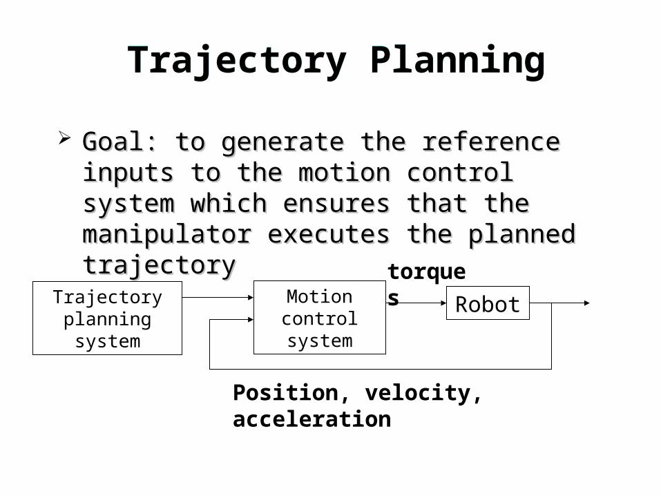
Goal: to generate the reference inputs to the Goal: to generate the reference inputs to the motion control system which ensures that the motion control system which ensures that the manipulator executes the planned trajectorymanipulator executes the planned trajectory
Motion control system
Robot Trajectory planning system
torques
Position, velocity, acceleration

Path and TrajectoryPath and Trajectory
Path: the locus of points in the joint space or in Path: the locus of points in the joint space or in the operational spacethe operational space
Trajectory: a path on which a time law is Trajectory: a path on which a time law is specified in terms of velocities and/or specified in terms of velocities and/or accelerationsaccelerations
t
Path and TrajectoryPath and Trajectory
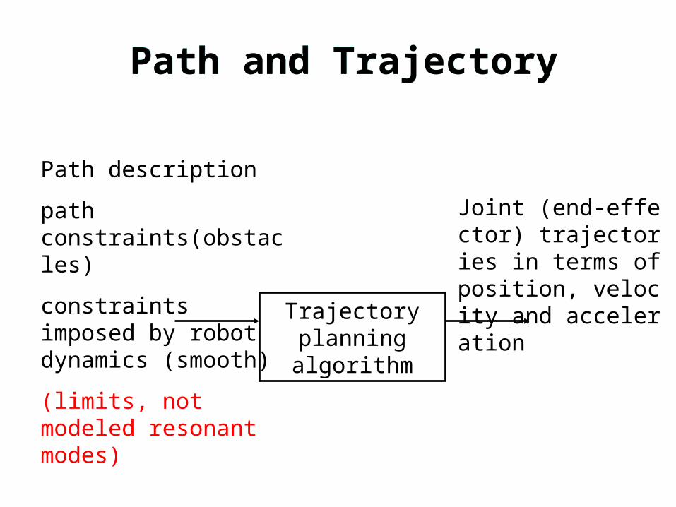
Trajectory planning algorithm
Path description
path constraints(obstacles)
constraints imposed by robot dynamics (smooth)
(limits, not modeled resonant modes)
Joint (end-effector) trajectories in terms of position, velocity and acceleration

Path and TrajectoryPath and Trajectory
Specification of geometric pathSpecification of geometric path Extremal points, possible intermediate points,geomExtremal points, possible intermediate points,geom
etric primitives interpolating the pointsetric primitives interpolating the points
Specification of motion time lawSpecification of motion time law Total trajectory time, maximum velocity and accelerTotal trajectory time, maximum velocity and acceler
ation, velocity and acceleration at points of interestsation, velocity and acceleration at points of interests

Joint Space TrajectoryJoint Space Trajectory
Inverse kinematics algorithm
Trajectory parameters in
operation space
Joint (end-effector) trajectories in terms of position, velocity and acce
leration
Trajectory parameters in joint space Trajectory
planning algorithmInitial and final en
d-effector location, traveling time, etc.
Joint Space TrajectoryJoint Space Trajectory
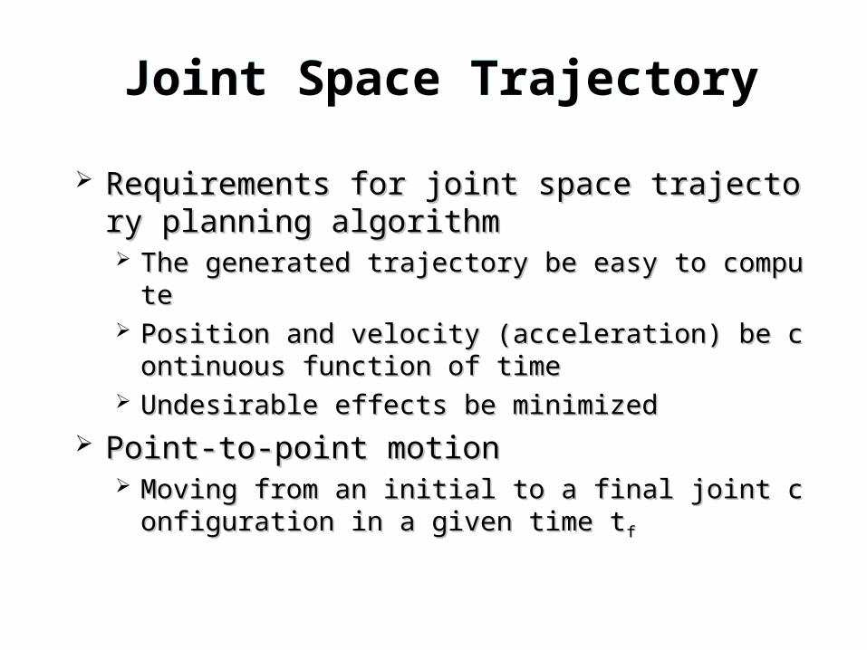
Requirements for joint space trajectory planninRequirements for joint space trajectory planning algorithmg algorithm The generated trajectory be easy to computeThe generated trajectory be easy to compute Position and velocity (acceleration) be continuous fuPosition and velocity (acceleration) be continuous fu
nction of time nction of time Undesirable effects be minimizedUndesirable effects be minimized
Point-to-point motionPoint-to-point motion Moving from an initial to a final joint configuration in Moving from an initial to a final joint configuration in
a given time ta given time tf f
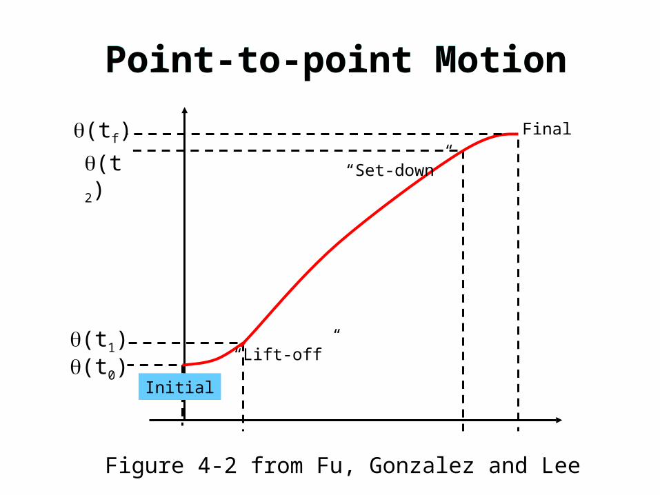
Point-to-point MotionPoint-to-point Motion
Figure 4-2 from Fu, Gonzalez and Lee
(tf)
(t2)
(t0)(t1) “Lift-off”
“Set-down”
Final
Initial

Polynomial interpolationPolynomial interpolation
Example: initial and final position and velocity be Example: initial and final position and velocity be given.given.
Point-to-point MotionPoint-to-point Motion
011
1)( atatatatq nnnn
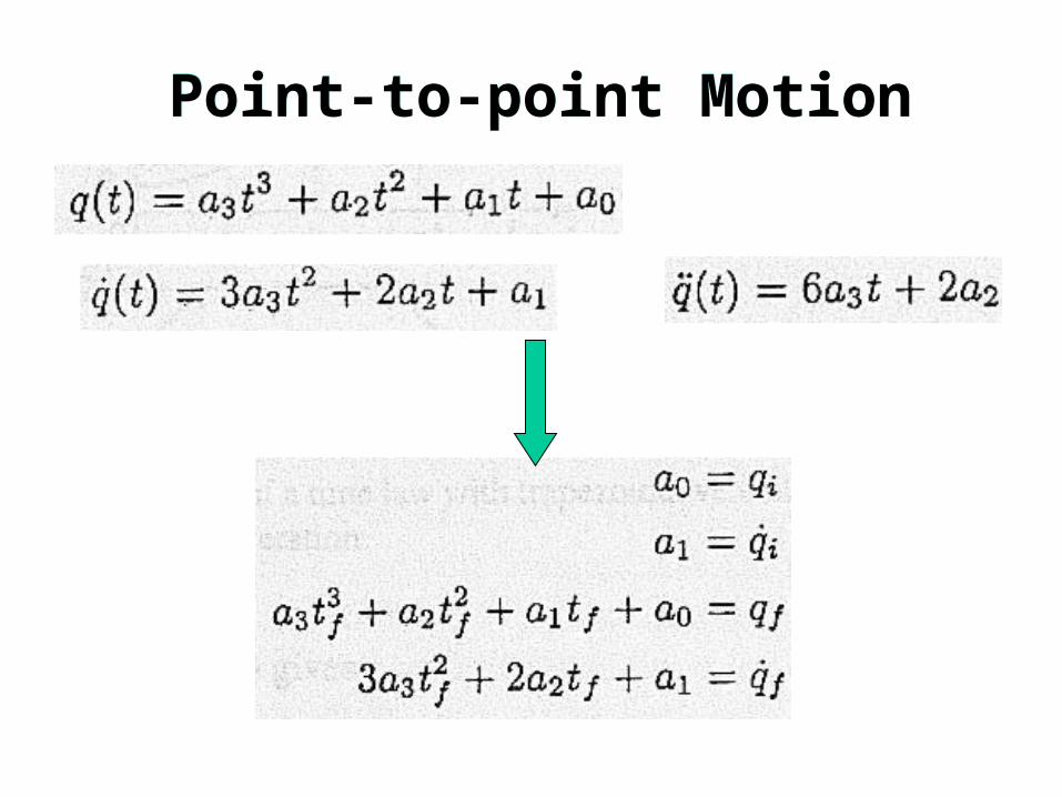
Point-to-point MotionPoint-to-point Motion

Point-to-point MotionPoint-to-point Motion

Example: initial and final acceleration also be Example: initial and final acceleration also be given.given. Six constraints (initial and final position, velocity and Six constraints (initial and final position, velocity and
accelerationacceleration Order at least five Order at least five
Point-to-point MotionPoint-to-point Motion

Trapezoidal velocity profileTrapezoidal velocity profile
Directly verifying whether the velocity and Directly verifying whether the velocity and acceleration violate the mechanical limitsacceleration violate the mechanical limits
Point-to-point MotionPoint-to-point Motion

Area enclosed by the velocity profileArea enclosed by the velocity profile
given accelerationgiven acceleration
Point-to-point MotionPoint-to-point Motion

Point-to-point MotionPoint-to-point Motion
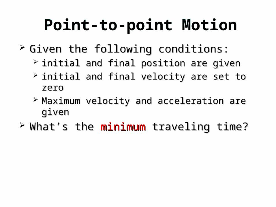
Point-to-point MotionPoint-to-point Motion Given the following conditions:Given the following conditions:
initial and final position are giveninitial and final position are given initial and final velocity are set to zeroinitial and final velocity are set to zero Maximum velocity and acceleration are givenMaximum velocity and acceleration are given
What’s the What’s the minimumminimum traveling time? traveling time?

Path MotionPath Motion Disadvantages of single high order polynomialDisadvantages of single high order polynomial A suitable number of low order polynomialsA suitable number of low order polynomials

Operation Space TrajectoryOperation Space Trajectory Not easy to predict end-effector motion due to kinNot easy to predict end-effector motion due to kin
ematics nonlinearityematics nonlinearity Path motion planning similar to joint spacePath motion planning similar to joint space Different method if the end-effector motion has to Different method if the end-effector motion has to
follow a prescribed trajectory of motion such as linfollow a prescribed trajectory of motion such as line, circle, etc.e, circle, etc.
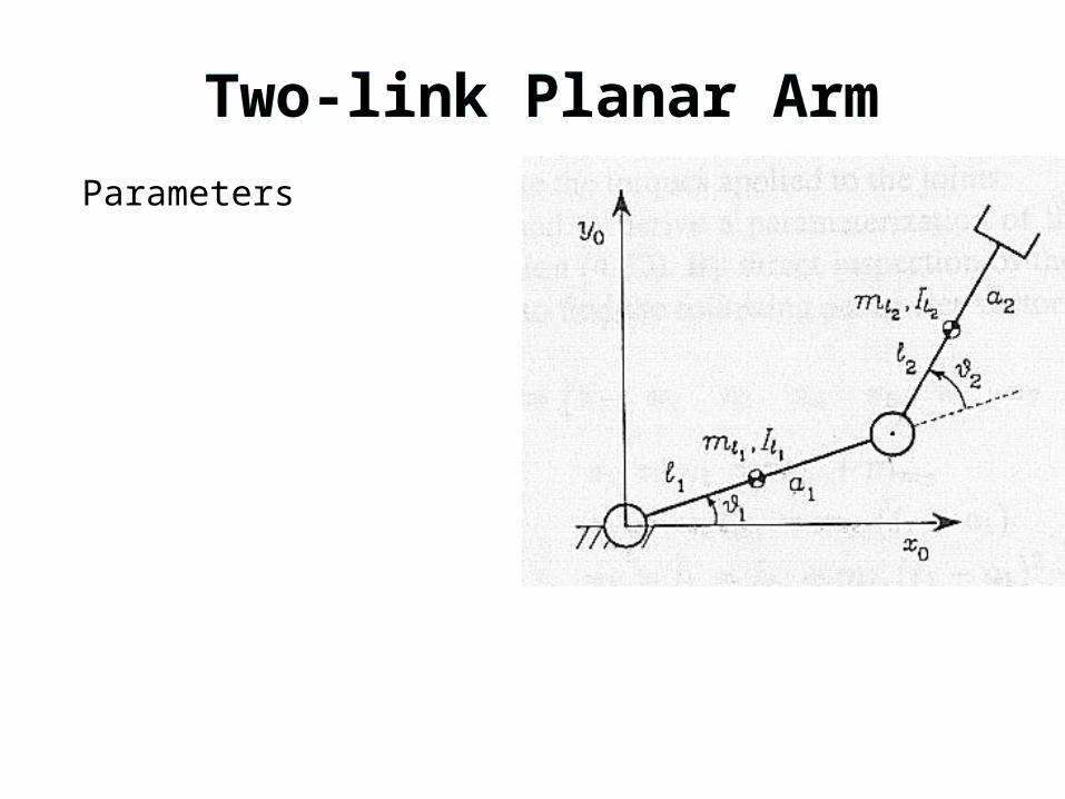
Two-link Planar ArmTwo-link Planar Arm
Parameters

Cams
Motion programming historically Motion programming historically associated with mechanical cams associated with mechanical cams
Constant speed rotation of camshaft Constant speed rotation of camshaft converted to variable linear converted to variable linear displacement of valve (or other device displacement of valve (or other device attached to cam follower) attached to cam follower) – Camshafts in auto engines (all 4 strokes) Camshafts in auto engines (all 4 strokes) – Sewing machine (older mechanical style)Sewing machine (older mechanical style)

Pictures of Cams
http://www.howstuffworks.com/camshaft1.htm
IndustrialIndustrial
Car EnginesCar Engines

Cam Motion Profiles - DRD
Dwell – Rise – Dwell Dwell – Rise – Dwell – initial period of no motion (“dwell”) initial period of no motion (“dwell”) – ““rise” to a maximum displacement rise” to a maximum displacement – final period of no motion (“dwell”)final period of no motion (“dwell”)
“dwell”
“rise”
“dwell”
Time, t
Displacement, s
s=smax, v=0, a=0s=0, v=0, a=0

Cam Motion Profiles - DRRD
Dwell – Rise – Return – Dwell Dwell – Rise – Return – Dwell – initial period of no motion (“dwell”) initial period of no motion (“dwell”) – ““rise” to a maximum displacement rise” to a maximum displacement – Immediately “return” to origin Immediately “return” to origin – final period of no motion (“dwell”)final period of no motion (“dwell”)
“dwell”
“rise”
“dwell”Time, t
Displacement, s s=smax, v=0, a0
s=0, v=0, a=0 “return” s=0, v=0, a=0

Cam Motion Profiles - RR
Rise – Return Rise – Return – ““rise” to a maximum displacement rise” to a maximum displacement – Immediately “return” to origin Immediately “return” to origin – No “dwell” – do same thing over againNo “dwell” – do same thing over again
“rise”
Time, t
Displacement, s s=smax, v=0, a0
“return”s=0, v=0, a0
s=0, v=0, a0

Accel.-Vel.-Disp. #1
Time, t
Acceleration, A Zero order, A = constant
Time, t
Velocity, V
Time, t
Displacement, S
T
T
T
First order, V=k1t
Second order, S=k2t2

Accel.-Vel.-Disp. #1a
Time, t
Acceleration, A
Time, t
Velocity, V
Time, t
Displacement, S
T
T
T
ATV this area
equals this value
2
2
1ATS
this area
equals this value

Accel.-Vel.-Disp. #1b
Time, sec
Acceleration, A
Velocity, V
Displacement, S
T
0 0.1 0.2 0.3
T
25 m/s2
V1V2
V3
S1S2
S3
Find numerical valuesfor V1, V2, and V3
Find numerical valuesfor S1, S2, and S3
Suitable for a “rise”

General Curve Shape: y=Kxn
X
Y
n=1
n=2
n=3
n=4
n=5
1
11
0
1
n
KxdxKxArea
nx n
Area under the curve y=Kxn between x=0 and x=x1 is
Note that y1=Kx1n , so
111111
n
xy
n
xKxArea
n

Accel.-Vel.-Disp. #2
Time, sec
Acceleration, A
Velocity, V
Displacement, S
T
0 0.1 0.2 0.3
T
25 m/s2
V1V2
V3
S1S2
S3
Find numerical valuesfor V1, V2, and V3
Find numerical valuesfor S1, S2, and S3
Suitable for a “dwell - rise”

Accel.-Vel.-Disp. #3
Time, sec
Acceleration, A
Velocity, V
Displacement, S
T
0 0.15 0.3
T
25 m/s2
V1 V2
S1
S2
Find numerical valuesfor V1 and V2
Find numerical valuesfor S1 and S2
Suitable for a “dwell - rise”

Accel.-Vel.-Disp. #4
Time, sec
Acceleration, A
Velocity, V
Displacement, S
T
0 0.1 0.2 0.3
T
25 m/s2
V1V2
V3
S1S2
S3
Find numerical valuesfor V1, V2, and V3
Find numerical valuesfor S1, S2, and S3
Suitable for a “dwell - rise”
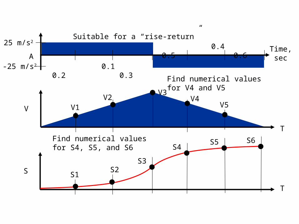
Time, secA
V
S
T
T
25 m/s2
V1V2
V3
S1S2
S3
Find numerical valuesfor V4 and V5
Find numerical valuesfor S4, S5, and S6
Suitable for a “rise-return”
-25 m/s2 0.1 0.2 0.3
0.4 0.5 0.6
V5V4
S4S5 S6

Analytical Solution
Solve the previous problem analytically:Solve the previous problem analytically:
sec6.03.0/25
sec3.00/25)(
2
2
tforsm
tforsmta
0)0(,)()(
0)0(,)()(
0
0
sdttvts
vdttatv
t
t
Hint – solve first parts (for t<0.3 sec), find boundary conditions for 2nd parts

Solve Numerically
Use Excel and trapezoidal integrationUse Excel and trapezoidal integrationtime Acc Vel Disp
0 25 0 00.01 25 0.25 0.001250.02 25 0.5 0.0050.03 25 0.75 0.011250.04 25 1 0.02
sec)03.004.0(*sec
)03.0()04.0(2
1
sec)03.0(
sec)04.0(
2
maa
mv
mv
sec)03.004.0(*sec
)03.0()04.0(2
1)03.0()04.0(
mvvmsms
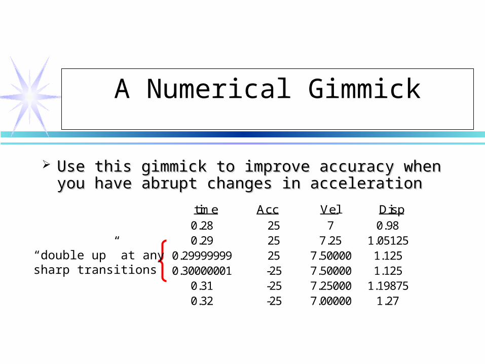
A Numerical Gimmick
Use this gimmick to improve accuracy when Use this gimmick to improve accuracy when you have abrupt changes in accelerationyou have abrupt changes in acceleration
time Acc Vel Disp0 25 0 0
0.01 25 0.25 0.001250.02 25 0.5 0.0050.03 25 0.75 0.011250.04 25 1 0.02
0.28 25 7 0.980.29 25 7.25 1.05125
0.29999999 25 7.50000 1.1250.30000001 -25 7.50000 1.125
0.31 -25 7.25000 1.198750.32 -25 7.00000 1.27
“double up” at anysharp transitions

Motion Programming #2
Robot Joint MotionsRobot Joint Motions

Typical Robot Motion
Figure 4-2 from Fu, Gonzalez and Lee
(tf)
(t2)
(t0)(t1) “Lift-off”
“Set-down”
Final
Initial

Position Constraints
Initial position, Initial position, 1 1
– initial velocity and acceleration (normally=0) initial velocity and acceleration (normally=0)
Lift off position, Lift off position, 22 – velocity and acceleration must match here velocity and acceleration must match here
Set-down position, Set-down position, 33 – velocity and acceleration must match here velocity and acceleration must match here
Final position, Final position, f f
– final velocity and acceleration (normally=0)final velocity and acceleration (normally=0)
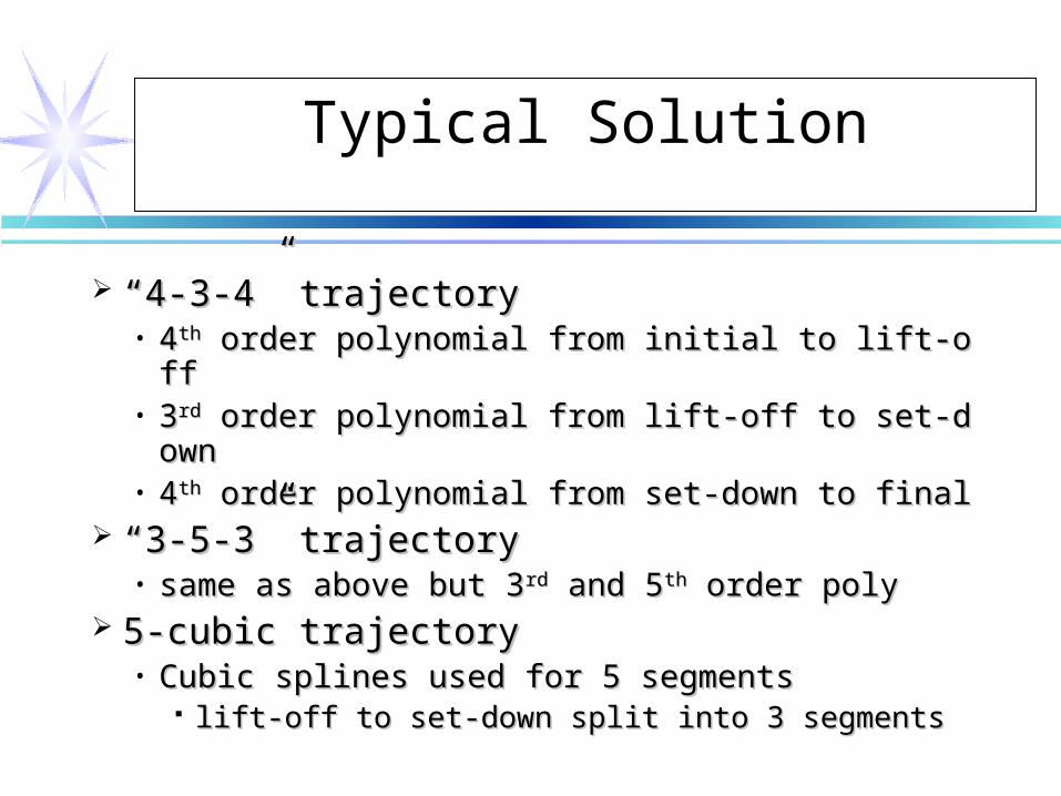
Typical Solution
““4-3-4” trajectory 4-3-4” trajectory • 44thth order polynomial from initial to lift-off order polynomial from initial to lift-off • 33rdrd order polynomial from lift-off to set-down order polynomial from lift-off to set-down • 44thth order polynomial from set-down to final order polynomial from set-down to final
““3-5-3” trajectory 3-5-3” trajectory • same as above but 3same as above but 3rdrd and 5 and 5thth order poly order poly
5-cubic trajectory 5-cubic trajectory • Cubic splines used for 5 segments Cubic splines used for 5 segments
lift-off to set-down split into 3 segments lift-off to set-down split into 3 segments

“4-3-4” Trajectory
11stst segment: segment:
22ndnd segment: segment:
33rdrd segment: segment:
14 unknowns – need 14 equations!14 unknowns – need 14 equations!
10112
123
134
141 )( atatatatath
30312
323
334
343 )( atatatatath
20212
223
232 )( atatatath

Boundary Conditions #1- #3
• 1.1. Initial position, Initial position, 00==(t(t00) (set t) (set t00=0=0
) )
2.2. Initial velocity = Initial velocity = 00 (typically 0) (typically 0)
2.2. 3.3. Initial acceleration = Initial acceleration = 00 (typicall (typicall
y 0) y 0)
1101 )0( ah
1201 2)0( ah
1001 )0( ah

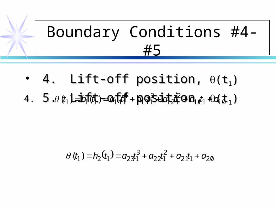
Boundary Conditions #4- #5
• 4.4. Lift-off position, Lift-off position, (t(t11))
4.4. 5.5. Lift-off position, Lift-off position, (t(t11)) 101112112
3113
4114111 )()( atatatatatht
201212122
3123121)( atatatatht
Boundary Conditions #4- #5
• 4.4. Lift-off position, Lift-off position, (t(t11))
4.4. 5.5. Lift-off position, Lift-off position, (t(t11)) 101112112
3113
4114111 )()( atatatatatht
201212122
3123121)( atatatatht

Boundary Conditions #6- #7
• 6.6. Lift-off velocity match from both siLift-off velocity match from both sides des
2.2. 7.7. Lift-off acceleration match both siLift-off acceleration match both sides des
21122212311112
2113
31141211 23234)()( atataatatatathth
221231211321141211 262612)()( ataatatathth

Boundary Conditions #8- #9
• 8.8. Set-down position, Set-down position, (t(t22))
9.9. Set-down position, Set-down position, (t(t22)) 20221
2222
32232 )( atatatat
302312232
3233
42342 )( atatatatat
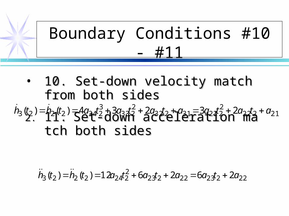
Boundary Conditions #10 - #11
• 10. Set-down velocity match from both 10. Set-down velocity match from both sides sides
2.2. 11.11. Set-down acceleration match botSet-down acceleration match both sides h sides
21222222331232
2233
32342223 23234)()( atataatatatathth
222232222322242223 262612)()( ataatatathth

Boundary Conditions #12- #14
• 12.12. Final position, Final position, (t(tff))
13. Final velocity, v13. Final velocity, vff (typically 0) (typically 0)
2.2. 14.14. Final acceleration, aFinal acceleration, aff (typically 0) (typically 0) 3132
233
3343 234)( atatatath fffff
32332
343 2612)( atatath ffff
30312
323
334
343 )()( atatatatatht ffffff

Solution Format
14 simultaneous linear equations with 14 simultaneous linear equations with 14 unknowns: 14 unknowns:
11 values required to find solution:11 values required to find solution:1011121314 ,,,, aaaaa
3031323334 ,,,, aaaaa20212223 ,,, aaaa
fff
fttttt
,,
,,),(),(
,,
2121
000
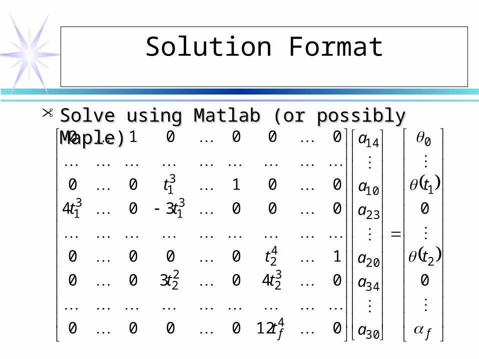
Solution Format
Solve using Matlab (or possibly Maple)Solve using Matlab (or possibly Maple)
ff
t
t
a
a
a
a
a
a
t
tt
t
tt
t
0
0
0120000
040300
10000
000304
00100
000010
2
1
0
30
34
20
23
10
14
4
32
22
42
31
31
31

After Matlab Solution
Once we find the 14 coefficients, how dOnce we find the 14 coefficients, how do we find velocities and accelerations? o we find velocities and accelerations? – Take derivative of hTake derivative of h11(t), h(t), h22(t), h(t), h33(t) to get vel(t) to get vel
ocity ocity – Take derivative of velocity to get accel. Take derivative of velocity to get accel. – Both are easily plotted in Matlab or ExcelBoth are easily plotted in Matlab or Excel

Problems
What if the velocities or accelerations wWhat if the velocities or accelerations we find are too large? e find are too large? – Increase times tIncrease times t11, t, t22, t, tf f
– Move the pick-up point closer to Move the pick-up point closer to (t(t00) )
– Move the drop-off point closer to Move the drop-off point closer to (t(tff))

Motion Programming #3
Friday, October 19, 2001Friday, October 19, 2001

Plan Motion Program
X0
Y0
x0
y0
0
Y1
X1
0
x2
a1
v
vv
v
R
a2
y2
from
1
0
40
1
y
x
R 0
0
0 cm
cm
to
1
30
40
1
y
x
R 0
0
cm
cm
f
a1 = 60 cm, a2 = 40 cm,
x2 = 5 cm, y2 = 5 cm
1,max = 2,max = 6 rad/sec,
1,max = 2,max = 20 rad/sec2

Inverse Kinematics
What is the minimum time T that meets What is the minimum time T that meets velocity and acceleration constraints for velocity and acceleration constraints for both joints?both joints?
x0 y0 1 2 1 240 0 0.855 3.761 48.99 215.4740 30 1.473 3.983 84.42 228.23
cm radians degrees
from Inverse Kinematics:

Motion Programming #1
• Work in groups of 2: Work in groups of 2: Determine an “S” curve for Determine an “S” curve for each joint each joint Need something suitable for DRD Need something suitable for DRD
motion motion Turn in solution Turn in solution
• will have two groups show solution will have two groups show solution
Use T = 1.0 second as a “reasonable” timeUse T = 1.0 second as a “reasonable” time

Straight-Line Motion
Define 10 “knot” points along the straight line Define 10 “knot” points along the straight line Find inverse kinematic solution at each point:Find inverse kinematic solution at each point:
x0 y0 1 2 1 240 0 0.855 3.761 48.99 215.4740 3 0.930 3.763 53.27 215.6140 6 1.004 3.770 57.50 216.0340 9 1.076 3.783 61.63 216.7340 12 1.145 3.799 65.60 217.7040 15 1.211 3.821 69.38 218.9140 18 1.273 3.846 72.93 220.3640 21 1.330 3.875 76.22 222.0440 24 1.383 3.908 79.23 223.9140 27 1.431 3.944 81.97 225.9840 30 1.473 3.983 84.42 228.23
degreescm radians

Motion Programming #2
Select T = 1 second as a “reasonable” Select T = 1 second as a “reasonable” time for complete straight line motion time for complete straight line motion
Work in groups of 2: Work in groups of 2:
Are there any constraints that need to be Are there any constraints that need to be considered? What do you recommend to considered? What do you recommend to determine desired positions at intermediate determine desired positions at intermediate times? times?