
Trajectory Optimization for Manipulation of Deformable ...
7
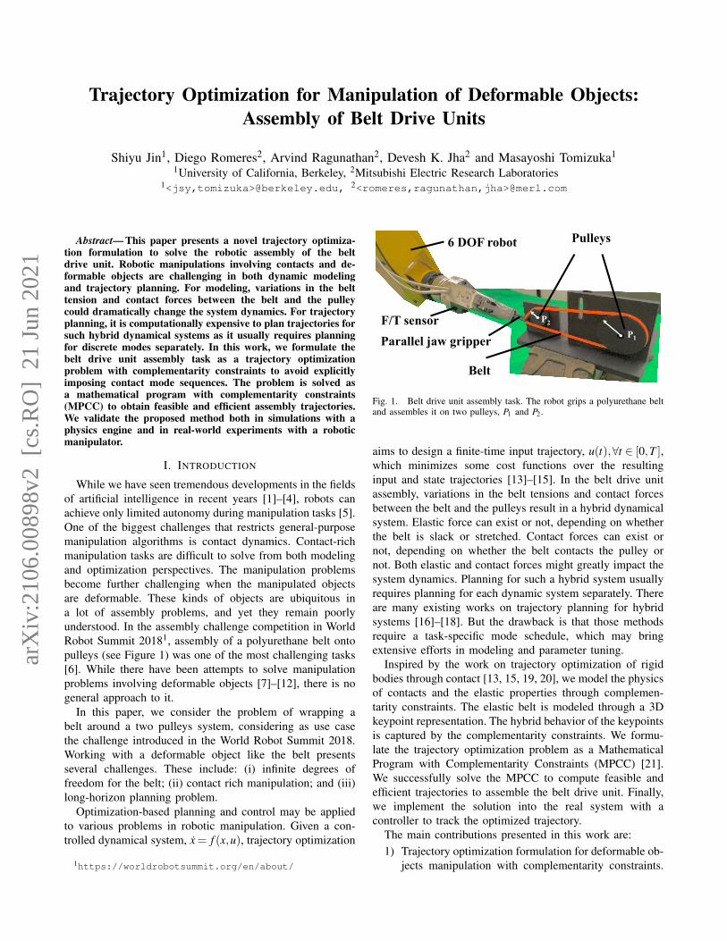
Trajectory Optimization for Manipulation of Deformable Objects: Assembly of Belt Drive Units Shiyu Jin 1 , Diego Romeres 2 , Arvind Ragunathan 2 , Devesh K. Jha 2 and Masayoshi Tomizuka 1 1 University of California, Berkeley, 2 Mitsubishi Electric Research Laboratories 1 <jsy,tomizuka>@berkeley.edu, 2 <romeres,ragunathan,jha>@merl.com Abstract— This paper presents a novel trajectory optimiza- tion formulation to solve the robotic assembly of the belt drive unit. Robotic manipulations involving contacts and de- formable objects are challenging in both dynamic modeling and trajectory planning. For modeling, variations in the belt tension and contact forces between the belt and the pulley could dramatically change the system dynamics. For trajectory planning, it is computationally expensive to plan trajectories for such hybrid dynamical systems as it usually requires planning for discrete modes separately. In this work, we formulate the belt drive unit assembly task as a trajectory optimization problem with complementarity constraints to avoid explicitly imposing contact mode sequences. The problem is solved as a mathematical program with complementarity constraints (MPCC) to obtain feasible and efficient assembly trajectories. We validate the proposed method both in simulations with a physics engine and in real-world experiments with a robotic manipulator. I. I NTRODUCTION While we have seen tremendous developments in the fields of artificial intelligence in recent years [1]–[4], robots can achieve only limited autonomy during manipulation tasks [5]. One of the biggest challenges that restricts general-purpose manipulation algorithms is contact dynamics. Contact-rich manipulation tasks are difficult to solve from both modeling and optimization perspectives. The manipulation problems become further challenging when the manipulated objects are deformable. These kinds of objects are ubiquitous in a lot of assembly problems, and yet they remain poorly understood. In the assembly challenge competition in World Robot Summit 2018 1 , assembly of a polyurethane belt onto pulleys (see Figure 1) was one of the most challenging tasks [6]. While there have been attempts to solve manipulation problems involving deformable objects [7]–[12], there is no general approach to it. In this paper, we consider the problem of wrapping a belt around a two pulleys system, considering as use case the challenge introduced in the World Robot Summit 2018. Working with a deformable object like the belt presents several challenges. These include: (i) infinite degrees of freedom for the belt; (ii) contact rich manipulation; and (iii) long-horizon planning problem. Optimization-based planning and control may be applied to various problems in robotic manipulation. Given a con- trolled dynamical system, ˙ x = f (x, u), trajectory optimization 1 https://worldrobotsummit.org/en/about/ 6 DOF robot F/T sensor Parallel jaw gripper Pulleys Belt P 2 P 1 Fig. 1. Belt drive unit assembly task. The robot grips a polyurethane belt and assembles it on two pulleys, P 1 and P 2 . aims to design a finite-time input trajectory, u(t ), ∀t ∈ [0, T ], which minimizes some cost functions over the resulting input and state trajectories [13]–[15]. In the belt drive unit assembly, variations in the belt tensions and contact forces between the belt and the pulleys result in a hybrid dynamical system. Elastic force can exist or not, depending on whether the belt is slack or stretched. Contact forces can exist or not, depending on whether the belt contacts the pulley or not. Both elastic and contact forces might greatly impact the system dynamics. Planning for such a hybrid system usually requires planning for each dynamic system separately. There are many existing works on trajectory planning for hybrid systems [16]–[18]. But the drawback is that those methods require a task-specific mode schedule, which may bring extensive efforts in modeling and parameter tuning. Inspired by the work on trajectory optimization of rigid bodies through contact [13, 15, 19, 20], we model the physics of contacts and the elastic properties through complemen- tarity constraints. The elastic belt is modeled through a 3D keypoint representation. The hybrid behavior of the keypoints is captured by the complementarity constraints. We formu- late the trajectory optimization problem as a Mathematical Program with Complementarity Constraints (MPCC) [21]. We successfully solve the MPCC to compute feasible and efficient trajectories to assemble the belt drive unit. Finally, we implement the solution into the real system with a controller to track the optimized trajectory. The main contributions presented in this work are: 1) Trajectory optimization formulation for deformable ob- jects manipulation with complementarity constraints. arXiv:2106.00898v2 [cs.RO] 21 Jun 2021
Transcript of Trajectory Optimization for Manipulation of Deformable ...
Trajectory Optimization for Manipulation of Deformable Objects:Assembly of Belt Drive Units
Shiyu Jin1, Diego Romeres2, Arvind Ragunathan2, Devesh K. Jha2 and Masayoshi Tomizuka1
1University of California, Berkeley, 2Mitsubishi Electric Research Laboratories1<jsy,tomizuka>@berkeley.edu, 2<romeres,ragunathan,jha>@merl.com
Abstract— This paper presents a novel trajectory optimiza-tion formulation to solve the robotic assembly of the beltdrive unit. Robotic manipulations involving contacts and de-formable objects are challenging in both dynamic modelingand trajectory planning. For modeling, variations in the belttension and contact forces between the belt and the pulleycould dramatically change the system dynamics. For trajectoryplanning, it is computationally expensive to plan trajectories forsuch hybrid dynamical systems as it usually requires planningfor discrete modes separately. In this work, we formulate thebelt drive unit assembly task as a trajectory optimizationproblem with complementarity constraints to avoid explicitlyimposing contact mode sequences. The problem is solved asa mathematical program with complementarity constraints(MPCC) to obtain feasible and efficient assembly trajectories.We validate the proposed method both in simulations with aphysics engine and in real-world experiments with a roboticmanipulator.
I. INTRODUCTION
While we have seen tremendous developments in the fieldsof artificial intelligence in recent years [1]–[4], robots canachieve only limited autonomy during manipulation tasks [5].One of the biggest challenges that restricts general-purposemanipulation algorithms is contact dynamics. Contact-richmanipulation tasks are difficult to solve from both modelingand optimization perspectives. The manipulation problemsbecome further challenging when the manipulated objectsare deformable. These kinds of objects are ubiquitous ina lot of assembly problems, and yet they remain poorlyunderstood. In the assembly challenge competition in WorldRobot Summit 20181, assembly of a polyurethane belt ontopulleys (see Figure 1) was one of the most challenging tasks[6]. While there have been attempts to solve manipulationproblems involving deformable objects [7]–[12], there is nogeneral approach to it.
In this paper, we consider the problem of wrapping abelt around a two pulleys system, considering as use casethe challenge introduced in the World Robot Summit 2018.Working with a deformable object like the belt presentsseveral challenges. These include: (i) infinite degrees offreedom for the belt; (ii) contact rich manipulation; and (iii)long-horizon planning problem.
Optimization-based planning and control may be appliedto various problems in robotic manipulation. Given a con-trolled dynamical system, x = f (x,u), trajectory optimization
1https://worldrobotsummit.org/en/about/
6 DOF robot
F/T sensorParallel jaw gripper
Pulleys
Belt
P2
P1
Fig. 1. Belt drive unit assembly task. The robot grips a polyurethane beltand assembles it on two pulleys, P1 and P2.
aims to design a finite-time input trajectory, u(t),∀t ∈ [0,T ],which minimizes some cost functions over the resultinginput and state trajectories [13]–[15]. In the belt drive unitassembly, variations in the belt tensions and contact forcesbetween the belt and the pulleys result in a hybrid dynamicalsystem. Elastic force can exist or not, depending on whetherthe belt is slack or stretched. Contact forces can exist ornot, depending on whether the belt contacts the pulley ornot. Both elastic and contact forces might greatly impact thesystem dynamics. Planning for such a hybrid system usuallyrequires planning for each dynamic system separately. Thereare many existing works on trajectory planning for hybridsystems [16]–[18]. But the drawback is that those methodsrequire a task-specific mode schedule, which may bringextensive efforts in modeling and parameter tuning.
Inspired by the work on trajectory optimization of rigidbodies through contact [13, 15, 19, 20], we model the physicsof contacts and the elastic properties through complemen-tarity constraints. The elastic belt is modeled through a 3Dkeypoint representation. The hybrid behavior of the keypointsis captured by the complementarity constraints. We formu-late the trajectory optimization problem as a MathematicalProgram with Complementarity Constraints (MPCC) [21].We successfully solve the MPCC to compute feasible andefficient trajectories to assemble the belt drive unit. Finally,we implement the solution into the real system with acontroller to track the optimized trajectory.
The main contributions presented in this work are:1) Trajectory optimization formulation for deformable ob-
jects manipulation with complementarity constraints.
arX
iv:2
106.
0089
8v2
[cs
.RO
] 2
1 Ju
n 20
21
This provides a general-purpose, mathematical frame-work to tackle these problems.
2) Introduction of 3D keypoint representation for de-formable objects.
3) Validation of the proposed approach through simula-tion as well as real experiments.
II. RELATED WORK
Deformable linear (one-dimensional) object manipulationhas been studied for decades. A randomized algorithm wasproposed to plan a collision-free path for elastic objects[22]. Minimal-energy curves were applied to plan paths fordeformable linear objects in stable configurations [23]. In[24], a local deformation model approximation method wasproposed to control the soft objects to desired shapes. Theauthors of [25, 26] extended the local deformation modelto the manipulation of cables. A deep neural network wastrained to manipulate a rope to target shape based on asequence of images [27]. However, those works do notconsider the interaction between the deformable cables andthe environment. In [7], the authors proposed a strategy toassemble a flexible beam into a rigid hole. An optimization-based trajectory planning was utilized to assembly ring-shaped elastic objects in [8], but the authors only validatedtheir method in simulation. In [9], the authors took theadvantage of environmental contacts to shape deformablelinear objects by a vision-based contact detector. The authorsof [10] considered a scenario to assemble the roller chainto sprockets. Their strategy successfully assemble the chainbut lacks in generalization because each step is engineeredfor the specific system. To advance the research on roboticmanipulation, the World Robot Summit 2018 proposed acompetition on assembly challenges [6]. The challenge high-lighted the complexity of solving manipulation tasks in ageneral manner, which still remains an open problem.
Optimization-based methods have been successfully im-plemented in many trajectory planning scenarios [28]–[30].[13] proposed a trajectory optimization method for rigidbodies contacting the environment. They formulated anMPCC to eliminate the prior mode ordering in discontinuousdynamics due to inelastic impacts and Coulomb friction. TheMPCC framework was extended to a quadrotor with a cable-suspended payload system in [31]. The complementarityconstraint was utilized to model the limitation of a non-stretchable cable length. Inspired by [13, 15, 19, 20, 31],we introduce complementarity constraints to the belt driveunit assembly task to avoid the hybrid modes selection dueto elastic force in the belt and contact force between thebelt and the pulleys. We extend the keypoints representationintroduced for rigid objects, [32], to model elastic objects likethe belt and to formulate an MPCC to perform the assembly.
III. PROBLEM FORMULATION
The belt drive unit consists of two pulleys attached toa base and of a deformable and stretchable belt as shownin Figure 1. The belt is assumed to be composed of ahomogeneous isotropic linear elastic material which is a
K1
K2
L
XY
Z Roll
Pitch
Yaw
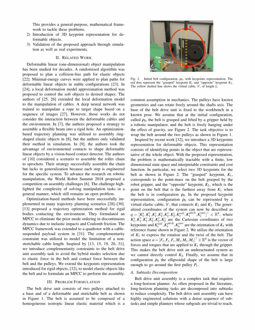
Fig. 2. Initial belt configuration, ρ0, with keypoints representation. Thered dots represent the “grasped” keypoint K1 and “opposite” keypoint K2.The yellow dashed line shows the virtual cable, C , of length L.
common assumption in mechanics. The pulleys have knowngeometries and can rotate freely around the shafts axis. Thebase of the belt drive unit is fixed to the workbench in aknown pose. We assume that at the initial configuration,called ρ0, the belt is grasped and lifted by a gripper held bya robotic manipulator, and the belt is freely hanging underthe effect of gravity, see Figure 2. The task objective is towrap the belt around the two pulleys as shown in Figure 1.
Inspired by recent work [32], we introduce a 3D keypointsrepresentation for deformable objects. This representationconsists of identifying points in the object that are represen-tative of the whole object. With the proposed representation,the problem is mathematically tractable with a finite, lowdimensional state space and interpretable constraints and costfunction. In particular, we select two 3D keypoints for thebelt as shown in Figure 2. The “grasped” keypoint, K1,corresponds to the point-mass on the belt grasped by therobot gripper, and the “opposite” keypoint, K2, which is thepoint on the belt that is the furthest away from K1 whenthe belt is in configuration ρ0. In the proposed keypointrepresentation, configuration ρ0 can be represented by avirtual elastic cable, C , that connects K1 and K2. The gener-alized coordinates of the system can now be described asq = [Kx
1 ,Ky1 ,K
z1,K
x2 ,K
y2 ,K
z2,K
roll1 ,K pitch
1 ,Kyaw1 ]> ∈ R9, where
Kx1 ,K
y1 ,K
z1,K
x2 ,K
y2 ,K
z2 are the Cartesian coordinates of two
keypoints and Kroll1 ,K pitch
1 ,Kyaw1 are the orientation of K1 with
reference frame shown in Figure 2. We utilize the orientationof K1 to express the rotation and the twist of the belt. Theaction space u= [Fx,Fy,Fz,Mx,My,Mz]
> ∈R6 is the vector offorces and torques that are applied to K1 through the gripper.This makes the belt drive unit an underactuated system aswe cannot directly control K2. Finally, we assume that inconfiguration ρ0 the ellipsoidal shape of the belt is largeenough to go around the first pulley P1.
A. Subtasks Decomposition
Belt drive unit assembly is a complex task that requiresa long-horizon planner. As often proposed in the literature,long-horizon planning tasks are decomposed into subtasksto reduce complexity. The belt drive unit assembly can havehighly engineered solutions with a dense sequence of sub-tasks and simple planners whose subgoals are trivial to reach.
K1
K2K1
K2P1 P1P2P2
S1 S2
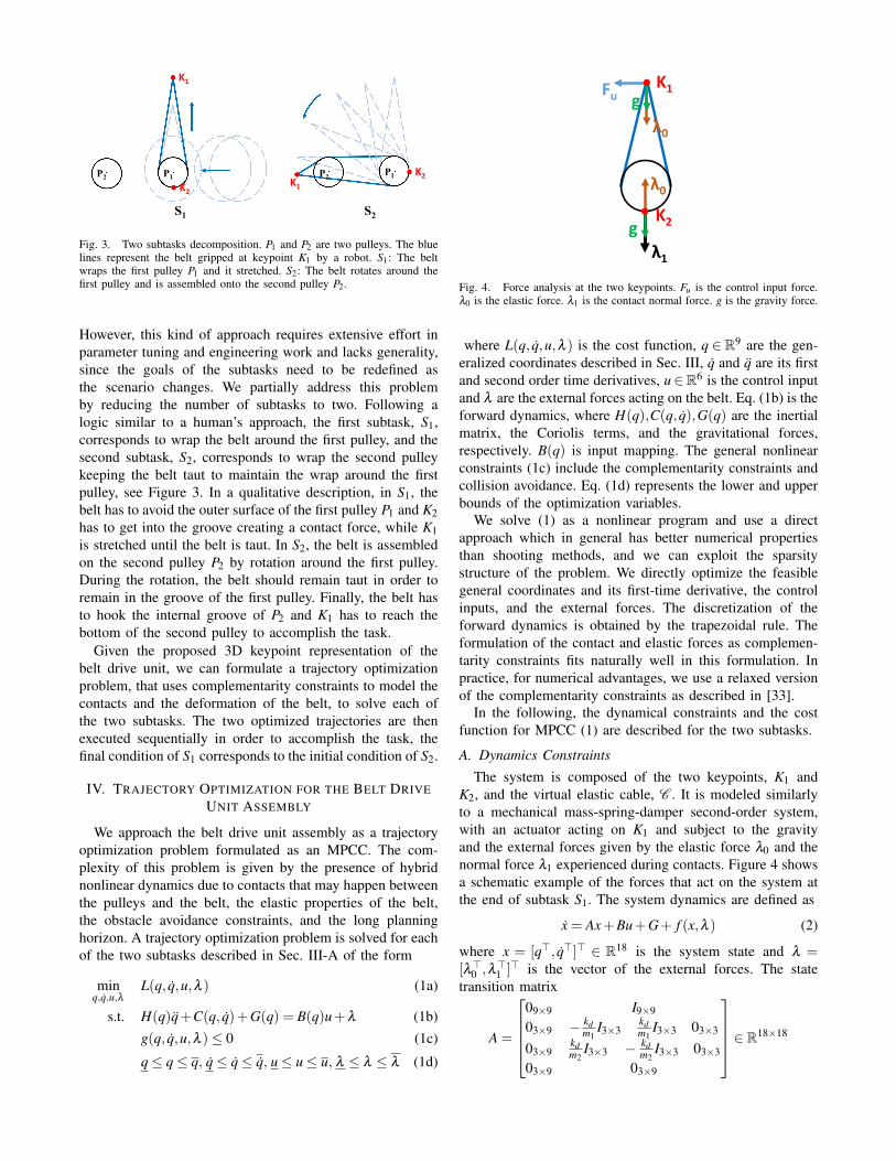
Fig. 3. Two subtasks decomposition. P1 and P2 are two pulleys. The bluelines represent the belt gripped at keypoint K1 by a robot. S1: The beltwraps the first pulley P1 and it stretched. S2: The belt rotates around thefirst pulley and is assembled onto the second pulley P2.
However, this kind of approach requires extensive effort inparameter tuning and engineering work and lacks generality,since the goals of the subtasks need to be redefined asthe scenario changes. We partially address this problemby reducing the number of subtasks to two. Following alogic similar to a human’s approach, the first subtask, S1,corresponds to wrap the belt around the first pulley, and thesecond subtask, S2, corresponds to wrap the second pulleykeeping the belt taut to maintain the wrap around the firstpulley, see Figure 3. In a qualitative description, in S1, thebelt has to avoid the outer surface of the first pulley P1 and K2has to get into the groove creating a contact force, while K1is stretched until the belt is taut. In S2, the belt is assembledon the second pulley P2 by rotation around the first pulley.During the rotation, the belt should remain taut in order toremain in the groove of the first pulley. Finally, the belt hasto hook the internal groove of P2 and K1 has to reach thebottom of the second pulley to accomplish the task.
Given the proposed 3D keypoint representation of thebelt drive unit, we can formulate a trajectory optimizationproblem, that uses complementarity constraints to model thecontacts and the deformation of the belt, to solve each ofthe two subtasks. The two optimized trajectories are thenexecuted sequentially in order to accomplish the task, thefinal condition of S1 corresponds to the initial condition of S2.
IV. TRAJECTORY OPTIMIZATION FOR THE BELT DRIVEUNIT ASSEMBLY
We approach the belt drive unit assembly as a trajectoryoptimization problem formulated as an MPCC. The com-plexity of this problem is given by the presence of hybridnonlinear dynamics due to contacts that may happen betweenthe pulleys and the belt, the elastic properties of the belt,the obstacle avoidance constraints, and the long planninghorizon. A trajectory optimization problem is solved for eachof the two subtasks described in Sec. III-A of the form
minq,q,u,λ
L(q, q,u,λ ) (1a)
s.t. H(q)q+C(q, q)+G(q) = B(q)u+λ (1b)g(q, q,u,λ )≤ 0 (1c)
q≤ q≤ q, q≤ q≤ q, u≤ u≤ u, λ ≤ λ ≤ λ (1d)
K1
K2
u
g
Fk
λ1
λ1
λ0
λ0
g
g
Fu
Fig. 4. Force analysis at the two keypoints. Fu is the control input force.λ0 is the elastic force. λ1 is the contact normal force. g is the gravity force.
where L(q, q,u,λ ) is the cost function, q ∈ R9 are the gen-eralized coordinates described in Sec. III, q and q are its firstand second order time derivatives, u∈R6 is the control inputand λ are the external forces acting on the belt. Eq. (1b) is theforward dynamics, where H(q),C(q, q),G(q) are the inertialmatrix, the Coriolis terms, and the gravitational forces,respectively. B(q) is input mapping. The general nonlinearconstraints (1c) include the complementarity constraints andcollision avoidance. Eq. (1d) represents the lower and upperbounds of the optimization variables.
We solve (1) as a nonlinear program and use a directapproach which in general has better numerical propertiesthan shooting methods, and we can exploit the sparsitystructure of the problem. We directly optimize the feasiblegeneral coordinates and its first-time derivative, the controlinputs, and the external forces. The discretization of theforward dynamics is obtained by the trapezoidal rule. Theformulation of the contact and elastic forces as complemen-tarity constraints fits naturally well in this formulation. Inpractice, for numerical advantages, we use a relaxed versionof the complementarity constraints as described in [33].
In the following, the dynamical constraints and the costfunction for MPCC (1) are described for the two subtasks.
A. Dynamics ConstraintsThe system is composed of the two keypoints, K1 and
K2, and the virtual elastic cable, C . It is modeled similarlyto a mechanical mass-spring-damper second-order system,with an actuator acting on K1 and subject to the gravityand the external forces given by the elastic force λ0 and thenormal force λ1 experienced during contacts. Figure 4 showsa schematic example of the forces that act on the system atthe end of subtask S1. The system dynamics are defined as
x = Ax+Bu+G+ f (x,λ ) (2)
where x = [q>, q>]> ∈ R18 is the system state and λ =[λ>0 ,λ>1 ]> is the vector of the external forces. The statetransition matrix
A =
09×9 I9×9
03×9 − kdm1
I3×3kdm1
I3×3 03×3
03×9kdm2
I3×3 − kdm2
I3×3 03×3
03×9 03×9
∈ R18×18

represents the effect of the mass-spring-damper system withkd the damping coefficient and m1, m2 are the masses of thekeypoints K1 and K2, respectively. The input matrix
B =
09×6
I3×3m1
03×3
03×6
03×3I3×3M1
∈ R18×6
maps the 6-dimensional end-effector force/torque input u tothe linear and angular acceleration of the “grasped” keypointK1. M1 is the moment of inertia of K1. The gravitationalacceleration is applied to the two keypoints through thevector G =
[01×11,−g, 01×2,−g, 01×3
]> ∈ R18×1.The contribution of the external forces is now given by
the sum of the elastic and normal force f (x,λ ) = λ0 +λ1.The elastic force is defined as
λ0 =[03×9,− I3×3
m1,
I3×3m2
, 03×3
]>ΠK1,p λ0 ∈ R18×1
where λ0 ∈ R is the magnitude of the elastic force and isthe variable optimized, ΠK1,p =
[(Kx1−px),(Ky
1−py),(Kz1−pz)]>
||K1−p|| isthe projection operator of the elastic force into the 3 axis.The point p is K2 in S1 and O1 in S2 for simplicity ofcomputation. O1 is the position of the first pulley’s center.The normal force due to the contacts between the pulley andthe keypoint K2 is defined as
λ1 =[03×12,− I3×3
m2, 03×3
]>ΠO1,K2 λ1 ∈ R18×1
where λ1 ∈R is the magnitude of the normal force and is thevariable optimized and ΠO1,K2 =
[(ox1−Kx
2),(oy1−Ky
2),(oz1−Kz
2)]>
||o1−K2||is
the projection operator of the normal force into the 3-axis.
B. Complementarity Constraints
In order to model the hybrid dynamics due to elastic forceand contact force, we use complementarity constraints
0≤ g(·) ⊥ h(·)≥ 0 (3)
Complementary constraints are a way to model constraintsthat are combinatorial in nature and impose the positivityand orthogonality of the variables.
Elastic force constraint. The first complementarity con-straint is formulated as
λ2 =λ0
kp+L− l(x)≥ 0 (4a)
λ0 ≥ 0 (4b)
λ0λ2 = 0 (4c)
where L and kp are respectively the length at configurationρ0 and the stiffness coefficient of the virtual elastic cable, C .The length of C at each temporal instant is l(x) = ||K1−K2||in S1, and l(x) = ||K1−O1||+ r1 in S2, where r1 denotes theradius of P1. The pulley center O1 is chosen because it is afixed known point while the pulley is rotating. From eq. (4a)the elasticity of the belt is defined as proportional to thelength L− l(x) and depends on the stiffness coefficient kp.
λ2 is an algebraic variable. If the cable is stretched, thenL < l(x), λ0 > 0, and λ2 = 0. If the cable is slack, thenL > l(x), λ0 = 0, and λ2 > 0.
Contact force constraint. The second complementarityconstraint is formulated as
λ3 =√||K2−Oe||2 + ε2 ≥ ε (5a)
λ1 ≥ 0 (5b)
λ1λ3 = 0 (5c)
where Oe is the contact point on the edge of P1. ε denotes asmall number to relax the complementarity constraint [33].λ3 is the algebraic variable describes whether the belt con-tacts the pulley. If the belt contacts the pulley, then λ3 = ε ,and contact force λ1 ≥ 0. If there is no contact, then λ3 > ε ,and contact force λ1 = 0.
C. Obstacle avoidance
This constraint imposes that the keypoints cannot pen-etrate into the pulleys. Each pulley is approximatedwith an ellipsoid, since there is a known analytical ex-pression of the distance function between a point andan ellipsoid. The obstacle avoidance constraints betweena keypoint Ki and a pulley Pj can be denoted as
distance(Ki,Pj) =√
(Ki−O j)>S(Ki−O j)− 1 ≥ 0, whereS = diag{1/a2,1/b2,1/c2} is a diagonal matrix, a,b,c arehalf the length of the principal axes. O j denotes the centerof pulley Pj.
D. Physics Limitation
The belt might break if stretched over a certain limit, thiscondition is approximated by constraining the length of thevirtual cable C , l(x)≤ Lmax. Moreover, Lmax is assumed largeenough for the loop to go around two pulleys.
E. Cost Function
We use a common quadratic cost function that penalizesthe difference to the goal state xgoal and the control in-put u(k):
J(x,u,λ ) =N
∑k=0
(x(k)− xgoal)>Q(x(k)− xgoal)+
u(k)T Ru(k)+w(λ0(k)− λdesired0 )2
(6)
where the weights Q and R are diagonal matrices and w isa scalar. Moreover, the term w(λ0(k)− λ desired
0 )2 adds a softconstraint in the elastic force. A positive λ desired
0 encouragesa solution with the belt in tension. This constraint is usedin subtask S2 to maintain the belt taut. Instead, in S1 we setw = 0.
V. EXPERIMENTAL RESULTS
In this section, we present the results of the proposedmethod both in simulation using the physic engine Mu-JoCo [34] and in a real system with a 6-DoF manipulator.We use the Ipopt [35] solver in a python wrapper.
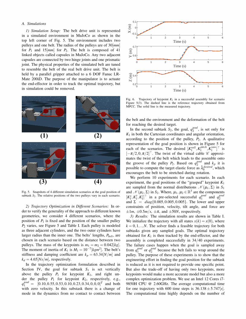
A. Simulations
1) Simulation Setup: The belt drive unit is representedin a simulated environment in MuJoCo as shown in thetop left corner of Fig. 5. The environment includes twopulleys and one belt. The radius of the pulleys are of 30[mm]for P1 and 15[mm] for P2. The belt is composed of 41linked objects called capsules in MuJoCo. Any two adjacentcapsules are connected by two hinge joints and one prismaticjoint. The physical properties of the simulated belt are tunedto resemble the belt of the real belt drive unit. The belt isheld by a parallel gripper attached to a 6 DOF Fanuc LR-Mate 200iD. The purpose of the manipulator is to actuatethe end-effector in order to track the optimal trajectory, butin simulation could be removed.
(1)
(4)(3)
(2)
Fig. 5. Snapshots of 4 different simulation scenarios at the goal position ofsubtask S2. The relative positions of the two pulleys vary in each scenario.
2) Trajectory Optimization in Different Scenarios: In or-der to verify the generality of the approach to different knowngeometries, we consider 4 different scenarios, where theposition of P1 is fixed and the position of the smaller pulleyP2 varies, see Figure 5 and Table I. Each pulley is modeledas three adjacent cylinders, and the two outer cylinders havelarger radius than the inner one. The belts’ lengths, Pbelt , arechosen in each scenario based on the distance between twopulleys. The mass of the keypoints is m1 = m2 = 0.042[kg].The moment of inertia of K1 is M1 = 10−7[kgm2]. The belt’sstiffness and damping coefficient are kp = 63.34[N/m] andkd = 4.65[Ns/m], respectively.
In the trajectory optimization formulation described inSection IV, the goal for subtask S1 is set verticallyabove the pulley P1 for keypoint K1, and right un-der the pulley P1 for keypoint K2, respectively, e.g.,qgoal
1 = [0.10,0.55,0.53,0.10,0.23,0.34,0,0,0]T and bothwith zero velocity. In this substask there is a change ofmode in the dynamics from no contact to contact between
0 1 2 3 4 5 6
Time (s)
-0.1
0
0.1
X (
m)
0 1 2 3 4 5 6
Time (s)
0.6
0.7
Y (
m)
0 1 2 3 4 5 6
Time (s)
0.2
0.4
Z (
m)
Fig. 6. Trajectory of keypoint K1 in a successful assembly for scenarioFigure 5(3). The dashed line is the reference trajectory obtained fromMPCC. The solid line is the measured trajectory.
the belt and the environment and the deformation of the beltfor reaching the desired target.
In the second subtask S2, the goal, qgoal2 , is set only for
K1 in both the Cartesian coordinates and angular orientation,according to the position of the pulley, P2. A qualitativerepresentation of the goal position is shown in Figure 5 foreach of the scenarios. The desired [Kroll
1 ,K pitch1 ,Kyaw
1 ]> is[−π/2,0,π/2]>. The twist of the virtual cable C approxi-mates the twist of the belt which leads to the assemble ontothe groove of the pulley P2. Based on qgoal
2 and kp it ispossible to compute the target elastic force as λ desired
0 , whichencourages the belt to be stretched during rotation.
We perform 10 experiments for each scenario. In eachexperiment, the goal positions of the “grasped” keypoint K1are sampled from the normal distributions N (µ1, Σ) in S1and N (µ2, Σ) in S2. Where, µ1, µ2 ∈R3 are the components[Kx
1 ,Ky1 ,K
z1]> in a pre-selected successful qgoal
1 and qgoal2
and Σ = diag{0.005,0.005,0.005}. The lower and upperconstraints of position, velocity, tilt angle, and force are±1m, ±0.5m/s, ±π , and ±50N, respectively.
3) Results: The simulation results are shown in Table I.We initialize the trajectory with all states x(k) = x(0), wherek = 0,1, ..,N. The solver finds a feasible trajectory for bothsubtasks given any sampled goals. The optimal trajectoryobtained for K1 is then tracked by the end-effector, and theassembly is completed successfully in 34/40 experiments.The failure cases happen when the goal is sampled awayfrom qgoal
1 or qgoal2 because the belt fails to wrap around the
pulley. The purpose of these experiments is to show that theengineering effort in finding the goal position for the subtaskis reduced as it is not required to provide one specific point.But also the trade-off of having only two keypoints, morekeypoints would make a more accurate model but also a morecomplex optimization problem. We use an Intel 12 Cores i7-9850H CPU @ 2.60GHz. The average computational timefor one trajectory with 600 time steps is 36.138± 5.747[s].The computational time highly depends on the number of

TABLE ISIMULATION RESULTS IN 4 SCENARIOS. IN EACH SCENARIO THE POSITION OF THE PULLEY CENTER O2 VARIES.
Pbelt O1 (center of P1) O2 (center of P2) Feasible trajectory Successful assemblyScenario 1 0.4m [0.100, 0.550, 0.340] [0.100, 0.680, 0.340] 10/10 10/10Scenario 2 0.4m [0.100, 0.550, 0.340] [0.100, 0.642, 0.432] 10/10 8/10Scenario 3 0.4m [0.100, 0.550, 0.340] [0.100, 0.645, 0.275] 10/10 7/10Scenario 4 0.6m [0.100, 0.550, 0.340] [0.100, 0.780, 0.340] 10/10 9/10
XYZ
(a) (b) (c)
(d)(e)(f)
Fig. 7. Snapshots of the experiment.
0 5 10 15 20 25 30
Time (s)
-40
-20
0
20
Forc
es (
N)
Forces vs Time
YZX
0 5 10 15 20 25 30
Time (s)
-0.05
0
0.05
0.1
Posi
tions
(m
)
Positions vs Time
YZX
Fig. 8. Forces and positions of the end-effector in a successful experiment.The red circle and square represent the end of subtask S1, S2, respectively.
time steps selected. Figure 6 shows one full successfulassembly trajectory for scenario Figure 5(3).
B. Real-World Experiments
1) Experimental Setup: As shown in Figure 1, the ex-periment environment includes a 6 DOF FANUC LR-Mate200iD, an ATI Mini45 F/T sensor, and a 3D printed beltdrive unit of the same dimensions in the assembly challenge[6] fixed on a vise. The belt is the same as in the challengewith length 0.40[m] and is gripped by a parallel jaw gripper.We assume no slip between the belt and the robot gripper.The pose of the pulleys is known exactly.
2) Results: Figure 7 provides the snapshots of the mainphases during the execution of a successful experiment. Fig-ure 8 shows the trajectory of the gripper tip that correspondsto K1 and the measured forces at the robot’s wrist along the
trajectory. In the beginning, (Figure 7a), the belt approachesthe pulley and position X increases and the forces are zero.The position Z goes down at 5.57[s] to avoid the outercylinder of the first pulley. At 6.29[s], position X stopsincreasing because the pulley is reached (Figure 7b). Thenthe Z position increases as the belt is lifted and contacts thepulley at 7.82[s] with a corresponding increase in force alongthe negative direction in Z. At 10.50[s], the system accom-plishes S1 (Figure 7c). After that, the belt is rotated aroundO1 (the Z position decreases, and Y position increases) whilebeing stretched (Figure 7d). In this phase, the measured netforce is closed to the desired elastic force λ desired
0 . The targetorientations are [Kroll
1 ,K pitch1 ,Kyaw
1 ]> = [−π/2,0,π/4]>. Thebelt is twisted so that it hooks the second pulley withoutjamming. Finally, the goal of subtask S2 is reached at 29.00[s](Figure 7e) and the gripper releases the belt (Figure 7f).
The experiment has been repeated multiple times but giventhe robot’s accuracy the results were similar to each other.
VI. CONCLUSION
In this paper, we propose a trajectory optimization for-mulation to assemble the belt drive unit. We propose a 3Dkeypoints representation to model the elastic belt, whichsimplifies the complexity of the trajectory optimization prob-lem. The problem is formulated as an MPCC with comple-mentarity constraints to model the hybrid dynamics due tocontact and elastic forces. Simulations results show that theproposed approach can find feasible trajectories for the beltdrive unit assembly with known but variable geometry. To thebest of our knowledge, this is the first work that formalizesthe trajectory optimization problem for the belt drive unitassembly, and the solution works in the real system. Severalfuture works are possible. The current method is based onthe execution of an open-loop trajectory which could failunder uncertainties in the position of the pulleys or of thebelt. Adding a feedback controller is fundamental for amore robust and reliable solution. Moreover, in order toimprove the generality of the problem, we are interested inan autonomous selection of the 3D keypoints for a giventask. Our formulation of a trajectory optimization problemfor deformable objects using complementarity constraints isnot limited to belt drive unit assembly. The proposed methodmight be applied to a wider range of tasks such as cablerouting and wire harness.

REFERENCES
[1] Y. LeCun, Y. Bengio, and G. Hinton, “Deep learning,” nature, vol.521, no. 7553, pp. 436–444, 2015.
[2] A. Krizhevsky, I. Sutskever, and G. E. Hinton, “Imagenet classificationwith deep convolutional neural networks,” Communications of theACM, vol. 60, no. 6, pp. 84–90, 2017.
[3] D. Silver, J. Schrittwieser, K. Simonyan, I. Antonoglou, A. Huang,A. Guez, T. Hubert, L. Baker, M. Lai, A. Bolton et al., “Masteringthe game of go without human knowledge,” nature, vol. 550, no. 7676,pp. 354–359, 2017.
[4] S. Jin, X. Zhu, C. Wang, and M. Tomizuka, “Contact pose identifi-cation for peg-in-hole assembly under uncertainties,” arXiv preprintarXiv:2101.12467, 2021.
[5] M. T. Mason, “Toward robotic manipulation,” Annual Review ofControl, Robotics, and Autonomous Systems, vol. 1, pp. 1–28, 2018.
[6] F. von Drigalski, C. Schlette, M. Rudorfer, N. Correll, J. Triyonoputro,W. Wan, T. Tsuji, and T. Watanabe, “Robots assembling machines:Learning from the world robot summit 2018 assembly challenge,”2019.
[7] Y. F. Zheng, R. Pei, and C. Chen, “Strategies for automatic assemblyof deformable objects,” in Proceedings. 1991 IEEE InternationalConference on Robotics and Automation, 1991, pp. 2598–2603 vol.3.
[8] I. G. Ramirez-Alpizar, K. Harada, and E. Yoshida, “Motion planningfor dual-arm assembly of ring-shaped elastic objects,” in 2014 IEEE-RAS International Conference on Humanoid Robots, 2014, pp. 594–600.
[9] J. Zhu, B. Navarro, R. Passama, P. Fraisse, A. Crosnier, and A. Cheru-bini, “Robotic manipulation planning for shaping deformable linearobjects with environmental contacts,” IEEE Robotics and AutomationLetters, vol. 5, no. 1, pp. 16–23, 2020.
[10] K. Tatemura and H. Dobashi, “Strategy for roller chain assembly withparallel jaw gripper,” IEEE Robotics and Automation Letters, vol. 5,no. 2, pp. 2435–2442, 2020.
[11] T. Tang, C. Wang, and M. Tomizuka, “A framework for manipulatingdeformable linear objects by coherent point drift,” IEEE Robotics andAutomation Letters, vol. 3, no. 4, pp. 3426–3433, 2018.
[12] S. Jin, C. Wang, X. Zhu, T. Tang, and M. Tomizuka, “Real-timestate estimation of deformable objects with dynamical simulation,”in Workshop on Robotic Manipulation of Deformable Objects 2020IEEE/RSJ International Conference on Intelligent Robots and Systems(IROS), 2020.
[13] M. Posa, C. Cantu, and R. Tedrake, “A direct method for trajectory op-timization of rigid bodies through contact,” The International Journalof Robotics Research, vol. 33, no. 1, pp. 69–81, 2014.
[14] P. Kolaric, D. Jha, A. Raghunathan, F. Lewis, M. Benosman,D. Romeres, and D. Nikovski, “Local policy optimization fortrajectory-centric reinforcement learning,” in IEEE International Con-ference on Robotics and Automation (ICRA). IEEE, 2020, pp. 5094–5100.
[15] K. Yunt and C. Glocker, “Trajectory optimization of mechanical hybridsystems using sumt,” in 9th IEEE International Workshop on AdvancedMotion Control, 2006. IEEE, 2006, pp. 665–671.
[16] R. Goebel, R. G. Sanfelice, and A. R. Teel, “Hybrid dynamicalsystems,” IEEE Control Systems Magazine, vol. 29, no. 2, pp. 28–93, 2009.
[17] R. Fierro, A. K. Das, V. Kumar, and J. P. Ostrowski, “Hybrid control offormations of robots,” in Proceedings 2001 ICRA. IEEE InternationalConference on Robotics and Automation (Cat. No.01CH37164), vol. 1,2001, pp. 157–162 vol.1.
[18] L. P. Kaelbling and T. Lozano-Perez, “Hierarchical task and motionplanning in the now,” in 2011 IEEE International Conference onRobotics and Automation, 2011, pp. 1470–1477.
[19] K. Yunt and C. Glocker, “A combined continuation and penalty methodfor the determination of optimal hybrid mechanical trajectories,” inIUTAM Symposium on Dynamics and Control of Nonlinear Systemswith Uncertainty. Springer, 2007, pp. 187–196.
[20] K. Yunt, “An augmented lagrangian based shooting method for theoptimal trajectory generation of switching lagrangian systems,” Dy-namics of Continuous, Discrete and Impulsive Systems Series B:Applications and Algorithms, vol. 18, no. 5, pp. 615–645, 2011.
[21] Z.-Q. Luo, J.-S. Pang, and D. Ralph, Mathematical programs withequilibrium constraints. Cambridge University Press, 2008.
[22] F. Lamiraux and L. E. Kavraki, “Planning paths for elastic objectsunder manipulation constraints,” The International Journal of RoboticsResearch, vol. 20, no. 3, pp. 188–208, 2001.
[23] M. Moll and L. E. Kavraki, “Path planning for deformable linearobjects,” IEEE Transactions on Robotics, vol. 22, no. 4, pp. 625–636,2006.
[24] D. Navarro-Alarcon, Y. Liu, J. G. Romero, and P. Li, “Model-free visually servoed deformation control of elastic objects by robotmanipulators,” IEEE Transactions on Robotics, vol. 29, no. 6, pp.1457–1468, 2013.
[25] J. Zhu, B. Navarro, P. Fraisse, A. Crosnier, and A. Cherubini, “Dual-arm robotic manipulation of flexible cables,” in 2018 IEEE/RSJInternational Conference on Intelligent Robots and Systems (IROS),2018, pp. 479–484.
[26] S. Jin, C. Wang, and M. Tomizuka, “Robust deformation modelapproximation for robotic cable manipulation,” in 2019 IEEE/RSJInternational Conference on Intelligent Robots and Systems (IROS),2019, pp. 6586–6593.
[27] A. Nair, D. Chen, P. Agrawal, P. Isola, P. Abbeel, J. Malik, andS. Levine, “Combining self-supervised learning and imitation forvision-based rope manipulation,” 03 2017.
[28] N. Ratliff, M. Zucker, J. A. Bagnell, and S. Srinivasa, “Chomp:Gradient optimization techniques for efficient motion planning,” in2009 IEEE International Conference on Robotics and Automation,2009, pp. 489–494.
[29] M. Kalakrishnan, S. Chitta, E. Theodorou, P. Pastor, and S. Schaal,“Stomp: Stochastic trajectory optimization for motion planning,” in2011 IEEE International Conference on Robotics and Automation,2011, pp. 4569–4574.
[30] J. Schulman, Y. Duan, J. Ho, A. Lee, I. Awwal, H. Bradlow, J. Pan,S. Patil, K. Goldberg, and P. Abbeel, “Motion planning with sequentialconvex optimization and convex collision checking,” The InternationalJournal of Robotics Research, vol. 33, no. 9, pp. 1251–1270, 2014.
[31] P. Foehn, D. Falanga, N. Kuppuswamy, R. Tedrake, and D. Scara-muzza, “Fast trajectory optimization for agile quadrotor maneuverswith a cable-suspended payload.” RSS, 2017.
[32] L. Manuelli, W. Gao, P. R. Florence, and R. Tedrake, “kpam: Keypointaffordances for category-level robotic manipulation,” 2019.
[33] A. U. Raghunathan and L. T. Biegler, “An interior point method formathematical programs with complementarity constraints (mpccs),”SIAM Journal on Optimization, vol. 15, no. 3, pp. 720–750, 2005.
[34] E. Todorov, T. Erez, and Y. Tassa, “Mujoco: A physics engine formodel-based control,” in 2012 IEEE/RSJ International Conference onIntelligent Robots and Systems, 2012, pp. 5026–5033.
[35] A. Wachter and L. T. Biegler, “On the implementation of an interior-point filter line-search algorithm for large-scale nonlinear program-ming,” Math. Program., vol. 106, no. 1, p. 25–57, Mar. 2006.


![Fakulta elektrotechnick a Czech Technical University in Prague Faculty … · 2017. 4. 15. · interactive 2D shape manipulation [IMH05], deformable image registra-tion [SDC09a],](https://static.fdocuments.net/doc/165x107/60c1036ee2c3862893661187/fakulta-elektrotechnick-a-czech-technical-university-in-prague-faculty-2017-4.jpg)


