Train Scheduling and Rescheduling in the UK witha Modified Shifting Bottleneck Procedure∗

Banafsheh Khosravi1, Julia A. Bennell1, and Chris N. Potts2

1 School of Management, CORMSIS Research Group, University ofSouthamptonSouthampton, SO17 1BJ, UKB.Khosravi@soton.ac.uk, J.A.Bennell@soton.ac.uk

2 School of Mathematics, CORMSIS Research Group, University ofSouthamptonSouthampton, SO17 1BJ, UKC.N.Potts@soton.ac.uk

AbstractThis paper introduces a modified shifting bottleneck approach to solve train scheduling andrescheduling problems. The problem is formulated as a job shop scheduling model and a mixedinteger linear programming model is also presented. The shifting bottleneck procedure is a well-established heuristic method for obtaining solutions to the job shop and other machine schedulingproblems. We modify the classical shifting bottleneck approach to make it suitable for the typesof job shop problem that arises in train scheduling. The method decomposes the problem intoseveral single machine problems. Different variations of the method are considered with regard tosolving the single machine problems. We compare and report the performance of the algorithmsfor a case study based on part of the UK railway network.

1998 ACM Subject Classification G.1.6 Optimization, Integer programming

Keywords and phrases Train Scheduling and Rescheduling, Job Shop Scheduling, Shifting Bot-tleneck Procedure

Digital Object Identifier 10.4230/OASIcs.ATMOS.2012.120

1 Introduction

Meeting the ever-increasing demand for additional rail capacity is a key issue for many traincompanies. There are two ways of providing the additional capacity for passengers andfreight users. One way is to construct new sections of track and another is through therelease of capacity on the current rail network. Whereas first option is very costly, the latteris linked to train scheduling which reduces the loss of capacity of the network through betterscheduling decisions. The applications of operational research methodologies in combinationwith advances in technology can provide great incentives for the rail industry.

After the pioneering publication of Szpigel [17], formulating the train scheduling problemas a job shop scheduling problem offered a promising new research direction. However,there have been several job shop scheduling approaches such as mathematical programmingtechniques by Szpigel [17] and Sahin [16], constraint programming approaches by Oliveiraand Smith [12] and Rodriguez [14], and the alternative graph formulation by D’Ariano et

∗ This work was partially funded and supported by School of Management, former LASS Faculty of theUniversity of Southampton and the LANCS Initiative.

© Banafsheh Khosravi, Julia A. Bennell, and Chris N. Potts;licensed under Creative Commons License ND

12th Workshop on Algorithmic Approaches for Transportation Modelling, Optimization, and Systems (ATMOS’12).Editors: Daniel Delling, Leo Liberti; pp. 120–131

OpenAccess Series in InformaticsSchloss Dagstuhl – Leibniz-Zentrum für Informatik, Dagstuhl Publishing, Germany

B. Khosravi, J.A. Bennell, and C.N. Potts 121

al. [6], Corman et al. [5] and Liu and Kozan [9]. There are two main lines of research withregard to the complexity of the railway infrastructure. In the first category, Szpigel [17],Sahin [16] and Oliveira and Smith [12] each address a single line railway with single andmultiple track segments. More realistic networks are considered in the second category ofstudies. Rodriguez [14] schedules trains in a terminal station, whereas D’Ariano et al. [6]and Corman et al. [5] provide solutions for a dispatching area of a railway network withpassengers and freight. Further, Liu and Kozan [9] investigate a case study of a railwaynetwork for the transport of coal.

A decomposition of the railway planning process into strategic, tactical and operationallevels is proposed by Huisman et al. [8], Caprara et al. [4] and Lusby et al. [10] as dealingwith the whole problem is hard and complicated. Train scheduling and rescheduling are thesubtasks of the planning process in tactical and operational levels, respectively. For a generaloverview of operations research models and methods in railway transportation, see Huismanet al. [8], Caprara et al. [4], Lusby et al. [10] and Cacchiani and Toth [2].

This paper aims to refine existing models for train scheduling and rescheduling problemswith the goal of obtaining a more generic model that includes important additional constraints.The model is customised to the UK railway network and is evaluated through a case study.The train scheduling and rescheduling problems are addressed in Section 2. Section 3 containsthe development of our proposed model. In Section 4, we adapt the shifting bottlenecksolution approach for the particular job shop problems that arise in train scheduling. Theperformance of the proposed methods on a real-world case study based on London and SouthEast area of the UK that is a dense and complex network of interconnected lines is reportedin Section 5. Finally, Section 6 presents some conclusions and suggestions for future work.

2 Problem definition

Depending on the level of detail about track topology and train dynamics, the train schedulingand rescheduling problems can be classified as microscopic or macroscopic problems [3]. Thispaper investigates the train scheduling and rescheduling problems at the micro level includingdetailed information about the tracks and train movements. Our experimental evaluation isbased on a bottleneck area in the South East of the UK where the network has a complicatedstructure including several junctions and stations.

The movement of a train on the network is controlled for safety reasons by signalswhich divide the network to track sections called blocks. Given predetermined routes from agiven origin to a given destination, a schedule determines starting times of trains enteringeach block and the order of trains on each block. Each train needs a minimum specifiedrunning time to travel on a block. If there is a scheduled stop at a station, the train needs aminimum dwell time for the passengers or freight to board/load and alight/unload. Also,safety considerations impose a headway, which is the minimum time between two consecutivetrains travelling on the same block. Various signalling systems are used in different countries.In this study, we consider four-aspect signalling which is common for the main lines of theUK network, as shown in Figure 1: red for stop (danger), yellow for approach (caution),double yellow for advance approach (preliminary caution) and green for clear. Each aspectgives information for 4 blocks ahead, thus enabling the train driver to adjust the speedand to keep sufficient separation between trains to allow safe braking. According to thesafety principles, only one train can travel on a block at a time and a conflict occurs whenmore than one train is assigned to a block. Another issue is the deadlock that arises whencertain trains are currently positioned in a way that none can move further without causing

ATMOS’12

122 Train Scheduling and Rescheduling in the UK

Block section

T1 T2

Green Double Yellow Yellow Red

Figure 1 4-aspect signalling system.

a collision. A deadlock happens usually in complicated networks with bidirectional travels.Thus, being conflict-free and deadlock-free are essential characteristics of a feasible schedule.The above-mentioned operational and safety issues are treated as constraints in our problem.

It is also important to take into account the possibility of delay propagation in a railwaynetwork which is due to the high interdependency of the trains. Thus, the objective of ourproblem is to minimize delay propagation. In summary, the aim of train scheduling is tomake the best usage of the existing capacity by allocating trains to blocks. In this study,timetable components including scheduled running time, dwell time and headway and theirbuffer times or margins are assumed to be fixed and we try to minimize the delay by selectingefficient timings and ordering of trains on blocks. Train scheduling can be performed at atactical level, which can take up to a year. When trains are operated according to a plan,disruptions can cause deviations to that plan due to various causes such as train delays,accidents, track maintenance, no-shows for crew, weather conditions, etc. Train reschedulingresponds to disruptions in an operational level, where a new schedule is required in a matterof minutes or seconds. The same scheduling technique can be implemented for real-timetraffic management if the solution method is fast enough.

3 Problem formulation

In this study, we make use of the similarity between train scheduling problem and thewell-known job shop scheduling problem. Job shop scheduling assigns jobs to machines in away that a machine can process only one job at a time. Likewise, a block can be occupiedby only one train at a time according to the line blocking which is a safety principle fortrain movement. Thus, a train traversing a block is analogous to a job being processed on amachine, and is referred to as an operation.

The following notation is used for parameters and decision variables in the mathematicalprogramming formulation for the train scheduling problem.

I: set of jobs/trainsi,j: indices for jobs (i = 1, . . . , I and j = 1, . . . , I)ri: non-negative release time of job i/scheduled departure time of train i

from its origindi: non-negative due date of job i/scheduled arrival time of train i at its

destinationwi: non-negative importance weight of job i/train i

(mi1, . . . , mi,li ): sequence of machines to be visited by job i/sequence of blocks to betraversed by train i

(i, m): job, machine indices/train, block indices, for m = mi1, . . . , mi,li

O: set of operations defined by indices (i, m), for i ∈ I, m = mi1, . . . , mi,li

B. Khosravi, J.A. Bennell, and C.N. Potts 123

pim: operation time for job i on machine m/running time for train i onblock m

si(m): the index of its immediate successor operation (index of its third suc-cessor operation) for two-aspect signalling (four-aspect signalling) of(i, m)

Si(m): a set containing index (i, m) for two-aspect signalling, and additionallycontaining the indices of its immediate and second successor operationfor four-aspect signalling

hijm: required time delay (headway) between the start of operations (i, m)and (j, m) when job i precedes job j on machine m

xijm:

{1, if job i precedes job j on machine m

0, otherwisetim: starting time of job i on machine m

Ti: tardiness of job i

To minimize delay propagation of trains with different priorities, the objective is tominimize total weighted tardiness. The tardiness of a job is calculated from the due dateof the job, which is equivalent to the pre-defined time that a train should reach its finaldestination and therefore leave the network. The release time of a job is similarly definedas the pre-defined time that the train should leave its origin and thus enter the network.Weights can be determined from train priorities. Thus, the train scheduling problem can beformulated as a job shop scheduling problem with additional constraints, and a correspondingmixed integer linear programming (MILP) model is specified below.

Minimize z =∑i∈I

wiTi (1)

subject toTi ≥ ti,mi,li

+ pi,mi,li− di i ∈ I (2)

ti,mi,1 ≥ ri i ∈ I (3)ti,mk

− ti,mk−1 ≥ pi,mk−1 i ∈ I, k = 2, . . . , li (4)tjm − tim + B(1− xijm) ≥ max{pim, hijm} (i, m), (j, m) ∈ O (5)tim − tjm + B(1− xjim) ≥ max{pjm, hjim} (i, m), (j, m) ∈ O (6)

tjm − tisi(m) + B(1− xijm) ≥∑

(i,k)∈Si(m)

pik (i, m), (j, m) ∈ O (7)

tim − tjsj(m) + B(1− xjim) ≥∑

(j,k)∈Sj(m)

pjk (i, m), (j, m) ∈ O (8)

xijm + xjim = 1 (i, m), (j, m) ∈ O (9)xijm ∈ {0, 1} (i, m), (j, m) ∈ O (10)

In this formulation, the total weighted tardiness objective function is defined in (1). Thetardiness of a job is defined in (2) by considering its starting time on the last machine of itssequence, its processing time on that machine and the due date of the job; this is equivalentto defining a train’s delay. Ensuring that the starting time of a job on the first machine of itssequence is no earlier than its release time is achieved through (3), which means a train canstart only after it is ready on the first block. Constraints (4) are called the set of conjunctive

ATMOS’12

124 Train Scheduling and Rescheduling in the UK

constraints to ensure the processing order of a job on consecutive machines. It determinesthe running and dwell time constraints for trains. Modified disjunctive constraints (5) and(6) specify the ordering of different jobs on the same machine, and they are adapted to definethe minimum headway between consecutive trains. Alternative constraints (7) and (8) forcea job to remain on a machine after completing its process until the next machine becomesavailable. This pair of constraints can represent the signalling system of the network.

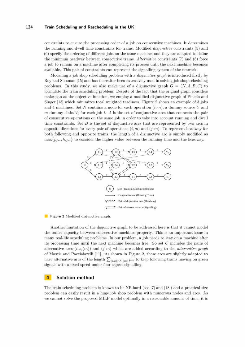
Modelling a job shop scheduling problem with a disjunctive graph is introduced firstly byRoy and Sussman [15] and has thereafter been extensively used in solving job shop schedulingproblems. In this study, we also make use of a disjunctive graph G = (N, A, B, C) toformulate the train scheduling problem. Despite of the fact that the original graph considersmakespan as the objective function, we employ a modified disjunctive graph of Pinedo andSinger [13] which minimizes total weighted tardiness. Figure 2 shows an example of 3 jobsand 4 machines. Set N contains a node for each operation (i, m), a dummy source U andm dummy sinks Vi for each job i. A is the set of conjunctive arcs that connects the pairof consecutive operations on the same job in order to take into account running and dwelltime constraints. Set B is the set of disjunctive arcs that are represented by two arcs inopposite directions for every pair of operations (i, m) and (j, m). To represent headway forboth following and opposite trains, the length of a disjunctive arc is simply modified asmax{pjm, hijm} to consider the higher value between the running time and the headway.

2, 4

1, 2 1, 3

U

1, 4

2, 1

1, 1

5

2, 2 2, 3

3, 3 3, 2 3, 1 3, 4

V 1

V 2

V 3

i, j : Job (Train) i, Machine (Block) n

: Conjunctive arc (Running Time)

: Pair of disjunctive arcs (Headway)

: Pair of alternative arcs (Signalling)

0

5 1 4 8

2 6 5

0

5

4

3 7 9

Figure 2 Modified disjunctive graph.

Another limitation of the disjunctive graph to be addressed here is that it cannot modelthe buffer capacity between consecutive machines properly. This is an important issue inmany real-life scheduling problems. In our problem, a job needs to stay on a machine afterits processing time until the next machine becomes free. So set C includes the pairs ofalternative arcs (i, si(m)) and (j, m) which are added according to the alternative graphof Mascis and Pacciaiarelli [11]. As shown in Figure 2, these arcs are slightly adapted tohave alternative arcs of the length

∑(i,k)∈Si(m) pik to keep following trains moving on green

signals with a fixed speed under four-aspect signalling.

4 Solution method

The train scheduling problem is known to be NP-hard (see [7] and [18]) and a practical sizeproblem can easily result in a huge job shop problem with numerous nodes and arcs. Aswe cannot solve the proposed MILP model optimally in a reasonable amount of time, it is

B. Khosravi, J.A. Bennell, and C.N. Potts 125

preferable to employ local search methods for which computational time is more predictable.The shifting bottleneck (SB) procedure of Adams et al. [1] is a well-known heuristic for

solving a classical job shop scheduling problem that is formulated as a disjunctive graph.The success in applying the SB procedure on benchmark instances in job shop schedulingliterature has led to a number of studies that employ the SB approach. It can be also usedas a framework for other heuristics such as tabu search, simulated annealing and geneticalgorithms. Although there is no theoretical performance guarantee for SB, its empiricalperformance has a good track record.

The SB procedure is a deterministic decomposition approach to solve multiple machineproblems by selecting each machine in turn and using the solution of the single machineproblem to define the processing order of jobs on that machine. According to Pinedo andSinger [13], the solution method includes three main steps of sub-problem formulation,sub-problem optimization and bottleneck selection (Figure 3). To find a feasible solution, weneed an acyclic order of operations by selecting exactly one arc of each pair of disjunctiveand alternative arcs. Mascis and Pacciarelli [11] provide some key properties and feasibilityanalysis of a blocking job shop problem. In this paper, a modified SB procedure is proposedfor the train scheduling and rescheduling problems. It is inspired by Pinedo and Singer [13]but modified for train scheduling to include additional constraints.

Yes

No

Sub-problem

Formulation

Sub-problem

Optimization

All Machines

Scheduled?

Bottleneck

Selection Start End

Figure 3 Shifting Bottleneck (SB) flowchart, adapted from Pinedo and Singer [13].

In general, the proposed SB differs from the conventional SB in solving the single machineproblem and finding the bottleneck. While the original SB considers an exact method tosolve the single machine problem of minimizing the maximum lateness of jobs having releasedates on a single machine (problem 1|rj |Lmax), the new SB employs a heuristic to solve thesingle machine problem of minimizing the total weighted tardiness of jobs having releasedates on a single machine (problem 1|rj |

∑wjTj). Bottleneck selection is based on maximum

lateness calculations in original SB, whereas the proposed SB makes use of total weightedtardiness evaluations. The proposed SB procedure uses the following notation.

j, k: job indices(j, m) job, machine indices for the operation that processes job j on machine

m

rjm: local release date for operation (j, m)pjm: processing time of operation (j, m) of job j

dkjm: local due date of operation (j, m) with respect to the due date of job k

L((j, m), Vk): the longest path from operation (j, m) to Vk, the sink corresponding tojob k

Cjm: completion time of job j on machine m

Ck: completion time of job k

T kjm: tardiness of operation (j, m) with respect to the due date of job k

In the following, we introduce three main steps of the new SB algorithm. In the first

ATMOS’12

126 Train Scheduling and Rescheduling in the UK

algorithm, we develop a heuristic based on a well-known priority rule for 1|rj |∑

wjTj whichis called the apparent tardiness cost (ATC) rule. The ATC is a dynamic rule that calculatesa ranking index for each job to be sequenced next on a machine. Under this rule, the highestranking job is selected among the remaining jobs to be processed next. Here, the singlemachine heuristic embeds an adaptation of the ATC rule developed by Pinedo and Singer [13].Because of the ATC index, we refer to our first SB algorithm as SB-ATC.

SB-ATC algorithmGenerate an instance of 1|rj |

∑wjTj and for each operation calculate

rjm = L(U, (j, m)), (11)

dkjm =

{max{Ck, dk} − L((j, m), Vk) + pjm if L((j, m), Vk) exists,∞ otherwise.

(12)

Select the operation (j, m) with the highest index

Ijm(t) =n∑

k=1

wk

pjm

(−

(dkjm − pjm + (rjm − t))+

Kp̄

), (13)

where t is the time that the machine becomes available, p̄ is the average processing time ofjobs assigned to machine m, and K is a scaling parameter whose value can be determinedthrough computational tests.Choose a machine m with its corresponding sequence of operations that minimizes

n∑k=1

wk

(max

(j,m)∈Nm

T kjm

), T k

jm = max{Cjm − dkjm, 0}. (14)

where Nm is the set of nodes corresponding to the operations processed on machine m.

The second SB algorithm is based on an active schedule generation (ASG) heuristic tosolve the single machine problems. The so-called SB-ASG selects the job with the smallestrelease date among potential candidates with rjm < ECT, where ECT is the smallest possiblecompletion time of the job to be scheduled next. The third SB algorithm is developed onthe basis of the Schrage scheduling heuristic and is therefore named SB-SCH. In SB-SCH,among potential candidates with rjm ≤ EST, where EST is the smallest possible startingtime of the job to be scheduled next, it selects the job with d∗jm = minkdk

jm.Within the SB solution process, arcs are added gradually to the problem through sub-

problem optimization step. We need to ensure that the disjunctive and alternative arcs to beadded do not lead to infeasible solutions. Assume that machine m is selected in the bottleneckselection step. All jobs on that machine are sequenced by using one of the mentioned singlemachine heuristics. The disjunctive arcs can be added based on the sequence of the jobson machine m. Consequently, we add an alternative arc from (i, si(m)) to (j, m) if there isa disjunctive arc from (i, m) to (j, m). The next step is to use the static implication rulesof D’Ariano et al. [6] to add implied alternative arcs for the following trains running oncommon blocks. Further, we fix the implied arcs among the jobs on a machine for all trainson common blocks. Through this process, the main characteristics of a timetable to beconflict-free and deadlock-free are guaranteed.

B. Khosravi, J.A. Bennell, and C.N. Potts 127

A First Come First Served (FCFS) algorithm is also implemented, which is a simpledispatching rule. It is close to the dispatcher’s behaviour in a real-time decision-makingenvironment. Our proposed SB algorithms are tested against FCFS in terms of the solutionquality.

5 Computational results

In this section, we discuss a real-world implementation of the proposed SB algorithms. Theexperiments are based on the London Bridge area in the South East of the UK, chosenbecause it is a dense and complicated network of interconnected lines for passengers in andout of London, East Sussex and the Channel Tunnel. Figure 4 shows the configuration ofthe network. It is a critical corridor with known capacity and performance issues, whichare made more complex by the addition of a new high speed line. The partial network weconsider is about 15 km long including busy stations like London Charing Cross, LondonWaterloo, London Cannon Street, New Cross and Deptford, and a total of 28 platforms.The network includes 135 blocks with unidirectional and bidirectional traffic. Passengertrains start their journey from either Charing Cross or Cannon street and travel through 75blocks in order to leave the network, or they enter the network and travel through 76 blocksterminating at one of the mentioned stations.

Charing Cross

D

C

A

B

Waterloo East

London Bridge

Cannon Street

Metropolitan Junction

Borough Market

Junction

New Cross

Deptford North Kent East

Junction

Blue Anchor

Junction

Spa Road

Junction

6

5

4

3

2

1

1

2

3

4

5

6

A

B

C

D

1 2 3 4 5 6 7

Figure 4 London Bridge diagram.

Our experimental data focus on the off-peak services because there is an on-going stronggrowth in off-peak period commuters. The timetable cycles every 30 minutes for the passengertrains and includes 27 trains. The train timetables, running times and track diagrams areprovided by the primary train operator for this region of the UK. Using this data we simulatereal-life traffic conditions in one cycle under different types of disruptions in the network byperturbing the known running times on certain blocks. Disruptions are classified into threetypes as follows. A minor disruption is where no individual delay is more than 15 minutes.A general disruption is where multiple services are running with delays between 15 to 30minutes. A major disruption is where the majority of train services are delayed by over 30minutes. All algorithms are developed in MS Visual C++ 2010 and run on a PC with a dualcore, 3.00GHz and 4GB RAM. Computational experiments compare the total delay for theschedule arising from the FCFS dispatching rule and the SB algorithms.

ATMOS’12

128 Train Scheduling and Rescheduling in the UK

In the first set of experiments, we generate 18 problem instances across three types ofdisruptions on single and multiple blocks. Note that we need the running times of at least twoblocks to be perturbed to create a major disruption. Random perturbations are generated onthe most common blocks and/or bidirectional blocks which tend to be the most critical ones.An instance is classified as a minor, general or major disruption based on its FCFS output.If FCFS results in a deadlock, we put the instance in the same class as the most similarinstance, in terms of perturbation, with no deadlock. We denote each type of disruption witha code. M and MM show minor disruptions on a single block and multiple blocks respectively.Similarly, G and GG represent general disruptions on a single block and multiple blocks.Major disruptions on two and multiple blocks are indicated by A and AA.

Table 1 summarizes the results of our first set of experiments comprising a single runfor each of 18 generated instances. In the first and second columns of the table, we definethe disruption type and the instance code. The third, fourth and fifth columns indicatewhich block(s) and train(s) are affected and the size of the perturbation, respectively. Theremaining columns display the results of the FCFS, SB-ATC, SB-ASG and SB-SCH delaysin minutes. The best result(s) for an instance among all algorithms are shown in bold. If weconsider the minimum value among three types of SB algorithms, they clearly outperformFCFS as FCFS ends up with either a worse result or a deadlock in 16 out of 18 instances.SB results are as good as FCFS in G3 and they are slightly worse than FCFS only in MM1.As we expected, FCFS algorithm results in a deadlock in many instances as the network iscomplicated with bidirectional travels. So FCFS schedules trains in a way that they cannotmove further without causing a collision, whereas feasibility is guaranteed by SB algorithmsno matter what type of disruption occurs. There is no special trend among the results ofthree types of SB algorithms and none of them leads to better results for all instances.

As deadlocks arise in many instances solved by FCFS algorithm, we generate many moreinstances and only retain the cases where FCFS does not result in deadlock. Table 2 providesthe results for these new instances and for the no-deadlock instances in Table 1. It alsoprovides the delay for the original timetable where there is no disruption. As before, eachrow shows a single run of the instance and the best result(s) for each instance are displayedin bold. As expected, the minimum delay among all SB algorithms is lower than FCFS in10 out of 13 instances. Only in the second instance of general disruption, SB algorithmsperform as well as FCFS. In the last instance of minor disruption and the first instanceof general disruption, FCFS has slightly better results. Comparing the results of three SBvariants, it appears that SB-SCH is the weakest as it is either as good as or worse than theother SB variants. No strong conclusion can be made about the performance of SB-ATC andSB-ASG. The reason for the varied performance is not clear, but it seems that the searchspace is difficult to navigate and applying different dispatching decisions at certain criticalpoints constrains the search space leading to sometimes better and sometimes worse results.

In general, our experiments show that SB procedure is a promising approach for solvingdisruptions with less delay compared to FCFS and avoids deadlock. However, more detailedanalysis is needed to understand the impact of the dispatch rule. SB also suffers fromlong computational times, that are not practical for real-time decision. For complex casesrun times are up to 26 minutes, whereas FCFS computation time is less than a minute.Computational times for all three versions of SB are similar. However, there is scope fordeveloping a more efficient implementation of SB.

B. Khosravi, J.A. Bennell, and C.N. Potts 129

Table 1 Performance of SB algorithms vs FCFS for 3 types of disruption.

InstanceAffected Affected

IncreaseDelay (mins)

block(s) train(s) FCFS SB-ATC SB-ASG SB-SCH

Minor M1 120 22, 23 5 63.50 52.08 62.50 73.00

disruption on M2 4 4, 6, 18, 20 4 102.33 98.67 87.42 114.08

a single block M3 24 2, 3, 5 5 157.17 136.427 62.50 155.92

Minor MM1 15/24 15, 16/2, 5 4.5/4.5 97.83 120.42 105.58 105.58

disruption on MM2 52/71 10, 24/8, 13 4/4 deadlock 124.58 92.67 92.67multiple blocks MM3 20/58 2, 3/13, 22 4.5/4.5 deadlock 184.42 171.17 171.17

General G1 58 9, 12, 25 5 deadlock 291.67 293.58 230.75disruption on G2 71 11, 13, 14 10 deadlock 170.33 184.50 204.92

a single block G3 132 22, 24, 25 6 124.92 147.83 124.92 124.92

General GG1 20/120 3, 6/23, 25 10/10 315.75 169.33 283.42 283.42

disruption on GG2 15/47 2, 15, 16/1, 4, 7 5/5 190.50 227.42 189.25 189.25multiple blocks GG3 56/120 12, 13, 26/22, 24, 27 10/10 deadlock 321.58 466.25 466.25

Major A1 52/47 8-11, 22-25/1-7 30/30 deadlock 1103.42 1342.17 1621.67

disruption on A2 4/59/ 4-7, 18-21/8-14 30/30 deadlock 3216.08 3919.25 3269.25

two blocks A3 58/94 8-14, 22-27/15-21 30/30 deadlock 5753.58 4477.67 4477.67

AA1

14 2, 3, 16, 17 25

deadlock 2478.25 2657.00 2657.0056 12-14, 26, 27 25

71 8-14 25

120 22-27 25

Major

AA2

4 4-7,18-21 25

deadlock 5472.25 5647.00 5323.67disruption on 15 1-3,15-17 25

multiple blocks 58 8-14,22-27 25

94 15-21 25

AA3

24 1-7 25

deadlock 3504.58 3475.00 3475.0047 1-7 25

94 15-21 25

132 22-27 25

Table 2 Performance of SB algorithms vs FCFS for deadlock-free instances.

Delay (mins)FCFS SB-ATC SB-ASG SB-SCH

Timetable 32.17 27.67 30.92 30.92

Minor disruption

63.50 52.08 62.50 73.00102.33 98.67 87.42 114.08157.17 136.42 155.92 155.9297.83 120.42 105.58 105.58

General disruption

96.00 119.67 99.92 99.92124.92 147.83 124.92 124.92315.75 169.33 283.42 283.42190.50 227.42 189.25 189.25

Major disruption

5977.80 6463.38 5368.97 6161.473557.42 3288.50 3288.00 3289.503527.58 3422.00 3390.83 3390.833504.58 3475.00 3475.00 3475.00

ATMOS’12

130 Train Scheduling and Rescheduling in the UK

6 Conclusions and future work

In this paper, the train scheduling and rescheduling problems are modelled as a job shopscheduling problem with additional constraints. The problem is formulated as a MILP usinga modified disjunctive graph. We describe a new optimization framework based on theSB procedure to solve the problem. Three variants of the SB algorithm are suggested andcompared with the most commonly used FCFS dispatching rule. Our experiments focuson a section of the UK rail network that is dense, complicated and congested. It providesa problem instance that is among the most computationally difficult job shop problemswhere the graph is extremely large. It is clear that simply finding a feasible solution isnontrivial, since the FCFS algorithm frequently results in a deadlock. Hence, the proposedoptimization algorithm, which found feasible solutions to all instances, is very promising tomodel and solve this large and complex problem with all the practical constraints. Furtherresearch to improve the solution time and quality of the algorithm includes investigatingmore efficient heuristics that can be embedded in the current framework and exploitingpotential computational speedups.

Acknowledgements We thank the School of Management, the former LASS Faculty of theUniversity of Southampton and the LANCS Initiative for partially funding and supportingthis project. We are also grateful to Southeastern, the train operating company, for providingdata.

References1 J. Adams, E. Balas, D. Zawack. The shifting bottleneck procedure for job shop scheduling.

Management Science, 34(3):391-401, 1988.2 V. Cacchiani, P. Toth. Nominal and robust train timetabling problems. European Journal

of Operational Research, 219(3):727–737, 2012.3 G. Caimi. Algorithmic decision support for train scheduling in a large and highly utilised

railway network. PhD thesis, Swiss Federal Institute of Technology Zurich, 2009.4 A. Caprara, L. Kroon, M. Monaci, M. Peeters, P. Toth, Passenger Railway Optimization,

in: C. Barnhart, G. Laporte (eds.), Transportation, Handbooks in Operations Researchand Management Science 14, Elsevier, 129–187, 2007.

5 F. Corman, A. D’Ariano, D. Pacciarelli, M. Pranzo. A tabu search algorithm for reroutingtrains during rail operations. Transportation Research Part B, 44(1):175–192, 2010.

6 A. D’Ariano, D. Pacciarelli , M. Pranzo. A branch and bound algorithm for schedulingtrains in a railway network. European Journal of Operational Research, 183(2):643–657,2007.

7 M.R. Garey, D.S. Johnson. Computers and Intractability: A Guide to Theory of NP-Completeness. Freeman, San Franscisco, 1979.

8 D. Huisman, L. Kroon, R. Lentink, M. Vromans. Operations Research in passenger railwaytransportation. Statistica Neerlandica 59(4):467–497, 2005.

9 S.Q. Liu, E. Kozan. Scheduling trains as a blocking parallel-machine shop scheduling prob-lem. Computers and Operations Research 36(10):2840-2852, 2009.

10 R. Lusby, J. Larsen, M. Ehrgott, and D. Ryan. Railway track allocation: models andmethods. OR Spectrum, 33(4):843-883, 2011.

11 A. Mascis, D. Pacciarelli. Job shop scheduling with blocking and no-wait constraints.European Journal of Operational Research 143(3):498-517, 2002.

12 E. Oliveira, B.M. Smith. A job-shop scheduling model for the single-track railway schedulingproblem. Technical Report No. 21, School of Computing, University of Leeds, UK, 2000.

B. Khosravi, J.A. Bennell, and C.N. Potts 131

13 M. Pinedo, M. Singer. A shifting bottleneck heuristic for minimizing the total weightedtardiness in a job shop. Naval Research Logistics 46(1):1–17, 1999.

14 J. Rodriguez. A constraint programming model for real-time trains scheduling at junctions.Transportation Research Part B 41(2):231–245, 2007.

15 B. Roy, R. Sussman. Les problèmes d’ordonnancement avec contraintes disjonctives. Tech-nical Report No. 9, SEMA, Paris, 1964.

16 I. Sahin. Railway traffic control and train scheduling based on inter-train conflict manage-ment. Transportation Research Part B 33(7):511–534, 1999.

17 B. Szpigel. Optimal train scheduling on a single track railway. In M. Ross (Ed.). OperationalResearch ’72, Amsterdam, The Netherlands, 343–352, 1973.

18 J. Ullman. NP-complete scheduling problems. Journal of Computer and System Science,10(3):384–393, 1975.

ATMOS’12