TrainingMulti-Layer

NeuralNetworks- the Back-PropagationMethod

(c) MarcinSydow

Training Multi-Layer Neural Networks

- the Back-Propagation Method

(c) Marcin Sydow

TrainingMulti-Layer

NeuralNetworks- the Back-PropagationMethod

(c) MarcinSydow

Plan

training single neuron with continuous activation function

training 1-layer of continuous neurons

training multi-layer network - back-propagation method

TrainingMulti-Layer

NeuralNetworks- the Back-PropagationMethod

(c) MarcinSydow

Training single neuron with continuous activation function

TrainingMulti-Layer

NeuralNetworks- the Back-PropagationMethod

(c) MarcinSydow

Reminder: neuron with continuous activation

function

sigmoid unipolar activation function:

f (net) =1

1 + e−net

sigmoid bipolar activation function:

f (net) =2

1 + e−net− 1

where:

net = wT x

TrainingMulti-Layer

NeuralNetworks- the Back-PropagationMethod

(c) MarcinSydow

Error of continuous neuron

Let's de�ne the following error measure for a single neuron:

E =1

2(d − y)2 =

1

2(d − f (wT x))2

where:

d - desired output (continuous)

y - actual output (continuous) (y = f(net))

(coe�cient 1/2 is selected for simpli�cation of subsequent

computations)

TrainingMulti-Layer

NeuralNetworks- the Back-PropagationMethod

(c) MarcinSydow

Training goal: minimisation of the error

We wish to modify the weight vector w so that the error E is

minimised.

Gradient Method: the direction of maximum descent of the

function (towards the minimum) is opposite to the gradient

vector (of partial derivatives of the error as the function of

weight vector)

∇E (w) =∂E

∂w

∇E (w) = −(d − y)f ′(net)(∂net

∂w1

, . . . ,∂net

∂wp)T =

= −(d − y)f ′(net)x

TrainingMulti-Layer

NeuralNetworks- the Back-PropagationMethod

(c) MarcinSydow

Derivatives of sigmoid functions

Let's observe that:

for unipolar sigmoid function:

f ′(net) = f (net)(f (net)− 1) = y(y − 1)

for bipolar sigmoid function:

f ′(net) =1

2(1− f 2(net)) =

1

2(1− y2)

Thus, the derivative of f can be easily expressed in terms of

itself.

(Now, we can understand why such particular form of activation

function was selected)

TrainingMulti-Layer

NeuralNetworks- the Back-PropagationMethod

(c) MarcinSydow

Learning rule for a continuous neuron

To sum up, the weights of a continuous neuron are modi�ed as

follows:

unipolar:

wnew = wold + η(d − y)y(1− y)x

bipolar:

wnew = wold +1

2η(d − y)(1− y2)x

where: η is the learning rate coe�cient

Notice a remarkable analogy to the delta rule for discrete

perceptron

TrainingMulti-Layer

NeuralNetworks- the Back-PropagationMethod

(c) MarcinSydow

Training 1-layer of neurons with continuous activation function

TrainingMulti-Layer

NeuralNetworks- the Back-PropagationMethod

(c) MarcinSydow

1-layer of neurons with continuous activation

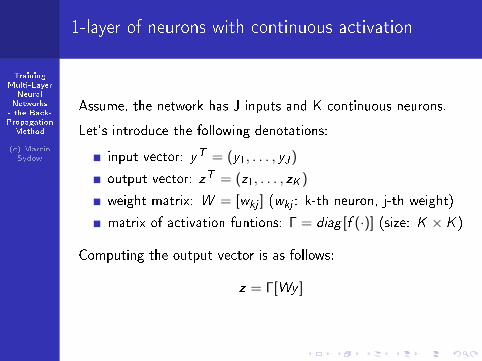
Assume, the network has J inputs and K continuous neurons.

Let's introduce the following denotations:

input vector: yT = (y1, . . . , yJ)

output vector: zT = (z1, . . . , zK )

weight matrix: W = [wkj ] (wkj : k-th neuron, j-th weight)

matrix of activation funtions: Γ = diag [f (·)] (size: K × K )

Computing the output vector is as follows:

z = Γ[Wy ]

TrainingMulti-Layer

NeuralNetworks- the Back-PropagationMethod

(c) MarcinSydow

Training 1-layer of neurons with continuous

activation funtions

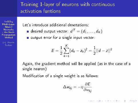
Let's introduce additional denotations:

desired output vector: dT = (d1, . . . , dK )

output error for a single input vector:

E =1

2

K∑k=1

(dk − zk)2 =1

2||d − z ||2

Again, the gradient method will be applied (as in the case of a

single neuron)

Modi�cation of a single weight is as follows:

∆wkj = −η ∂E∂wkj

TrainingMulti-Layer

NeuralNetworks- the Back-PropagationMethod

(c) MarcinSydow

Training 1-layer NN, cont.

Thus, we obtain:

∂E

∂wkj

=∂E

∂netk

∂netk∂wkj

error signal delta of the k-th neuron of the last layer:

δzk = − ∂E

∂netk= (dk − zk)zk(1− zk)

δzk = − ∂E

∂netk=

1

2(dk − zk)(1− zk)2

Notice that: ∂netk∂wkj

= yj

We get the following matrix weight modi�cation formula:

Wnew = Wold + ηδzyT

TrainingMulti-Layer

NeuralNetworks- the Back-PropagationMethod

(c) MarcinSydow

Algorithm for training 1-layer NN

select η, Emax , initialise random weights W , E = 0

for each case from the training set:

compute the output z

mo�fy the weight of the k-th neuron (unipolar/bipolar):

wk ← wk + η(dk − zk)zk(1− zk)y

wk ← wk +1

2η(dk − zk)(1− z2k )y

accumulate the error:

E ← E +1

2

K∑k=1

(dk − zk)2

if all training cases where considered and E < Emax then

complete the training phase. Else, reset the error E and

repeat training on the whole training set.

TrainingMulti-Layer

NeuralNetworks- the Back-PropagationMethod

(c) MarcinSydow

Training multi-layer network - Back-propagation method

TrainingMulti-Layer

NeuralNetworks- the Back-PropagationMethod

(c) MarcinSydow

Multi-layer network

1-layer NN can split the input space into linearly separable

regions.

Each next layer can further transform the space.

As the result, multi-layer network is a universal tool that

theoretically can arbitrarily well approximate any transformation

of the input space into output space.

TrainingMulti-Layer

NeuralNetworks- the Back-PropagationMethod

(c) MarcinSydow

Training of a multi-layer network

We will illustrate training of a multi-layer network on a 2-layer

example. To this end we will prepend one additional layer in the

front of the output layer and will demonstrate how to train it.

Each layer except the output one is called �hidden�, since it is

not known what is the �correct� output vector of such a layer.

A method for training multi-layer networks was discovered not

earlier than in 70s and it was applied since 80. of the XX-th

century. It is known as the back-propagation method, since

the weights are modi�ed �backwards�, starting from the last

layer.

The method can be naturally extended from 2 layers to any

number of hidden layers.

TrainingMulti-Layer

NeuralNetworks- the Back-PropagationMethod

(c) MarcinSydow

2-layer neural network

Let's introduce the following denotations:

input vector: xT = (x1, . . . , xI )

weight matrix of the 1st layer: V = [vji ](vji : j-th neuron, i-th weight)

output vector of the �rst layer (input to the 2nd layer):

yT = (y1, . . . , yJ)

output vector of the 2nd layer (�nal output):

zT = (z1, . . . , zK )

weight matrix of the 2nd layer: W = [wkj ](wkj : k-th neuron, j-th weight)

activation function operator: Γ = diag [f (·)](size: J × J lub K × K )

Computing the �nal output can be expressed in matrix form as:

z = Γ[Wy ] = Γ[WΓ[Vx ]]

TrainingMulti-Layer

NeuralNetworks- the Back-PropagationMethod

(c) MarcinSydow

Training multi-layer network

Back-propagation method:

After computing the output vector z, the weights are modi�ed

starting from the last layer towards the �rst one (backwards)

Earlier, it was demonstrated how to modify the weights of the

last layer.

After modifying the weights of the last layer, the weights of the

�rst layer are modi�ed.

We again apply the gradient method to modify the weights of

the �rst (hidden) layer:

∆vji = −η ∂E∂vji

TrainingMulti-Layer

NeuralNetworks- the Back-PropagationMethod

(c) MarcinSydow

Backpropagation method, cont.

By analogy, the weight matrix V is modi�ed as follows:

Vnew = Vold + ηδyxT

where, δy denotes error signal vector of the hidden layer:

δTy = (δy1 , . . . , δyJ )

Error signal of the hidden layer is computed as follows:

δyj = −∂E∂yj

∂yj∂netj

= −∂E∂yj· f ′(netj) =

K∑k=1

δzkwkj · f ′j (netj)

TrainingMulti-Layer

NeuralNetworks- the Back-PropagationMethod

(c) MarcinSydow

Algorithm for training multi-layer neural network

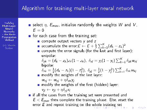
select η, Emax , initialise randomly the weights W and V ,

E = 0for each case from the training set:

compute output vectors y and z

accumulate the error:E ← E + 1

2

∑K

k=1(dk − zk)2

compute the error signals (for the last and �rst layer):unipolar:δzk = (dk − zk)zk(1− zk), δyj = yj(1− yj)

∑K

k=1δzkwkj

bipolar:δzk = 1

2(dk − zk)(1− z2k ), δyj = 1

2(1− y2j )

∑K

k=1δzkwkj

modify the weights of the last layer:wkj ← wkj + ηδzkyjmodify the weights of the �rst (hidden) layer:vji ← vji + ηδyjxi

if all the cases from the training set were presented andE < Emax then complete the training phase. Else, reset theerror E and repeat training on the whole training set

TrainingMulti-Layer

NeuralNetworks- the Back-PropagationMethod

(c) MarcinSydow

Summary

training single neuron with continuous activation function

training 1-layer of continuous neurons

training multi-layer network - back-propagation method

TrainingMulti-Layer

NeuralNetworks- the Back-PropagationMethod

(c) MarcinSydow

Thank you for attention.