Training Deep Networks with Structured Layers byMatrix Backpropagation∗

Catalin Ionescu†2,3, Orestis Vantzos‡3, and Cristian Sminchisescu§1,2

1Department of Mathematics, Faculty of Engineering, Lund University2Institute of Mathematics of the Romanian Academy

3Institute for Numerical Simulation, University of Bonn

April 15, 2016

Abstract

Deep neural network architectures have recently produced excellent results in a variety of areas in artificialintelligence and visual recognition, well surpassing traditional shallow architectures trained using hand-designedfeatures. The power of deep networks stems both from their ability to perform local computations followed bypointwise non-linearities over increasingly larger receptive fields, and from the simplicity and scalability of thegradient-descent training procedure based on backpropagation. An open problem is the inclusion of layers thatperform global, structured matrix computations like segmentation (e.g. normalized cuts) or higher-order pooling(e.g. log-tangent space metrics defined over the manifold of symmetric positive definite matrices) while preservingthe validity and efficiency of an end-to-end deep training framework. In this paper we propose a sound mathematicalapparatus to formally integrate global structured computation into deep computation architectures. At the heart ofour methodology is the development of the theory and practice of backpropagation that generalizes to the calculusof adjoint matrix variations. The proposed matrix backpropagation methodology applies broadly to a variety ofproblems in machine learning or computational perception. Here we illustrate it by performing visual segmentationexperiments using the BSDS and MSCOCO benchmarks, where we show that deep networks relying on second-orderpooling and normalized cuts layers, trained end-to-end using matrix backpropagation, outperform counterparts thatdo not take advantage of such global layers.

1 IntroductionRecently, the end-to-end learning of deep architectures using stochastic gradient descent, based on very large datasets,has produced impressive results in realistic settings, for a variety of computer vision and machine learning domains[2,3, 4, 5]. There is now a renewed enthusiasm of creating integrated, automatic models that can handle the diverse tasksassociated with an able perceiving system.

One of the most widely used architecture is the convolutional network (ConvNet) [6, 2], a deep processing modelbased on the composition of convolution and pooling with pointwise nonlinearities for efficient classification andlearning. While ConvNets are sufficiently expressive for classification tasks, a comprehensive, deep architecture, thatuniformly covers the types of structured non-linearities required for other calculations has not yet been established.In turn, matrix factorization plays a central role in classical (shallow) algorithms for many different computer visionand machine learning problems, such as image segmentation [7], feature extraction, descriptor design [8, 9], structurefrom motion [10], camera calibration [11], and dimensionality reduction [12, 13], among others. Singular valuedecomposition (SVD) in particular, is extremely popular because of its ability to efficiently produce global solutionsto various problems.

In this paper we propose to enrich the dictionary of deep networks with layer generalizations and fundamentalmatrix function computational blocks that have proved successful and flexible over years in vision and learning mod-els with global constraints. We consider layers which are explicitly structure-aware in the sense that they preserveglobal invariants of the underlying problem. Our paper makes two main mathematical contributions. The first showshow to operate with structured layers when learning a deep network. For this purpose we outline a matrix general-ization of backpropagation that offers a rigorous, formal treatment of global properties. Our second contribution is tofurther derive and instantiate the methodology to learn convolutional networks for two different and very successfultypes of structured layers: 1) second-order pooling [9] and 2) normalized cuts [7]. An illustration of the resulting∗This is an extended version of the ICCV 2015 article [1]†catalin.ionescu@ins.uni-bonn.de‡orestis.vantzos@ins.uni-bonn.de§cristian.sminchisescu@math.lth.se

1

arX

iv:1

509.

0783

8v4

[cs

.CV

] 1

4 A

pr 2

016

f (1) f (l)

x0

x1

...

xl

F=

UΣ

log(FTF+εI)xl+1

=

f (l+1) LlogSVD

...

xK

Figure 1: Overview of the DeepO2P recognition architecture made possible by our methodology. The levels 1 . . . lrepresent standard convolutional layers. Layer l + 1 is the global matrix logarithm layer presented in the paper. Thisis followed by fully connected layers and a logistic loss. The methodology presented in the paper enables analyticcomputation over both local and global layers, in a system that remains trainable end-to-end, for all its local andglobal parameters, using matrix variation generalizations entitled matrix backpropagation.

deep architecture for O2P is given in fig. 1. In challenging datasets like BSDS and MSCOCO, we experimentallydemonstrate the feasibility and added value of these two types of networks over counterparts that are not using globalcomputational layers.

2 Related WorkOur work relates to both the extensive literature in the area of (deep) neural networks (see [5] for a review) and with(shallow) architectures that have been proven popular and successful in machine learning and computer vision[7, 14,15, 16, 9]. While deep neural networks models have focused, traditionally, on generality and scalability, the shallowcomputer vision and machine learning architectures have often been designed with global computation and structuremodeling in mind. Our objective in this work is to provide first steps and one possible approach towards formallymarrying these two lines of work.

Neural networks in their modern realization can be traced back at least to [17]. The Perceptron [18] was thefirst two layer network, although limited in expressiveness. The derivation of backpropagation[19] and its furtheradvances more than a decade later [20, 21], allowed the development and the integration of new layers and the explo-ration of complex, more expressive architectures. This process lead to a successes in practical applications, e.g. fordigit recognition [6]. More recently, the availability of hardware, the large scale datasets [2], and the development ofcomplex enough architectures, lead to models that currently outperform all existing representations for challenging,general recognition problems. This recommends neural networks as one of the forefront methodologies for buildingrepresentations for prediction problems in computer vision and beyond[22]. [3] then showed that even more complex,deeper models can obtain even better results. This lead computer vision researchers to focus on transferring thissuccess to the detection and semantic segmentation problems, fields where handcrafted features[23, 24], statisticallyinspired[25, 26, 9] and deformable part models[27] were dominant at the time. R-CNN [28] uses standard networks(e.g. AlexNet [2] or VGG-16 [3]) to classify object proposals for detection. SDS [29] uses two input streams, one theoriginal image and the second the image with the background of the region masked each with AlexNet architecturesto take advantage of the shape information provided by the mask. He et al. [30, 31] propose a global spatial pyramidpooling layer before the fully connected layers, which perform simple max-pooling over pyramid-structured cells ofthe image. [32] uses committees to improve robustness and pushed performance close to, or beyond, human perfor-mance on tasks like traffic sign recognition and house number identification. In our first application we illustrate adeep architecture with a new log-covariance pooling layer that proved dominant for free-form region description [9],on top of manually designed local features such as SIFT. The methodology we propose makes it possible to deal withthe difficulties of learning the underlying features even in the presence such a complex intermediate representation.This part is also related to kernel learning approaches over the manifold of positive-definite matrices [33]. How-ever, we introduce different mathematical techniques related to matrix backpropagation, which has the advantages ofscalability and fitting together perfectly with existing deep network layers.

Among the first methods integrating structured models with CNNs is the work of [34] who showed that HMMscan be integrated into deep networks and showed results for speech and text analysis problems. [35] more recentlydemonstrated that using CRFs and deep networks can be trained end-to-end, showing strong results on digit recogni-tion and protein secondary structure prediction. Cast as a conditional random field (CRF) semantic segmentation hasalmost immediately taken advantage of the deep network revolution by providing useful smoothing on top of high-performing CNN pixel classifier predictions. [36] showed that the fully connected components, usually discarded byprevious methods, can also be made convolutional, i.e. the original resolution lost during pooling operations can berecovered by means a trained deconvolution layer. [37] obtained state-of-the-art semantic segmentation results usingan architecture similar to [36] but enforcing structure using globally connected CRFs[38] where only the unary poten-tials are learnt. Simultaneous work by [39] and [40] show that, since CRF mean field based approximate updates aredifferentiable, a fixed number of inference steps can be unrolled, the loss can be applied to them and then the gradientscan be backpropagated back first through the inference to the convolutional layers of the potentials. In [41] a more

2

efficient learning method is obtained by blending inference and training in order to obtain a procedure that updatesparameters as inference progresses. Unlike previous methods [42] learns CNN based pairwise potentials, separatefrom the CNN of the unary potential. Learning the model requires piece-wise training and minimizes an upper-boundon the CRF energy that decouples the potentials.

Our matrix backpropagation methodology generally applies to models that can be expressed as composed struc-tured non-linear matrix functions. As such, it can be applied to these deep models with a CRF top structure as wellwhere e.g. belief propagation in models with Gaussian potentials can be expressed as a solution to a linear system[43].While CRF-based methods designed on top of deep nets traditionally focus on iterative inference and learning wherein order to construct the derivatives of the final layer, one must combine the derivatives of each inference iterations,our methodology can be expressed in terms of invariants on the converged solution of linear systems – therefore itdoes not require iterative derivative calculations during inference.

Our second model used to illustrate the matrix backpropagation methodology, normalized cuts, has received lessattention from the deep network community as evidenced by the fact that leading methods are still handcrafted.Spectral formulations like normalized cuts(NCuts) [7] have obtained state-of-the-art results when used with strongpixel-level classifiers on top of hand-designed features[44]. A different approach is taken in [45] who show thatMRF inference can be relaxed to a spectral problem. Turaga et al [46] were the first to demonstrate the learning ofan image segmentation model end-to-end using CNN features, while optimizing a standard segmentation criterion.Learning and inference of NCuts was placed on firmer ground by Bach and Jordan [14] who introduced a (shallow)learning formulation which we build upon in this work with several important differences. First, it uses matrixderivatives, but makes appeal directly to the eigen-decompostion to derive them instead of projectors as we do. Thisallows them to truncate the spectrum and to consider only the eigenspace corresponding to the largest eigenvalues atthe cost of (potentially) making the criterion non-differentiable. We instead consider the entire eigenspace and relyon projectors (thus on the eigen-decomposition only indirectly) and aim to learn the dimensionality in the process.More importantly however, instead of learning parameters on top of fixed features as in [14], we directly learn theaffinity matrix by adapting the underlying feature representation, modeled as a deep network. The resulting method,combining strong pixel-level classifiers and a global (spectral) representation, can more naturally adapt pixel-level orsemi-local predictions for object detection and semantic segmentation, as these operations require not only structured,global computations, but also, for consistency, propagation of the information in the image. Careful application ofour methodology keeps the entire architecture trainable end-to-end. From another direction, in an effort to generalizeconvolutions to general non-Euclidean and non-equally spaced grids the work of [47] realizes the necessity of spectrallayers for learning the graph structure but since the computational issues brought on in the process are not the mainfocus, they do not handle them directly. In [48] such aspects are partially addressed but the authors focus on learningparameters applied to the eigenvalues instead of learning the eigenvectors and eigenvalues as we do. In this contextour focus is on the underlying theory of backpropagation when handling structured objects like matrices, allowingone to derive those and many other similar, but also more complex derivatives.

Symbolic matrix partial derivatives, one of the basis of our work, were first systematically studied in the seminalpaper [49]1, although not for complex non-linear layers like SVD or eigen-decomposition. Since then it has receivedinterest mainly in the context of studying estimators in statistics and econometrics [51]. Recently, the field of auto-matic differentiation has also shown interest in this theory when considering matrix functions[52]. This very powerfulmachinery has however appeared only scarcely in computer vision and machine learning. Some instances, althoughnot treating the general case, and focusing on the subset of the elements (variables) of interest, appeared in the contextof camera calibration[53], for learning parameters in a normalized cuts model[14], learning the parameters of Gaus-sian CRFs for denoising [43] and learning deep canonical correlation models [54]. The recent surge of interest in deepnetworks has exposed limitations of current compositional (layered) architectures based on local operations, whichin turn pushes the research in the direction of structured models requiring matrix based representations. Recently[55] multiplied the outputs of two networks as matrices, in order to obtain improved fine-grained recognition models,although the matrix derivatives in those case are straightforward. To our knowledge, we are the first to bring thismethodology, in its full generality, to the fore in the context of composed global non-linear matrix functions and deepnetworks, and to show promising results for two different computer vision and machine learning models.

Our methodological contributions are as follows: (a) the formulation of matrix back-propagation as a generalizedchain rule mechanism for computing derivatives of composed matrix functions with respect to matrix inputs (ratherthan scalar inputs, as in standard back-propagation), by relying on the theory of adjoint matrix variations; (b) theintroduction of spectral and non-linear (global structured) layers like SVD and eigen-decomposition which allow thecalculation of derivatives with respect to all the quantities of interest, in particular all the singular values and singularvectors or eigen-values and eigen-vectors, (c) the formulation of non-linear matrix function layers that take SVDor eigen-decompositions as inputs, with instantiations for second-order pooling models, (d) recipes for computingderivatives of matrix projector operations, instantiated for normalized-cuts models. (e) The novel methodology (a)-(d) applies broadly and is illustrated for end-to-end visual learning in deep networks with very competitive results.

1With few additions from disparate sources, these are the matrix derivatives results catalogued in the collection of matrix identities called “TheMatrix Cookbook”[50].

3

Paper organization: In the next section §3 we briefly present the main elements of the current deep network models.In §4.2 we outline the challenges and a computational recipe to handle matrix layers. §5 presents a “matrix function”layer using either SVD or an EIG decomposition and instantiated these to build deep second-order pooling models.In §6, we introduce an in-depth treatment to learn deep normalized cuts models. The experiments are presented in §7.

3 Deep Processing NetworksLet D = (d(i),y(i))i=1...N be a set of data points (e.g. images) and their corresponding desired targets (e.g. classlabels) drawn from a distribution p(d,y). Let L : Rd → R be a loss function i.e. a penalty of mismatch between themodel prediction function f : RD → Rd with parameters W for the input d i.e. f(d(i),W ) and the desired outputy(i). The foundation of many learning approaches, including the ones considered here, is the principle of empiri-cal risk minimization, which states that under mild conditions, due to concentration of measure, the empirical riskR(W ) = 1

N

∑Ni=1 L(f(d(i),W ),y(i)) converges to the true risk R(W ) =

∫L(f(d,W ),y)p(d,y). This implies

that it suffices to minimize the empirical risk to learn a function that will do well in general i.e.

arg minW

1

N

N∑i=1

L(f(d(i),W ),y(i)) (1)

If L and f are both continuous (though not necessarily with continuous derivatives) one can use (sub-)gradient descenton (1) for learning the parameters. This supports a general and effective framework for learning provided that a (sub-)gradient exists.

Deep networks, as a model, consider a class of functions f , which can be written as a series of successive functioncompositions f = f (K) f (K−1) . . . f (1) with parameter tuple W = (wK ,wK−1, . . . ,w1), where f (l) are calledlayers, wl are the parameters of layer l and K is the number of layers. Denote by L(l) = L f (K) . . . f (l) the lossas a function of the layer xl−1. This notation is convenient because it conceptually separates the network architecturefrom the layer design.

Since the computation of the gradient is the only requirement for learning, an important step is the effectiveuse of the principle of backpropagation (backprop). Backprop, as described in the literature, is an algorithm toefficiently compute the gradient of the loss with respect to the parameters, in the case of layers where the outputscan be expressed as vectors of scalars, which in the most general form, can individually be expressed as non-linearfunctions of the input. The algorithm recursively computes gradients with respect to both the inputs to the layers andtheir parameters (fig. 2) by making use of the chain rule. For a data tuple (d,y) and a layer l this is computing

∂L(l)(xl−1,y)

∂wl=∂L(l+1)(xl,y)

∂xl

∂f (l)(xl−1)

∂wl(2)

∂L(l)(xl−1,y)

∂xl−1=∂L(l+1)(xl,y)

∂xl

∂f (l)(xl−1)

∂xl−1(3)

where xl = f (l)(xl−1) and x0 = d (data). The first expression is the gradient we seek (required for updating wl)whereas the second one is necessary for calculating the gradients in the layers below and updating their parameters.

4 Structured Layers

The existing literature concentrates on layers of the form f (l) = (f(l)1 (xl−1), . . . , f

(l)dl+1

(xl−1)), where f (l)j : Rdl →

R, thus f (l) : Rdl → Rdl+1 . This simplifies processing significantly because in order to compute∂L(l)(xl−1,y)

∂xl−1

there is a well defined notion of partial derivative with respect to the layer∂f (l)(xl−1)

∂xl−1as well as a simple expression

for the chain rule, as given in (2) and (3). However this formulation processes spatial coordinates independently anddoes not immediately generalize to more complex mathematical objects.

Consider a matrix view of the (3-dimensional tensor) layer, X = xl−1, where Xij ∈ R, with i being the spatialcoordinate2 and j the index of the input feature. Then we can define a non-linearity on the entire X ∈ Rml×dl , as amatrix, instead of each (group) of spatial coordinate separately. As the matrix derivative with respect to a vector (setaside to a matrix) is no longer well-defined, a matrix generalization of backpropation is necessary.

For clarity, one has to draw a distinction between the data structures used to represent the layers and the mathemat-ical and computational operations performed. For example a convolutional neural network layer can be viewed, underthe current implementations, as a tensor where two dimensions correspond to spatial coordinates and one dimensioncorresponds to features. However, all mathematical calculations at the level of layers (including forward processing

2For simplicity and without loss of generality we reshape (linearize) the tensor’s spatial indices to one dimension with ml coordinates.

4

Figure 2: Deep architecture where data x and targets y are fed to a loss function L, via successively composedfunctions f (l) with parameters wl. Backpropagation (blue arrows) recursively expresses the partial derivative of theloss L w.r.t. the current layer parameters based on the partial derivatives of the next layer, cfeq. 2.

or derivative calculations) are not expressed on tensors. Instead these are performed on vectors and their scalar out-puts are used to selectively index and fill the tensor data structures. In contrast, a genuine matrix calculus would notjust rely on matrices as data structures, but use them as first class objects. This would require a coherent formulationwhere non-linear structured operations like forward propagation or derivative calculations are directly expressed usingmatrices. The distinction is not stylistic, as complex matrix operations for e.g. SVD or eigen-decomposition and theirderivatives simply cannot be implemented as index-filling.

4.1 Computer Vision ModelsTo motivate the use of structured layers we will consider the following two models from computer vision:

1. Second-Order Pooling is one of the competitive hand-designed feature descriptors for regions [9] used in thetop-performing method of the PASCAL VOC semantic segmentation, comp. 5 track [56, 57]. It representsglobal high-order statistics of local descriptors inside each region by computing a covariance matrix F>F ,where F ∈ Rm×d is the matrix of image features present in the region at the m spatial locations with d featuredimensions, then applying a tangent space mapping [58] using the matrix logarithm, which can be computedusing SVD. Instead of pooling over hand-designed local descriptors, such as SIFT [59], one could learn a deepfeature extractor (e.g. ConvNet) end-to-end, with an upper second-order pooling structured layer of the form

C = log(F>F + εI) (4)

where εI is a regularizer preventing log singularities around 0 when the covariance matrix is not full rank.

2. Normalized Cuts is an influential global image segmentation method based on pairwise similarities [7]. Itconstructs a matrix of local interactions W = FF>, where F ∈ Rm×d is a similar feature matrix with mspatial locations and d dimensions in the descriptor, then solves a generalized eigenvalue problem to determinea global image partitioning. Instead of manually designed affinities, one could, given a ground truth targetsegmentation, learn end-to-end the deep features that produce good normalized cuts.

4.2 Matrix BackpropagationWe call matrix backpropagation (MBP) the use of matrix calculus[49, 51, 52] to map between the partial derivatives∂L(l+1)

∂xland

∂L(l)

∂xl−1at two consecutive structured layers. Note that since for all layers l the function L(l) maps to real

numbers, by construction, both derivatives are well defined. In this section we simplify notation writing L = L(l+1),X,Y are the matrix versions of xl and xl−1 respectively, f = f (l) thus f(X) = Y .

The basis for the derivation is best understood starting from the Taylor expansion of the matrix functions[51] atthe two layers

L f(X + dX)− L f(X) =∂L f∂X

: dX + O(‖dX‖2) (5)

L(Y + dY )− L(Y ) =∂L

∂Y: dY + O(‖dY ‖2) (6)

where we introduced the notation A : B = Tr(A>B) = vec(A)> vec(B) for convenience. Thus A : B is an innerproduct in the Euclidean vec’d matrix space.

Our strategy of derivation, outlined below, involves two important concepts. A variation corresponds to theforward sensitivity and allows the easy manipulation of the first and higher order terms of a Taylor expansion. E.g.for a matrix function g we write dg = dg(X; dX) = g(X + dX)− g(X) = A(X) : dX +O(‖dX‖2), with A(X) amatrix of the same size as X and depending on X but not on dX . The (partial) derivative is by definition the linear‘coefficient’ of a Taylor expansion i.e. the coefficient of dX ergo ∂g

∂X = A(X). The variation and the partial derivativeare very different objects: dg is always defined if g is defined, it can take matrix inputs, and can map to a space ofmatrices. In contrast, the partial derivative also makes sense when g has matrix inputs, but is only defined when g has

5

scalar co-domain (image)3. The variation is used for the convenience of the derivation and needs not be implementedin practice. What we are ultimately after, for the purpose of matrix backpropagation, is the partial derivative.

The important element to understand is that when

dY = df(X; dX) (7)

the expressions (5) and (6) should be equal, since they both represent the variation of L for a given perturbation dXof the variable X . The first order terms of the Taylor expansions should also match, which gives us the chain rule

∂L f∂X

: dX =∂L

∂Y: dY (8)

The aim is to use this identity to express the partial derivative of the left hand side as a function of the partial derivativein the right hand side. The general recipe for our derivation follows two steps4:

1. Derive the functional L describing the variations of the upper layer variables with respect to the variations ofthe lower layer variables

dY = L(dX) , df(X; dX) (9)

The derivation of the variation involves not only the forward mapping of the layer, f (l), but also the invariantsassociated to its variables. If X satisfies certain invariants, these need to be preserved to first (leading) orderwhen computing dX . Invariants such as diagonality, symmetry, or orthogonality need to be explicitly enforcedin our methodology, by means of additional equations (constraints) beyond (9).

2. Given dY produced in step 1 above, we know that (8) holds. Thus we can use the properties of the matrix innerproduct A : B = Tr(A>B) to obtain the partial derivatives with respect to the lower layer variables. Since the“:” operator is an inner product on the space of matrices, this is equivalent to constructively producing L∗, anon-linear adjoint operator5 of L

∂L

∂Y: dY =

∂L

∂Y: L(dX) , L∗

(∂L

∂Y

): dX ⇒ L∗

(∂L

∂Y

)=∂L f∂X

(by the chain rule) (10)

This holds for a general variation, e.g. for a non-symmetric dX even ifX itself is symmetric. To remain withina subspace like the one of symmetric, diagonal or orthogonal matrices, we consider a projection of dX ontothe space of admissible variations and then transfer the projection onto the derivative, to obtain the projectedgradient. We use this technique repeatedly in our derivations.

Summarizing, the objective of our calculation is to obtain ∂Lf∂X . Specifically, we will compute ∂L

∂Y (typically back-propagated from the layer above) and dY = L(dX), then process the resulting expression using matrix identities, inorder to obtain an analytic expression for ∂L

∂Y : L(dX). In turn, extracting the inner product terms L∗(∂L∂Y

): dX

from that expression, allows us to compute L∗.

5 Spectral and Non-Linear LayersWhen global matrix operations are used in deep networks, they compound with other processing layers performedalong the way. Such steps are architecture specific, although calculations like spectral decomposition are widespread,and central, in many vision and machine learning models. SVD possesses a powerful structure that allows one toexpress complex transformations like matrix functions and algorithms in a numerically stable form. In the sequel weshow how the widely useful singular value decomposition (SVD) and the symmetric eigenvalue problem (EIG) canbe leveraged towards constructing layers that perform global calculations in deep networks.

5.1 Spectral LayersThe SVD layer receives a matrix X as input and produces a tuple of 3 matrices U ,Σ and V . Under the notationabove, this means Y = f(X) = (U,Σ, V ). The matrices satisfy the regular invariants of the SVD decompositioni.e. X = UΣV >, U>U = I , V >V = I and Σ is diagonal which will be taken into account in the derivation. Thefollowing proposition gives the variations of the outputs i.e. L(dX) = dY = (dU, dΣ, dV ) and the partial derivative

with respect to the layer∂L f∂X

as a function of the partial derivatives of the outputs ∂L∂Y , i.e.

∂L

∂U,∂L

∂Σand

∂L

∂V. Note

that these correspond, respectively, to the first and second step of the methodology presented in §4.2. In the sequel,we denote Asym = 1

2 (A> +A) and Adiag be A with all off-diagonal elements set to 0.

3See [51] for an in-depth treatment including questions about existence and uniqueness of the partial derivatives of matrix functions.4The appendices contain some of the basic identities used in each of these steps.5For arguments a, b, the adjoint operator L∗ of L is defined as having the property that a : L(b) = L∗(a) : b.

6

Proposition 1 (SVD Variations). Let X = UΣV > with X ∈ Rm,n and m ≥ n, such that U>U = I , V >V = I andΣ possessing diagonal structure. Then

dΣ = (U>dXV )diag (11)

anddV = 2V

(K> (Σ>U>dXV )sym

)(12)

with

Kij =

1

σ2i − σ2

j

, i 6= j

0, i = j(13)

Let Σn ∈ Rn×n be the top n rows of Σ and consider the block decomposition dU =(dU1 | dU2

)with dU1 ∈

Rm×n and dU2 ∈ Rm×m−n and similarly∂L

∂U=

((∂L

∂U

)1

∣∣∣∣ ( ∂L∂U)

2

), where

(∂L

∂U

)1

∈ Rm×n and(∂L

∂U

)2

∈

Rm×m−n. ThendU =

(CΣ−1

n | − U1Σ−1n C>U2

)(14)

withC = dXV − UdΣ− UΣdV >V (15)

Consequently the partial derivatives are

∂L f∂X

= DV > + U

(∂L

∂Σ− U>D

)diag

V > + 2UΣ

(K>

(V >

(∂L

∂V− V D>UΣ

)))sym

V > (16)

where

D =

(∂L

∂U

)1

Σ−1n − U2

(∂L

∂U

)>2

U1Σ−1n (17)

Proof. Let X = UΣV > by way of SVD, with X ∈ Rm×n and m ≥ n, Σ ∈ Rm×n diagonal and U ∈ Rm×m,V ∈ Rn×n orthogonal. For a given variation dX of X , we want to calculate the variations dU ,dΣ and dV . Thevariation dΣ is diagonal, like Σ, whereas dU and dV satisfy (by orthogonality) the constraints U>dU + dU>U = 0and V >dV + dV >V = 0 respectively. Taking the first variation of the SVD decomposition, we have

dX = dUΣV > + UdΣV > + UΣdV > (18)

then, by using the orthogonality of U and V , it follows that

⇒U>dXV = U>dUΣ + dΣ + ΣdV >V ⇒⇒R = AΣ + dΣ + ΣB

with R = U>dXV and A = U>dU , B = dV >V both antisymmetric. Since dΣ is diagonal whereas AΣ, ΣBhave both zero diagonal, we conclude that

dΣ = (U>dXV )diag (19)

The off-diagonal part then satisfies

AΣ + ΣB = R−Rdiag ⇒ Σ>AΣ + Σ>ΣB = Σ>(R−Rdiag) = Σ>R

⇒

σiaijσj + σ2

i bij = σiRij

−σjaijσi − σ2j bij = σjRji (A,B antisym.)

⇒ (σ2i − σ2

j )bij = σiRij + Rjiσj ⇒ bij =

(σ2

i − σ2j )−1

(σiRij + Rjiσj

), i 6= j

0 , i = j(20)

where σi = Σii and R = R−Rdiag . We can write this as B = K (Σ>R+ R>Σ) = K (Σ>R+R>Σ), where

Kij =

1

σ2i − σ2

j

, i 6= j

0, i = j(21)

Finally,dV = V B> ⇒ dV = 2V

(K> (Σ>U>dXV )sym

)(22)

Note that this satisfies the condition V >dV + dV >V = 0 by construction, and so preserves the orthogonality of V toleading order.

7

Using the dΣ and dV we have obtained, one can obtain dU from the variations of dX in (18):

dX = dUΣV > + UdΣV > + UΣdV > ⇒ dUΣ = dXV − UdΣ− UΣdV >V =: C

This equation admits any solution of the block form dU =(dU1 dU2

), where dU1 := CΣ−1

n ∈ Rm×n (Σn being thetop n rows of Σ) and dU2 ∈ Rm×m−n arbitrary as introduced in the proposition. To determine dU2 uniquely we turnto the orthogonality condition

dU>U + U>dU = 0⇒(dU>1 U1 + U>1 dU1 dU>1 U2 + U>1 dU2

dU>2 U1 + U>2 dU1 dU>2 U2 + U>2 dU2

)= 0

The block dU1 already satisfies the top left equation, so we look at the top right (which is equivalent to bottom left).Noting that U>1 U1 = I by the orthogonality of U , we can verify that dU2 = −U1dU

>1 U2. Since this also satisfies the

remaining equation, orthogonality is satisfied. Summarizing

dU =(CΣ−1

n | − U1Σ−1n C>U2

), C = dXV − UdΣ− UΣdV >V (23)

We proceed further with the second part of the matrix backpropagation to compute∂L f∂X

. Note that the chain

rule in this case is∂L f∂X

: dX =∂L

∂U: dU +

∂L

∂Σ: dΣ +

∂L

∂V: dV . We can replace dU , dV and dΣ with their

expressions w.r.t. dX to obtain the partial derivatives.Before computing the full derivatives we simplify slightly the expression corresponding to dU

∂L

∂U: dU =

(∂L

∂U

)1

: CΣ−1n +

(∂L

∂U

)2

: −U1Σ−1n C>U2 (24)

=

(∂L

∂U

)1

Σ−1n : C − Σ−1

n U>1

(∂L

∂U

)2

U>2 : C> (25)

=

(∂L

∂U

)1

Σ−1n : C − U2

(∂L

∂U

)>2

U1Σ−1n : C (26)

=

((∂L

∂U

)1

Σ−1n − U2

(∂L

∂U

)>2

U1Σ−1n

): (dXV − UdΣ− UΣdV >V ) (27)

= D : dXV −D : UdΣ−D : UΣdV >V (28)

= DV > : dX − U>D : dΣ− ΣU>DV > : dV > (29)

= DV > : dX − U>D : dΣ− V D>UΣ : dV (30)

Now we can plug this result in the full derivative

∂L

∂U: dU +

∂L

∂Σ: dΣ +

∂L

∂V: dV =(DV > : dX − U>D : dΣ− V D>UΣ : dV ) +

∂L

∂Σ: (U>dXV )diag+

+∂L

∂V:

2V(K> (Σ>U>dXV )sym

)=DV > : dX +

(∂L

∂Σ− U>D

): (U>dXV )diag+

+

(∂L

∂V− V D>UΣ

):

2V(K> (Σ>U>dXV )sym

)=DV > : dX +

(∂L

∂Σ− U>D

)diag

: (U>dXV )+

+ 2V >(∂L

∂V− V D>UΣ

):(K> (Σ>U>dXV )sym

)by (68), (69)

=DV > : dX + U

(∂L

∂Σ− U>D

)diag

V > : dX+

+ 2

(K>

(V >

(∂L

∂V− V D>UΣ

)))sym

: Σ>U>dXV by (70),(71)

=DV > : dX + U

(∂L

∂Σ− U>D

)diag

V > : dX+

+ 2UΣ

(K>

(V >

(∂L

∂V− V D>UΣ

)))sym

V > : dX by (68)

8

and so, since the last expression is equal to∂L f∂X

: dX by the chain rule,

∂L f∂X

= DV > + U

(∂L

∂Σ− U>D

)diag

V > + 2UΣ

(K>

(V >

(∂L

∂V− V D>UΣ

)))sym

V > (31)

The EIG is a layer that receives a matrix X as input and produces a pair of matrices U and Σ. Given ournotation, this means Y = f(X) = (U,Σ). The matrices satisfy the regular invariants of the eigen-decompositioni.e. X = UΣU>, U>U = I and Σ is a diagonal matrix. The following proposition identifies the variations of the

outputs i.e. L(dX) = dY = (dU, dΣ) and the partial derivative with respect to this layer∂L f∂X

as a function of the

partial derivatives of the outputs∂L

∂Yi.e.

∂L

∂Uand

∂L

∂Σ.

Proposition 2 (EIG Variations). Let X = UΣU> with X ∈ Rm,m, such that U>U = I and Σ possessing diagonalstructure. Then

dΣ = (U>dXU)diag (32)

anddU = U

(K> (U>dXU)

)(33)

with

Kij =

1

σi − σj, i 6= j

0, i = j(34)

The resulting partial derivatives are

∂L f∂X

= U

(K>

(U>

∂L

∂U

))+

(∂L

∂Σ

)diag

U> (35)

Proof. First note that (19) still holds and with the notation above we have in this case m = n, U = V . This implies

dΣ = (U>dXU)diag (36)

Furthermore we have A = B> (A, B antisymmetric) and the off-diagonal part then satisfies AΣ + ΣA> =R−Rdiag . In a similar process with the asymmetric case, we have

AΣ + ΣA> = R − Rdiag ⇒ AΣ − ΣA = R ⇒

aijσj − aijσi = Rij , i 6= j

aij = 0, i = j

so that A = K> R with

Kij =

1

σi − σj, i 6= j

0, i = j(37)

From this, we get thendU = U

(K> (U>dXU)

)(38)

Note that the chain rule in this case is∂L f∂X

: dX =∂L

∂U: dU +

∂L

∂Σ: dΣ, we can replace dU and dΣ with

their expressions w.r.t. dX to obtain the partial derivatives

∂L

∂U: dU +

∂L

∂Σ: dΣ =

∂L

∂U:U(K>

(U>dXU

))+∂L

∂Σ:(U>dXU

)diag

= U

(K>

(U>

∂L

∂U

))U> : dX + U

(∂L

∂Σ

)diag

U> : dX

and so∂L f∂X

= U

(K>

(U>

∂L

∂U

))+

(∂L

∂Σ

)diag

U> (39)

Note that (19), (38), (37) and (39) represent the desired quantities of the proposition.

9

5.2 Non-Linear LayersUsing the SVD and EIG layers presented above we are now ready to produce layers like O2P that involve matrixfunctions g, e.g. g = log, but that are learned end-to-end. To see how, consider the SVD of some deep featurematrix F = UΣV > and notice that g(F>F + εI) = g(V Σ>U>UΣV > + εV V >) = V g(Σ>Σ + εI)V >, wherethe last equality is obtained from the definition of matrix functions given that Schur decomposition and the eigen-decomposition coincide for real symmetric matrices[60]. Thus to implement the matrix function, we can create a newlayer that receives the outputs of the SVD layer and produces V g(Σ>Σ+εI)V >, where g is now applied element-wiseto the diagonal elements of Σ>Σ + εI thus is much easier to handle.

An SVD matrix function layer receives as input a tuple of 3 matrices U ,Σ and V and produces the responseC = V g(Σ>Σ + εI)V >, where g is an analytic function and ε is a parameter that we consider fixed for simplicity.With the notation in section §4.2 we have X = (U,Σ, V ) and Y = f(X) = V g(Σ>Σ + εI)V >. The followingproposition gives the variations of the outputs are i.e. L(dX) = dY = dC and the partial derivatives with respect

to this layer∂L f∂X

i.e.(∂L f∂V

,∂L f∂Σ

)as a function of the partial derivatives of the outputs

∂L

∂C. Note that the

layer does not depend on U so its derivative∂L

∂U= 0.

Proposition 3 (SVD matrix function). An (analytic) matrix function of a diagonalizable matrix A = V ΣV > canbe written as g(A) = V g(Σ)V >. Since Σ is diagonal this is equivalent to applying g element-wise to Σ’s diagonalelements. Combining this idea with the SVD decomposition F = UΣV >, our matrix function can be written asC = g(F>F + εI) = V g(Σ>Σ + εI)V >.

Then the variations are

dC = 2(dV g(Σ>Σ + εI)V >

)sym

+ 2(V g′(Σ>Σ + εI)Σ>dΣV >

)sym

and the partial derivatives are∂L f∂V

= 2

(∂L

∂C

)sym

V g(Σ>Σ + εI) (40)

and∂L f∂Σ

= 2Σg′(Σ>Σ + εI)V >(∂L

∂C

)sym

V (41)

Proof. Using the fact that for a positive diagonal matrix A and a diagonal variation dA, g(A + dA) = g(A) +g′(A)dA+ O(‖dA‖2), we can write

dC = 2(dV g(Σ>Σ + εI)V

)sym

+ 2(V g′(Σ>Σ + εI)Σ>dΣV >

)sym

The total variation dL of an expression of the form L = g(C), g : Rn×n → Rn×n, can then be written as:

∂L

∂C: dC =

∂L

∂C:

2(dV g(Σ>Σ + εI)V >

)sym

+ 2(V g′(Σ>Σ + εI)Σ>dΣV >

)sym

=2

(∂L

∂C

)sym

: (dV g(Σ>Σ + εI)V >) + 2

(∂L

∂C

)sym

: (V g′(Σ>Σ + εI)Σ>dΣV >) by (70)

=2

(∂L

∂C

)sym

V g(Σ>Σ + εI)

: dV + 2

Σg′(Σ>Σ + εI)V >

(∂L

∂C

)sym

V

: dΣ by (68)

By the chain rule, we must have

∂L

∂C: dC =

∂L f∂V

: dV +∂L f∂Σ

: dΣ ⇒

∂Lf∂V = 2

(∂L∂C

)sym

V g(Σ>Σ + εI)∂Lf∂Σ = 2Σg′(Σ>Σ + εI)V >

(∂L∂C

)sym

V(42)

Similarly the EIG matrix function layer receives as input a pair of matrices U and Q and produces the responseC = Ug(Q)U>. With the notation from §4.2 we have X = (U,Q) and Y = f(X) = Ug(Q)U>. Note that ifthe inputs obey the invariants of the EIG decomposition of some real symmetric matrix Z = UQU> i.e. U are theeigenvectors and Q the eigenvalues, then the layer produces the result of the matrix function C = g(Z). This holdsfor similar reasons as above g(Z) = g(UQU>) = Ug(Q)U>, since in this case the Schur decomposition coincideswith the eigen-decomposition [60]. The following proposition shows what the variations of the outputs are in this case

i.e. L(dX) = dY = dC and what the partial derivatives with respect to this layer are∂L f∂X

i.e.(∂L f∂U

,∂L f∂Q

)as a function of the partial derivatives of the outputs

∂L

∂C.

10

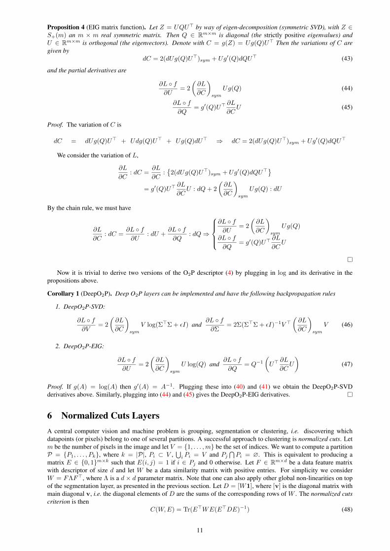
Proposition 4 (EIG matrix function). Let Z = UQU> by way of eigen-decomposition (symmetric SVD), with Z ∈S+(m) an m × m real symmetric matrix. Then Q ∈ Rm×m is diagonal (the strictly positive eigenvalues) andU ∈ Rm×m is orthogonal (the eigenvectors). Denote with C = g(Z) = Ug(Q)U> Then the variations of C aregiven by

dC = 2(dUg(Q)U>)sym + Ug′(Q)dQU> (43)

and the partial derivatives are

∂L f∂U

= 2

(∂L

∂C

)sym

Ug(Q) (44)

∂L f∂Q

= g′(Q)U>∂L

∂CU (45)

Proof. The variation of C is

dC = dUg(Q)U> + Udg(Q)U> + Ug(Q)dU> ⇒ dC = 2(dUg(Q)U>)sym + Ug′(Q)dQU>

We consider the variation of L,

∂L

∂C: dC =

∂L

∂C:

2(dUg(Q)U>)sym + Ug′(Q)dQU>

= g′(Q)U>∂L

∂CU : dQ+ 2

(∂L

∂C

)sym

Ug(Q) : dU

By the chain rule, we must have

∂L

∂C: dC =

∂L f∂U

: dU +∂L f∂Q

: dQ⇒

∂L f∂U

= 2

(∂L

∂C

)sym

Ug(Q)

∂L f∂Q

= g′(Q)U>∂L

∂CU

Now it is trivial to derive two versions of the O2P descriptor (4) by plugging in log and its derivative in thepropositions above.

Corollary 1 (DeepO2P). Deep O2P layers can be implemented and have the following backpropagation rules

1. DeepO2P-SVD:

∂L f∂V

= 2

(∂L

∂C

)sym

V log(Σ>Σ + εI) and∂L f∂Σ

= 2Σ(Σ>Σ + εI)−1V >(∂L

∂C

)sym

V (46)

2. DeepO2P-EIG:

∂L f∂U

= 2

(∂L

∂C

)sym

U log(Q) and∂L f∂Q

= Q−1

(U>

∂L

∂CU

)(47)

Proof. If g(A) = log(A) then g′(A) = A−1. Plugging these into (40) and (41) we obtain the DeepO2P-SVDderivatives above. Similarly, plugging into (44) and (45) gives the DeepO2P-EIG derivatives.

6 Normalized Cuts LayersA central computer vision and machine problem is grouping, segmentation or clustering, i.e. discovering whichdatapoints (or pixels) belong to one of several partitions. A successful approach to clustering is normalized cuts. Letm be the number of pixels in the image and let V = 1, . . . ,m be the set of indices. We want to compute a partitionP = P1, . . . , Pk, where k = |P|, Pi ⊂ V ,

⋃i Pi = V and Pj

⋂Pi = ∅. This is equivalent to producing a

matrix E ∈ 0, 1m×k such that E(i, j) = 1 if i ∈ Pj and 0 otherwise. Let F ∈ Rm×d be a data feature matrixwith descriptor of size d and let W be a data similarity matrix with positive entries. For simplicity we considerW = FΛF>, where Λ is a d × d parameter matrix. Note that one can also apply other global non-linearities on topof the segmentation layer, as presented in the previous section. Let D = [W1], where [v] is the diagonal matrix withmain diagonal v, i.e. the diagonal elements of D are the sums of the corresponding rows of W . The normalized cutscriterion is then

C(W,E) = Tr(E>WE(E>DE)−1) (48)

11

Finding the matrix E that minimizes C(W,E) is equivalent to finding a partition that minimizes the cut energy butpenalizes unbalanced solutions.

It is easy to show[14] that C(W,E) = k−Tr(Z>D−1/2WD−1/2Z), where Z is such that: a) Z>Z = I , and b)D1/2Z is piecewise constant with respect toE (i.e. it is equal toE times some scaling for each column). Ignoring thesecond condition we obtain a relaxed problem that can be solved, due to Ky Fan theorem, by an eigen-decompositionof

M = D−1/2WD−1/2 (49)

[14] propose to learn the parameters Λ such that D1/2Z is piecewise constant because then, solving the relaxedproblem is equivalent to the original problem. In [14] the input features were fixed, thus Λ are the only parameters topermit the alignment. This is not our case, as we place a global objective on top of convolutional network inputs. Wecan can therefore take leverage the network parameters in order to change F directly, thus training the bottom layersto produce a representation that is appropriate for normalized cuts.

To obtain a Z that is piecewise constant with respect to D1/2E we can align the span of M with that of Ω =D1/2EE>D1/2. For this we can use projectors ΠA of the corresponding space spanned by A, where ΠA = AA+

is an orthogonal projector and A+ is the Moore-Penrose inverse of A. The alignment is achieved by minimizing theFrobenius norm of the projectors associated to the the model prediction ΠM and the desired output ΠΩ, respectively

J1(W,E) =1

2‖ΠM −ΠΩ‖2F (50)

Notice that while our criterion J1 is superficially similar to the one in [14], there are important differences. [14]truncate the spectrum and consider only the eigenspace corresponding to the largest eigenvalues at the cost of (poten-tially) making the criterion non-differentiable. In contrast, we consider the entire eigenspace and rely on projectors(and only indirectly on eigen-decomposition) aiming to also learn the dimensionality of the space in the process.

We will obtain the partial derivatives of an objective with respect to the matrices it depends on, relying on matrixbackpropagation. Since the projectors will play a very important role in a number of different places in this sectionwe will treat them separately.

Consider a layer that takes a matrix A as input and produces its corresponding orthogonal projector ΠA = AA+.In the notation of section 4.2, X = A and Y = f(A) = ΠA. The following proposition gives the variations of the

outputs i.e. L(dX) = dY = dΠA and the partial derivative with respect to the layer∂L f∂X

as a function of the

partial derivatives of the outputs ∂L∂Y , i.e.

∂L

∂ΠA.

Lemma 1. Consider a symmetric matrixA and its orthogonal projection operator ΠA. If dA is a symmetric variationof A then

dΠA = 2((I −ΠA)dAA+

)sym

) (51)

and∂L f∂A

= 2(I −ΠA)

(∂L

∂ΠA

)sym

A+ (52)

Proof. (We drop the subscript of ΠA for brevity.) Taking the variation of the basic properties of the projector Π2 = Πand ΠA = A, we have

dΠΠ + ΠdΠ = dΠ (53)dΠA+ ΠdA = dA (54)

We then consider the following decomposition of dΠ

dΠ = ΠMΠ + (I −Π)QΠ + ΠQ>(I −Π) + (I −Π)R(I −Π)

with M and R symmetric, so that dΠ is symmetric by construction. Plugging into the equations above, we obtain

2ΠMΠ + (I −Π)QΠ + ΠQ>(I −Π) = dΠ

ΠMA+ (I −Π)QA = (I −Π)dA

Comparing the first equation with the decomposition of dΠ above, we infer that M = R = 0, and so

(I −Π)QΠ + ΠQ>(I −Π) = dΠ

(I −Π)QA = (I −Π)dA

Multiplying the second equation with A+ at the right hand side gives (I − Π)QΠ = (I − Π)dAA+. Plugging thisinto the first equation gives the desired result for the variations.

12

Now we can calculate the partial derivative

∂L

∂ΠA: dΠA = 2

(∂L

∂ΠA

)sym

: ((I −ΠA)dAA+) by (51)

= 2(I −ΠA)

(∂L

∂ΠA

)sym

A+ : dA

and so∂L f∂A

= 2(I −ΠA)

(∂L

∂ΠA

)sym

A+ (55)

The derivation relies only on basic properties of the projector with respect to itself and its matrix: Π2A = ΠA

(idempotency of the projector) and ΠAA = A (projector leaves the original space unchanged). Note that sinceΠA = AA+, there exists a non-trivial spectral decomposition in training, although it is ‘notationally’ hidden underA+, which nevertheless requires an SVD computation.

From the perspective of matrix backpropagation we split the computation of J1 into the following 4 layers F →W → (M,Ω) → (ΠM ,ΠΩ) → J1. We consider them in reverse order from the objective down to the inputs. First

the derivative of the Frobenius norm is well known[50] so∂J1

∂ΠM= ΠM −ΠΩ and

∂J1

∂ΠΩ= ΠΩ−ΠM . Then we focus

on the layer taking as inputs M or Ω and producing the corresponding projectors i.e. ΠM and ΠΩ. These derivativesare obtained by applying Lemma 1.

Subsequently, we consider the layer receiving (W,E) as inputs and producing (M,Ω). Under the notation intro-duced in §4.2, L = J1, X = (W,E) and Y = f(X) = (M,Ω) as defined above. The following proposition gives the

variations of the outputs i.e. L(dX) = dY = (dM, dΩ) and the partial derivative with respect to the layer∂L f∂X

as

a function of the partial derivatives of the outputs∂L

∂Yi.e.(∂L

∂M,∂L

∂Ω

).

Proposition 5. With the notation above, the variations of M and Ω are

dΩ =(ΩD−1[dW1]

)sym

(56)

anddM = D−1/2dWD−1/2 −

(MD−1[dW1]

)sym

(57)

and the partial derivative of J1 with respect to W is

∂J1 f∂W

= D−1/2 ∂J1

∂MD−1/2 + diag

(D−1Ω

(∂J1

∂Ω

)sym

−D−1M

(∂J1

∂M

)sym

)1>

Proof. For a diagonal matrix D under a diagonal variation dD, we can show that d(Dp) = pDp−1dD by means ofelement-wise differentiation. For the particular D = [W1], we have dD = [dW1]. Using these, we obtain

dΩ =1

2dDD−1/2EE>D1/2+

1

2D1/2EE>D−1/2dD =

(D1/2EE>D−1/2dD

)sym

=(ΩD−1[dW1]

)sym

(58)

and

dM = −1

2dDD−3/2WD−1/2 +D−1/2dWD−1/2 − 1

2D−1/2WD−3/2dD

= D−1/2dWD−1/2 −(MD−1[dW1]

)sym

Then, plugging in the variations we compute the partial derivative

∂J1

∂M: dM +

∂J1

∂Ω: dΩ =

(D−1/2 ∂J1

∂MD−1/2

): dW −

(D−1M

∂J1

∂M sym

): [dW1] +

(D−1Ω

∂J1

∂Ω sym

): [dW1]

then identifying we obtain

∂J1

∂W= D−1/2 ∂J1

∂MD−1/2 + diag

(D−1Ω

∂J1

∂Ω sym−D−1M

∂J1

∂M sym

)1>

where we used the property A : [Bx] = Aii(Bijxj) = (Aiixj)Bij =(diag(A)x>

): B.

13

A related optimization objective also presented in [14] is

J2 =1

2‖ΠW −ΠΨ‖2F , (59)

with Ψ = E(E>E)−1E>. Here we consider ΠW = V (V >V )−1V >, where V = D1/2U . We observe that this is aprojector for W by noting that ΠW = D1/2U(U>DU)−1U>D1/2 and M = UΣU> = D−1/2WD−1/2, by eigendecomposition and (49). Then indeed

1. Idempotency of ΠW

Π2W = D1/2U(U>DU)−1U>DU(U>DU)−1U>D1/2 = ΠW

2. ΠW leaves W unchanged

ΠWW = ΠW (D1/2MD1/2)

= D1/2U(U>DU)−1(U>DU)ΣU>D1/2

= D−1/2UΣU>D−1/2 = W

Proposition 6. The corresponding partial derivative∂J2

∂Wis

∂J2

∂W= −2(I −ΠW )ΠΨW

+ (60)

Proof. Since Ψ does not depend on W , then∂J2

∂Ψ= 0, so the derivation is much simpler

∂J2

∂W= −2(I −ΠW )

(∂J2

∂ΠW

)W+ by Lemma 1 (61)

= −2(I −ΠW )(ΠW −ΠΨ)W+ by Frobenius derivative (62)

= −2(I −ΠW )ΠΨW+ by idempotency of projector (63)

Finally, in both cases, we consider a layer that receives Λ and F as inputs and outputs the data similarityW = FΛF>. Following the procedure of section 4.2, first we compute the first order variations dW = dFΛF> +FdΛF> + FΛdF>. We then use the trace properties to make the partial derivatives identifiable

dJi =∂Ji∂W

: dW =∂Ji∂W

:(FdΛF>

)+ 2

∂Ji∂W

: (dFΛF>)sym

=

(F>

∂Ji∂W

F

): dΛ + 2

(∂Ji∂W sym

FΛ>)

: dF

Thus we obtain∂Ji∂Λ

= F>∂Ji∂W

F (64)

and∂Ji∂F

= 2

(∂Ji∂W

)sym

FΛ> (65)

Note that when J = J2 then∂J2

∂Λ= 0, since (I − ΠW )F = F>(I − ΠW ) = 0. Thus we cannot learn Λ

by relying on our projector trick, but there is no problem learning F , which is our objective, and arguably moreinteresting, anyway.

An important feature of our formulation is that we do not restrict the rank in training. During alignment, theoptimization may choose to collapse certain directions thus reducing rank. We prove a topological lemma implyingthat if the Frobenius distance between the projectors (such as in the two objectives J1, J2) drops below a certainvalue, then the ranks of the two projectors will match. Conversely, if for some reason the ranks cannot converge, theobjectives are bounded away from zero. The following lemma shows that when the projectors of two matrices A andB are close enough in the ‖·‖2 norm, then the matrices have the same rank.

Lemma 2. Let A,B ∈ Rm×n, and ΠA, ΠB their respective orthogonal projectors. If ‖ΠA − ΠB‖2 < 1 thenrankA = rankB.

14

Proof. The spectral norm ‖·‖2 can indeed be defined as ‖A‖2 = sup‖x‖2 6=0‖Ax‖‖x‖ . We assume that the ranks of A and

B are different, i.e. w.l.o.g. rankA > rankB. By the fundamental theorem of linear algebra there exists a vector vin the range of A (so that ΠAv = v), that is orthogonal to the range of B (so that ΠBv = 0). We have then

‖ΠA −ΠB‖2 ≥‖ΠAv −ΠBv‖

‖v‖=‖ΠAv‖‖v‖

= 1

which is a contradiction.

Given that the Frobenius norm controls the spectral norm, i.e. ‖A‖2 ≤ ‖A‖F (§2.3.2 of [60]), an immediatecorollary is that when J2 is bounded above by 1/2, then ||A||2 < 1 and the spaces spanned by W and EE> areperfectly aligned, i.e.

J2(W ) <1

2⇒ rank(W ) = rank(EE>) (66)

7 ExperimentsIn this section we validate the proposed methodology by constructing models on standard datasets for region-basedobject classification, like Microsoft COCO [61], and for image segmentation on BSDS [44]. A matconvnet [62]implementation of our models and methods is publicly available.

7.1 Region Classification on MSCOCOFor recognition we use the MSCOCO dataset [61], which provides 880k segmented training instances across 80classes, divided into training and validation sets. The main goal is to assess our second-order pooling layer in varioustraining settings. A secondary goal is to study the behavior of ConvNets learned from scratch on segmented trainingdata. This has not been explored before in the context of deep learning because of the relatively small size of thedatasets with associated object segmentations, such as PASCAL VOC [63].

The experiments in this section use the convolutional architecture component of AlexNet[2] with the global O2Players we propose in order to obtain DeepO2P models with both classification and fully connected (FC) layers in thesame topology as Alexnet. We crop and resize each object bounding box to have 200 pixels on the largest side, thenpad it to the standard AlexNet input size of 227x227 with small translation jittering, to limit over-fitting. We also ran-domly flip the images in each mini-batch horizontally, as in standard practice. Training is performed with stochasticgradient descent with momentum. We use the same batch size (100 images) for all methods but the learning rate wasoptimized for each model independently. All the DeepO2P models used the same ε = 10−3 parameter value in (4).

Method SIFT-O2P AlexNet AlexNet (S) DeepO2P DeepO2P(S) DeepO2P-FC DeepO2P-FC(S)Results 36.4 25.3 27.2 28.6 32.4 25.2 28.9

Table 1: Classification error on the validation set of MSCOCO (lower is better). Models with (S) suffixes were trainedfrom scratch (i.e. random initialization) on the MSCOCO dataset. The DeepO2P models only use a classificationlayer on top of the DeepO2P layer whereas the DeepO2P-FC also have fully connected layers in the same topologyas AlexNet. All parameters of our proposed global models are refined jointly, end-to-end, using the proposed matrixbackpropagation.

Architecture and Implementation details. Implementing the spectral layers efficiently is challenging since the GPUsupport for SVD is still very limited and our parallelization efforts even using the latest CUDA 7.0 solver API havedelivered a slower implementation than the standard CPU-based. Consequently, we use CPU implementations andincur a penalty for moving data back and forth to the CPU. The numerical experiments revealed that an implementationin single precision obtained a significantly less accurate gradient for learning. Therefore all computations in ourproposed layers, both in the forward and backward passes, are made in double precision. In experiments we stillnoticed a significant accuracy penalty due to inferior precision in all the other layers (above and below the structuredones), still computed in single precision, on the GPU.

The second formal derivation of the non-linear spectral layer based on an eigen-decomposition of Z = F>F + εIinstead of SVD of F is also possible but our numerical experiments favor the formulation using SVD. The alternativeimplementation, which is formally correct, exhibits numerical instability in the derivative when multiple eigenvalueshave very close values, thus producing blow up in K. Such numerical issues are expected to appear under someimplementations, when complex layers like the ones presented here are integrated in deep network settings.

Results. The results of the recognition experiment are presented in table 1. They show that our proposed DeepO2P-FC models, containing global layers, outperform standard convolutional pipelines based on AlexNet, on this problem.The bottom layers are pre-trained on ImageNet using AlexNet, and this might not provide the ideal initial input

15

Arch [45] AlexNet VGGLayer ReLU-5 ReLU-4 ReLU-5

Method NCuts NCuts DeepNCuts NCuts DeepNCuts NCuts DeepNCutsResults .55 (.44) .59 (.49) .65 (.56) .65 (.56) .73 (.62) .70 (.58) .74 (.63)

Table 2: Segmentation results give best and average covering to the pool of ground truth segmentations on theBSDS300 dataset [44] (larger is better). We use as baselines the original normalized cuts [45] using interveningcontour affinities as well as normalized cuts with affinities derived from non-finetuned deep features in different lay-ers of AlexNet (ReLU-5 - the last local ReLU before the fully connected layers) and VGG (first layer in block 4 andthe last one in block 5). Our DeepNCuts models are trained end-to-end, based on the proposed matrix backpropagationmethodology, using the objective J2.

features. However, despite this potentially unfavorable initialization, our model jointly refines all parameters (bothconvolutional, and corresponding to global layers), jointly, end to end, using a consistent cost function.

We note that the fully connected layers on top of the DeepO2P layer offer good performance benefits. O2P overhand-crafted SIFT performs considerably less well than our DeepO2P models, suggesting that large potential gainscan be achieved when deep features replace existing descriptors.

7.2 Full-Image Segmentation on BSDS300We use the BSDS300 dataset to validate our deep normalized cuts approach. BSDS contains 200 training images and100 testing images and human annotations of all the relevant regions in the image. Although small by the standardsof neural network learning it provides exactly the supervision we need to refine our model using global information.Note that since the supervision is pixel-wise, the number of effective datapoint constraints is much larger. We eval-uate using the average and best covering metric under the Optimal Image Scale (OIS) criterion [44]. Given a set offull image segmentations computed for an image, selecting the one that maximizes the average and best covering,respectively, compared to the pool of ground truth segmentations.

Architecture and Implementation details. We use both the AlexNet[2] and the VGG-16[3] architectures to feed ourglobal layers. All the parameters of the deep global models (including the low-level features, pretrained on ImageNet)are refined end-to-end. We use a linear affinity but we need all entries of W to be positive. Thus, we use ReLU layersto feed the segmentation ones. Initially, we just cascaded our segmentation layer to different layers in AlexNet butthe resulting models were hard to learn. Our best results were obtained by adding two Conv-ReLU pairs initializedrandomly before the normalized cuts layer. This results in many filters in the lower layer (256 for AlexNet and 1024for VGG) for high capacity but few in the top layer (20 dimensions) to limit the maximal rank of W . For AlexNetwe chose the last convolutional layer while for VGG we used both the first ReLU layer in block6 4 and the top layerfrom block 5. This gives us feeds from layers with different invariances, receptive field sizes (32 vs. 132 pixels)and coarseness (block 4 has 2× the resolution of 5). We used an initial learning rate of 10−4 but 10× larger ratesfor the newly initialized layers. A dropout layer between the last two layers with a rate of .25 reduces overfitting. Ininference, we generate 8 segmentations by clustering[14] then connected components are split into separate segments.

Results. The results in table 2 show that in all cases we obtain important performance improvements with respectto the corresponding models that perform inference directly on original AlexNet/VGG features. Training using ourMatlab implementation takes 2 images/s considering 1 image per batch while testing at about 3 images/s on astandard Titan Z GPU with an 8 core E5506 CPU. In experiments we monitor both the objective and the rank ofthe similarity matrix. Rank reduction is usually a good indicator of performance in both training and testing. In thecontext of the rank analysis in §6, we interpret these findings to mean that if the rank of the similarity is too largecompared to the target, the objective is not sufficient to lead to rank reduction. However if the rank of the predictedsimilarity and the ground truth are initially not too far apart, then rank reduction (although not always rank matching)does occur and improves the results.

8 ConclusionsMotivated by the recent success of deep network architectures, in this work we have introduced the mathematicaltheory and the computational blocks that support the development of more complex models with layers that performstructured, global computations like segmentation or higher-order pooling. Central to our methodology is the devel-opment of the matrix backpropagation methodology which relies on the calculus of adjoint matrix variations. Weprovide detailed derivations, operating conditions for spectral and non-linear layers, and illustrate the methodologyfor normalized cuts and second-order pooling layers. Our region visual recognition and segmentation experiments

6We call a block the set of layers between two pooling levels.

16

AlexNet VGG GroundImage ReLU-5 ReLU-4 ReLU-5 Truth

NCuts DeepNCuts NCuts DeepNCuts NCuts DeepNCuts (Human)

Figure 3: Segmentation results on images from the test set of BSDS300. We show on the first column the inputimage followed by a baseline (original parameters) and our DeepNcuts both using AlexNet ReLU-5. Two other pairsof baselines and DeepNCut models trained based on the J2 objective follow. The first pair uses ReLU-4 and thesecond ReLU-5. The improvements obtained by learning are both quantitatively significant and easily visible on thisside-by-side comparison.

17

based on MSCoco and BSDS show that deep networks relying on second-order pooling and normalized cuts layers,trained end-to-end using the introduced practice of matrix backpropagation, outperform counterparts that do not takeadvantage of such global layers.

Acknowledgements. This work was partly supported by CNCS-UEFISCDI under CT-ERC-2012-1, PCE-2011-3-0438, JRP-RO-FR-2014-16. We thank J. Carreira for helpful discussions and Nvidia for a generous graphics boarddonation.

Appendix

8.1 Notation and Basic identitiesIn this section we present for completeness the notation and some basic linear algebra identities that are useful inthe calculations associated to matrix backpropagation and its instantiation for log-covariance descriptors [64, 58] andnormalized cuts segmentation [7].

The following notation is used in the derivations

• The symmetric part Asym = 12 (A> +A) of a square matrix A.

• The diagonal operator Adiag for an arbitrary matrix A ∈ Rm×n, which is the m × n matrix which matchesA on the main diagonal and is 0 elsewhere. Using the notations diag(A) and [x] to denote the diagonal of A(taken as a vector) and the diagonal matrix with the vector x in the diagonal resp., then Adiag = [diag(A)].

• The colon-product A : B =∑i,j

AijBij = Tr(A>B) for matrices A,B ∈ Rm×n, and the associated Frobenius

norm ‖A‖ :=√A : A.

• The Hadamard (element-wise) product A B.

We note the following properties of the matrix inner product “:” :

A : B = A> : B> = B : A (67)

A : (BC) = (B>A) : C = (AC>) : B (68)A : Bdiag = Adiag : B (69)A : Bsym = Asym : B (70)A : (B C) = (B A) : C (71)(A1|A2

):(B1|B2

)= A1 : B1 +A2 : B2 (72)

References[1] C. Ionescu, O. Vantzos, and C. Sminchisescu, “Matrix Backpropagation for Deep Networks with Structured Layers,” in IEEE

International Conference on Computer Vision, 2015. 1

[2] A. Krizhevsky, I. Sutskever, and G. E. Hinton, “Imagenet classification with deep convolutional neural networks,” in NIPS,pp. 1097–1105, 2012. 1, 2, 15, 16

[3] K. Simonyan and A. Zisserman, “Very deep convolutional networks for large-scale image recognition,” CoRR,vol. abs/1409.1556, 2014. 1, 2, 16

[4] M. A. Carreira-Perpinan and W. Wang, “Distributed optimization of deeply nested systems,” Artificial Intelligence and Statis-tics, 2014. 1

[5] J. Schmidhuber, “Deep learning in neural networks: An overview,” Neural Networks, vol. 61, pp. 85 – 117, 2015. 1, 2

[6] Y. LeCun, L. Bottou, Y. Bengio, and P. Haffner, “Gradient-based learning applied to document recognition,” Proceedings ofthe IEEE, vol. 86, no. 11, pp. 2278–2324, 1998. 1, 2

[7] J. Shi and J. Malik, “Normalized cuts and image segmentation,” IEEE Transactions on Pattern Analysis and Machine Intelli-gence, vol. 22, pp. 888–905, Aug 2000. 1, 2, 3, 5, 18

[8] C. Harris and M. Stephens, “A combined corner and edge detector.,” in Alvey vision conference, vol. 15, p. 50, Manchester,UK, 1988. 1

[9] J. Carreira, R. Caseiro, J. Batista, and C. Sminchisescu, “Semantic segmentation with second-order pooling,” in EuropeanConference on Computer Vision, pp. 430–443, 2012. 1, 2, 5

[10] C. Tomasi and T. Kanade, “Shape and motion from image streams under orthography: a factorization method,” InternationalJournal of Computer Vision, vol. 9, no. 2, pp. 137–154, 1992. 1

[11] R. Hartley and A. Zisserman, Multiple view geometry in computer vision. Cambridge university press, 2003. 1

18

[12] I. Jolliffe, Principal Component Analysis. Springer Series in Statistics, Springer, 2002. 1

[13] M. Belkin and P. Niyogi, “Laplacian Eigenmaps for Dimensionality Reduction and Data Representation,” Neural Computa-tion, vol. 15, no. 6, pp. 1373–1396, 2003. 1

[14] F. R. Bach and M. I. Jordan, “Learning spectral clustering, with application to speech separation,” Journal of MachineLearning Research, vol. 7, pp. 1963–2001, 2006. 2, 3, 12, 14, 16

[15] C. Sminchisescu and B. Triggs, “Building Roadmaps of Minima and Transitions in Visual Models,” International Journal ofComputer Vision, vol. 61, no. 1, 2005. 2

[16] A. Eriksson, C. Olsson, and F. Kahl, “Normalized cuts revisited: A reformulation for segmentation with linear groupingconstraints,” Journal of Mathematical Imaging and Vision, vol. 39, no. 1, pp. 45–61, 2011. 2

[17] W. S. McCulloch and W. Pitts, “A logical calculus of the ideas immanent in nervous activity,” The bulletin of mathematicalbiophysics, vol. 5, no. 4, pp. 115–133, 1943. 2

[18] R. Frank, “The perceptron a perceiving and recognizing automaton,” tech. rep., Technical Report 85-460-1, Cornell Aero-nautical Laboratory, 1957. 2

[19] P. J. Werbos, Beyond Regression: New Tools for Prediction and Analysis in the Behavioral Sciences. PhD thesis, HarvardUniversity, 1974. 2

[20] D. E. Rumelhart, G. E. Hinton, and R. J. Williams, Learning Internal Representations by Error Propagation. Cambridge,MA, USA: MIT Press, 1986. 2

[21] Y. Le Cun, D. Touresky, G. Hinton, and T. Sejnowski, “A theoretical framework for back-propagation,” in The ConnectionistModels Summer School, vol. 1, pp. 21–28, 1988. 2

[22] G. Hinton, L. Deng, D. Yu, G. Dahl, A. rahman Mohamed, N. Jaitly, A. Senior, V. Vanhoucke, P. Nguyen, T. Sainath, andB. Kingsbury, “Deep neural networks for acoustic modeling in speech recognition,” Signal Processing Magazine, 2012. 2

[23] N. Dalal and B. Triggs, “Histograms of oriented gradients for human detection,” in IEEE International Conference on Com-puter Vision and Pattern Recognition, vol. 1, pp. 886–893, IEEE, 2005. 2

[24] S. Lazebnik, C. Schmid, and J. Ponce, “Beyond bags of features: Spatial pyramid matching for recognizing natural scenecategories,” in IEEE International Conference on Computer Vision and Pattern Recognition, vol. 2, pp. 2169–2178, IEEE,2006. 2

[25] F. Perronnin, J. Sanchez, and T. Mensink, “Improving the fisher kernel for large-scale image classification,” in EuropeanConference on Computer Vision, pp. 143–156, 2010. 2

[26] P.-H. Gosselin, N. Murray, H. Jegou, and F. Perronnin, “Revisiting the fisher vector for fine-grained classification,” PatternRecognition Letters, vol. 49, pp. 92–98, 2014. 2

[27] P. F. Felzenszwalb, R. B. Girshick, D. McAllester, and D. Ramanan, “Object detection with discriminatively trained part-based models,” IEEE Transactions on Pattern Analysis and Machine Intelligence, vol. 32, no. 9, pp. 1627–1645, 2010. 2

[28] R. Girshick, J. Donahue, T. Darrell, and J. Malik, “Rich feature hierarchies for accurate object detection and semanticsegmentation,” in IEEE International Conference on Computer Vision and Pattern Recognition, pp. 580–587, IEEE, 2014. 2

[29] B. Hariharan, P. Arbelaez, R. Girshick, and J. Malik, “Simultaneous detection and segmentation,” in ECCV, 2014. 2

[30] K. He, X. Zhang, S. Ren, and J. Sun, “Spatial pyramid pooling in deep convolutional networks for visual recognition,” IEEETransactions on Pattern Analysis and Machine Intelligence, 2015. 2

[31] J. Dai, K. He, and J. Sun, “Convolutional feature masking for joint object and stuff segmentation,” in IEEE InternationalConference on Computer Vision and Pattern Recognition, 2015. 2

[32] D. Ciresan, U. Meier, and J. Schmidhuber, “Multi-column deep neural networks for image classification,” in IEEE Interna-tional Conference on Computer Vision and Pattern Recognition, pp. 3642–3649, IEEE, 2012. 2

[33] S. Jayasumana, R. Hartley, M. Salzmann, H. Li, and M. Harandi, “Kernel methods on the riemannian manifold of symmetricpositive definite matrices,” in IEEE International Conference on Computer Vision and Pattern Recognition, IEEE, 2013. 2

[34] L. Bottou, Y. Bengio, and Y. Le Cun, “Global training of document processing systems using graph transformer networks,”in IEEE International Conference on Computer Vision and Pattern Recognition, pp. 489–494, IEEE, 1997. 2

[35] J. Peng, L. Bo, and J. Xu, “Conditional neural fields,” in NIPS, pp. 1419–1427, 2009. 2

[36] J. Long, E. Shelhamer, and T. Darrell, “Fully Convolutional Networks for Semantic Segmentation,” in IEEE InternationalConference on Computer Vision and Pattern Recognition, 2015. 2

[37] L.-C. Chen, G. Papandreou, I. Kokkinos, K. Murphy, and A. L. Yuille, “Semantic image segmentation with deep convolutionalnets and fully connected crfs,” in ICLR, 2015. 2

[38] P. Krahenbuhl and V. Koltun, “Parameter learning and convergent inference for dense random fields,” in International Con-ference on Machine Learning, pp. 513–521, 2013. 2

[39] A. G. Schwing and R. Urtasun, “Fully connected deep structured networks,” CoRR, vol. abs/1503.02351, 2015. 2

[40] S. Zheng, S. Jayasumana, B. Romera-Paredes, V. Vineet, Z. Su, D. Du, C. Huang, and P. H. S. Torr, “Conditional randomfields as recurrent neural networks,” IEEE International Conference on Computer Vision, 2015. 2

[41] L. Chen, A. G. Schwing, A. L. Yuille, and R. Urtasun, “Learning deep structured models,” CoRR, vol. abs/1407.2538, 2014.2

19

[42] G. Lin, C. Shen, I. D. Reid, and A. v. d. Hengel, “Efficient piecewise training of deep structured models for semanticsegmentation,” CoRR, vol. abs/1504.01013, 2015. 3

[43] M. Tappen, C. Liu, E. Adelson, and W. Freeman, “Learning gaussian conditional random fields for low-level vision,” in IEEEInternational Conference on Computer Vision and Pattern Recognition, 2007. 3

[44] P. Arbelaez, M. Maire, C. Fowlkes, and J. Malik, “Contour detection and hierarchical image segmentation,” IEEE Transac-tions on Pattern Analysis and Machine Intelligence, vol. 33, pp. 898–916, May 2011. 3, 15, 16

[45] T. Cour, F. Benezit, and J. Shi, “Spectral segmentation with multiscale graph decomposition,” in IEEE International Confer-ence on Computer Vision and Pattern Recognition, 2005. 3, 16

[46] S. Turaga, K. Briggman, M. N. Helmstaedter, W. Denk, and S. Seung, “Maximin affinity learning of image segmentation,” inNIPS, pp. 1865–1873, 2009. 3

[47] J. Bruna, W. Zaremba, A. Szlam, and Y. LeCun, “Spectral networks and locally connected networks on graphs,” CoRR,vol. abs/1312.6203, 2013. 3

[48] M. Henaff, J. Bruna, and Y. LeCun, “Deep convolutional networks on graph-structured data,” CoRR, vol. abs/1506.05163,2015. 3

[49] P. S. Dwyer and M. MacPhail, “Symbolic matrix derivatives,” The Annals of Mathematical Statistics, pp. 517–534, 1948. 3,5

[50] K. B. Petersen and M. S. Pedersen, “The matrix cookbook,” nov 2012. Version 20121115. 3, 13

[51] J. R. Magnus and H. Neudecker, Matrix differential calculus with applications in statistics and econometrics. Chichester,New York, Weinheim: J. Wiley & Sons, 1999. 3, 5, 6

[52] M. B. Giles, “Collected matrix derivative results for forward and reverse mode algorithmic differentiation,” in Advances inAutomatic Differentiation, pp. 35–44, Springer, 2008. 3, 5

[53] T. Papadopoulo and M. I. Lourakis, “Estimating the jacobian of the singular value decomposition: Theory and applications,”in European Conference on Computer Vision, pp. 554–570, Springer, 2000. 3

[54] G. Andrew, R. Arora, J. Bilmes, and K. Livescu, “Deep canonical correlation analysis,” in International Conference onMachine Learning, pp. 1247–1255, 2013. 3

[55] T. Lin, A. RoyChowdhury, and S. Maji, “Bilinear CNN models for fine-grained visual recognition,” CoRR,vol. abs/1504.07889, 2015. 3

[56] A. Ion, J. Carreira, and C. Sminchisescu, “Probabilistic Joint Image Segmentation and Labeling,” in Advances in NeuralInformation Processing Systems, December 2011. 5

[57] F. Li, J. Carreira, G. Lebanon, and C. Sminchisescu, “Composite statistical inference for semantic segmentation,” in IEEEInternational Conference on Computer Vision and Pattern Recognition, pp. 3302–3309, 2013. 5

[58] V. Arsigny, P. Fillard, X. Pennec, and N. Ayache, “Geometric means in a novel vector space structure on symmetric posi-tivedefinite matrices,” SIAM Journal on Matrix Analysis and Applications, vol. 29, no. 1, pp. 328–347, 2007. 5, 18

[59] D. G. Lowe, “Object recognition from local scale-invariant features,” in IEEE International Conference on Computer Vision,vol. 2, pp. 1150–1157, Ieee, 1999. 5

[60] G. H. Golub and C. F. Van Loan, Matrix Computations (3rd Ed.). USA: Johns Hopkins University Press, 1996. 10, 15

[61] T.-Y. Lin, M. Maire, S. Belongie, J. Hays, P. Perona, D. Ramanan, P. Dollr, and C. Zitnick, “Microsoft COCO: CommonObjects in Context,” in European Conference on Computer Vision, 2014. 15

[62] A. Vedaldi and K. Lenc, “MatConvNet – Convolutional Neural Networks for MATLAB,” in Int. Conf. Multimedia, 2015. 15

[63] M. Everingham, L. Van Gool, C. K. Williams, J. Winn, and A. Zisserman, “The Pascal visual object classes (VOC) challenge,”International Journal of Computer Vision, vol. 88, no. 2, pp. 303–338, 2010. 15

[64] J. Carreira, R. Caseiro, J. Batista, and C. Sminchisescu, “Free-form region description with second-order pooling,” IEEETransactions on Pattern Analysis and Machine Intelligence, 2014. 18

20