Bulletin 221

Traffic Safety Dimensions and the Power Model to Describe the Effect of Speed on Safety

Göran Nilsson 2004

Logo Lund Institute of Technology Department of Technology and Society Traffic Engineering

Doctoral thesis CODEN:LUTVG/(TVTT-1030)1-118/2004

Bulletin 221 ISSN 1404-272X Göran Nilsson Traffic Safety Dimensions and the Power Model to Describe the Effect of Speed on Safety Keywords Traffic safety, accidents, exposure, risk, consequence, dimension, accident rate, injury rate, speed, speed limit, cross-sectional. Abstract Traffic safety work needs different methods and tools in order to choose and evaluate traffic safety measures. The thesis contributes to this problem by presenting and visualizing a method which describes the traffic safety situation in several dimensions. The method used to describe the traffic safety problem shows the potential of a simultaneous presentation and evaluation of these dimensions and demonstrates that the method can be expanded to several dimensions or ratios estimating the exposure, the risk and the consequence. This is illustrated in describing the traffic safety situation for different road user groups and age groups. The power model, which estimates the relationship between speed and safety, is not a new tool as the model has been used in both theory and practise in several countries for many years. In the thesis the theoretical and practical background are presented. The power model is here also tested and validated in a cross-sectional study. These analyses show that the power model is valid with regard to injury accidents, fatal accidents and the number of injured but not for the number of fatalities. The power model underestimates the effect on fatalities. 2004 Göran Nilsson Citation instruction: Göran Nilsson, Traffic Safety Dimensions and the Power Model to Describe the Effect of Speed on Safety, Lund Institute of Technology and Society, Traffic Engineering, 2004. Supported by: National Road Administration and National Road and Transport Research Institute Lund Institute of Technology Department of Technology and Society Traffic Engineering Box 118, SE-22100, Lund, Sweden

Acknowledgement The structure of this thesis is from the beginning based on the need of exposure in traffic safety work, different methods to estimate exposure and the way how exposure can or ought to be used in the traffic safety analysis. Exposure can together with accident and injury information from traffic accidents illustrate the traffic safety situation in several dimensions. During my research at the National Road and Transport Research Institute (VTI) I have been familiar with a lot of traffic safety problems and have found it interesting and valuable to describe and visualise the traffic safety situation in different ways. I have also from the beginning been involved as a researcher in most of the experiments with differentiated speed limits in Sweden since the change to right hand traffic in 1967. This experience has resulted in the power model which tries to present the relationship between speed and safety on an aggregated level. The power model has also been used by others in order to estimate the safety effect of speed changes. The last point is the main reason for writing the thesis since others have often used some of my contributions in their work. By this time I have finalised the research training, which was started in the seventies in Stockholm but was interrupted when the National Road and Transport Research Institute was relocated to Linköping. Encouraged by my wife, Elisabeth, and above all, by Börje Thunberg who was the former Director General of VTI, and having been accepted by professor Christer Hydén at Lund Institute of Technology to finalise my studies, the final decision depended on a transportation breakthrough. By the new fast train the travel time between Linköping and Lund has been only 2.5 hours since 1997. Professor Risto Kulmala, Esbo, as a tutor was a good choice. I wish to extend to him my grateful thanks. At the same time I want to thank my colleagues at VTI for all their support and the National Swedish Road Administration for financing the thesis. Linköping and Lund, March 2004 Göran Nilsson

Contents Acknowledgement

Summary I

1. Introduction 1

2. Description of the traffic accident problem 2

2.1 Background 2 2.2 Hypotheses on traffic safety description 5

3. Accident data and exposure data to describe the traffic safety problem 6

3.1 Accident registration 6 3.2 Accident and injury presentation – the core table 7 3.3 Exposure data and risk estimates 9

4. Dimensions of the traffic safety problem 13

4.1 A multidimensional description of the traffic safety problem 13 4.2 The dimensions of exposure and risk 15 4.3 The dimensions of exposure, risk and consequence 18 4.4 Test and verification of the three-dimensional model 26

4.4.1 Choice of the group with the largest traffic safety problem 27 4.4.2 The opinions as to Table or Figure 28 4.4.3 Choice of measures 28 4.4.4 Advantages and disadvantages of the Figure and the Table 28 4.4.5 Conclusions 30

4.5 The traffic safety situation of different transport modes and age groups in Sweden in 1997-1999 31

4.5.1 Data 31 4.5.2 Exposure, risk and consequence in Sweden 32

4.6 Ratio chain expansion 45 4.7 Conclusions 48

5. Speed changes and traffic safety effects 49

5.1 Using the three dimensions to classify measures 49 5.2 Speed and accidents 51 5.3 Hypotheses on relationship between speed and safety 56 5.4 Theory of the power model 57 5.5 Validation of the power model based on empirical data on changes in the speed limit 61

5.5.1 Validation based on Swedish data 61 5.5.2 Validation based on international data 62

5.6 Validation of the power model based on cross-sectional data 69 5.6.1 Injury accident rate 69

5.6.2 Injury consequences 76 5.6.3 Relations with speed and safety and simulated speed changes. 82

5.7 Use of the model 85 5.8 Conclusions 95

6. Discussion 97

6.1 Verification of the hypotheses 97 6.2 Scientific contribution 97 6.3 Implications for traffic safety work 98 6.4 Future research needs 100

References 102

Appendix 1 Number of accidents and fatalities/injured in accidents on sections with the speed limit of 90 and 110 km/h i

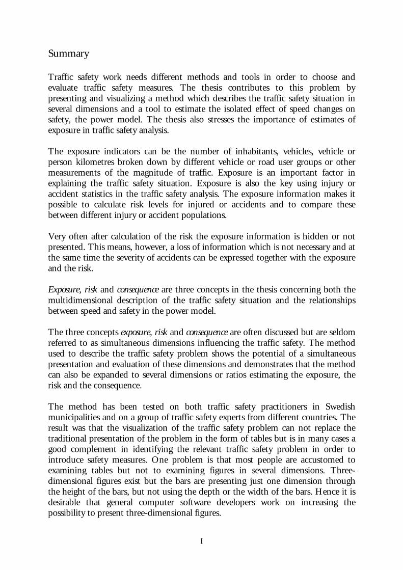
Appendix 2 QUESTIONNAIRE – Judgement of a traffic safety problem v Definitions used: Accident rate = Number of accidents per million vehicle kilometres Injury rate = All injured (incl. fatalities) per million vehicle kilometres Fatality rate = Number of fatalities per million (billion) vehicle kilometres Accident risk = Number of accidents per million person kilometres Injury risk = Number of all injured (incl. fatalities) per million person kilometres Fatality risk = Number of fatalities per million (billion) person kilometres Vehicle accident rate = Number of vehicles in accidents per million vehicle kilometres Driver accident risk = Number of accident involved drivers per million driver kilometres “Vehicle accident rate = Driver accident risk” (as vehicle kilometres is the same as driver kilometres) Fatal consequence = Number of fatalities per fatal accident Injury consequence = Number of injured (incl. fatalities) per injury accident Fatal accident consequence = Number of fatal accidents per injury accident

I

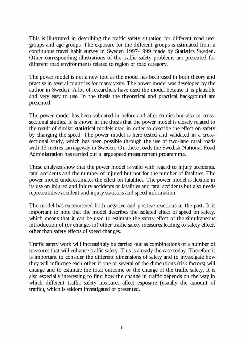
Summary Traffic safety work needs different methods and tools in order to choose and evaluate traffic safety measures. The thesis contributes to this problem by presenting and visualizing a method which describes the traffic safety situation in several dimensions and a tool to estimate the isolated effect of speed changes on safety, the power model. The thesis also stresses the importance of estimates of exposure in traffic safety analysis. The exposure indicators can be the number of inhabitants, vehicles, vehicle or person kilometres broken down by different vehicle or road user groups or other measurements of the magnitude of traffic. Exposure is an important factor in explaining the traffic safety situation. Exposure is also the key using injury or accident statistics in the traffic safety analysis. The exposure information makes it possible to calculate risk levels for injured or accidents and to compare these between different injury or accident populations. Very often after calculation of the risk the exposure information is hidden or not presented. This means, however, a loss of information which is not necessary and at the same time the severity of accidents can be expressed together with the exposure and the risk. Exposure, risk and consequence are three concepts in the thesis concerning both the multidimensional description of the traffic safety situation and the relationships between speed and safety in the power model. The three concepts exposure, risk and consequence are often discussed but are seldom referred to as simultaneous dimensions influencing the traffic safety. The method used to describe the traffic safety problem shows the potential of a simultaneous presentation and evaluation of these dimensions and demonstrates that the method can also be expanded to several dimensions or ratios estimating the exposure, the risk and the consequence. The method has been tested on both traffic safety practitioners in Swedish municipalities and on a group of traffic safety experts from different countries. The result was that the visualization of the traffic safety problem can not replace the traditional presentation of the problem in the form of tables but is in many cases a good complement in identifying the relevant traffic safety problem in order to introduce safety measures. One problem is that most people are accustomed to examining tables but not to examining figures in several dimensions. Three-dimensional figures exist but the bars are presenting just one dimension through the height of the bars, but not using the depth or the width of the bars. Hence it is desirable that general computer software developers work on increasing the possibility to present three-dimensional figures.

II

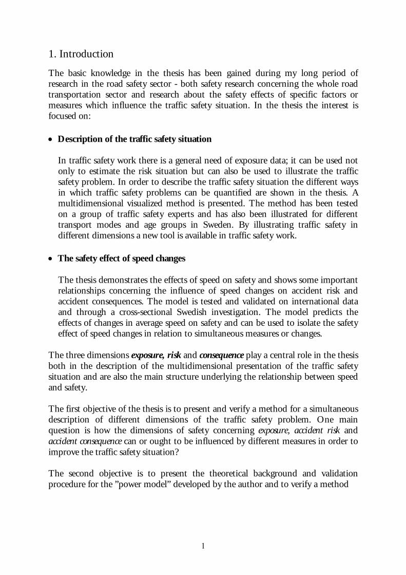
This is illustrated in describing the traffic safety situation for different road user groups and age groups. The exposure for the different groups is estimated from a continuous travel habit survey in Sweden 1997-1999 made by Statistics Sweden. Other corresponding illustrations of the traffic safety problems are presented for different road environments related to region or road category. The power model is not a new tool as the model has been used in both theory and practise in several countries for many years. The power model was developed by the author in Sweden. A lot of researchers have used the model because it is plausible and very easy to use. In the thesis the theoretical and practical background are presented. The power model has been validated in before and after studies but also in cross-sectional studies. It is shown in the thesis that the power model is closely related to the result of similar statistical models used in order to describe the effect on safety by changing the speed. The power model is here tested and validated in a cross-sectional study, which has been possible through the use of two-lane rural roads with 13 metres carriageway in Sweden. On these roads the Swedish National Road Administration has carried out a large speed measurement programme. These analyses show that the power model is valid with regard to injury accidents, fatal accidents and the number of injured but not for the number of fatalities. The power model underestimates the effect on fatalities. The power model is flexible in its use on injured and injury accidents or fatalities and fatal accidents but also needs representative accident and injury statistics and speed information. The model has encountered both negative and positive reactions in the past. It is important to note that the model describes the isolated effect of speed on safety, which means that it can be used to estimate the safety effect of the simultaneous introduction of (or changes in) other traffic safety measures leading to safety effects other than safety effects of speed changes. Traffic safety work will increasingly be carried out as combinations of a number of measures that will enhance traffic safety. This is already the case today. Therefore it is important to consider the different dimensions of safety and to investigate how they will influence each other if one or several of the dimensions (risk factors) will change and to estimate the total outcome or the change of the traffic safety. It is also especially interesting to find how the change in traffic depends on the way in which different traffic safety measures affect exposure (usually the amount of traffic), which is seldom investigated or presented.

1

1. Introduction

The basic knowledge in the thesis has been gained during my long period of research in the road safety sector - both safety research concerning the whole road transportation sector and research about the safety effects of specific factors or measures which influence the traffic safety situation. In the thesis the interest is focused on: • Description of the traffic safety situation In traffic safety work there is a general need of exposure data; it can be used not

only to estimate the risk situation but can also be used to illustrate the traffic safety problem. In order to describe the traffic safety situation the different ways in which traffic safety problems can be quantified are shown in the thesis. A multidimensional visualized method is presented. The method has been tested on a group of traffic safety experts and has also been illustrated for different transport modes and age groups in Sweden. By illustrating traffic safety in different dimensions a new tool is available in traffic safety work.

• The safety effect of speed changes

The thesis demonstrates the effects of speed on safety and shows some important relationships concerning the influence of speed changes on accident risk and accident consequences. The model is tested and validated on international data and through a cross-sectional Swedish investigation. The model predicts the effects of changes in average speed on safety and can be used to isolate the safety effect of speed changes in relation to simultaneous measures or changes.

The three dimensions exposure, risk and consequence play a central role in the thesis both in the description of the multidimensional presentation of the traffic safety situation and are also the main structure underlying the relationship between speed and safety. The first objective of the thesis is to present and verify a method for a simultaneous description of different dimensions of the traffic safety problem. One main question is how the dimensions of safety concerning exposure, accident risk and accident consequence can or ought to be influenced by different measures in order to improve the traffic safety situation? The second objective is to present the theoretical background and validation procedure for the ”power model” developed by the author and to verify a method

2

to assess the safety effect due to speed regulation measures. In order to identify relevant measures in traffic safety work speed measures are important (Allsop 1995). Speed is one of the main safety factors and influences both accident risk and accident consequence.

2. Description of the traffic accident problem

2.1 Background Almost all traffic or transportation in the road system has a transport purpose to move goods or people from one place to another. But in addition to this purpose of transport there are other considerations. One such considerations is to avoid situations resulting in accidents and especially accidents, which can result in injuries and in severe cases in fatalities. The number of accidents is a serious problem in society because they result in too many injured persons and fatalities. These injuries create a lot of negative consequences both for those injured and for others and put demands on resources from society.

The road transport system is normally described by its three main components and their subgroups. • The driver/road users - transportation mode, age, gender .. • The vehicles - different types of vehicles, vehicle speed.... • The roads - streets, motorways, road width, number of lanes, speed limit,

weather and light conditions…

Safety in the transport system depends on interactions between and within the three components and interactions between different drivers/road users. The interactions can be related to different risk factors, which increase or decrease the probability of an accident. In each situation in traffic it is possible that an accident may take place. An accident occurs due to some breakdown in the interaction between and within the components in the situation. The road safety situation is often described in different dimensions concerning safety in relation to the different components in traffic or combinations of the components. One main reason for this is that measures to reduce the influence of the risk factors in traffic are related to the components. As the accidents are rare and random events they can be described as a statistic phenomenon and experience shows that the Poisson distribution or closely related statistical distributions can approximate the accident distribution. The Poisson distribution has some properties, which are important

3

- The variance is the same as the expected value - The sum of the outcomes of Poisson distributed variables with parameter λi is

Poisson distributed with parameter Σλi. If the expected number of accidents in a road network during a time period is λ the probability of m accidents is

P(x=m) =!m

em λλ −

(2.1)

The expected number of accidents in a time period i.e. λ can be called risk. The risk factors influence not only the accident risk but also the consequence. The accident consequence differs a lot depending on accident type, speed, road user category involved etc. The number of situations or the magnitude of traffic is called the exposure. In order to estimate risk, exposure data is needed. Risk is usually defined as a ratio between the number of accidents or casualties and exposure. Using the accident information, we can describe the accident consequences in number of injuries and fatalities or in accident costs, hospital days etc.. The injury consequence is affected by the amount of violence caused to the human body. The forces are caused by the masses and accelerations involved. The accelerations are due to the speeds of the colliding objects. The safety situation can then be presented in terms of accidents, injured or fatalities, corresponding risks and exposures for different combinations of inhabitant groups, vehicle groups and road groups. The background theory of the traffic safety problem is that the change in the traffic safety problem is not only directly proportional to the change in traffic exposure but is also influenced by simultaneously changes in accident risk and accident consequence. This shall not be confused with the relationship between accident risk and traffic flow. Traffic flow can be regarded as another dimension of vehicle exposure. Of course a change in traffic flow can be the factor behind the change in accident risk or accident consequence (Ekman 1996). Different measures or factors influence the accident risk and accident consequences in the transport system at the same time as the change in traffic exposure occurs. The accident risk or the accident consequence can of course change even if the exposure is unchanged.

4

It is seldom possible to answer the question “Why do accidents happen?” On the other hand it is possible to identify, through empirical accident investigations, the different risk factors and the way they influence the risk level. For every defined time period and part of the transport system the expected number of injured persons or accidents can be estimated from the known risk factors, the consequence and the exposure. A description in one dimension of the traffic safety situation in terms of the number of fatalities, injuries or accidents normally gives no indication of the type of measures which are most efficient in reducing the observed number of fatalities, injuries or accidents. It is useful to classify measures according to the effect of the measure. Will the measure influence the exposure, the accident risk or the accident consequence? These three dimensions have been presented by many authors, who however, have not really used them in practical work (Elvik et al 1997, COST 329 1998). The method is further illustrated in the thesis by the traffic safety situation of different transport modes and road user age groups in Sweden in 1997-1999. A corresponding theory is behind the DRAG-model (modèle de la Demande Routière des Accidents et de leur Gravité), which is based on time-series of indicators. The elasticity of the indicator in relation to corresponding monthly values of fatal or injury accidents estimate the effect on safety by the indicator. The exposure is the principal component of the method. The model includes both the exposure part and the risk part, but in the parameter estimation phase both parts are estimated at the same time. (Gaudry & Lassarre 2000).

5

2.2 Hypotheses on traffic safety description The following hypotheses are stated. By illustrating the traffic safety situation simultaneously in several dimensions a method is developed which - simplifies the understanding of the traffic safety problem - helps in identifying relevant safety measures - makes it easier to evaluate the safety effect of measures There is a multiplicative dimensional relationship Risk Consequence

E(Injured) = Exposure*

AccidentsInjured

ExposureAccidents * (2.2)

or

E(Fatalities) = Exposure*

Injured

FatalitiesExposureInjured * (2.3)

Before the presentation of the three-dimensional method the need and use of accident and exposure data is presented in order to estimate the risk and the consequence dimension.

6

3. Accident data and exposure data to describe the traffic safety problem Generally, there are three main information sources used in traffic safety analysis: • Accident and/or injury data • Exposure data • Public records The public records can refer to the number of registered vehicles, the number of driving licences, population etc.. Together with accident and/or injury data collected for the same category and time period, calculations or estimates of risk situations can be made. Normally, there is no problem in calculating risks in relation to national accident registration systems except for trip data. Exposure data is normally collected for road users, vehicles and road groups and estimated for specified time periods (and trip purposes). Accident information is the basis in describing the magnitude of different traffic safety problems. However, in order to compare and rank different traffic safety problems, the key information is the description of the magnitude of the activities behind different traffic safety problems, the exposure. This chapter presents available accident, injury and exposure information in order to present comparable relevant descriptions of different traffic safety problems. 3.1 Accident registration As regards traffic accident and/or injury data, in most countries accidents are registered by the police. In addition to the official accident registration, there are a number of other sources (Thulin 1987): - Insurance company data: only insured vehicles in road accidents - Hospital data: only persons (patients) injured in road accidents who are

hospitalised - Accident involvement survey data and other self-reporting data. All sources have their advantages and disadvantages. It has to be stressed that these alternative databases are usually set up for different purposes than traffic safety. When the road users are asked about their involvement in traffic accidents they describe many more accidents with minor injuries than can be found from the other sources (Roosmark & Fräki 1970).

7

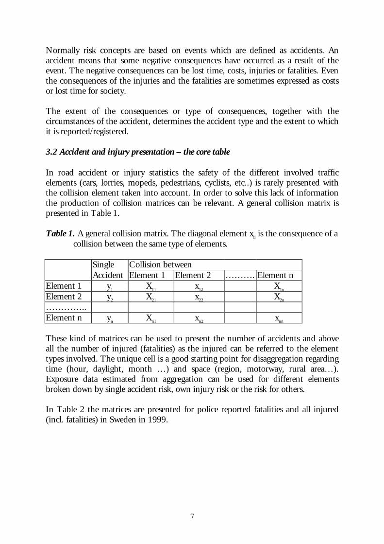
Normally risk concepts are based on events which are defined as accidents. An accident means that some negative consequences have occurred as a result of the event. The negative consequences can be lost time, costs, injuries or fatalities. Even the consequences of the injuries and the fatalities are sometimes expressed as costs or lost time for society. The extent of the consequences or type of consequences, together with the circumstances of the accident, determines the accident type and the extent to which it is reported/registered. 3.2 Accident and injury presentation – the core table In road accident or injury statistics the safety of the different involved traffic elements (cars, lorries, mopeds, pedestrians, cyclists, etc..) is rarely presented with the collision element taken into account. In order to solve this lack of information the production of collision matrices can be relevant. A general collision matrix is presented in Table 1. Table 1. A general collision matrix. The diagonal element xii is the consequence of a

collision between the same type of elements. Single Collision between Accident Element 1 Element 2 ………. Element n Element 1 y1 X11 x12 X1n

Element 2 y2 X21 x22 X2n

………….. Element n yn Xn1 xn2 xnn

These kind of matrices can be used to present the number of accidents and above all the number of injured (fatalities) as the injured can be referred to the element types involved. The unique cell is a good starting point for disaggregation regarding time (hour, daylight, month …) and space (region, motorway, rural area…). Exposure data estimated from aggregation can be used for different elements broken down by single accident risk, own injury risk or the risk for others. In Table 2 the matrices are presented for police reported fatalities and all injured (incl. fatalities) in Sweden in 1999.

8

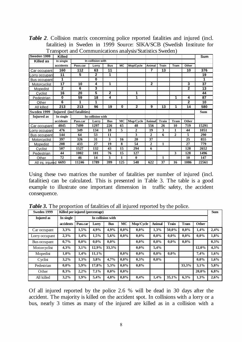
Table 2. Collision matrix concerning police reported fatalities and injured (incl.

fatalities) in Sweden in 1999 Source: SIKA/SCB (Swedish Institute for Transport and Communications analysis/Statistics Sweden)

Sweden 1999 Killed SumKilled as In single In collision with

accidents Pass.car Lorry Bus MC Mop/Cycle Animal Train Tram Other Car occupant 160 112 63 11 7 13 10 376

Lorry occupant 11 5 2 1 19Bus occupant 1 0 1Motorcyclist 17 10 4 1 2 3 37

Mopedist 2 6 3 2 13Cyclist 16 20 5 2 1 44

Pedestrian 0 59 18 4 1 1 4 87Other 6 1 1 2 10

All killed 213 213 96 19 0 2 9 13 1 14 580 Sweden 1999 Injured (incl fatalities)

SumInjured as In single In collision with

accidents Pass.car Lorry Bus MC Mop/Cycle Animal Train Tram Other Car occupant 4845 7499 1297 226 65 48 556 26 10 719 15291

Lorry occupant 476 349 134 18 5 2 19 3 1 44 1051Bus occupant 144 64 53 11 3 2 6 2 5 290Motorcyclist 397 326 31 3 16 20 37 25 855

Mopedist 208 433 27 19 8 54 2 1 27 779Cyclist 507 1527 132 43 15 294 6 128 2652

Pedestrian 44 1002 101 76 15 127 3 128 1496Other 72 46 14 3 1 0 1 10 147

All inj. injured 6693 11246 1789 399 125 548 622 37 16 1086 22561 Using these two matrices the number of fatalities per number of injured (incl. fatalities) can be calculated. This is presented in Table 3. The table is a good example to illustrate one important dimension in traffic safety, the accident consequence. Table 3. The proportion of fatalities of all injured reported by the police.

Sweden 1999 Killed per injured (percentage) Sum

Injured as In single In collision with

accidents Pass.car Lorry Bus MC Mop/Cycle Animal Train Tram Other

Car occupant 3,3% 1,5% 4,9% 4,9% 0,0% 0,0% 1,3% 50,0% 0,0% 1,4% 2,4%

Lorry occupant 2,3% 1,4% 1,5% 5,6% 0,0% 0,0% 0,0% 0,0% 0,0% 0,0% 1,8%

Bus occupant 0,7% 0,0% 0,0% 0,0% 0,0% 0,0% 0,0% 0,0% 0,3%

Motorcyclist 4,3% 3,1% 12,9% 33,3% 0,0% 5,4% 12,0% 4,3%

Mopedist 1,0% 1,4% 11,1% 0,0% 0,0% 0,0% 0,0% 7,4% 1,6%

Cyclist 3,2% 1,3% 3,8% 4,7% 0,0% 0,3% 0,0% 0,0% 1,6%

Pedestrian 0,0% 5,9% 17,8% 5,3% 0,0% 0,8% 33,3% 3,1% 5,8%

Other 8,3% 2,2% 7,1% 0,0% 0,0% 20,0% 6,8%

All killed 3,2% 1,9% 5,4% 4,8% 0,0% 0,4% 1,4% 35,1% 6,3% 1,3% 2,6%

Of all injured reported by the police 2.6 % will be dead in 30 days after the accident. The majority is killed on the accident spot. In collisions with a lorry or a bus, nearly 3 times as many of the injured are killed as in a collision with a

9

passenger car. This relation between passenger cars and lorry/bus is about the same for all road users. Collisions with trains and trams are disasters for car occupants and pedestrians respectively. One problem above is that a high percentage concerning fatalities among the injured to some extent depends on the reporting system, but also on a random fluctuation as the numbers of fatalities and injured are sometimes small. The above matrices are the basic ones needed for accident, injury or fatality statistics. Very few accident registration systems use this kind of registration or presentation. What is interesting with these kinds of matrices is that exposure can be used directly in regard to both the rows and the columns. The rows can be distributed over single accidents and collisions. One problem is that collisions with more than two traffic elements involved ought to be solved. Fortunately the number of such collisions is quite small. The concept of induced exposure has been developed on the basis of accident statistics and collision tables such as those presented above (Wass 1977). The problem with induced exposure is that at the same time the risk is also an induced one, which means two indirect estimated values to interpret. Only the product of the induced exposure and the induced risk is a “direct” safety indicator, i.e. the number of accidents for the group of interest. The matrices can be disaggregated to road type, accident type, gender, age groups, space and/or time. The disaggregation ought to coincide with the existing exposure measurement. 3.3 Exposure data and risk estimates

Even if the accident (injury) reporting system is the basic information source, the exposure data is necessary for meaningful road safety analysis. Exposure data is normally not collected for safety purposes but for different (economic) planning procedures in society. The main purpose is for road planning. The concept of risk is a relation (ratio) between accidents or casualties and some indicator describing exposure (the units or the magnitude of the activity in which the accidents occurred) and can be referred to as accident or casualty risks. The exposure can be described in different ways, as number of involved units, distance travelled, time spent in traffic, number of trips or traffic situations related to different accident types (Nilsson 1978).

10

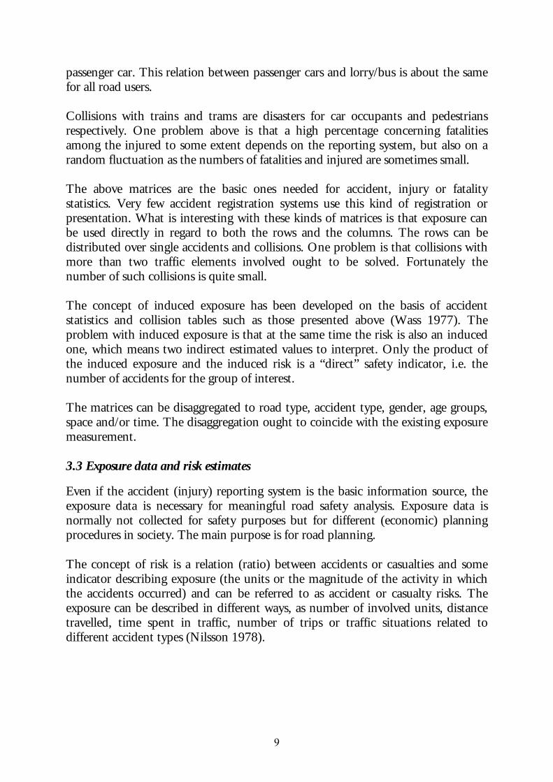
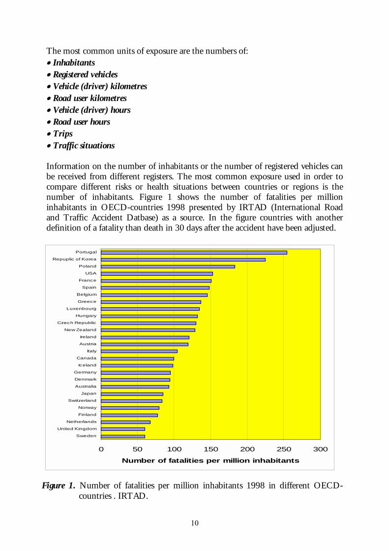
The most common units of exposure are the numbers of: • Inhabitants • Registered vehicles • Vehicle (driver) kilometres • Road user kilometres • Vehicle (driver) hours • Road user hours • Trips • Traffic situations Information on the number of inhabitants or the number of registered vehicles can be received from different registers. The most common exposure used in order to compare different risks or health situations between countries or regions is the number of inhabitants. Figure 1 shows the number of fatalities per million inhabitants in OECD-countries 1998 presented by IRTAD (International Road and Traffic Accident Datbase) as a source. In the figure countries with another definition of a fatality than death in 30 days after the accident have been adjusted.

0 50 100 150 200 250 300

Sweden

United Kingdom

Netherlands

Finland

Norway

Switzerland

Japan

Australia

Denmark

Germany

Iceland

Canada

Italy

Austria

Ireland

New Zealand

Czech Republic

Hungary

Luxenbourg

Greece

Belgium

Spain

France

USA

Poland

Repuplic of Korea

Portugal

Number of fatalities per million inhabitants

Figure 1. Number of fatalities per million inhabitants 1998 in different OECD-

countries . IRTAD.

11

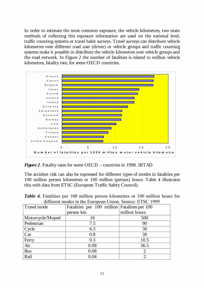
In order to estimate the most common exposure, the vehicle kilometres, two main methods of collecting this exposure information are used on the national level, traffic counting systems or travel habit surveys. Travel surveys can distribute vehicle kilometres over different road user (driver) or vehicle groups and traffic counting systems make it possible to distribute the vehicle kilometres over vehicle groups and the road network. In Figure 2 the number of fatalities is related to million vehicle kilometres, fatality rate, for some OECD countries.

Figure 2. Fatality rates for some OECD – countries in 1998. IRTAD

The accident risk can also be expressed for different types of modes in fatalities per 100 million person kilometres or 100 million (person) hours. Table 4 illustrates this with data from ETSC (European Traffic Safety Council). Table 4. Fatalities per 100 million person kilometres or 100 million hours for

different modes in the European Union. Source: ETSC 1999 Travel mode Fatalities per 100 million

person km Fatalities per 100 million hours

Motorcycle/Moped 16 500 Pedestrian 7.5 90 Cycle 6.3 30 Car 0.8 30 Ferry 0.3 10.5 Air 0.08 36.5 Bus 0.08 2 Rail 0.04 2

0 5 1 0 1 5 2 0

U n i t e d K i n g d o m

S w e d e n

F i n l a n d

N e t h e r l a n d s

U S A

N o r w a y

D e n m a r k

S w i t z e r l a n d

G e r m a n y

I r e l a n d

I c e l a n d

A u s t r i a

J a p a n

B e l g i u m

F r a n c e

G r e e c e

N u m b e r o f f a t a l i t i e s p e r 1 0 0 0 m i l l i o n m o t o r v e h i c l e k i l o m e t r e

12

Motorcycle/Moped is the most dangerous transport mode and rail the safest. The above examples of risk presentations are one-dimensional presentations. How about the number of fatalities and the magnitude of the exposure? The way these dimensions and other dimensions can be simultaneously visualized is demonstrated in the next chapter.

13

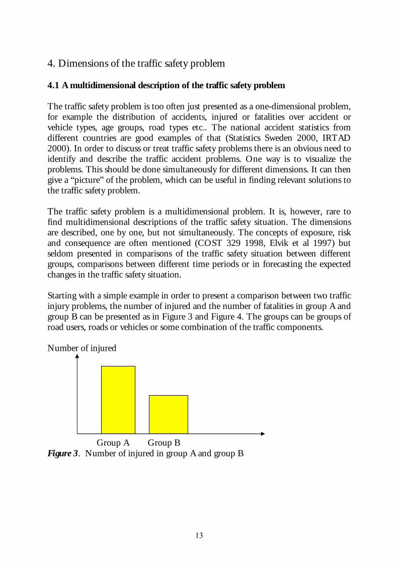
4. Dimensions of the traffic safety problem 4.1 A multidimensional description of the traffic safety problem The traffic safety problem is too often just presented as a one-dimensional problem, for example the distribution of accidents, injured or fatalities over accident or vehicle types, age groups, road types etc.. The national accident statistics from different countries are good examples of that (Statistics Sweden 2000, IRTAD 2000). In order to discuss or treat traffic safety problems there is an obvious need to identify and describe the traffic accident problems. One way is to visualize the problems. This should be done simultaneously for different dimensions. It can then give a “picture” of the problem, which can be useful in finding relevant solutions to the traffic safety problem. The traffic safety problem is a multidimensional problem. It is, however, rare to find multidimensional descriptions of the traffic safety situation. The dimensions are described, one by one, but not simultaneously. The concepts of exposure, risk and consequence are often mentioned (COST 329 1998, Elvik et al 1997) but seldom presented in comparisons of the traffic safety situation between different groups, comparisons between different time periods or in forecasting the expected changes in the traffic safety situation. Starting with a simple example in order to present a comparison between two traffic injury problems, the number of injured and the number of fatalities in group A and group B can be presented as in Figure 3 and Figure 4. The groups can be groups of road users, roads or vehicles or some combination of the traffic components. Number of injured Group A Group B Figure 3. Number of injured in group A and group B

14

Number of fatalities Group A Group B Figure 4. Number of fatalities in group A and in group B Group A has more injured than group B. As regards fatalities the two groups are identical. Only one dimension at a time has been used. One main question is whether the entities in group A and B have different risks of injuries or fatalities. Now it is necessary to define some exposure information, which can be used in describing the possible risk difference. The risk concept, the occurrence of an injury or accident involvement of a vehicle or road user in relation to exposure, can be generalised by a risk indicator. How is it possible to describe the risk? Is it valid for the transport system, for the activity, for those involved or for someone else? One answer is that the risk indicator or measurement shall be able to identify the effect of measures or other changes. Every risk indicator is just one dimension (or one description) of the problem. The traffic safety problem to be solved has several dimensions – the measures to take are many and directed at different parts or components of the transport system. The safety problem or measures taken ought to be described with a relevant risk indicator for the case in question.

rDenominatoNumerator

ExposureInjured)Accidents(indicator Risk == (4.1)

The choice of exposure or the available indicator of exposure creates the denominator in the risk indicator such as population, vehicle or person kilometres, time or trips etc.. The investigation time is decided by the accident period or the period or space for the available exposure measurement. The risk situation can be described for different subgroups depending on the exposure and whether the numerator (accidents/injured) and the denominator (exposure) can be disaggregated in the same way.

15

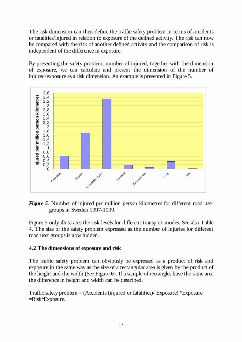
The risk dimension can then define the traffic safety problem in terms of accidents or fatalities/injured in relation to exposure of the defined activity. The risk can now be compared with the risk of another defined activity and the comparison of risk is independent of the difference in exposure. By presenting the safety problem, number of injured, together with the dimension of exposure, we can calculate and present the dimension of the number of injured/exposure as a risk dimension. An example is presented in Figure 5.

00,20,40,60,8

11,21,41,61,8

22,22,42,62,8

33,23,43,6

Pedes

trian

Bicycle

Moped

/Moto

rcycle

Car dri

ver

Car pa

ssen

ger

Lorry

Bus

Inju

red

per m

illio

n pe

rson

kilo

met

res

Figure 5. Number of injured per million person kilometres for different road user

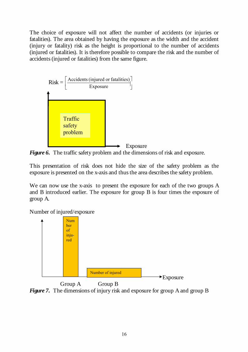
groups in Sweden 1997-1999. Figure 5 only illustrates the risk levels for different transport modes. See also Table 4. The size of the safety problem expressed as the number of injuries for different road user groups is now hidden. 4.2 The dimensions of exposure and risk The traffic safety problem can obviously be expressed as a product of risk and exposure in the same way as the size of a rectangular area is given by the product of the height and the width (See Figure 6). If a sample of rectangles have the same area the difference in height and width can be described. Traffic safety problem = (Accidents (injured or fatalities)/ Exposure) *Exposure =Risk*Exposure.

16

The choice of exposure will not affect the number of accidents (or injuries or fatalities). The area obtained by having the exposure as the width and the accident (injury or fatality) risk as the height is proportional to the number of accidents (injured or fatalities). It is therefore possible to compare the risk and the number of accidents (injured or fatalities) from the same figure.

Risk =

Exposure

)fatalitiesor (injured Accidents

Exposure Figure 6. The traffic safety problem and the dimensions of risk and exposure. This presentation of risk does not hide the size of the safety problem as the exposure is presented on the x-axis and thus the area describes the safety problem. We can now use the x-axis to present the exposure for each of the two groups A and B introduced earlier. The exposure for group B is four times the exposure of group A. Number of injured/exposure Exposure Group A Group B Figure 7. The dimensions of injury risk and exposure for group A and group B

Traffic safety problem

Number of inju-red

Number of injured

17

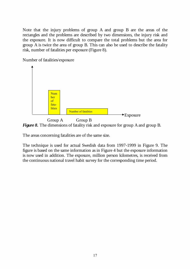
Note that the injury problems of group A and group B are the areas of the rectangles and the problems are described by two dimensions, the injury risk and the exposure. It is now difficult to compare the total problems but the area for group A is twice the area of group B. This can also be used to describe the fatality risk, number of fatalities per exposure (Figure 8). Number of fatalities/exposure Exposure Group A Group B Figure 8. The dimensions of fatality risk and exposure for group A and group B. The areas concerning fatalities are of the same size. The technique is used for actual Swedish data from 1997-1999 in Figure 9. The figure is based on the same information as in Figure 4 but the exposure information is now used in addition. The exposure, million person kilometres, is received from the continuous national travel habit survey for the corresponding time period.

Number of fata-lities

Number of fatalities

18

00,20,40,60,8

11,21,41,61,8

22,22,42,62,8

33,23,43,6

0 10000 20000 30000 40000 50000 60000 70000 80000 90000 100000 110000

Ex posure

Inju

red

per

mill

ion

pers

on k

ilom

etre

s

Pede

stria

nB

icyc

leMoped/Motorcycle

C ar driver C ar passenger

Lorry

Bus

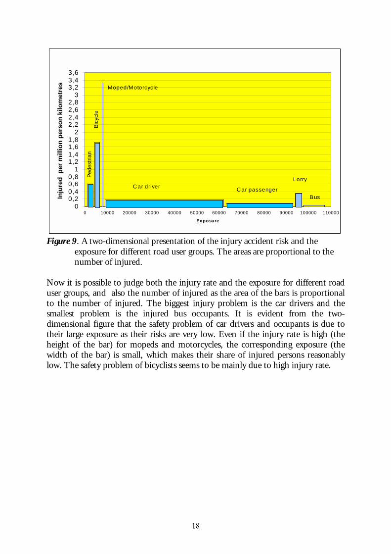
Figure 9. A two-dimensional presentation of the injury accident risk and the

exposure for different road user groups. The areas are proportional to the number of injured.

Now it is possible to judge both the injury rate and the exposure for different road user groups, and also the number of injured as the area of the bars is proportional to the number of injured. The biggest injury problem is the car drivers and the smallest problem is the injured bus occupants. It is evident from the two-dimensional figure that the safety problem of car drivers and occupants is due to their large exposure as their risks are very low. Even if the injury rate is high (the height of the bar) for mopeds and motorcycles, the corresponding exposure (the width of the bar) is small, which makes their share of injured persons reasonably low. The safety problem of bicyclists seems to be mainly due to high injury rate.

19

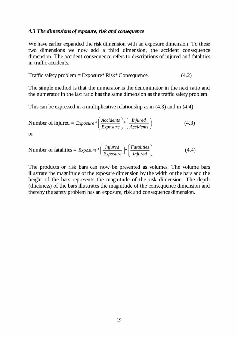
4.3 The dimensions of exposure, risk and consequence We have earlier expanded the risk dimension with an exposure dimension. To these two dimensions we now add a third dimension, the accident consequence dimension. The accident consequence refers to descriptions of injured and fatalities in traffic accidents. Traffic safety problem = Exposure* Risk* Consequence. (4.2) The simple method is that the numerator is the denominator in the next ratio and the numerator in the last ratio has the same dimension as the traffic safety problem. This can be expressed in a multiplicative relationship as in (4.3) and in (4.4)

Number of injured =

AccidentsInjured

ExposureAccidentsExposure ** (4.3)

or

Number of fatalities =

Injured

FatalitiesExposureInjuredExposure ** (4.4)

The products or risk bars can now be presented as volumes. The volume bars illustrate the magnitude of the exposure dimension by the width of the bars and the height of the bars represents the magnitude of the risk dimension. The depth (thickness) of the bars illustrates the magnitude of the consequence dimension and thereby the safety problem has an exposure, risk and consequence dimension.

20

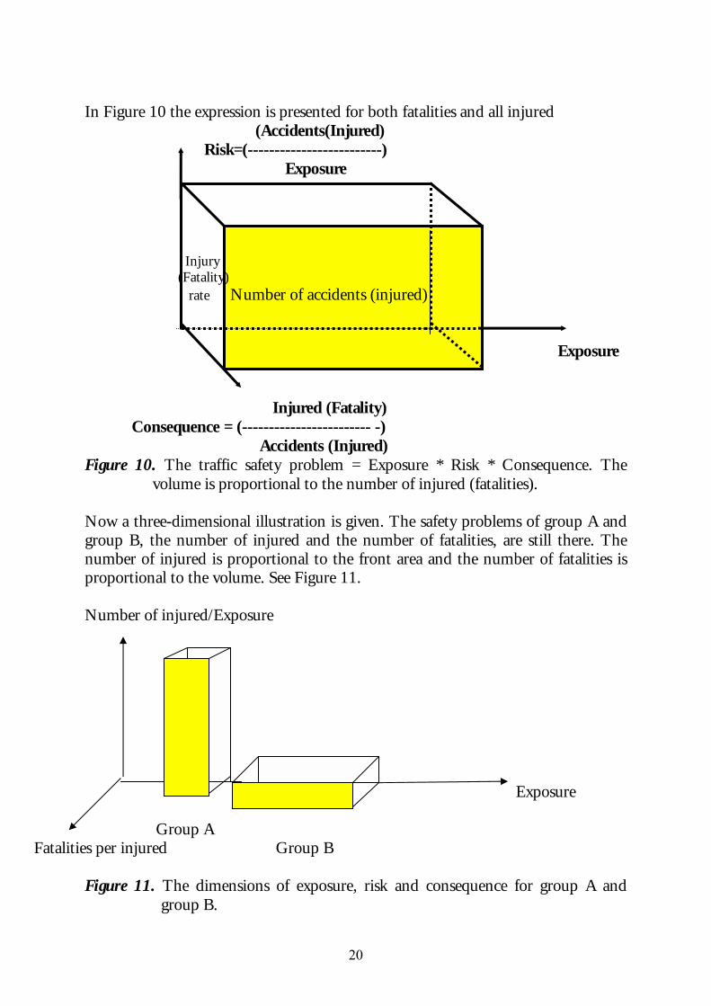
In Figure 10 the expression is presented for both fatalities and all injured (Accidents(Injured) Risk=(-------------------------) Exposure Injury (Fatality) rate Number of accidents (injured) Exposure Injured (Fatality) Consequence = (------------------------ -) Accidents (Injured) Figure 10. The traffic safety problem = Exposure * Risk * Consequence. The

volume is proportional to the number of injured (fatalities). Now a three-dimensional illustration is given. The safety problems of group A and group B, the number of injured and the number of fatalities, are still there. The number of injured is proportional to the front area and the number of fatalities is proportional to the volume. See Figure 11. Number of injured/Exposure

Exposure Group A

Fatalities per injured Group B

Figure 11. The dimensions of exposure, risk and consequence for group A and group B.

21

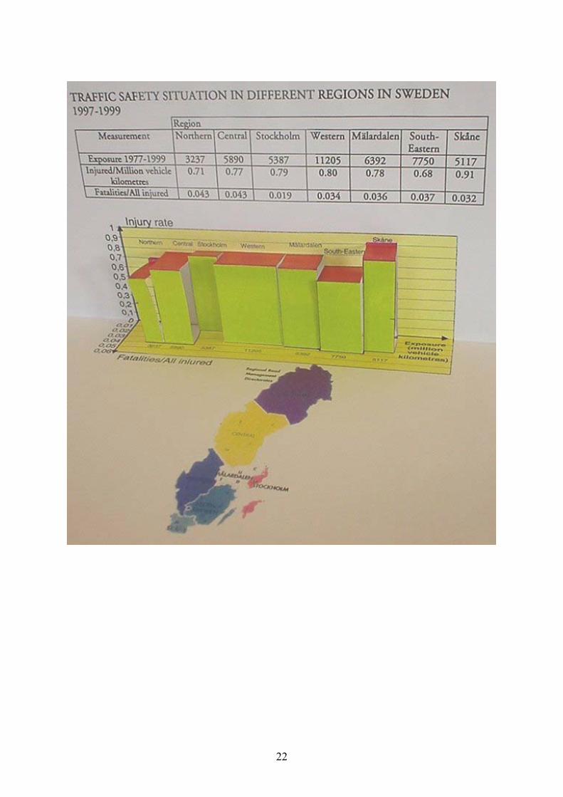
This kind of presentation has been used by the author (Nilsson 1981b, 1984a, Thulin et al 1994) and has been presented by others. (Holmberg & Hyden et al 1996). A practical problem is that normal software in computers has a limitation in presenting more than two dimensions in figures. The software used in this thesis is Mathematica Version 2. It is however possible to do it by hand, which is presented on the next page. In figure 12 the traffic safety situations in the seven Road Administration Regions in Sweden are presented concerning the number of police reported injured (incl. fatalities), number of fatalities and the estimated motor vehicle kilometres in 1999.

22

23

Figu

re 1

2. D

escr

ipti

on o

f the

traf

fic s

afet

y si

tuat

ion

on n

atio

nal r

oads

in th

e

.

Nat

iona

l Roa

d A

dmin

istr

atio

n R

egio

ns in

Sw

eden

in 1

999

24

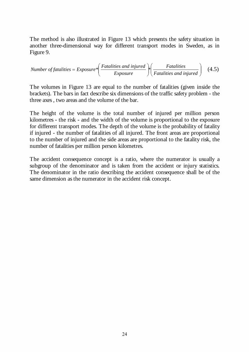
The method is also illustrated in Figure 13 which presents the safety situation in another three-dimensional way for different transport modes in Sweden, as in Figure 9.

=

ed and injurFatalitiesFatalities*

Exposureed and injurFatalitiesExposure*fatalitiesNumber of (4.5)

The volumes in Figure 13 are equal to the number of fatalities (given inside the brackets). The bars in fact describe six dimensions of the traffic safety problem - the three axes , two areas and the volume of the bar. The height of the volume is the total number of injured per million person kilometres - the risk - and the width of the volume is proportional to the exposure for different transport modes. The depth of the volume is the probability of fatality if injured - the number of fatalities of all injured. The front areas are proportional to the number of injured and the side areas are proportional to the fatality risk, the number of fatalities per million person kilometres. The accident consequence concept is a ratio, where the numerator is usually a subgroup of the denominator and is taken from the accident or injury statistics. The denominator in the ratio describing the accident consequence shall be of the same dimension as the numerator in the accident risk concept.

25

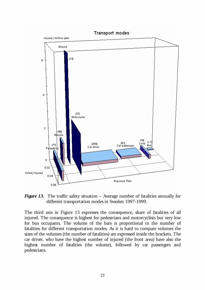
Figure 13. The traffic safety situation – Average number of fatalities annually for

different transportation modes in Sweden 1997-1999. The third axis in Figure 13 expresses the consequence, share of fatalities of all injured. The consequence is highest for pedestrians and motorcyclists but very low for bus occupants. The volume of the bars is proportional to the number of fatalities for different transportation modes. As it is hard to compare volumes the sizes of the volumes (the number of fatalities) are expressed inside the brackets. The car driver, who have the highest number of injured (the front area) have also the highest number of fatalities (the volume), followed by car passengers and pedestrians.

26

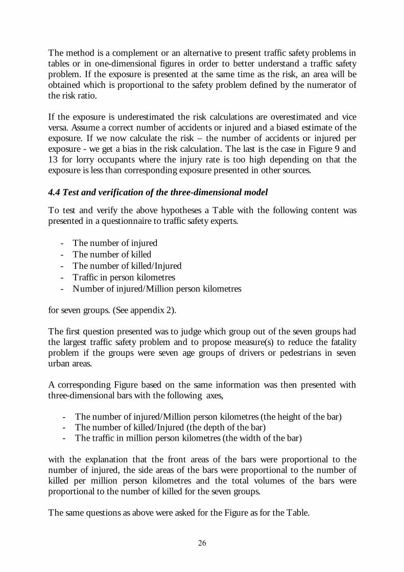
The method is a complement or an alternative to present traffic safety problems in tables or in one-dimensional figures in order to better understand a traffic safety problem. If the exposure is presented at the same time as the risk, an area will be obtained which is proportional to the safety problem defined by the numerator of the risk ratio. If the exposure is underestimated the risk calculations are overestimated and vice versa. Assume a correct number of accidents or injured and a biased estimate of the exposure. If we now calculate the risk – the number of accidents or injured per exposure - we get a bias in the risk calculation. The last is the case in Figure 9 and 13 for lorry occupants where the injury rate is too high depending on that the exposure is less than corresponding exposure presented in other sources. 4.4 Test and verification of the three-dimensional model To test and verify the above hypotheses a Table with the following content was presented in a questionnaire to traffic safety experts.

- The number of injured - The number of killed - The number of killed/Injured - Traffic in person kilometres - Number of injured/Million person kilometres

for seven groups. (See appendix 2). The first question presented was to judge which group out of the seven groups had the largest traffic safety problem and to propose measure(s) to reduce the fatality problem if the groups were seven age groups of drivers or pedestrians in seven urban areas. A corresponding Figure based on the same information was then presented with three-dimensional bars with the following axes, - The number of injured/Million person kilometres (the height of the bar) - The number of killed/Injured (the depth of the bar) - The traffic in million person kilometres (the width of the bar) with the explanation that the front areas of the bars were proportional to the number of injured, the side areas of the bars were proportional to the number of killed per million person kilometres and the total volumes of the bars were proportional to the number of killed for the seven groups. The same questions as above were asked for the Figure as for the Table.

27

The respondents were then asked if they

- Prefer the Table to the Figure - Prefer the Figure to the Table - Want both the Figure and the Table

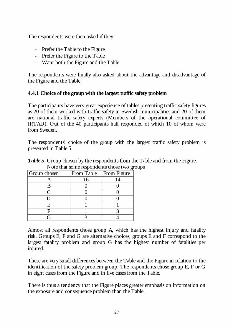
The respondents were finally also asked about the advantage and disadvantage of the Figure and the Table. 4.4.1 Choice of the group with the largest traffic safety problem The participants have very great experience of tables presenting traffic safety figures as 20 of them worked with traffic safety in Swedish municipalities and 20 of them are national traffic safety experts (Members of the operational committee of IRTAD). Out of the 40 participants half responded of which 10 of whom were from Sweden. The respondents' choice of the group with the largest traffic safety problem is presented in Table 5. Table 5. Group chosen by the respondents from the Table and from the Figure. Note that some respondents chose two groups Group chosen From Table From Figure

A 16 14 B 0 0 C 0 0 D 0 0 E 1 1 F 1 3 G 3 4

Almost all respondents chose group A, which has the highest injury and fatality risk. Groups E, F and G are alternative choices, groups E and F correspond to the largest fatality problem and group G has the highest number of fatalities per injured. There are very small differences between the Table and the Figure in relation to the identification of the safety problem group. The respondents chose group E, F or G in eight cases from the Figure and in five cases from the Table. There is thus a tendency that the Figure places greater emphasis on information on the exposure and consequence problem than the Table.

28

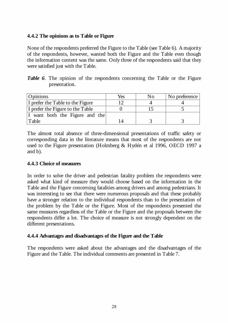
4.4.2 The opinions as to Table or Figure None of the respondents preferred the Figure to the Table (see Table 6). A majority of the respondents, however, wanted both the Figure and the Table even though the information content was the same. Only three of the respondents said that they were satisfied just with the Table. Table 6. The opinion of the respondents concerning the Table or the Figure

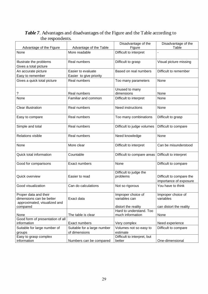
presentation. Opinions Yes No No preferenceI prefer the Table to the Figure 12 4 4 I prefer the Figure to the Table 0 15 5 I want both the Figure and the Table 14 3 3 The almost total absence of three-dimensional presentations of traffic safety or corresponding data in the literature means that most of the respondents are not used to the Figure presentation (Holmberg & Hydén et al 1996, OECD 1997 a and b). 4.4.3 Choice of measures In order to solve the driver and pedestrian fatality problem the respondents were asked what kind of measure they would choose based on the information in the Table and the Figure concerning fatalities among drivers and among pedestrians. It was interesting to see that there were numerous proposals and that these probably have a stronger relation to the individual respondents than to the presentation of the problem by the Table or the Figure. Most of the respondents presented the same measures regardless of the Table or the Figure and the proposals between the respondents differ a lot. The choice of measure is not strongly dependent on the different presentations. 4.4.4 Advantages and disadvantages of the Figure and the Table The respondents were asked about the advantages and the disadvantages of the Figure and the Table. The individual comments are presented in Table 7.

29

Table 7. Advantages and disadvantages of the Figure and the Table according to

the respondents.

Advantage of the Figure Advantage of the Table Disadvantage of the

Figure Disadvantage of the

Table None More readable Difficult to interpret - Illustrate the problems Real numbers Difficult to grasp Visual picture missing Gives a total picture An accurate picture Easier to evaluate Based on real numbers Difficult to remember Easy to remember Easier to give priority Gives a quick total picture Real numbers Too many parameters None

? Real numbers Unused to many dimensions None

None Familiar and common Difficult to interpret None Clear illustration Real numbers Need instructions None Easy to compare Real numbers Too many combinations Difficult to grasp Simple and total Real numbers Difficult to judge volumes Difficult to compare Relations visible Real numbers Need knowledge None None More clear Difficult to interpret Can be misunderstood Quick total information Countable Difficult to compare areas Difficult to interpret Good for comparisons Exact numbers None Difficult to compare

Quick overview Easier to read Difficult to judge the problems Difficult to compare the

importance of exposure Good visualization Can do calculations Not so rigorous You have to think Proper data and their dimensions can be better Exact data

Improper choice of variables can

Improper choice of variables

approximated, visualized and compared distort the reality can distort the reality

None The table is clear Hard to understand. Too much information None

Good form of presentation of all information Exact numbers Very complex Need experience Suitable for large number of Suitable for a large number Volumes not so easy to Difficult to compare groups of dimensions estimate Easy to grasp complex information Numbers can be compared

Difficult to interpret, but better One-dimensional

30

The advantages of the Table are obvious as numbers are regarded as exact values and the comparison of numbers and counting procedures can be carried out at once. Only three of the respondents were however satisfied with the Table alone and most of the respondents wished to have the Figure as a complement. The main reason was that the problem was made visible and that the total content of information could be grasped in a simple way (just by looking). The disadvantages of the Figure were its complexity and the need of instructions to interpret the Figure due to the limited experience the respondents had of this kind of Figures. Surprisingly most of the respondents stated that the Table had disadvantages and said that a Table is difficult to remember or needs experience to be interpreted. Six of the respondents had no problems with the Table but three of them also realised the benefits of the Figure. 4.4.5 Conclusions The first hypothesis, “the three-dimension method simplifies the understanding of the traffic safety problem”, can be confirmed and thereby verified. An increased experience of this kind of illustration will underline this. It is harder to verify the other two hypotheses that “the method increases the choice of relevant safety measures” and “the method makes it easier to evaluate the safety effect of measures”. The last hypothesis could not be verified with the survey used in this study. The choice of the traffic safety problem, however, may be slightly influenced by a Figure presentation as a complement to the Table. It was remarkable that the majority of the respondents evidently did not take into account the influence of the amount of exposure on the traffic safety problem when making their judgements.

31

4.5 The traffic safety situation of different transport modes and age groups in Sweden in 1997-1999

4.5.1 Data Since 1994 a continuous investigation about travel habits has been conducted by SCB/SIKA through telephone interviews (Statistics Sweden, 1999). Some of the results from this later investigation are presented below and will result in risk estimations. The results concern the period 1997-1999 and surface transportation. Table 8 presents the distribution of person kilometres for different transport modes and age groups.

Table 8. The distribution of annual person kilometres (millions) for different

modes and age groups in 1997-1999. Source: RES-SCB/SIKA

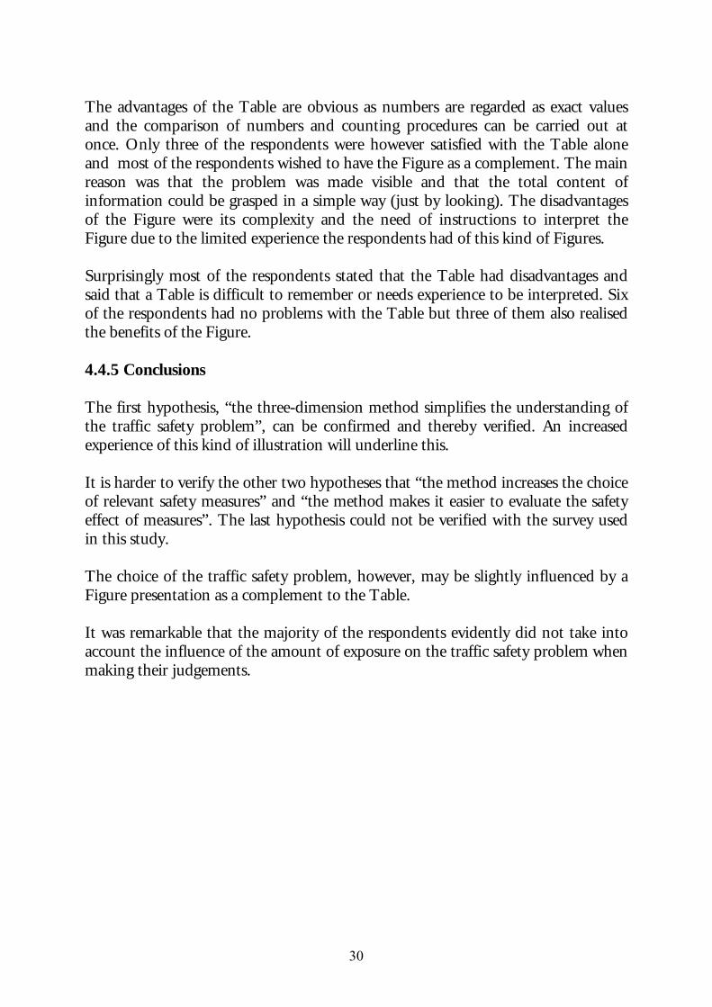
Age 0-14 15-17 18-24 25-34 35-44 45-54 55-64 65-74 75- Sum Pedestrian 244 148 280 388 300 397 297 273 128 2455 Cycle 337 183 250 325 301 348 215 113 43 2115 Moped 3 63 9 13 2 3 12 5 2 112 MC 0 13 36 168 93 26 13 0 0 349 Car driver 6 23 3631 11401 13057 12610 7686 3633 1021 53068 Car passenger 6979 1993 3130 4172 3680 3962 3031 2423 658 30028 Taxi 310 173 192 324 130 168 249 47 33 1626 Lorry 10 0 226 811 659 697 347 23 0 2773 Bus 981 1144 1794 988 1095 1464 1200 635 242 9543 Tractor 3 8 33 6 14 18 21 3 1 107 Rail traffic 355 463 1528 2772 905 1276 591 214 226 8330 Total 9228 4211 11108 21368 20236 20969 13663 7368 2653 110804 The dominating surface transport mode is the car and as a car driver. Bus and rail traffic person kilometres are of the same magnitude and each about 10 per cent of car use. Taxis are used by schoolchildren and by elderly persons who have some mobility problem. It is unclear to what extent taxi drivers are included. The use of rail traffic by young persons is to some extent dependent on the cheaper fares for students.

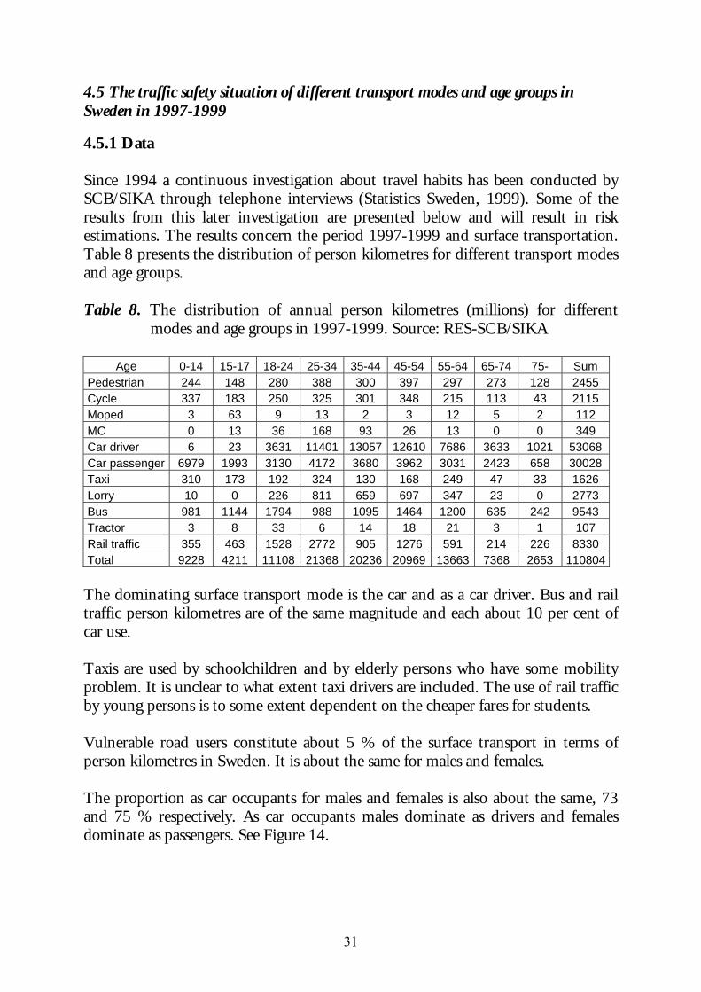
Vulnerable road users constitute about 5 % of the surface transport in terms of person kilometres in Sweden. It is about the same for males and females. The proportion as car occupants for males and females is also about the same, 73 and 75 % respectively. As car occupants males dominate as drivers and females dominate as passengers. See Figure 14.

32

M a le - L a n d t r a n s p o r t m o d e s

C a r d r ive r5 7 %

C a r p a s s e n g e r

1 6 %

T a xi1 %

L o r r y4 %

B u s7 %

R a i l1 1 %

T r a c to r0 , 1 5 %

M C0 , 4 1 %

M o p e d0 , 1 4 %

P e d e s tr ia n2 % C y c le

2 %

F e m a le -L a n d tra n s p o rt m o d e s

C ar passenger

42%

B us10%

C ar dr iver33%

P edestr ian3%Trac tor

0 ,02%Rail9%

C y c le2%

MC0,16%

Moped0,05%

Taxi1%

Lorry0,02%

Figure 14. The percentage distribution of person kilometres by different transport modes for males and females in Sweden, 1997-1999

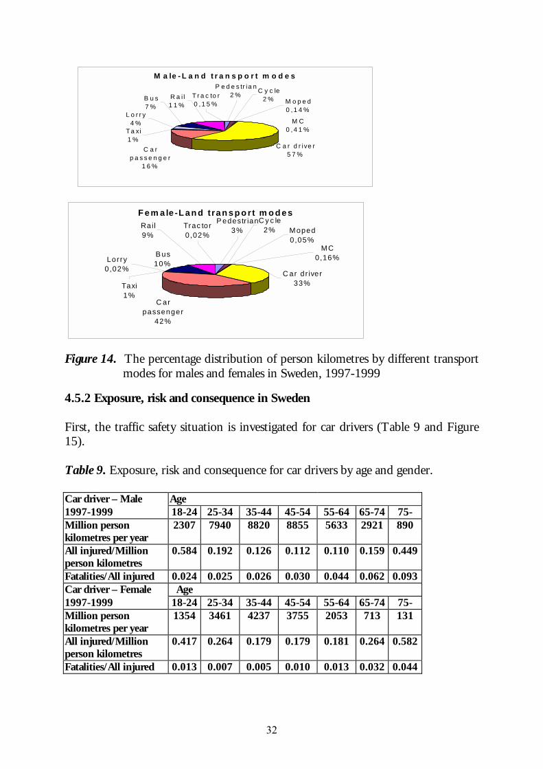
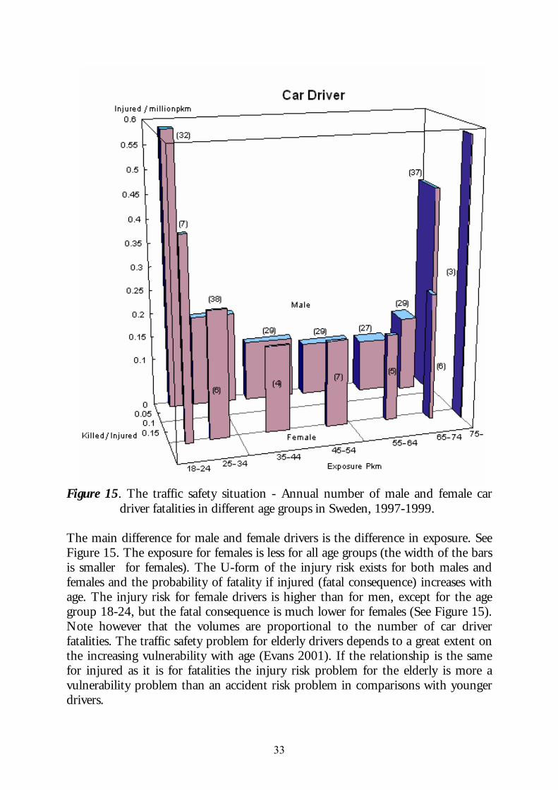
4.5.2 Exposure, risk and consequence in Sweden First, the traffic safety situation is investigated for car drivers (Table 9 and Figure 15). Table 9. Exposure, risk and consequence for car drivers by age and gender.

Car driver – Male Age 1997-1999 18-24 25-34 35-44 45-54 55-64 65-74 75- Million person kilometres per year

2307 7940 8820 8855 5633 2921 890

All injured/Million person kilometres

0.584 0.192 0.126 0.112 0.110 0.159 0.449

Fatalities/All injured 0.024 0.025 0.026 0.030 0.044 0.062 0.093 Car driver – Female Age 1997-1999 18-24 25-34 35-44 45-54 55-64 65-74 75- Million person kilometres per year

1354 3461 4237 3755 2053 713 131

All injured/Million person kilometres

0.417 0.264 0.179 0.179 0.181 0.264 0.582

Fatalities/All injured 0.013 0.007 0.005 0.010 0.013 0.032 0.044

33

Figure 15. The traffic safety situation - Annual number of male and female car

driver fatalities in different age groups in Sweden, 1997-1999. The main difference for male and female drivers is the difference in exposure. See Figure 15. The exposure for females is less for all age groups (the width of the bars is smaller for females). The U-form of the injury risk exists for both males and females and the probability of fatality if injured (fatal consequence) increases with age. The injury risk for female drivers is higher than for men, except for the age group 18-24, but the fatal consequence is much lower for females (See Figure 15). Note however that the volumes are proportional to the number of car driver fatalities. The traffic safety problem for elderly drivers depends to a great extent on the increasing vulnerability with age (Evans 2001). If the relationship is the same for injured as it is for fatalities the injury risk problem for the elderly is more a vulnerability problem than an accident risk problem in comparisons with younger drivers.

34

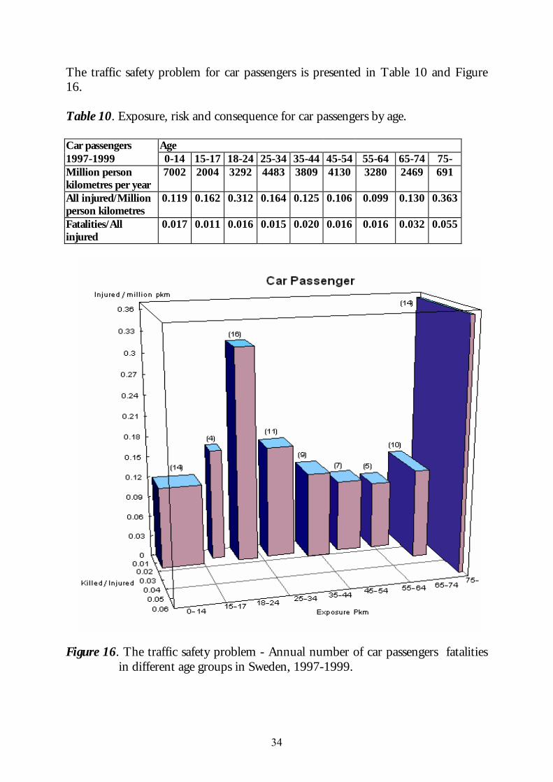
The traffic safety problem for car passengers is presented in Table 10 and Figure 16. Table 10. Exposure, risk and consequence for car passengers by age. Car passengers Age 1997-1999 0-14 15-17 18-24 25-34 35-44 45-54 55-64 65-74 75- Million person kilometres per year

7002 2004 3292 4483 3809 4130 3280 2469 691

All injured/Million person kilometres

0.119 0.162 0.312 0.164 0.125 0.106 0.099 0.130 0.363

Fatalities/All injured

0.017 0.011 0.016 0.015 0.020 0.016 0.016 0.032 0.055

Figure 16. The traffic safety problem - Annual number of car passengers fatalities

in different age groups in Sweden, 1997-1999.

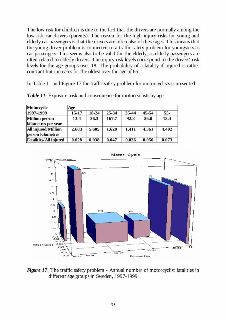
35

The low risk for children is due to the fact that the drivers are normally among the low risk car drivers (parents). The reason for the high injury risks for young and elderly car passengers is that the drivers are often also of these ages. This means that the young driver problem is connected to a traffic safety problem for youngsters as car passengers. This seems also to be valid for the elderly, as elderly passengers are often related to elderly drivers. The injury risk levels correspond to the drivers' risk levels for the age groups over 18. The probability of a fatality if injured is rather constant but increases for the oldest over the age of 65. In Table 11 and Figure 17 the traffic safety problem for motorcyclists is presented. Table 11. Exposure, risk and consequence for motorcyclists by age. Motorcycle Age 1997-1999 15-17 18-24 25-34 35-44 45-54 55- Million person kilometres per year

13.4 36.3 167.7 92.8 26.0 13.4

All injured/Million person kilometres

2.683 5.605 1.620 1.411 4.361 4.402

Fatalities/All injured 0.028 0.038 0.047 0.036 0.056 0.073

Figure 17. The traffic safety problem - Annual number of motorcyclist fatalities in

different age groups in Sweden, 1997-1999

36

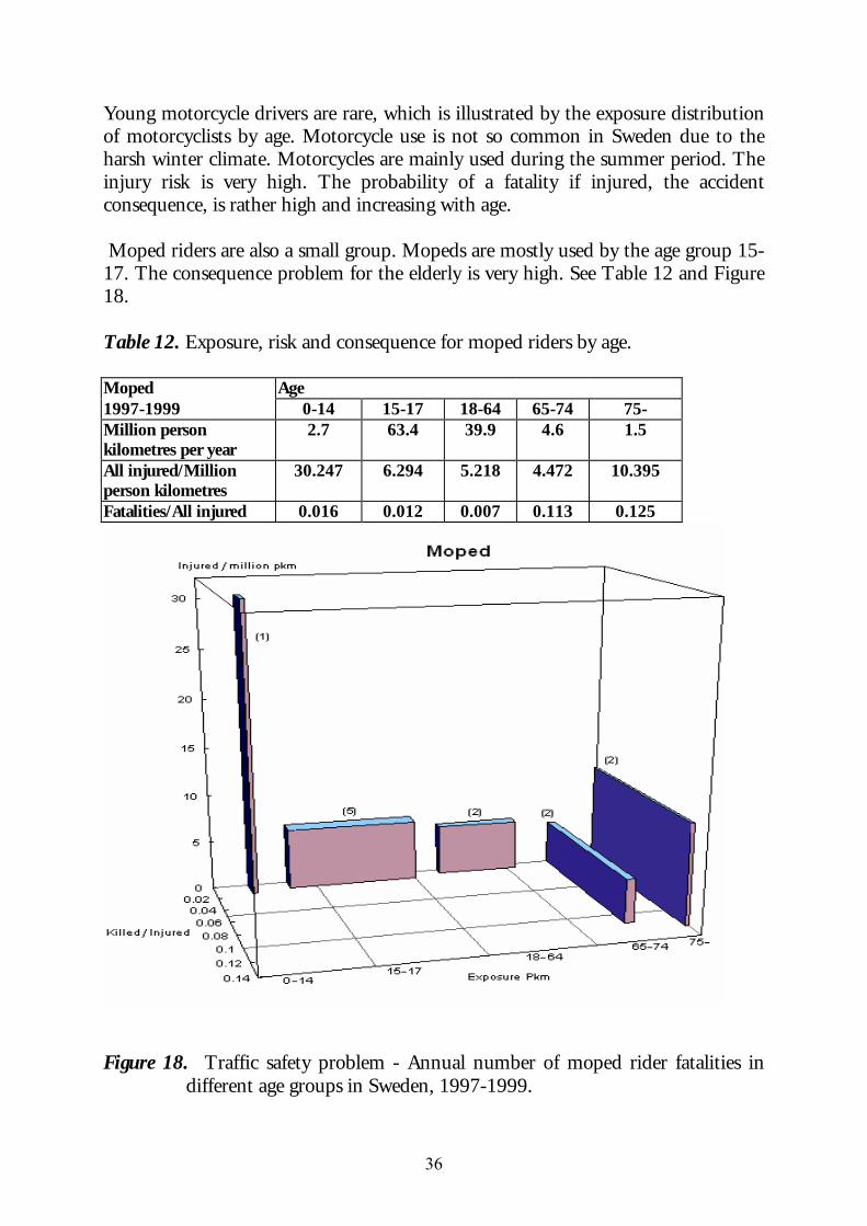
Young motorcycle drivers are rare, which is illustrated by the exposure distribution of motorcyclists by age. Motorcycle use is not so common in Sweden due to the harsh winter climate. Motorcycles are mainly used during the summer period. The injury risk is very high. The probability of a fatality if injured, the accident consequence, is rather high and increasing with age. Moped riders are also a small group. Mopeds are mostly used by the age group 15-17. The consequence problem for the elderly is very high. See Table 12 and Figure 18.

Table 12. Exposure, risk and consequence for moped riders by age.

Moped Age 1997-1999 0-14 15-17 18-64 65-74 75- Million person kilometres per year

2.7 63.4 39.9 4.6 1.5

All injured/Million person kilometres

30.247 6.294 5.218 4.472 10.395

Fatalities/All injured 0.016 0.012 0.007 0.113 0.125

Figure 18. Traffic safety problem - Annual number of moped rider fatalities in

different age groups in Sweden, 1997-1999.

37

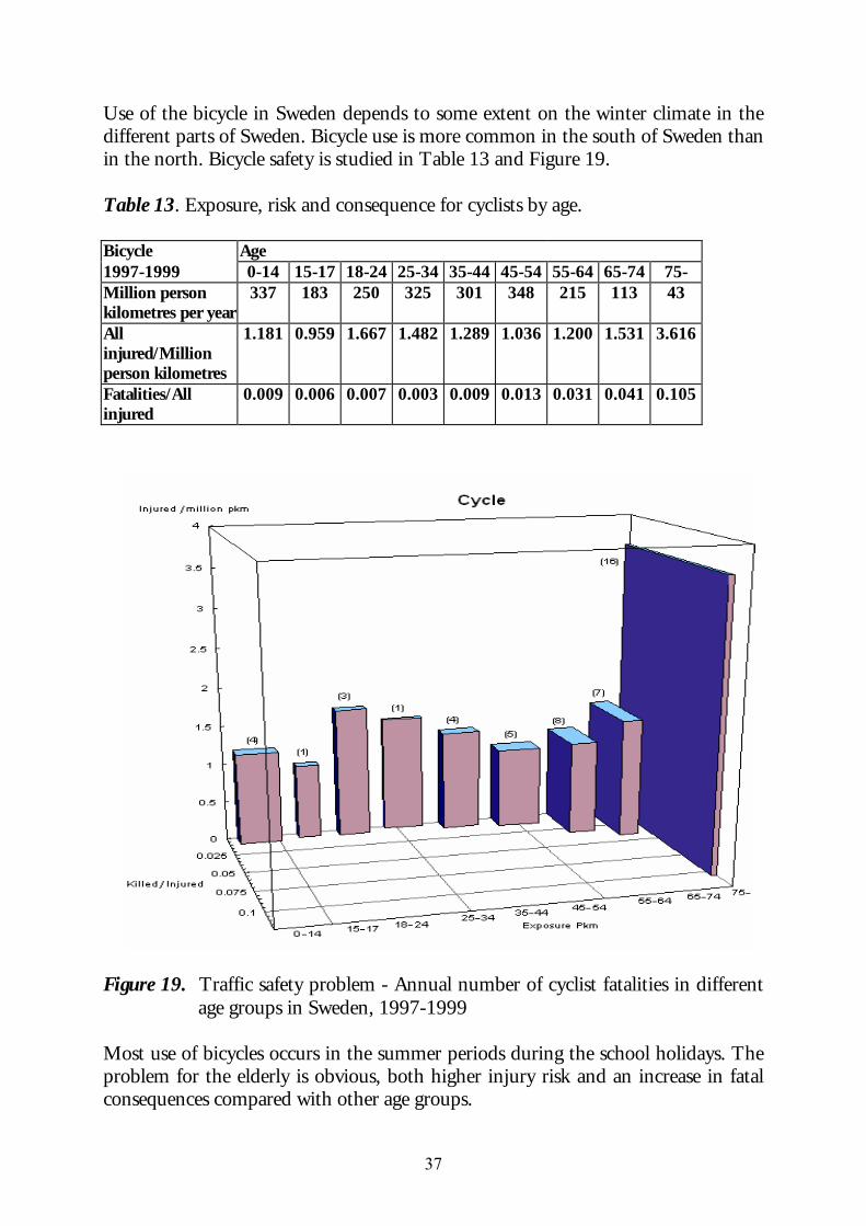
Use of the bicycle in Sweden depends to some extent on the winter climate in the different parts of Sweden. Bicycle use is more common in the south of Sweden than in the north. Bicycle safety is studied in Table 13 and Figure 19. Table 13. Exposure, risk and consequence for cyclists by age.

Bicycle Age 1997-1999 0-14 15-17 18-24 25-34 35-44 45-54 55-64 65-74 75- Million person kilometres per year

337 183 250 325 301 348 215 113 43

All injured/Million person kilometres

1.181 0.959 1.667 1.482 1.289 1.036 1.200 1.531 3.616

Fatalities/All injured

0.009 0.006 0.007 0.003 0.009 0.013 0.031 0.041 0.105

Figure 19. Traffic safety problem - Annual number of cyclist fatalities in different

age groups in Sweden, 1997-1999 Most use of bicycles occurs in the summer periods during the school holidays. The problem for the elderly is obvious, both higher injury risk and an increase in fatal consequences compared with other age groups.

38

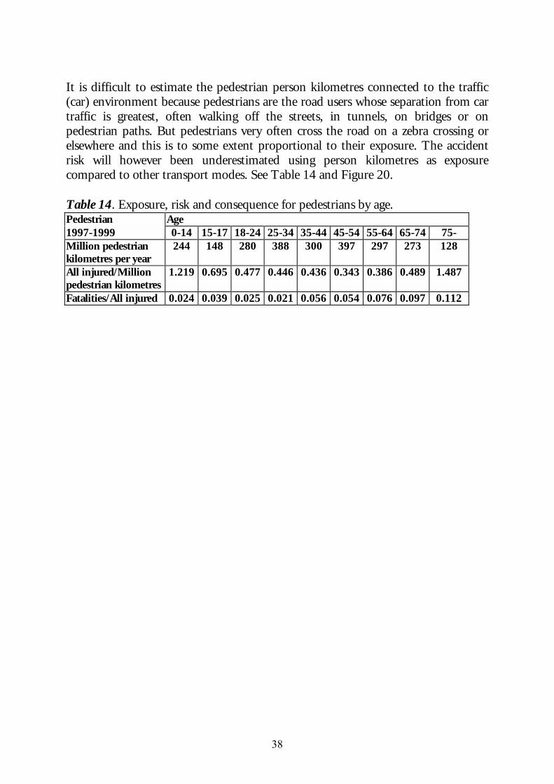
It is difficult to estimate the pedestrian person kilometres connected to the traffic (car) environment because pedestrians are the road users whose separation from car traffic is greatest, often walking off the streets, in tunnels, on bridges or on pedestrian paths. But pedestrians very often cross the road on a zebra crossing or elsewhere and this is to some extent proportional to their exposure. The accident risk will however been underestimated using person kilometres as exposure compared to other transport modes. See Table 14 and Figure 20. Table 14. Exposure, risk and consequence for pedestrians by age. Pedestrian Age 1997-1999 0-14 15-17 18-24 25-34 35-44 45-54 55-64 65-74 75- Million pedestrian kilometres per year

244 148 280 388 300 397 297 273 128

All injured/Million pedestrian kilometres

1.219 0.695 0.477 0.446 0.436 0.343 0.386 0.489 1.487

Fatalities/All injured 0.024 0.039 0.025 0.021 0.056 0.054 0.076 0.097 0.112

39

Figure 20. The traffic safety problem-Annual number of pedestrian fatalities in different age groups in Sweden, 1997-1999

40

To be a pedestrian is a great injury problem for the elderly but also for the youngest. The probability of being killed if injured as a pedestrian starts to increase earlier than for other transport modes. The consequence is rather high from age 35 and increases with age. The three-dimensional presentations concerning injury risk, number of injured per million person kilometres, show a strong U-shape for age groups of drivers of different transportation modes and pedestrians. Cyclists are an exception where the accident risk increases more or less with age. The injury risk for car passengers in different age groups has a close relation to the risk of drivers in different age groups. The risk of children is connected to parents as drivers with a rather low risk, and younger and elderly passengers have in most cases drivers of the same age with high injury risk as a result. The fatal consequence, number of fatalities of all injured, generally increases with age, which means that the injury risk and the fatal consequence together create an increasing fatality risk with age (the side areas in the figures). The elderly have high fatality risks as car passengers, pedestrians and cyclists. Exposure, million person kilometres, as motor vehicle drivers increases with age and reaches a maximum and starts to decrease when the drivers become old (an opposite U-form). This last is valid for all the elderly in the transport system. This means that the accident risk and the size of exposure, at least for age groups of drivers, have a negative correlation. Both the accident risk and the accident consequence increase with age for the elderly. The age of the elderly has a negative correlation with exposure, the older having less exposure. The above figures are a set of examples to illustrate the traffic safety problems (the size of the boxes). The configuration of the box confirms, simultaneously, whether it is an exposure problem, an injury risk problem or a high risk of being killed if injured, a consequence problem. The method tries to include as many relevant and possible indicators/dimensions at the same time as possible. As the objective is to reduce the safety problems, either the risk, consequence or exposure can be reduced. In the process it is also important that the most acceptable, most effective or cost-effective measures are used.

Just looking at accidents, casualty or fatality figures alone will normally give very little information of the ways in which exposure and different terms of risks or consequences have changed and what kind of measures are most important in order to improve the safety situation.

41

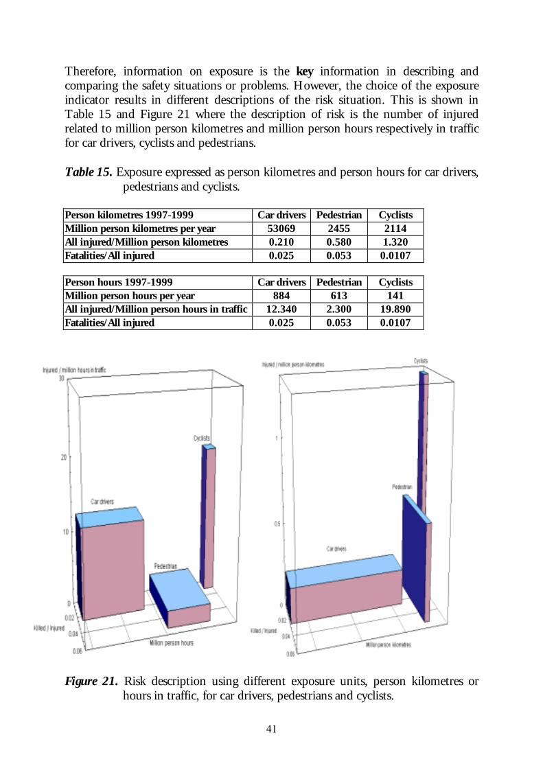
Therefore, information on exposure is the key information in describing and comparing the safety situations or problems. However, the choice of the exposure indicator results in different descriptions of the risk situation. This is shown in Table 15 and Figure 21 where the description of risk is the number of injured related to million person kilometres and million person hours respectively in traffic for car drivers, cyclists and pedestrians. Table 15. Exposure expressed as person kilometres and person hours for car drivers,

pedestrians and cyclists. Person kilometres 1997-1999 Car drivers Pedestrian Cyclists Million person kilometres per year 53069 2455 2114 All injured/Million person kilometres 0.210 0.580 1.320 Fatalities/All injured 0.025 0.053 0.0107 Person hours 1997-1999 Car drivers Pedestrian Cyclists Million person hours per year 884 613 141 All injured/Million person hours in traffic 12.340 2.300 19.890 Fatalities/All injured 0.025 0.053 0.0107

Figure 21. Risk description using different exposure units, person kilometres or hours in traffic, for car drivers, pedestrians and cyclists.

42

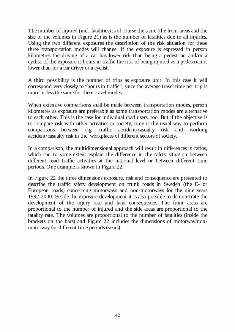
The number of injured (incl. fatalities) is of course the same (the front areas and the size of the volumes in Figure 21) as is the number of fatalities due to all injuries. Using the two different exposures the description of the risk situation for these three transportation modes will change. If the exposure is expressed in person kilometres the driving of a car has lower risk than being a pedestrian and/or a cyclist. If the exposure is hours in traffic the risk of being injured as a pedestrian is lower than for a car driver or a cyclist. A third possibility is the number of trips as exposure unit. In this case it will correspond very closely to “hours in traffic”, since the average travel time per trip is more or less the same for these travel modes. When extensive comparisons shall be made between transportation modes, person kilometres as exposure are preferable as some transportation modes are alternative to each other. This is the case for individual road users, too. But if the objective is to compare risk with other activities in society, time is the usual way to perform comparisons between e.g. traffic accident/casualty risk and working accident/casualty risk in the workplaces of different sectors of society. In a comparison, the multidimensional approach will result in differences in ratios, which can to some extent explain the difference in the safety situation between different road traffic activities at the national level or between different time periods. One example is shown in Figure 22. In Figure 22 the three dimensions exposure, risk and consequence are presented to describe the traffic safety development on trunk roads in Sweden (the E- or European roads) concerning motorways and non-motorways for the nine years 1992-2000. Beside the exposure development it is also possible to demonstrate the development of the injury rate and fatal consequence. The front areas are proportional to the number of injured and the side areas are proportional to the fatality rate. The volumes are proportional to the number of fatalities (inside the brackets on the bars) and Figure 22 includes the dimensions of motorway/non-motorway for different time periods (years).

43

Figure 22. The three-dimensional illustration, exposure, risk and consequence, for

the non-motorways and motorways of the trunk roads in Sweden 1992-2000

Figure 22 shows no effect of road improvements on the non-motorway European roads in Sweden during the 90s. Even if the exposure is increasing on motorways (the width of the front bars) and decreasing on non-motorways (the width of the back bars) the injury risk increases a little (the height of the bars) and the fatal consequence decreases much (the depth of the bars) on motorways and to some extent on non-motorways on European roads in Sweden during the 1992-2000. Both the injury rate and the fatal consequences are much lower on motorways than on non-motorways (about half). The positive safety development in the period 1992-2000 on European roads in Sweden is achieved by lower fatal consequence and not by lower injury accident rate, which is illustrated in Figure 22. The unchanged risk values should not be interpreted so that they could be used for e.g. prediction of numbers of accidents

Million vehicle kilometres

44

or casualties if exposure is changed. The linearity between accidents or casualties has been treated by e.g. Ezra Hauer (Hauer, E. 2000).

45

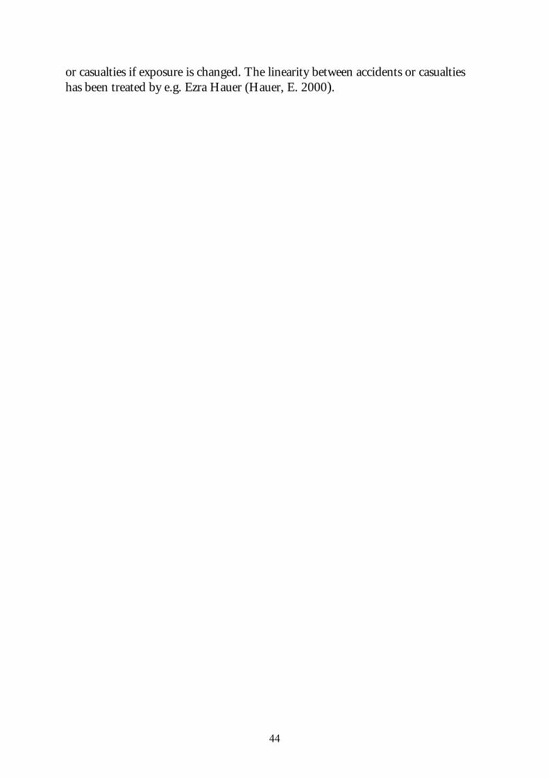
4.6 Ratio chain expansion The theory of the three dimensions, exposure, risk and consequence, can be expanded to a chain of ratios/dimensions where the numerator in the last ratio corresponds to the described safety situation. This tautology have also been presented by Asmussen & Kranenburg, 1982. In principle, the numerator shall be the same as the denominator in the next ratio. This means that the three concepts can be described by several ratios without changing the magnitude of the original safety situation. The number of fatalities related to the number of inhabitants can be expressed as a chain of products consisting of the estimate of the average exposure per inhabitant, the accident rate and the average number of fatalities in an accident.

=

AccidentsFatalities*

ExposureAccidents*

sInhabitantExposure

sInhabitantfatalities ofNumber (4.7)

The exposure term can range from e.g. inhabitants, licence holders, vehicles, vehicle kilometres to person kilometres.

kilometres Vehiclekilometres Person *

Vehicleskilometres Vehicle*

LicencesVehicles*

sInhabitantLicences*sInhabitant (4.8)

In the same way the risk and consequence term can consist of several ratios

=

accidentsInjury accidents Fatal*

AccidentsaccidentsInjury *

ExposureAccidents

Exposureaccidents Fatal (4.9)

or

=

injured and Fatalities

Fatalities*Accidents

injured and Fatalities*ExposureAccidents

ExposureFatalities (4.10)

The first expression (4.9) is accident orientated and if the ratio

accidents FatalFatalities *(-------------------) is added it corresponds to the second

expression (4.10) which is injury related. The consequence term can, for example, be treated as

=

injuredseverely and FatalitiesFatalities*

injured and Fatalitiesinjuredseverely and Fatalities*

Accidentsinjured and Fatalities

AccidentsFatalities (4.11)

46

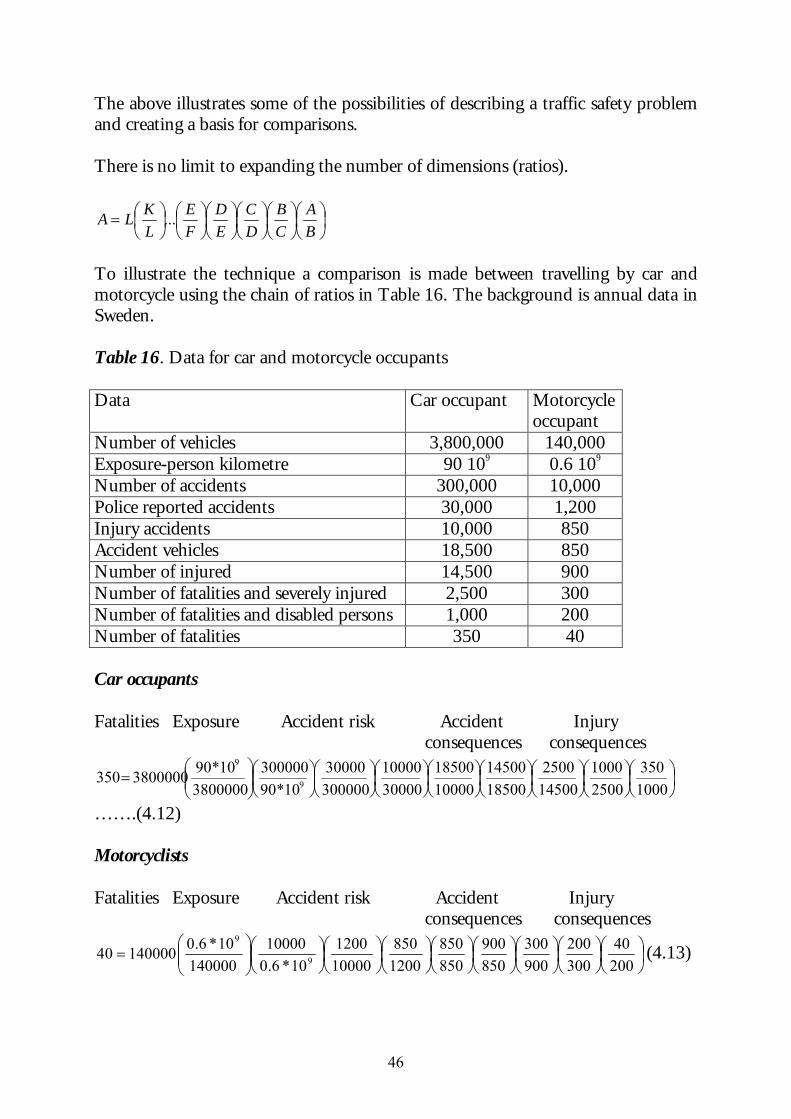
The above illustrates some of the possibilities of describing a traffic safety problem and creating a basis for comparisons. There is no limit to expanding the number of dimensions (ratios).

=

BA

CB

DC

ED

FE

LKLA ...

To illustrate the technique a comparison is made between travelling by car and motorcycle using the chain of ratios in Table 16. The background is annual data in Sweden. Table 16. Data for car and motorcycle occupants

Data Car occupant Motorcycle

occupant Number of vehicles 3,800,000 140,000 Exposure-person kilometre 90 109 0.6 109

Number of accidents 300,000 10,000 Police reported accidents 30,000 1,200 Injury accidents 10,000 850 Accident vehicles 18,500 850 Number of injured 14,500 900 Number of fatalities and severely injured 2,500 300 Number of fatalities and disabled persons 1,000 200 Number of fatalities 350 40 Car occupants Fatalities Exposure Accident risk Accident Injury consequences consequences

=

1000350

25001000

145002500

1850014500

1000018500

3000010000

30000030000

10*90300000

380000010*903800000350 9

9

…….(4.12) Motorcyclists Fatalities Exposure Accident risk Accident Injury consequences consequences

=

20040

300200

900300

850900

850850

1200850

100001200

10*.6010000

14000010*.6014000004 9

9

(4.13)

47

Table 17. Chain of ratios for car and motorcycle occupant Ratio Car occupant Motorcyclist Occupant distance/vehicle 23684 km 4286 km Accident risk = Number of accidents per million person kilometres

3.3 16.7

Proportion of accidents reported by the police 0.10 0.12 Proportion of injury accidents of police reported accidents

0.33 0.71

Involved vehicles per injury accident 1.85 1.00 Injured/injury accident vehicle 0.78 1.06 Number of fatalities and severely injured/injured

0.17 0.33

Number of fatalities and disabled persons/ Number of fatalities and severely injured

0.40 0.67

Number of fatalities /number of fatalities and disabled persons

0.35 0.20

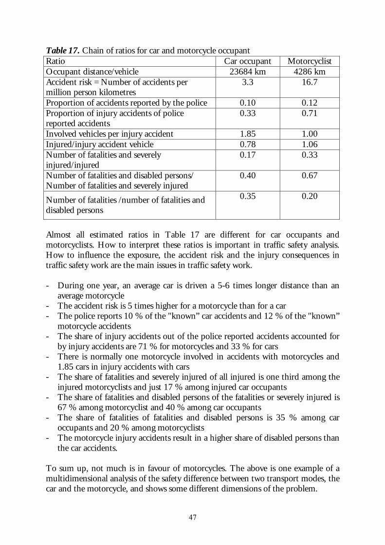
Almost all estimated ratios in Table 17 are different for car occupants and motorcyclists. How to interpret these ratios is important in traffic safety analysis. How to influence the exposure, the accident risk and the injury consequences in traffic safety work are the main issues in traffic safety work. - During one year, an average car is driven a 5-6 times longer distance than an

average motorcycle - The accident risk is 5 times higher for a motorcycle than for a car - The police reports 10 % of the "known” car accidents and 12 % of the "known”

motorcycle accidents - The share of injury accidents out of the police reported accidents accounted for

by injury accidents are 71 % for motorcycles and 33 % for cars - There is normally one motorcycle involved in accidents with motorcycles and

1.85 cars in injury accidents with cars - The share of fatalities and severely injured of all injured is one third among the

injured motorcyclists and just 17 % among injured car occupants - The share of fatalities and disabled persons of the fatalities or severely injured is

67 % among motorcyclist and 40 % among car occupants - The share of fatalities of fatalities and disabled persons is 35 % among car

occupants and 20 % among motorcyclists - The motorcycle injury accidents result in a higher share of disabled persons than

the car accidents. To sum up, not much is in favour of motorcycles. The above is one example of a multidimensional analysis of the safety difference between two transport modes, the car and the motorcycle, and shows some different dimensions of the problem.

48

4.7 Conclusions The traffic safety problem is normally a multidimensional problem. In order to realise the structure of the multidimensional problem it can be of some value to try to visualize different dimensions of different traffic safety problems. It is natural to start with the dimensions exposure, risk and consequence. By choosing the right risk and consequence indicators the illustration shows simultaneously some other dimensions. This last technique can be used to expand the chain of ratios, which all represent other dimensions of the traffic safety problem. This will not solve the traffic safety problem but will in some way prevent the “disappearance" of the original traffic safety problem in the traffic safety analysis work. The three-dimensional figures seems to assist road safety experts in the analysis of the safety problem in addition to conventional tables and may also influence the identification of the most important problems to some extent. The technique of chain of ratios will not be able to visualize if it corresponds to more than three dimensions. It is however possible to make comparisons of several dimensions of the traffic safety situation between traffic populations as shown between car and motorcycle occupants.

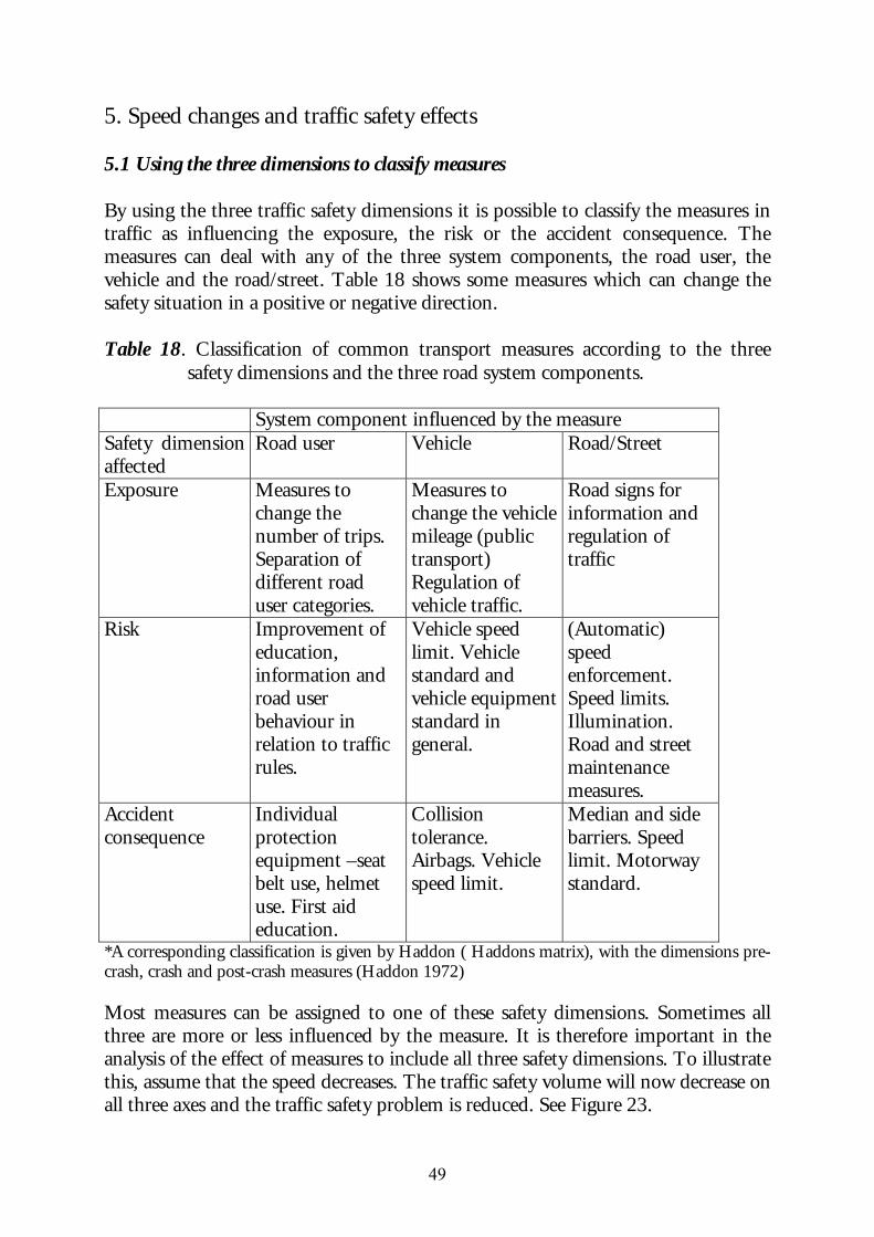
49

5. Speed changes and traffic safety effects 5.1 Using the three dimensions to classify measures By using the three traffic safety dimensions it is possible to classify the measures in traffic as influencing the exposure, the risk or the accident consequence. The measures can deal with any of the three system components, the road user, the vehicle and the road/street. Table 18 shows some measures which can change the safety situation in a positive or negative direction. Table 18. Classification of common transport measures according to the three

safety dimensions and the three road system components. System component influenced by the measure Safety dimension affected

Road user Vehicle Road/Street

Exposure Measures to change the number of trips. Separation of different road user categories.

Measures to change the vehicle mileage (public transport) Regulation of vehicle traffic.

Road signs for information and regulation of traffic

Risk Improvement of education, information and road user behaviour in relation to traffic rules.

Vehicle speed limit. Vehicle standard and vehicle equipment standard in general.

(Automatic) speed enforcement. Speed limits. Illumination. Road and street maintenance measures.

Accident consequence

Individual protection equipment –seat belt use, helmet use. First aid education.

Collision tolerance. Airbags. Vehicle speed limit.

Median and side barriers. Speed limit. Motorway standard.

*A corresponding classification is given by Haddon ( Haddons matrix), with the dimensions pre-crash, crash and post-crash measures (Haddon 1972) Most measures can be assigned to one of these safety dimensions. Sometimes all three are more or less influenced by the measure. It is therefore important in the analysis of the effect of measures to include all three safety dimensions. To illustrate this, assume that the speed decreases. The traffic safety volume will now decrease on all three axes and the traffic safety problem is reduced. See Figure 23.

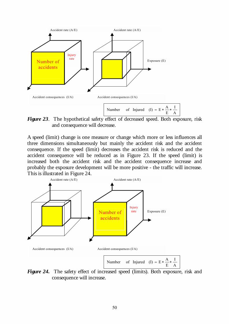
50

Number ofaccidents

Injuryrate

Accident rate (A/E) Accident rate (A/E)

Accident consequences (I/A) Accident consequences (I/A)

Exposure (E)

AI

EAE(I) Injured ofNumber ∗∗=

Figure 23. The hypothetical safety effect of decreased speed. Both exposure, risk

and consequence will decrease. A speed (limit) change is one measure or change which more or less influences all three dimensions simultaneously but mainly the accident risk and the accident consequence. If the speed (limit) decreases the accident risk is reduced and the accident consequence will be reduced as in Figure 23. If the speed (limit) is increased both the accident risk and the accident consequence increase and probably the exposure development will be more positive - the traffic will increase. This is illustrated in Figure 24.

Number ofaccidents

Injuryrate

Accident rate (A/E) Accident rate (A/E)

Accident consequences (I/A) Accident consequences (I/A)

Exposure (E)

AI

EAE(I) Injured ofNumber ∗∗=

Figure 24. The safety effect of increased speed (limits). Both exposure, risk and

consequence will increase.

51

A speed increase in the road system can therefore eliminate the effect of other measures taken to improve the safety situation. From this point of view, speed is of very great interest and important for the traffic safety situation and the traffic safety work. An attempt to estimate the change in safety if the speed is changed is presented in the next section. The model concerns both the accident risk and the accident consequence. 5.2 Speed and accidents The aim of traffic safety work is to avoid injuries in traffic accidents, especially serious injuries and fatalities. The first way is of course to avoid the injury accident and the second way is to reduce the consequences to persons involved in the accident when it occurs. It is very difficult to avoid all traffic injury accidents and meanwhile we have to reduce their severe consequences. Three main traffic accident types can be identified. The first one is collision between motor vehicles. To avoid serious injury accidents the collision speed must be low or collision angles small. This is to some extent realised in urban areas. In rural areas, however, head-on collisions between motor vehicles often result in fatalities due to the high speed and/or a high vehicle mass. Another accident type is collision between a motor vehicle and a pedestrian or cyclist. The severity of the injuries of the injured pedestrian/cyclist depends on the speed and the mass of the motor vehicle. A lot of efforts are made to separate pedestrians/cyclists from motor vehicles when the speeds of the motor vehicles are high. In some urban areas the speeds of motor vehicles are made very low in order to avoid severe injuries to pedestrians/cyclists and thus allow some mixed traffic. The third accident type is motor vehicle collision with a fixed obstacle at the roadside and is most common. Fatalities are frequent if the motor vehicle at high speed hits large fixed obstacles such as poles, trees etc. It is therefore obvious that a reduction in the speed level leads to a safety improvement for all types of traffic accidents. This is also confirmed by many investigations around the world, where an analysis of the safety situation and the speed level has been made before and after a change in speed limits in different environments. (Nilsson 1977, 1981a, 1984b, 1990 and Elvik et al 1997)). A speed change results in many direct effects related to the drivers or the road users, which are important for the safety situation.

52

- The braking distance of motor vehicles is changed - The change in speed together with the possible change in reaction time changes

the distance driven before action - The collision speed is changed - The probability for pedestrians/cyclists to avoid an accident with a motor

vehicle is changed - The force/violence to human organs in an accident is changed If the speed is decreased the braking distance decreases according to the second power of the speed. If the braking distance is 100 metres on a specific road surface at the speed of 100 km/h it is just 81 metres at the speed of 90 km/h. If braking is needed to avoid a collision, the distance driven before braking due to the reaction time is proportional to the speed. If the reaction time is one (1) second this distance is 25 metres at the speed of 90 km/h and 28 metres at the speed of 100 km/h. The distance to stop a car is thus the distance driven before braking and the braking distance. (Evans 1991) In reality there is a variation in speeds in traffic, a variation in braking distances, a variation in different vehicles and road users etc.. In order to have a simple model, all this can be aggregated in a model which is based on a relationship between accidents or injured and the average speed changes of the motor traffic. The collision speeds of the colliding vehicles give rise to a kinetic energy which is absorbed by the vehicle constructions, passive safety measures and the involved car occupants. Even if a lot of measures are taken to try to protect the car occupants from being injured, the forces caused by the deceleration due to the sudden transformation of kinetic energy may lead to injuries in the form of fractures or injuries to important body organs. Head injuries (brain and neck) together with leg injuries are the most common injuries which need hospital treatment (Krafft 1997). The head and the legs are the most vulnerable parts of the body. When cars collide with pedestrians, cyclists or animals, almost all forces are concentrated on the vulnerable road user or the animal. These accidents are very serious to the vulnerable participant and will in collision with big and heavy animals (elks) sometimes also result in a car occupant injury. There are some investigations of the collision speed and the probability of pedestrian fatality in collisions between cars and pedestrians. The relationship between increased collision speed and the increased probability of a pedestrian fatality coincides with the increase in kinetic energy (Pasanen 1992, Spolander 1999).

53

When a car hits hard fixed obstacles in the roadside the car occupants may be injured. The harder the obstacle, the higher are the forces on the body due to the deceleration (Ljungblad 2000). The higher the speed in an accident, the greater is the probability that someone will be injured. The higher the speed in an injury accident, the greater is the probability that someone is killed and the accident becomes a fatal accident (Ashton et al 1977, Nilsson, G. 1984b). Naturally, the more persons involved in an accident, the greater are the probabilities of injuries or fatalities. Increased speed leads to higher kinetic energies among the vehicles and the kinetic energy is proportional to the square of the speed. It is then natural to assume that the traffic safety situation is governed by the kinetic energy, and if the kinetic energy changes the traffic safety situation changes. There are a lot of statistical accident investigations concerning the effect on safety of changed speed limits (Nilsson 1977, 1981, 1984, and 1990). In most cases these studies are before and after studies sometimes with control roads where the speed limit was unchanged. The estimated effect is a total effect of what has happened concerning the traffic accidents between the before and after periods. The actual safety effect of the change in speed limit on accidents is obtained by taking into account the controls or estimates of the changes in traffic development between the periods (Elvik et al 1997). The experience from these statistical investigations is very similar and shows that the change in injury accidents can be regarded as proportional to the square of the relative change in speed i.e. the change in kinetic energy in the system. The same seems to be valid for the proportion of fatal accidents among injury accidents. Hence, the change in fatal accidents is then proportional to the fourth power of the relative change in speed. All these investigations mainly describe the safety effect of a speed limit change between a before and an after period and present an estimate of the change in speed between the periods. In addition to a possible change in the traffic volume there can be some other changes which probably influence the traffic safety situation. These changes are sometimes mentioned but seldom quantified in terms of traffic safety (Elvik et al 1997). As a lot of other measures are also taken to improve the traffic safety situation, many measures result in a change in speeds, for example improvement of the road surface, increased width of carriageway, canalisation of intersections etc. Often just the accident or injury effect of the measure itself is estimated even if the effect is partly dependent on changed speed behaviour. In these investigations, the accident

54

or injury effect is normally presented with some qualitative or quantitative comments on speed behaviour (Elvik et al 1997). It is of course natural to investigate the change in speed if the speed limit is changed but less natural if the intention was to improve the safety situation without changing the speed limit even if the speed changes. For instance, increasing the width of the road normally results in increased safety but the expected safety effect is reduced to some extent due to increased speed (SNRA 2001). Therefore it is important to have information about the magnitude of the change in speed and not only the change in the number and the severity of accidents. In relation to the above it ought to be important to estimate the effect of speed on safety, regardless of whether or not the measure is taken to change the speed. In statistical investigations of changed speed limits it is normal to isolate the speed effect on safety, if everything else which can influence the safety situation is unchanged or controlled for. Let us consider all vehicles (i) of mass (mi) and speed (vi) in a specific road network during a specific period of time. One can regard traffic as the total kinetic energy

prevailing at a specific point of time in the network i.e. 2

2

1

in

ii

vm∑=

.

∑=

n

iim

1

can be regarded as the traffic exposure. Now, if the number or size of the

vehicles increases the traffic (exposure) will increase. When the exposure increases the number of accidents increases. Therefore it is important to control for changes in exposure. A change in speed will affect both the accident risk and the accident consequences. Assume that the composition of traffic (the vehicles and the road users) remains the same after the change in speed. The more kinetic energy there exists in the transport system, the more energy will be absorbed in accidents resulting in an increased number of accidents and injured as well as more serious accidents or injured. This can be illustrated by the official traffic accident statistics - the higher the speed limit the more fatalities there are per fatal accident and more injured per injury accident. This is shown in Table 19 where the average numbers of killed, severely injured and slightly injured per injury accident involving cars are presented (car involved in an accident with only cars involved and at least one car occupant is injured) (Nilsson 1984 b).

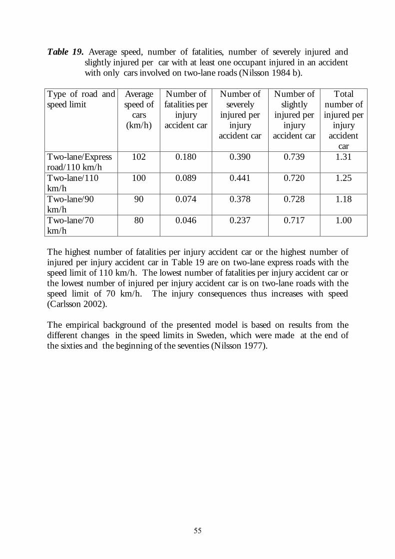
55

Table 19. Average speed, number of fatalities, number of severely injured and slightly injured per car with at least one occupant injured in an accident with only cars involved on two-lane roads (Nilsson 1984 b).

Type of road and speed limit

Average speed of

cars (km/h)

Number of fatalities per

injury accident car

Number of severely

injured per injury

accident car

Number of slightly

injured per injury

accident car

Total number of injured per

injury accident

car Two-lane/Express road/110 km/h

102 0.180 0.390 0.739 1.31

Two-lane/110 km/h

100 0.089 0.441 0.720 1.25

Two-lane/90 km/h

90 0.074 0.378 0.728 1.18

Two-lane/70 km/h

80 0.046 0.237 0.717 1.00

The highest number of fatalities per injury accident car or the highest number of injured per injury accident car in Table 19 are on two-lane express roads with the speed limit of 110 km/h. The lowest number of fatalities per injury accident car or the lowest number of injured per injury accident car is on two-lane roads with the speed limit of 70 km/h. The injury consequences thus increases with speed (Carlsson 2002). The empirical background of the presented model is based on results from the different changes in the speed limits in Sweden, which were made at the end of the sixties and the beginning of the seventies (Nilsson 1977).

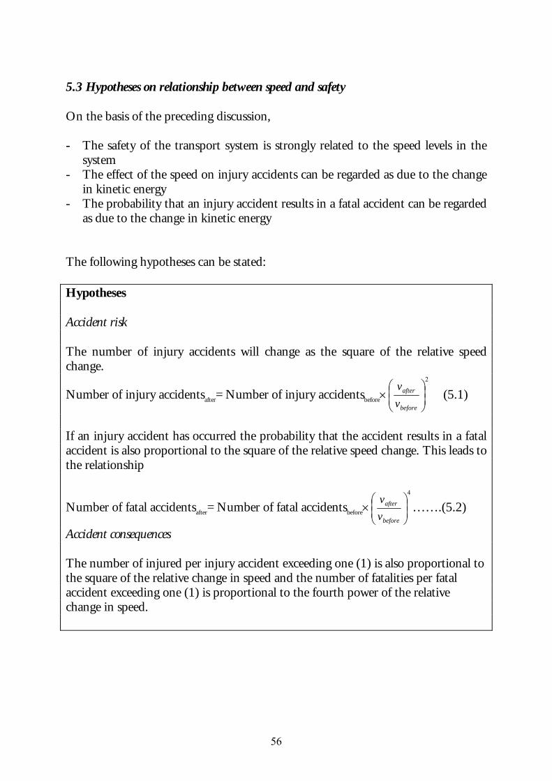
56

5.3 Hypotheses on relationship between speed and safety On the basis of the preceding discussion, - The safety of the transport system is strongly related to the speed levels in the

system - The effect of the speed on injury accidents can be regarded as due to the change

in kinetic energy - The probability that an injury accident results in a fatal accident can be regarded

as due to the change in kinetic energy The following hypotheses can be stated: Hypotheses Accident risk The number of injury accidents will change as the square of the relative speed change.

Number of injury accidentsafter= Number of injury accidentsbefore×2

before

after

vv

(5.1)

If an injury accident has occurred the probability that the accident results in a fatal accident is also proportional to the square of the relative speed change. This leads to the relationship

Number of fatal accidentsafter= Number of fatal accidentsbefore×4

before

after

vv

…….(5.2)

Accident consequences The number of injured per injury accident exceeding one (1) is also proportional to the square of the relative change in speed and the number of fatalities per fatal accident exceeding one (1) is proportional to the fourth power of the relative change in speed.

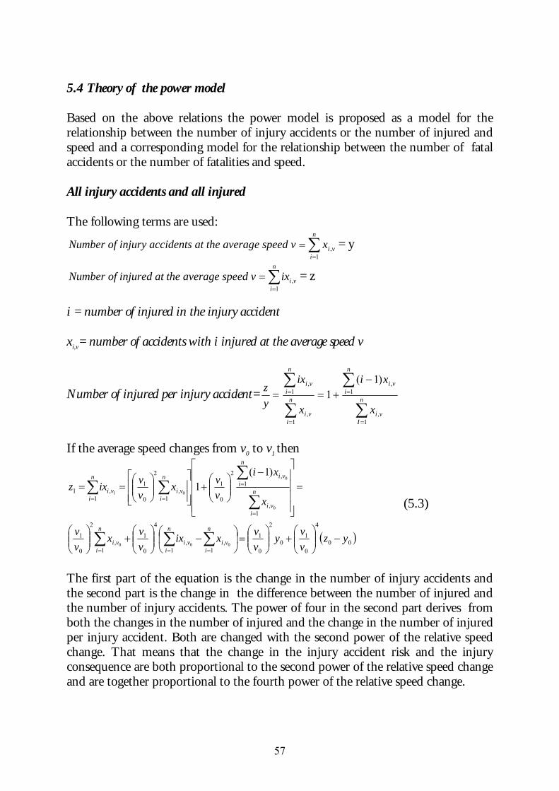
57

5.4 Theory of the power model Based on the above relations the power model is proposed as a model for the relationship between the number of injury accidents or the number of injured and speed and a corresponding model for the relationship between the number of fatal accidents or the number of fatalities and speed. All injury accidents and all injured The following terms are used:

∑=

=n

ivixe speed vthe averagidents at injury accNumber of

1, = y

∑=

=n

iviixge speed v the averainjured atNumber of

1, = z

i = number of injured in the injury accident xi,v= number of accidents with i injured at the average speed v

Number of injured per injury accident= =yz

∑

∑

∑

∑

=

=

=

=

−+= n

Ivi

n

ivi

n

ivi

n

ivi

x

xi

x

ix

1,

1,

1,

1, )1(

1

If the average speed changes from v0 to v1 then

( )00

4

0

10

2

0

1

1 1,,

4

0

1

1,

2

0

1

1,

1,2

0

1

1,

2

0

1

1,1

000

0

0

01

)1(1

yzvvy

vvxix

vvx

vv

x

xi

vvx

vvixz

n

i

n

ivivi

n

ivi

n

ivi

n

ivin

ivi

n

ivi

−

+

=

−

+

=

−

+

==

∑ ∑∑

∑

∑∑∑

= ==

=

=

== (5.3)

The first part of the equation is the change in the number of injury accidents and the second part is the change in the difference between the number of injured and the number of injury accidents. The power of four in the second part derives from both the changes in the number of injured and the change in the number of injured per injury accident. Both are changed with the second power of the relative speed change. That means that the change in the injury accident risk and the injury consequence are both proportional to the second power of the relative speed change and are together proportional to the fourth power of the relative speed change.

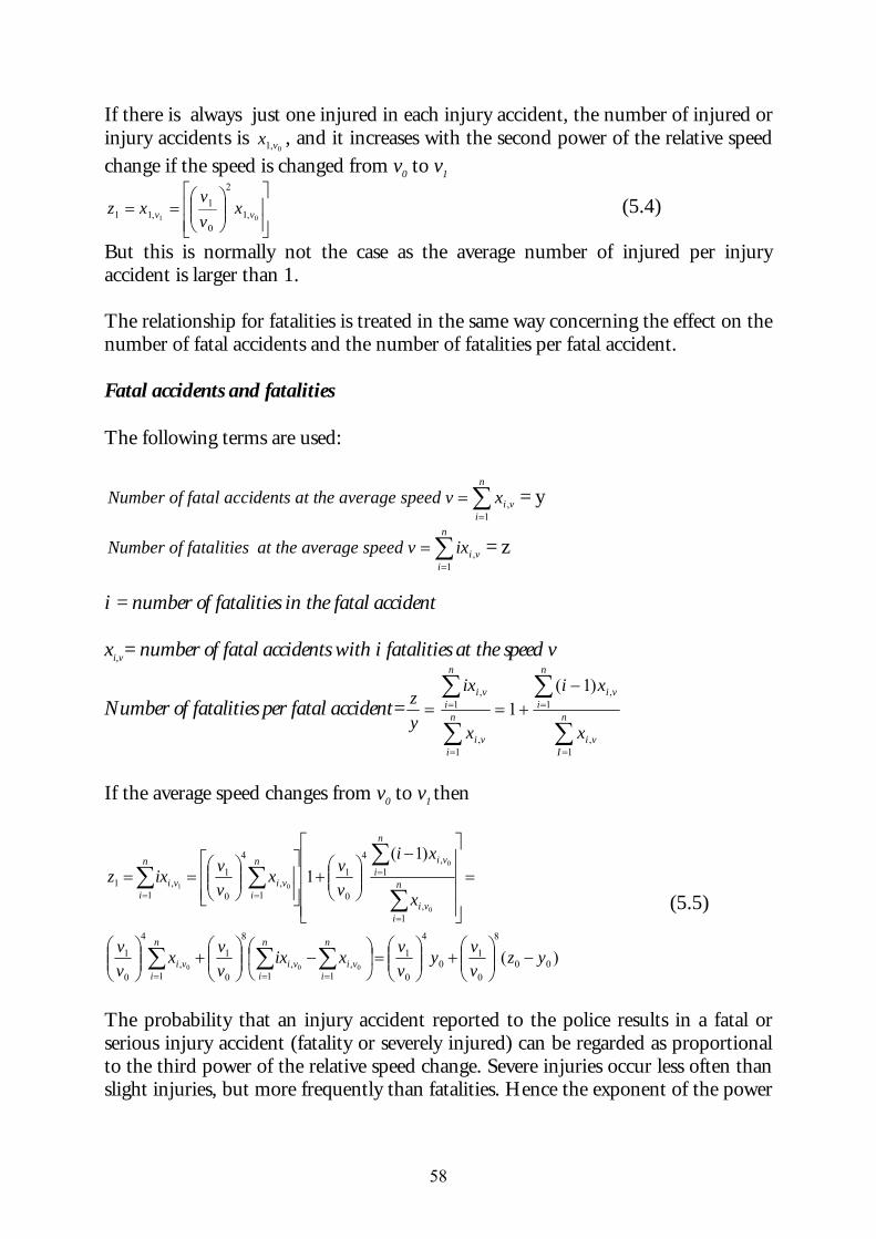
58

If there is always just one injured in each injury accident, the number of injured or injury accidents is

0,1 vx , and it increases with the second power of the relative speed change if the speed is changed from v0 to v1

==

01 ,1

2

0

1,11 vv x

vv

xz (5.4)

But this is normally not the case as the average number of injured per injury accident is larger than 1. The relationship for fatalities is treated in the same way concerning the effect on the number of fatal accidents and the number of fatalities per fatal accident. Fatal accidents and fatalities The following terms are used:

∑=

=n

ivix speed vhe averagedents at tfatal acciNumber of

1, = y

∑=

=n

iviixed vverage spe at the afatalitiesNumber of

1, = z

i = number of fatalities in the fatal accident xi,v= number of fatal accidents with i fatalities at the speed v

Number of fatalities per fatal accident= =yz

∑

∑

∑

∑

=

=

=

=

−+= n

Ivi

n

ivi

n

ivi

n

ivi

x

xi

x

ix

1,

1,

1,

1, )1(

1

If the average speed changes from v0 to v1 then

)(

)1(1

00

8

0

10

4

0

1

1 1,,

8

0

1

1,

4

0

1

1,

1,4

0

1

1,

4

0

1

1,1

000

0

0

01

yzvvy

vvxix

vvx

vv

x

xi

vvx

vvixz

n

i

n

ivivi

n

ivi

n

ivi

n

ivin

ivi

n

ivi

−

+

=

−

+

=

−

+

==

∑ ∑∑

∑

∑∑∑

= ==

=

=

== (5.5)

The probability that an injury accident reported to the police results in a fatal or serious injury accident (fatality or severely injured) can be regarded as proportional to the third power of the relative speed change. Severe injuries occur less often than slight injuries, but more frequently than fatalities. Hence the exponent of the power

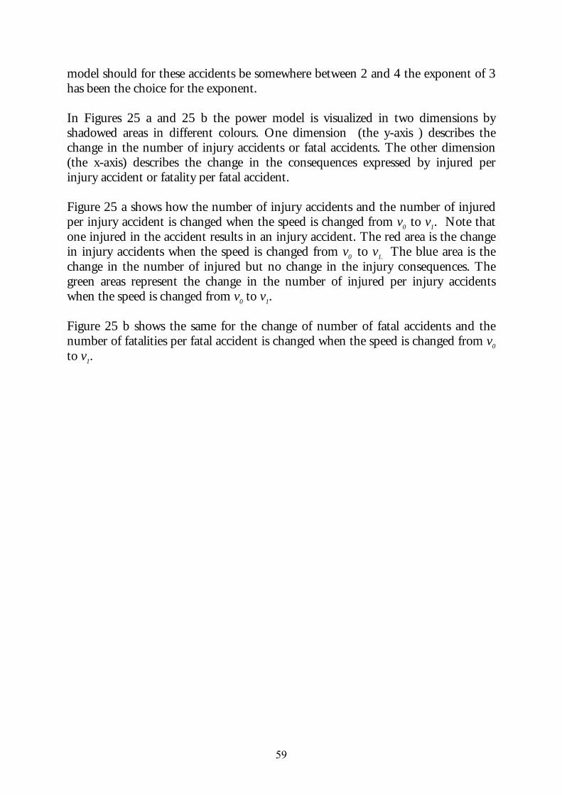
59

model should for these accidents be somewhere between 2 and 4 the exponent of 3 has been the choice for the exponent. In Figures 25 a and 25 b the power model is visualized in two dimensions by shadowed areas in different colours. One dimension (the y-axis ) describes the change in the number of injury accidents or fatal accidents. The other dimension (the x-axis) describes the change in the consequences expressed by injured per injury accident or fatality per fatal accident. Figure 25 a shows how the number of injury accidents and the number of injured per injury accident is changed when the speed is changed from v0 to v1. Note that one injured in the accident results in an injury accident. The red area is the change in injury accidents when the speed is changed from v0 to v1. The blue area is the change in the number of injured but no change in the injury consequences. The green areas represent the change in the number of injured per injury accidents when the speed is changed from v0 to v1. Figure 25 b shows the same for the change of number of fatal accidents and the number of fatalities per fatal accident is changed when the speed is changed from v0

to v1.

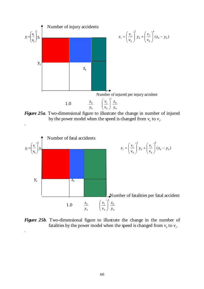
60

Number of injury accidents

0

2

0

11 y

vvy

= )( 00

4

0

10

2

0

11 yz

vvy

vvz −

+

=

y0

z0 Number of injured per injury accident

1.0 0

0

yz

0

0

2

0

1

yz

vv

Figure 25a. Two-dimensional figure to illustrate the change in number of injured by the power model when the speed is changed from v0 to v1.

. Number of fatal accidents

0

4

0

11 y

vvy

= )( 00

8

0

10

4

0

11 yz

vvy

vvz −

+

=

z0 y0 z0

Number of fatalities per fatal accident

1.0 0

0

yz

0

0

4

0

1

yz

vv

Figure 25b. Two-dimensional figure to illustrate the change in the number of

fatalities by the power model when the speed is changed from v0 to v1. .

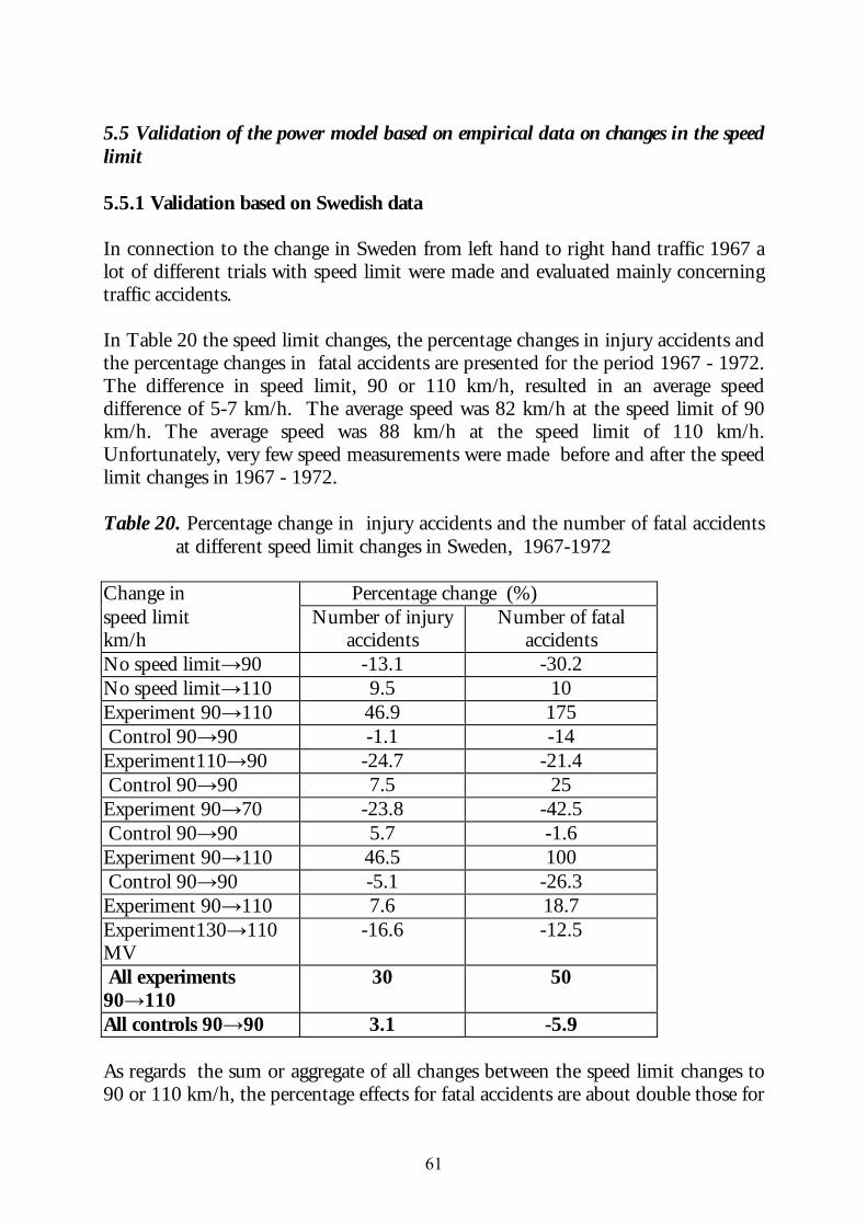
61

5.5 Validation of the power model based on empirical data on changes in the speed limit 5.5.1 Validation based on Swedish data In connection to the change in Sweden from left hand to right hand traffic 1967 a lot of different trials with speed limit were made and evaluated mainly concerning traffic accidents. In Table 20 the speed limit changes, the percentage changes in injury accidents and the percentage changes in fatal accidents are presented for the period 1967 - 1972. The difference in speed limit, 90 or 110 km/h, resulted in an average speed difference of 5-7 km/h. The average speed was 82 km/h at the speed limit of 90 km/h. The average speed was 88 km/h at the speed limit of 110 km/h. Unfortunately, very few speed measurements were made before and after the speed limit changes in 1967 - 1972. Table 20. Percentage change in injury accidents and the number of fatal accidents

at different speed limit changes in Sweden, 1967-1972 Change in Percentage change (%) speed limit km/h

Number of injury accidents

Number of fatal accidents

No speed limit→90 -13.1 -30.2 No speed limit→110 9.5 10 Experiment 90→110 46.9 175 Control 90→90 -1.1 -14 Experiment110→90 -24.7 -21.4 Control 90→90 7.5 25 Experiment 90→70 -23.8 -42.5 Control 90→90 5.7 -1.6 Experiment 90→110 46.5 100 Control 90→90 -5.1 -26.3 Experiment 90→110 7.6 18.7 Experiment130→110 MV

-16.6 -12.5

All experiments 90→110

30 50

All controls 90→90 3.1 -5.9 As regards the sum or aggregate of all changes between the speed limit changes to 90 or 110 km/h, the percentage effects for fatal accidents are about double those for

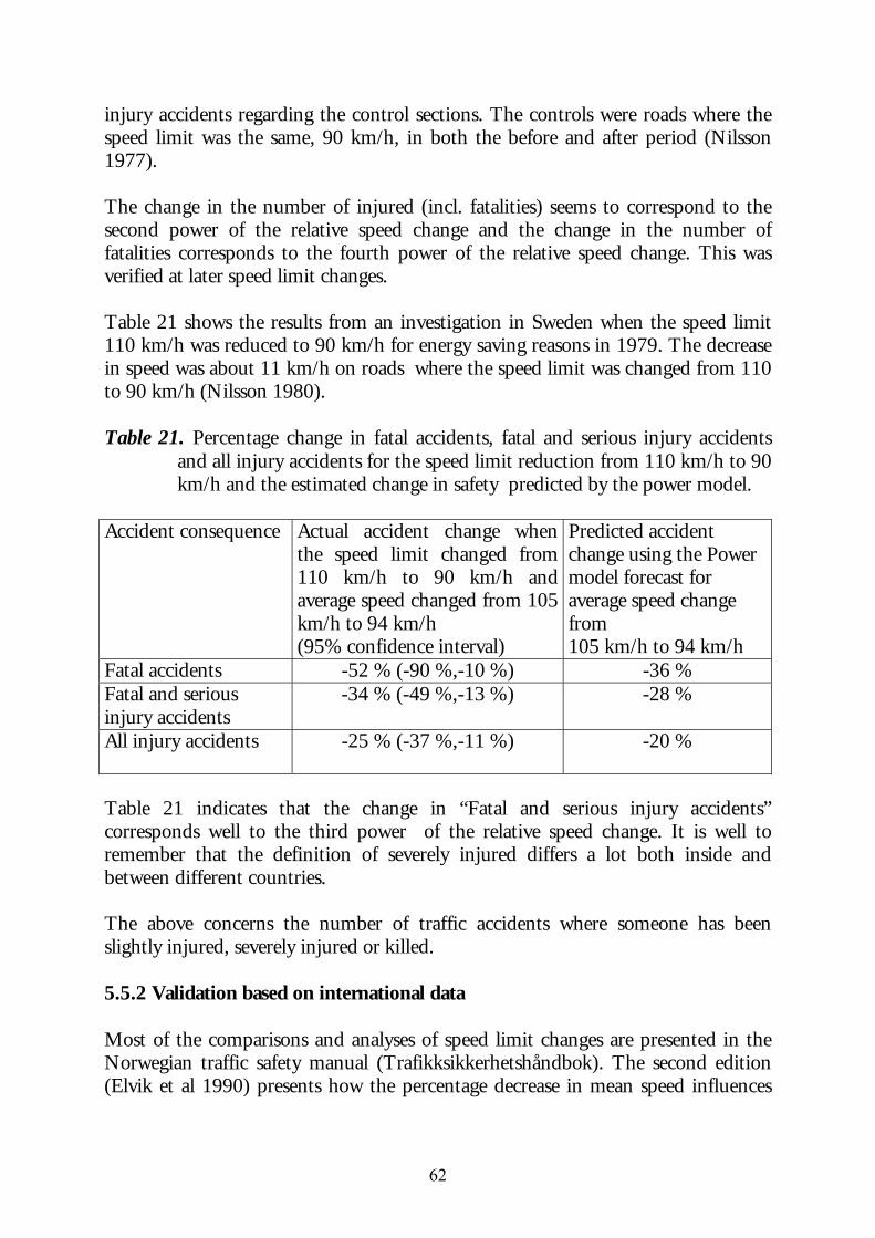
62

injury accidents regarding the control sections. The controls were roads where the speed limit was the same, 90 km/h, in both the before and after period (Nilsson 1977). The change in the number of injured (incl. fatalities) seems to correspond to the second power of the relative speed change and the change in the number of fatalities corresponds to the fourth power of the relative speed change. This was verified at later speed limit changes. Table 21 shows the results from an investigation in Sweden when the speed limit 110 km/h was reduced to 90 km/h for energy saving reasons in 1979. The decrease in speed was about 11 km/h on roads where the speed limit was changed from 110 to 90 km/h (Nilsson 1980). Table 21. Percentage change in fatal accidents, fatal and serious injury accidents

and all injury accidents for the speed limit reduction from 110 km/h to 90 km/h and the estimated change in safety predicted by the power model.

Accident consequence Actual accident change when

the speed limit changed from 110 km/h to 90 km/h and average speed changed from 105 km/h to 94 km/h (95% confidence interval)

Predicted accident change using the Power model forecast for average speed change from 105 km/h to 94 km/h

Fatal accidents -52 % (-90 %,-10 %) -36 % Fatal and serious injury accidents

-34 % (-49 %,-13 %) -28 %

All injury accidents -25 % (-37 %,-11 %) -20 %

Table 21 indicates that the change in “Fatal and serious injury accidents” corresponds well to the third power of the relative speed change. It is well to remember that the definition of severely injured differs a lot both inside and between different countries. The above concerns the number of traffic accidents where someone has been slightly injured, severely injured or killed. 5.5.2 Validation based on international data Most of the comparisons and analyses of speed limit changes are presented in the Norwegian traffic safety manual (Trafikksikkerhetshåndbok). The second edition (Elvik et al 1990) presents how the percentage decrease in mean speed influences

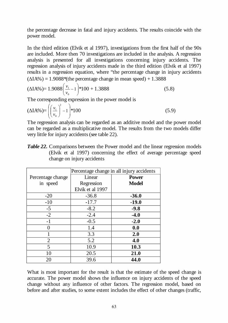
63

the percentage decrease in fatal and injury accidents. The results coincide with the power model. In the third edition (Elvik et al 1997), investigations from the first half of the 90s are included. More then 70 investigations are included in the analysis. A regression analysis is presented for all investigations concerning injury accidents. The regression analysis of injury accidents made in the third edition (Elvik et al 1997) results in a regression equation, where “the percentage change in injury accidents (∆IA%) = 1.9088*(the percentage change in mean speed) + 1.3888

(∆IA%)= 1.9088

−1

0

1

vv *100 + 1.3888 (5.8)

The corresponding expression in the power model is

(∆IA%)=

−

1

2

0

1

vv *100 (5.9)

The regression analysis can be regarded as an additive model and the power model can be regarded as a multiplicative model. The results from the two models differ very little for injury accidents (see table 22). Table 22. Comparisons between the Power model and the linear regression models

(Elvik et al 1997) concerning the effect of average percentage speed change on injury accidents

Percentage change in all injury accidents

Percentage change Linear Power in speed Regression Model

Elvik et al 1997 -20 -36.8 -36.0 -10 -17.7 -19.0 -5 -8.2 -9.8 -2 -2.4 -4.0 -1 -0.5 -2.0 0 1.4 0.0 1 3.3 2.0 2 5.2 4.0 5 10.9 10.3

10 20.5 21.0 20 39.6 44.0

What is most important for the result is that the estimate of the speed change is accurate. The power model shows the influence on injury accidents of the speed change without any influence of other factors. The regression model, based on before and after studies, to some extent includes the effect of other changes (traffic,

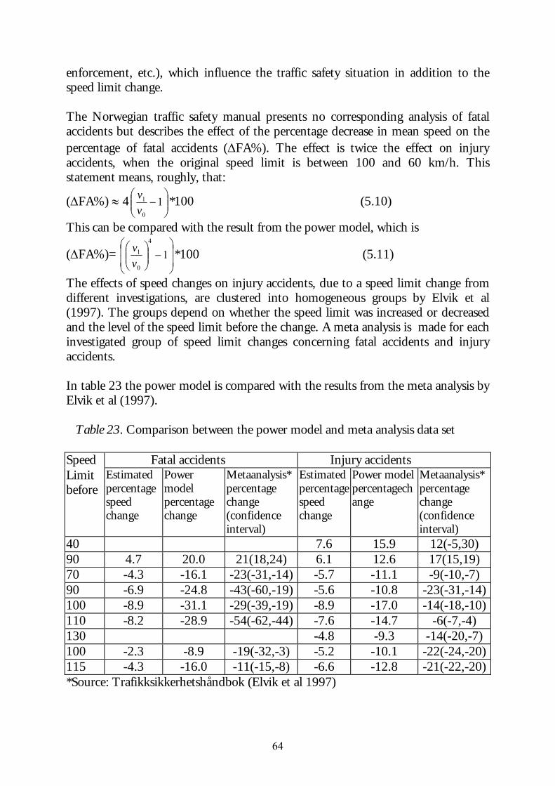
64

enforcement, etc.), which influence the traffic safety situation in addition to the speed limit change. The Norwegian traffic safety manual presents no corresponding analysis of fatal accidents but describes the effect of the percentage decrease in mean speed on the percentage of fatal accidents (∆FA%). The effect is twice the effect on injury accidents, when the original speed limit is between 100 and 60 km/h. This statement means, roughly, that:

(∆FA%) ≈ 4

−1

0

1

vv *100 (5.10)

This can be compared with the result from the power model, which is

(∆FA%)=

−

1

4

0

1

vv *100 (5.11)

The effects of speed changes on injury accidents, due to a speed limit change from different investigations, are clustered into homogeneous groups by Elvik et al (1997). The groups depend on whether the speed limit was increased or decreased and the level of the speed limit before the change. A meta analysis is made for each investigated group of speed limit changes concerning fatal accidents and injury accidents. In table 23 the power model is compared with the results from the meta analysis by Elvik et al (1997).

Table 23. Comparison between the power model and meta analysis data set

Speed Fatal accidents Injury accidents Limit before

Estimated percentage speed change

Power model percentage change

Metaanalysis* percentage change (confidence interval)

Estimated percentage speed change

Power model percentagechange

Metaanalysis* percentage change (confidence interval)

40 7.6 15.9 12(-5,30) 90 4.7 20.0 21(18,24) 6.1 12.6 17(15,19) 70 -4.3 -16.1 -23(-31,-14) -5.7 -11.1 -9(-10,-7) 90 -6.9 -24.8 -43(-60,-19) -5.6 -10.8 -23(-31,-14)100 -8.9 -31.1 -29(-39,-19) -8.9 -17.0 -14(-18,-10)110 -8.2 -28.9 -54(-62,-44) -7.6 -14.7 -6(-7,-4) 130 -4.8 -9.3 -14(-20,-7) 100 -2.3 -8.9 -19(-32,-3) -5.2 -10.1 -22(-24,-20)115 -4.3 -16.0 -11(-15,-8) -6.6 -12.8 -21(-22,-20)*Source: Trafikksikkerhetshåndbok (Elvik et al 1997)

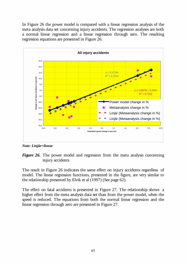
65

In Figure 26 the power model is compared with a linear regression analysis of the meta analysis data set concerning injury accidents. The regression analyses are both a normal linear regression and a linear regression through zero. The resulting regression equations are presented in Figure 26.

All injury accidents

y = 2,0073x - 2,2261R2 = 0,7252

y = 2,1726xR2 = 0,7053

-30,0

-25,0

-20,0

-15,0

-10,0

-5,0

0,0

5,0

10,0

15,0

20,0

25,0

-10,0 -8,0 -6,0 -4,0 -2,0 0,0 2,0 4,0 6,0 8,0 10,0

Estimated speed change in percent

Cha

nge

in a

ll in

jury

acc

iden

ts in

per

cent

Power model change in %Metaanalysis change in %Linjär (Metaanalysis change in %)Linjär (Metaanalysis change in %)

Note: Linjär=linear Figure 26. The power model and regression from the meta analysis concerning

injury accidents The result in Figure 26 indicates the same effect on injury accidents regardless of model. The linear regression functions, presented in the figure, are very similar to the relationship presented by Elvik et al (1997) (See page 62). The effect on fatal accidents is presented in Figure 27. The relationship shows a higher effect from the meta analysis data set than from the power model, when the speed is reduced. The equations from both the normal linear regression and the linear regression through zero are presented in Figure 27.

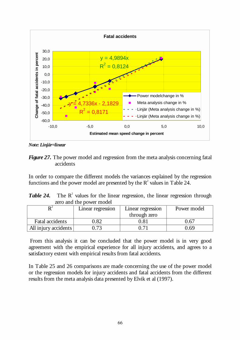
66

Fatal accidents

y = 4,9894xR2 = 0,8124

y = 4,7336x - 2,1829R2 = 0,8171

-60,0

-50,0

-40,0

-30,0

-20,0

-10,0

0,0

10,0

20,0

30,0

-10,0 -5,0 0,0 5,0 10,0

Estimated mean speed change in percent

Cha

nge

of fa

tal a

ccid

ents

in p

erce

nt

Power modelchange in %

Meta analysis change in %Linjär (Meta analysis change in %)

Linjär (Meta analysis change in %)

Note: Linjär=linear Figure 27. The power model and regression from the meta analysis concerning fatal

accidents In order to compare the different models the variances explained by the regression functions and the power model are presented by the R2 values in Table 24. Table 24. The R2 values for the linear regression, the linear regression through

zero and the power model R2 Linear regression Linear regression

through zero Power model

Fatal accidents 0.82 0.81 0.67 All injury accidents 0.73 0.71 0.69 From this analysis it can be concluded that the power model is in very good agreement with the empirical experience for all injury accidents, and agrees to a satisfactory extent with empirical results from fatal accidents. In Table 25 and 26 comparisons are made concerning the use of the power model or the regression models for injury accidents and fatal accidents from the different results from the meta analysis data presented by Elvik et al (1997).

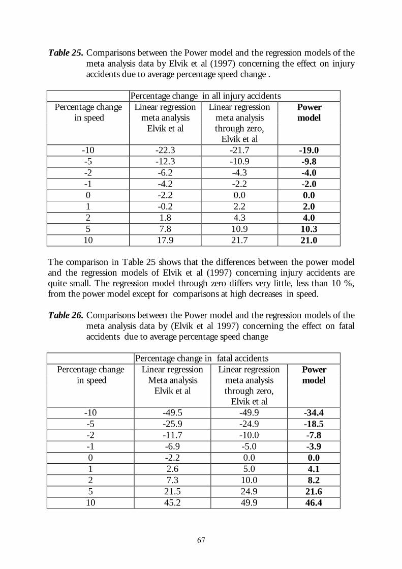
67

Table 25. Comparisons between the Power model and the regression models of the meta analysis data by Elvik et al (1997) concerning the effect on injury accidents due to average percentage speed change .

Percentage change in all injury accidents

Percentage change Linear regression Linear regression Power in speed meta analysis meta analysis model

Elvik et al through zero, Elvik et al

-10 -22.3 -21.7 -19.0 -5 -12.3 -10.9 -9.8 -2 -6.2 -4.3 -4.0 -1 -4.2 -2.2 -2.0 0 -2.2 0.0 0.0 1 -0.2 2.2 2.0 2 1.8 4.3 4.0 5 7.8 10.9 10.3

10 17.9 21.7 21.0 The comparison in Table 25 shows that the differences between the power model and the regression models of Elvik et al (1997) concerning injury accidents are quite small. The regression model through zero differs very little, less than 10 %, from the power model except for comparisons at high decreases in speed. Table 26. Comparisons between the Power model and the regression models of the

meta analysis data by (Elvik et al 1997) concerning the effect on fatal accidents due to average percentage speed change

Percentage change in fatal accidents

Percentage change Linear regression Linear regression Power in speed Meta analysis meta analysis model

Elvik et al through zero, Elvik et al

-10 -49.5 -49.9 -34.4 -5 -25.9 -24.9 -18.5 -2 -11.7 -10.0 -7.8 -1 -6.9 -5.0 -3.9 0 -2.2 0.0 0.0 1 2.6 5.0 4.1 2 7.3 10.0 8.2 5 21.5 24.9 21.6 10 45.2 49.9 46.4

68

The comparison in Table 26 and Figure 27 shows that the linear regression models will result in stronger effects on fatal accidents, when the speed decreases, compared with the power model. The power model is related to the change in kinetic energy and is symmetric multiplicatively and not additively as the regression model. Finland has experience of decreased speed limits during wintertime partly from a statistical experiment during two winter periods (1987/88 and 1988/89). A permanent reduction of the speed limit from 100 km/h to 80 km/h on large parts of the road network was introduced during the winter periods since 1989 and 1991. The results from the experiment coincide with the expected reduction based on the power model. In Finland a long-term study in 1987-1996 resulted in a higher decrease in injury accidents due to a general improvement in traffic safety. The twice higher effect on fatalities than on injured was also confirmed (Peltola 2000). There are very few accident investigations in urban areas of the changes in speed limits. One reason is that speed limits in urban areas have been unchanged or at 50 km/h for many years in a lot of countries. Some countries had the speed limit of 60 km/h in urban areas and changed it to 50 km/h during the last decades. One of these countries is Denmark. The speed limit was lowered from 60 km/h to 50 km/h in 1985. (Engel 1988). The result corresponds to the power model and the estimated decrease in number of injured was 9 % and the decrease in the number of fatalities was 24 %. The estimated speed reduction was 4-6 %. The predicted values from the power model are then a decrease of 10 % in injury accidents and a 20 % reduction in the number of fatalities. In 1990 speed zones of 20 miles per hour instead of 30 miles per hour were introduced in the UK. A before and after investigation shows a speed reduction of 37 % and a reduction of the injury accident risk with 58 %. The corresponding value of the power model is 60 %. Even for fatalities the empirical result corresponds to the power model (Webster & Mackie 1996). It is difficult to estimate representative speed or speed changes in urban areas due to the variation of speed in space compared with rural areas. But relative speed changes seem to be of the same magnitude regardless of the method used for speed measurement, for example space mean speed between intersections or travel speed for the section.

69

5.6 Validation of the power model based on cross-sectional data 5.6.1 Injury accident rate The effects of changed speeds on safety presented in the previous chapters can also be verified in a cross-sectional analysis. Some attempts have been made before (Nilsson 1984 b) and recently (Carlsson 2002, Taylor et al 2002) and the conclusions are the same concerning the relationships between safety and speeds as in the before and after investigations. The difficulties are to eliminate or control for the differences between the investigated environments which influence the safety situation in addition to the difference in speed between different environments. This can be done concerning the accident consequences but is more difficult concerning the injury accident rate or fatal accident rate. The injury accident consequences are more or less dependent on the speed situation and the distribution of accident types. The accident rates, however, can depend on a lot of different factors, which are difficult to control. In before and after investigations of speed (limit) changes these factors are regarded as the same between the periods or controlled for between the periods. In a cross-sectional study of the dependence of the injury accident rate on speeds, the effect of other factors than speed or speed limit such as traffic and road environment should be similar on all sections. If this is the case, the variation in safety will mainly be a result of the differences in speed. The ultimate situation is to compare the accident rate situation on road sections where the only difference is the speed (limit) during the same time period. This is to a high degree the situation in the following investigation. During 1997 the SNRA (Swedish National Road Administration) registered the mean speed on more than 100 road sections on two-lane roads with the road width of 13 metres. 62 road sections had the speed limit of 110 km/h and 43 road sections had the speed limit of 90 km/h. Accident data was collected for the period 1991-1997. The accident data was supplemented in order to present the number of fatalities, severely and slightly injured in fatal accidents, the number of severely and slightly injured in serious injury accidents and also the number of slightly injured in slight injury accidents (see Table 27). In this way it was possible to illustrate both the accident and the injury situation. The estimate of the average speed for each group of sections is based on several road sections with about the same average speed. The road sections had not been reconstructed since 1991.

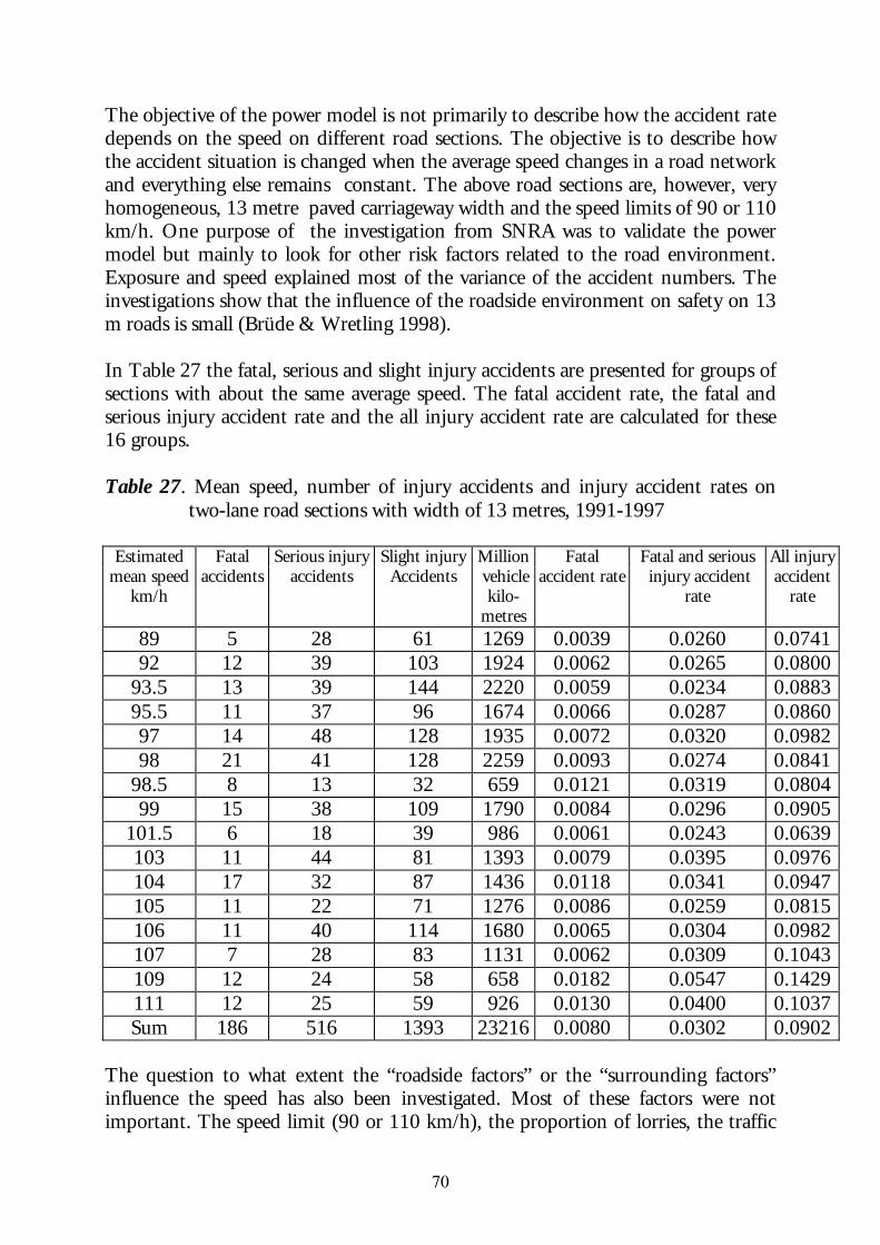
70

The objective of the power model is not primarily to describe how the accident rate depends on the speed on different road sections. The objective is to describe how the accident situation is changed when the average speed changes in a road network and everything else remains constant. The above road sections are, however, very homogeneous, 13 metre paved carriageway width and the speed limits of 90 or 110 km/h. One purpose of the investigation from SNRA was to validate the power model but mainly to look for other risk factors related to the road environment. Exposure and speed explained most of the variance of the accident numbers. The investigations show that the influence of the roadside environment on safety on 13 m roads is small (Brüde & Wretling 1998). In Table 27 the fatal, serious and slight injury accidents are presented for groups of sections with about the same average speed. The fatal accident rate, the fatal and serious injury accident rate and the all injury accident rate are calculated for these 16 groups. Table 27. Mean speed, number of injury accidents and injury accident rates on

two-lane road sections with width of 13 metres, 1991-1997

Estimated Fatal Serious injury Slight injury Million Fatal Fatal and serious All injurymean speed

km/h accidents accidents Accidents vehicle

kilo-metres

accident rate injury accident rate

accident rate

89 5 28 61 1269 0.0039 0.0260 0.074192 12 39 103 1924 0.0062 0.0265 0.0800

93.5 13 39 144 2220 0.0059 0.0234 0.088395.5 11 37 96 1674 0.0066 0.0287 0.086097 14 48 128 1935 0.0072 0.0320 0.098298 21 41 128 2259 0.0093 0.0274 0.0841

98.5 8 13 32 659 0.0121 0.0319 0.080499 15 38 109 1790 0.0084 0.0296 0.0905

101.5 6 18 39 986 0.0061 0.0243 0.0639103 11 44 81 1393 0.0079 0.0395 0.0976104 17 32 87 1436 0.0118 0.0341 0.0947105 11 22 71 1276 0.0086 0.0259 0.0815106 11 40 114 1680 0.0065 0.0304 0.0982107 7 28 83 1131 0.0062 0.0309 0.1043109 12 24 58 658 0.0182 0.0547 0.1429111 12 25 59 926 0.0130 0.0400 0.1037Sum 186 516 1393 23216 0.0080 0.0302 0.0902

The question to what extent the “roadside factors” or the “surrounding factors” influence the speed has also been investigated. Most of these factors were not important. The speed limit (90 or 110 km/h), the proportion of lorries, the traffic

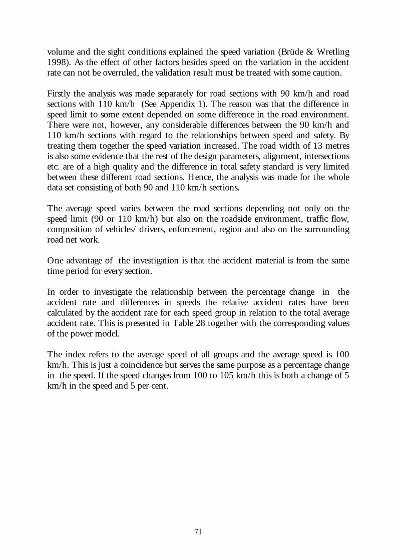
71

volume and the sight conditions explained the speed variation (Brüde & Wretling 1998). As the effect of other factors besides speed on the variation in the accident rate can not be overruled, the validation result must be treated with some caution. Firstly the analysis was made separately for road sections with 90 km/h and road sections with 110 km/h (See Appendix 1). The reason was that the difference in speed limit to some extent depended on some difference in the road environment. There were not, however, any considerable differences between the 90 km/h and 110 km/h sections with regard to the relationships between speed and safety. By treating them together the speed variation increased. The road width of 13 metres is also some evidence that the rest of the design parameters, alignment, intersections etc. are of a high quality and the difference in total safety standard is very limited between these different road sections. Hence, the analysis was made for the whole data set consisting of both 90 and 110 km/h sections. The average speed varies between the road sections depending not only on the speed limit (90 or 110 km/h) but also on the roadside environment, traffic flow, composition of vehicles/ drivers, enforcement, region and also on the surrounding road net work. One advantage of the investigation is that the accident material is from the same time period for every section. In order to investigate the relationship between the percentage change in the accident rate and differences in speeds the relative accident rates have been calculated by the accident rate for each speed group in relation to the total average accident rate. This is presented in Table 28 together with the corresponding values of the power model. The index refers to the average speed of all groups and the average speed is 100 km/h. This is just a coincidence but serves the same purpose as a percentage change in the speed. If the speed changes from 100 to 105 km/h this is both a change of 5 km/h in the speed and 5 per cent.

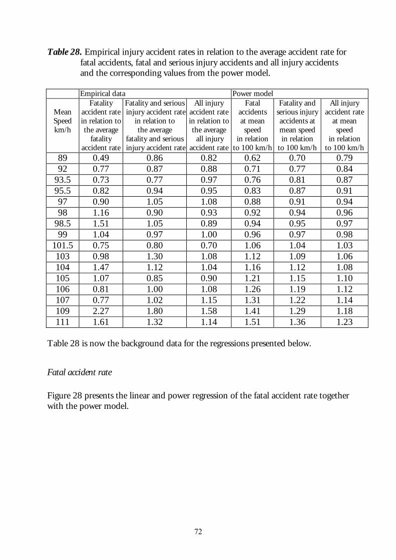
72

Table 28. Empirical injury accident rates in relation to the average accident rate for fatal accidents, fatal and serious injury accidents and all injury accidents and the corresponding values from the power model.

Empirical data Power model

Fatality Fatality and serious All injury Fatal Fatality and All injury Mean accident rate injury accident rate accident rate accidents serious injury accident rateSpeed in relation to in relation to in relation to at mean accidents at at mean km/h the average the average the average speed mean speed speed

fatality fatality and serious all injury in relation in relation in relation accident rate injury accident rate accident rate to 100 km/h to 100 km/h to 100 km/h

89 0.49 0.86 0.82 0.62 0.70 0.79 92 0.77 0.87 0.88 0.71 0.77 0.84

93.5 0.73 0.77 0.97 0.76 0.81 0.87 95.5 0.82 0.94 0.95 0.83 0.87 0.91 97 0.90 1.05 1.08 0.88 0.91 0.94 98 1.16 0.90 0.93 0.92 0.94 0.96

98.5 1.51 1.05 0.89 0.94 0.95 0.97 99 1.04 0.97 1.00 0.96 0.97 0.98

101.5 0.75 0.80 0.70 1.06 1.04 1.03 103 0.98 1.30 1.08 1.12 1.09 1.06 104 1.47 1.12 1.04 1.16 1.12 1.08 105 1.07 0.85 0.90 1.21 1.15 1.10 106 0.81 1.00 1.08 1.26 1.19 1.12 107 0.77 1.02 1.15 1.31 1.22 1.14 109 2.27 1.80 1.58 1.41 1.29 1.18 111 1.61 1.32 1.14 1.51 1.36 1.23

Table 28 is now the background data for the regressions presented below.

Fatal accident rate Figure 28 presents the linear and power regression of the fatal accident rate together with the power model.

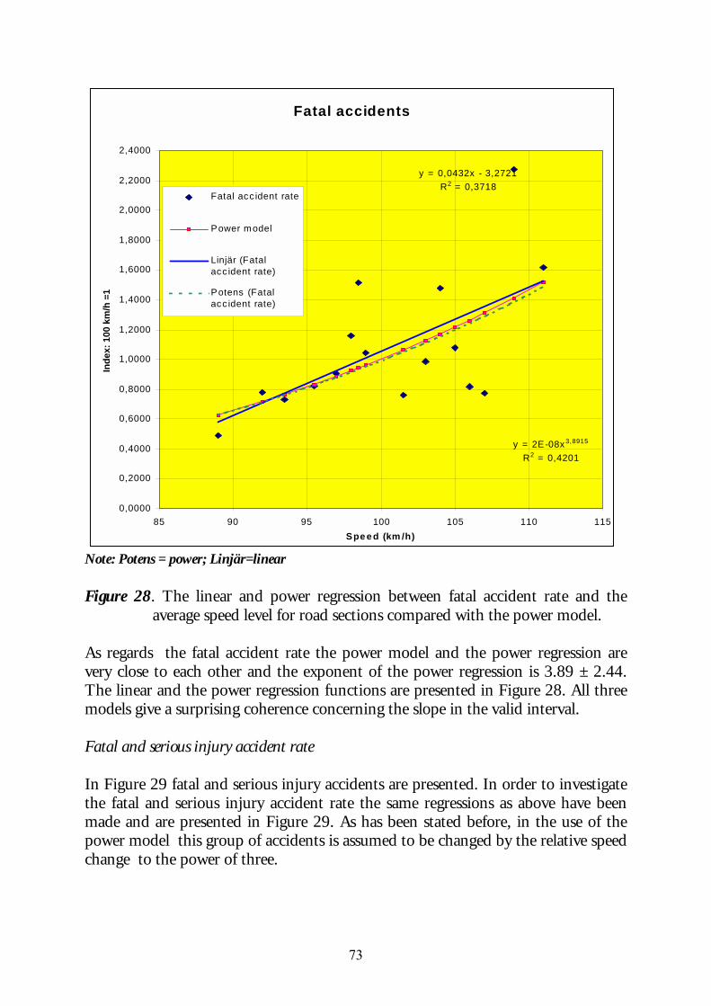
73

Fatal accidents

y = 0,0432x - 3,2721R2 = 0,3718

y = 2E-08x3,8915

R2 = 0,4201

0,0000

0,2000

0,4000

0,6000

0,8000

1,0000

1,2000

1,4000

1,6000

1,8000

2,0000

2,2000

2,4000

85 90 95 100 105 110 115Spe e d (km /h)

Inde

x: 1

00 k

m/h

=1

Fatal acc ident rate

Power model

Linjär (Fatalacc ident rate)

Potens (Fatalacc ident rate)

Note: Potens = power; Linjär=linear Figure 28. The linear and power regression between fatal accident rate and the

average speed level for road sections compared with the power model. As regards the fatal accident rate the power model and the power regression are very close to each other and the exponent of the power regression is 3.89 ± 2.44. The linear and the power regression functions are presented in Figure 28. All three models give a surprising coherence concerning the slope in the valid interval. Fatal and serious injury accident rate In Figure 29 fatal and serious injury accidents are presented. In order to investigate the fatal and serious injury accident rate the same regressions as above have been made and are presented in Figure 29. As has been stated before, in the use of the power model this group of accidents is assumed to be changed by the relative speed change to the power of three.

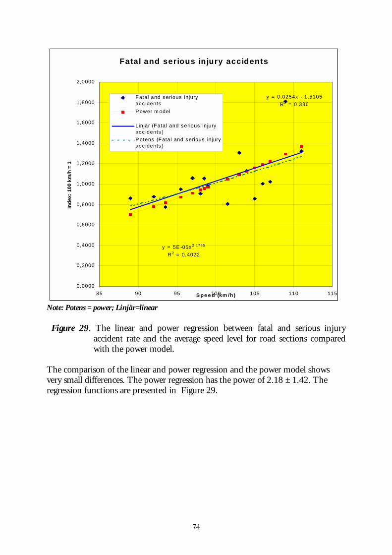
74

Fatal and serious injury accidents

y = 0,0254x - 1,5105R2 = 0,386

y = 5E -05x 2,1755

R2 = 0,4022

0,0000

0,2000

0,4000

0,6000

0,8000

1,0000

1,2000

1,4000

1,6000

1,8000

2,0000

85 90 95 100 105 110 115S pe e d (km /h)

Inde

x: 1

00 k

m/h

= 1

Fatal and serious injuryacc identsP ower m odel

Linjär (Fatal and serious injuryacc idents )P otens (Fatal and serious injuryacc idents )

Note: Potens = power; Linjär=linear Figure 29. The linear and power regression between fatal and serious injury

accident rate and the average speed level for road sections compared with the power model.

The comparison of the linear and power regression and the power model shows very small differences. The power regression has the power of 2.18 ± 1.42. The regression functions are presented in Figure 29.

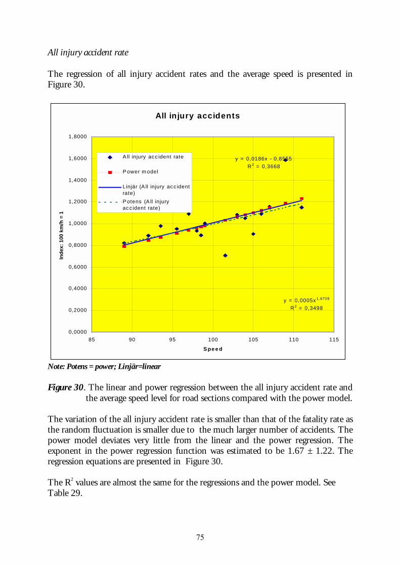
75

All injury accident rate The regression of all injury accident rates and the average speed is presented in Figure 30.

All injury accidents

y = 0,0186x - 0,8555R2 = 0,3668

y = 0,0005x 1,6705

R2 = 0,3498

0,0000

0,2000

0,4000

0,6000

0,8000

1,0000

1,2000

1,4000

1,6000

1,8000

85 90 95 100 105 110 115

S pe e d

Inde

x: 1

00 k

m/h

= 1

A ll injury acc ident rate

P ower m odel

Linjär (A ll injury acc identrate)P otens (A ll injuryacc ident rate)

Note: Potens = power; Linjär=linear Figure 30. The linear and power regression between the all injury accident rate and

the average speed level for road sections compared with the power model. The variation of the all injury accident rate is smaller than that of the fatality rate as the random fluctuation is smaller due to the much larger number of accidents. The power model deviates very little from the linear and the power regression. The exponent in the power regression function was estimated to be 1.67 ± 1.22. The regression equations are presented in Figure 30. The R2 values are almost the same for the regressions and the power model. See Table 29.

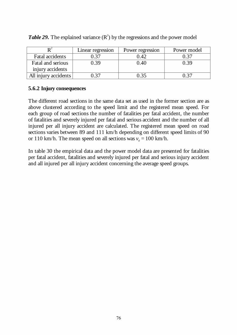
76

Table 29. The explained variance (R2) by the regressions and the power model

R2 Linear regression Power regression Power model Fatal accidents 0.37 0.42 0.37

Fatal and serious injury accidents

0.39 0.40 0.39

All injury accidents 0.37 0.35 0.37

5.6.2 Injury consequences The different road sections in the same data set as used in the former section are as above clustered according to the speed limit and the registered mean speed. For each group of road sections the number of fatalities per fatal accident, the number of fatalities and severely injured per fatal and serious accident and the number of all injured per all injury accident are calculated. The registered mean speed on road sections varies between 89 and 111 km/h depending on different speed limits of 90 or 110 km/h. The mean speed on all sections was v0 = 100 km/h. In table 30 the empirical data and the power model data are presented for fatalities per fatal accident, fatalities and severely injured per fatal and serious injury accident and all injured per all injury accident concerning the average speed groups.

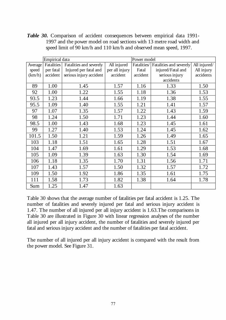
77

Table 30. Comparison of accident consequences between empirical data 1991-

1997 and the power model on road sections with 13 metre road width and speed limit of 90 km/h and 110 km/h and observed mean speed, 1997.

Empirical data Power model

Average Fatalities Fatalities and severely All injured Fatalities/ Fatalities and severely All injured/speed per fatal Injured per fatal and per all injury Fatal injured/Fatal and All injury

(km/h) accident serious injury accident accident accident serious injury accidents

accidents

89 1.00 1.45 1.57 1.16 1.33 1.50 92 1.00 1.22 1.55 1.18 1.36 1.53

93.5 1.23 1.44 1.66 1.19 1.38 1.55 95.5 1.09 1.40 1.55 1.21 1.41 1.57 97 1.07 1.35 1.57 1.22 1.43 1.59 98 1.24 1.50 1.71 1.23 1.44 1.60

98.5 1.00 1.43 1.68 1.23 1.45 1.61 99 1.27 1.40 1.53 1.24 1.45 1.62

101.5 1.50 1.21 1.59 1.26 1.49 1.65 103 1.18 1.51 1.65 1.28 1.51 1.67 104 1.47 1.69 1.61 1.29 1.53 1.68 105 1.09 1.39 1.63 1.30 1.54 1.69 106 1.18 1.35 1.70 1.31 1.56 1.71 107 1.43 1.57 1.50 1.32 1.57 1.72 109 1.50 1.92 1.86 1.35 1.61 1.75 111 1.58 1.73 1.82 1.38 1.64 1.78 Sum 1.25 1.47 1.63

Table 30 shows that the average number of fatalities per fatal accident is 1.25. The number of fatalities and severely injured per fatal and serious injury accident is 1.47. The number of all injured per all injury accident is 1.63.The comparisons in Table 30 are illustrated in Figure 30 with linear regression analyses of the number all injured per all injury accident, the number of fatalities and severely injured per fatal and serious injury accident and the number of fatalities per fatal accident. The number of all injured per all injury accident is compared with the result from the power model. See Figure 31.

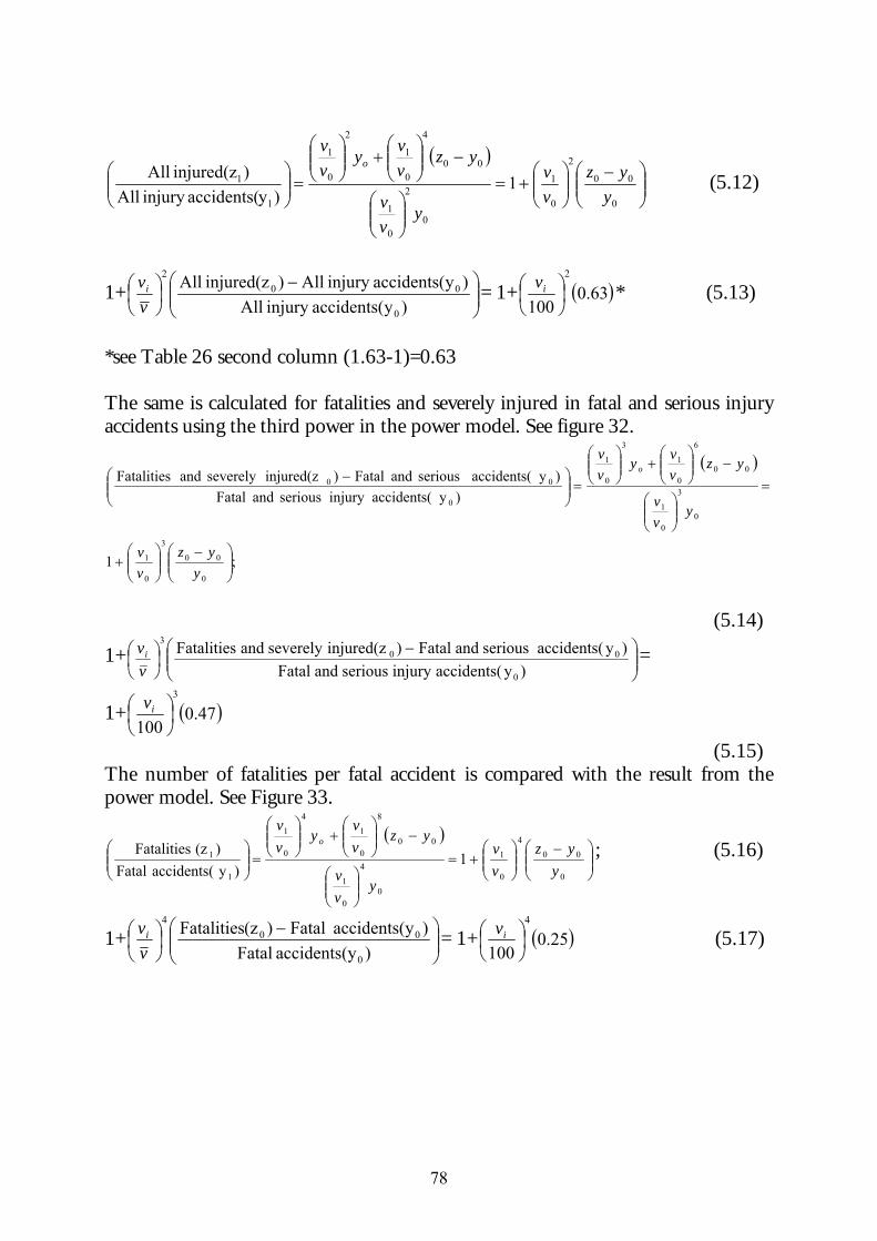
78

( )

−

+=

−

+

=

0

00

2

0

1

0

2

0

1

00

4

0

1

2

0

1

1

1 1)yaccidents(injury All

)injured(z Ally

yzvv

yvv

yzvvy

vv

o

(5.12)

1+

−

)yaccidents(injury All)yaccidents(injury All)injured(z All

0

002

vvi = 1+ ( )63.0

100

2

iv * (5.13)

*see Table 26 second column (1.63-1)=0.63 The same is calculated for fatalities and severely injured in fatal and serious injury accidents using the third power in the power model. See figure 32.

( )

;1

)yaccidents(injury serious and Fatal)yaccidents( serious and Fatal )injured(zseverely and Fatalities

0

00

3

0

1

0

3

0

1

00

6

0

1

3

0

1

0

00

−

+

=

−

+

=

−

yyz

vv

yvv

yzvvy

vv

o

(5.14)

1+

−

)yaccidents(injury serious and Fatal)yaccidents( serious and Fatal )injured(zseverely and Fatalities

0

003

vvi =

1+ ( )47.0100

3

iv

(5.15) The number of fatalities per fatal accident is compared with the result from the power model. See Figure 33.

( )

−

+=

−

+

=

0

004

0

1

0

4

0

1

00

8

0

1

4

0

1

1

1 1)yaccidents( Fatal

)(zFatalitiesy

yzvv

yvv

yzvv

yvv

o; (5.16)

1+

−

)yaccidents( Fatal)yaccidents( Fatal )(zFatalities

0

004

vvi = 1+ ( )25.0

100

4

iv (5.17)

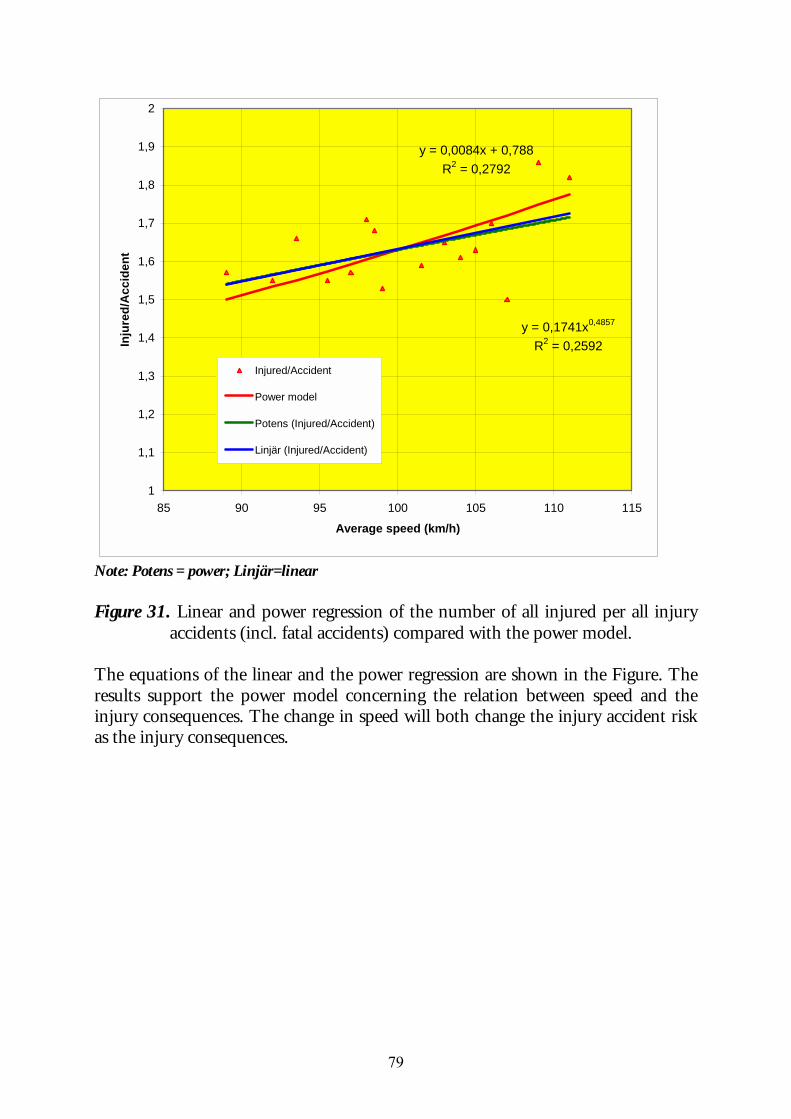
79

y = 0,1741x0,4857

R2 = 0,2592

y = 0,0084x + 0,788R2 = 0,2792

1

1,1

1,2

1,3

1,4

1,5

1,6

1,7

1,8

1,9

2

85 90 95 100 105 110 115

Average speed (km/h)

Inju

red/

Acc

iden

t

Injured/Accident

Power model

Potens (Injured/Accident)

Linjär (Injured/Accident)

Note: Potens = power; Linjär=linear Figure 31. Linear and power regression of the number of all injured per all injury

accidents (incl. fatal accidents) compared with the power model. The equations of the linear and the power regression are shown in the Figure. The results support the power model concerning the relation between speed and the injury consequences. The change in speed will both change the injury accident risk as the injury consequences.

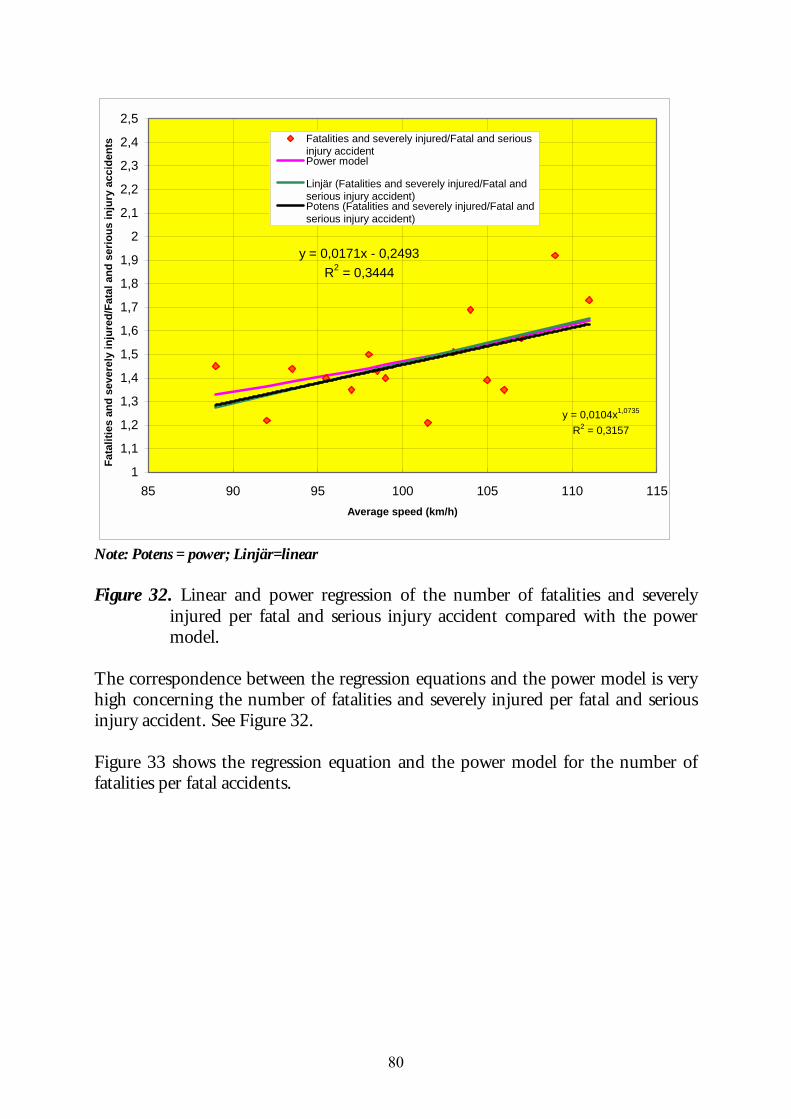
80

y = 0,0171x - 0,2493R2 = 0,3444

y = 0,0104x1,0735

R2 = 0,3157

1

1,1

1,2

1,3

1,4

1,5

1,6

1,7

1,8

1,9

2

2,1

2,2

2,3

2,4

2,5

85 90 95 100 105 110 115Average speed (km/h)

Fata

litie

s an

d se

vere

ly in

jure

d/Fa

tal a

nd s

erio

us in

jury

acc

iden

ts Fatalities and severely injured/Fatal and serious

injury accidentPower model

Linjär (Fatalities and severely injured/Fatal andserious injury accident)Potens (Fatalities and severely injured/Fatal andserious injury accident)

Note: Potens = power; Linjär=linear Figure 32. Linear and power regression of the number of fatalities and severely

injured per fatal and serious injury accident compared with the power model.

The correspondence between the regression equations and the power model is very high concerning the number of fatalities and severely injured per fatal and serious injury accident. See Figure 32. Figure 33 shows the regression equation and the power model for the number of fatalities per fatal accidents.

81

y = 0,0004x1,7638

R2 = 0,51

y = 0,0223x - 1,0046R2 = 0,5137

1

1,1

1,2

1,3

1,4

1,5

1,6

1,7

85 90 95 100 105 110 115

Average speed (km/h)

Fata

litie

s/Fa

tal a

ccid

ents

Fatalities/Fatal accident

Power model

Potens (Fatalities/Fatalaccident)

Linjär (Fatalities/Fatalaccident)

Note: Potens = power; Linjär=linear Figure 33. Linear and power regression of the number of fatalities per fatal accident

compared with the power model. In all cases in Figure 31, 32 and 33 the number of all injured per all injury accident, the number of fatalities and severely injured per fatal and serious injury accident and the number of fatalities per fatal accident increase with speed and the increase corresponds in general with the power model. The empirical data of fatalities per fatal accident, however, shows a stronger relationship with speed than the power model. The ratio between fatalities and fatal accidents, however, varies a lot depending on the small numbers. Table 31 describes into what degree the linear and power regressions and the power model explain the variance. The regression line of the linear regression and the power regression coincide. The power regression is also made for the f(x) –1 (Table 31) to validate the exponents of the power model. The power regression exponents are presented for “All injured/All injury accidents” and for “Fatalities and severely injured/Fatal and serious injury accidents". The corresponding power regression exponent for Fatalities/Fatal accidents cannot be calculated as some of the empirical values are 1.0 and became zero, which is not acceptable in the power regression. Therefore the zero values have been modified.

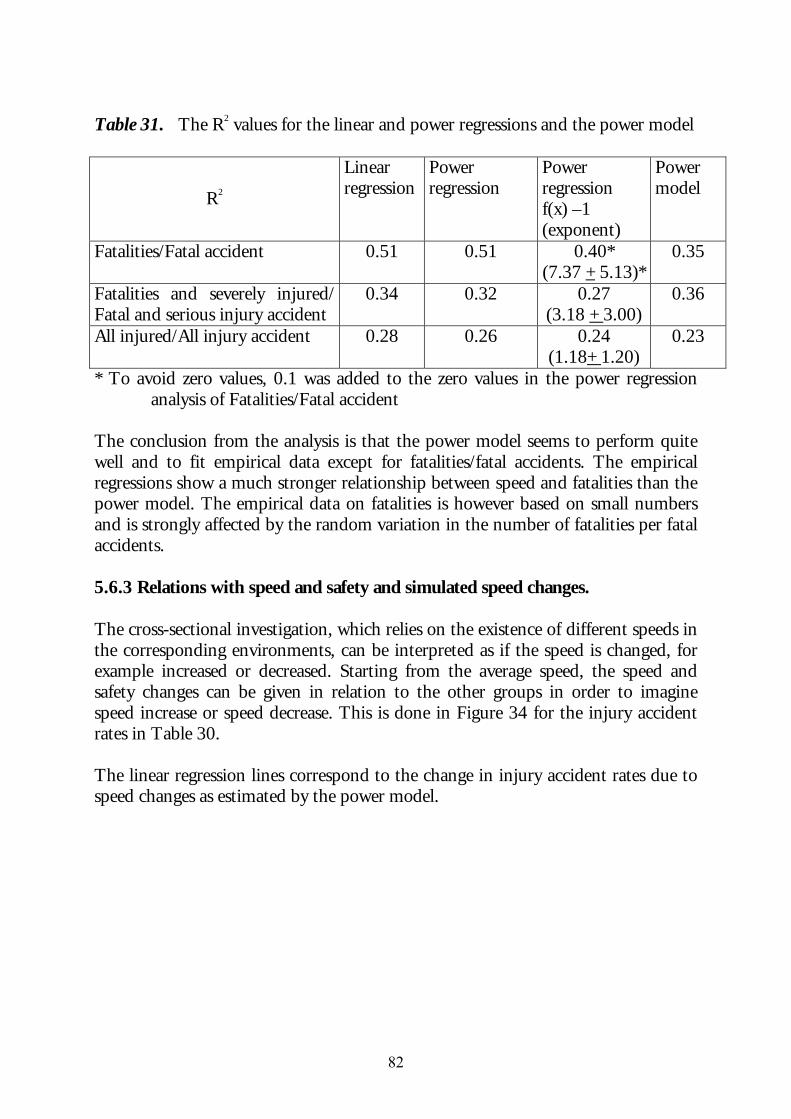
82

Table 31. The R2 values for the linear and power regressions and the power model

R2

Linear regression

Power regression

Power regression f(x) –1 (exponent)

Power model

Fatalities/Fatal accident 0.51 0.51 0.40* (7.37 + 5.13)*

0.35

Fatalities and severely injured/ Fatal and serious injury accident

0.34 0.32 0.27 (3.18 + 3.00)

0.36

All injured/All injury accident 0.28 0.26 0.24 (1.18+ 1.20)

0.23

* To avoid zero values, 0.1 was added to the zero values in the power regression analysis of Fatalities/Fatal accident

The conclusion from the analysis is that the power model seems to perform quite well and to fit empirical data except for fatalities/fatal accidents. The empirical regressions show a much stronger relationship between speed and fatalities than the power model. The empirical data on fatalities is however based on small numbers and is strongly affected by the random variation in the number of fatalities per fatal accidents. 5.6.3 Relations with speed and safety and simulated speed changes. The cross-sectional investigation, which relies on the existence of different speeds in the corresponding environments, can be interpreted as if the speed is changed, for example increased or decreased. Starting from the average speed, the speed and safety changes can be given in relation to the other groups in order to imagine speed increase or speed decrease. This is done in Figure 34 for the injury accident rates in Table 30. The linear regression lines correspond to the change in injury accident rates due to speed changes as estimated by the power model.

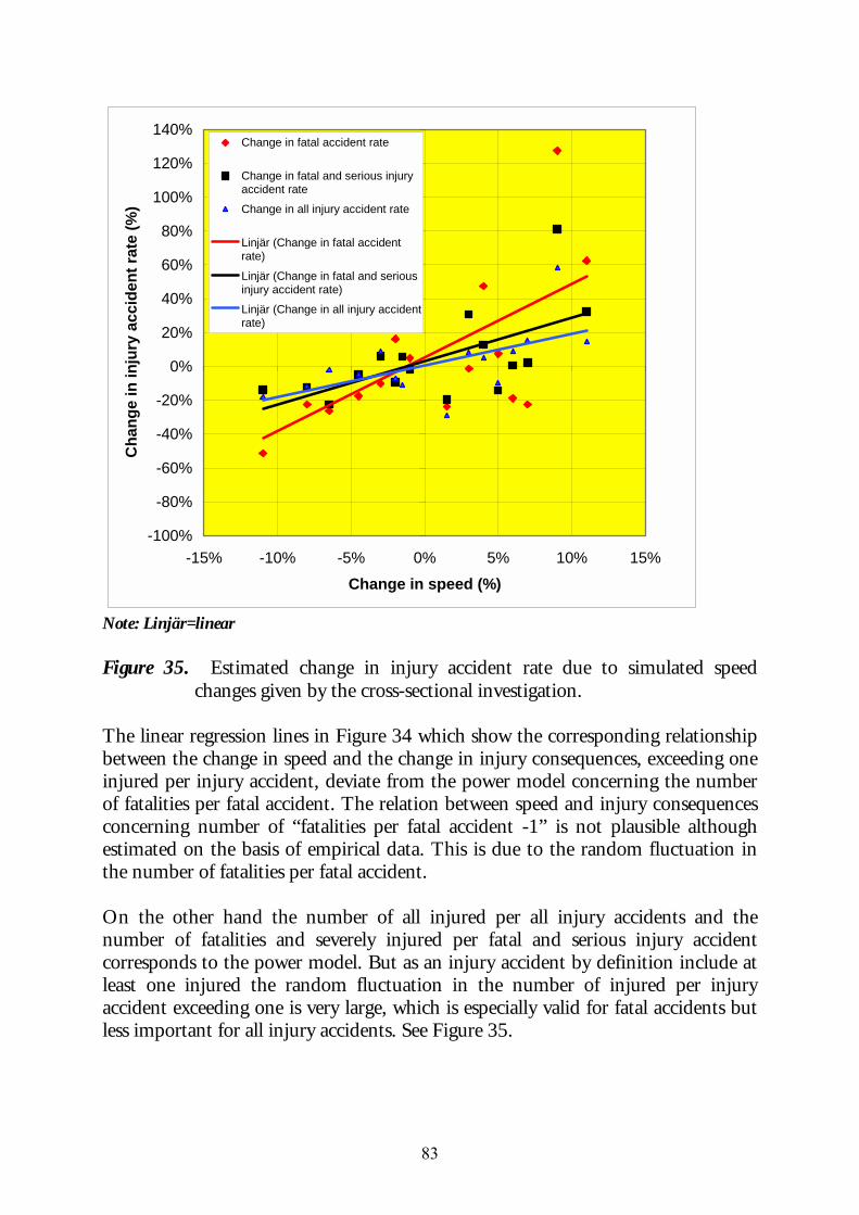
83

-100%

-80%

-60%

-40%

-20%

0%

20%

40%

60%

80%

100%

120%

140%

-15% -10% -5% 0% 5% 10% 15%

Change in speed (%)

Cha

nge

in in

jury

acc

iden

t rat

e (%

)Change in fatal accident rate

Change in fatal and serious injuryaccident rate

Change in all injury accident rate

Linjär (Change in fatal accidentrate)

Linjär (Change in fatal and seriousinjury accident rate)

Linjär (Change in all injury accidentrate)

Note: Linjär=linear Figure 35. Estimated change in injury accident rate due to simulated speed

changes given by the cross-sectional investigation. The linear regression lines in Figure 34 which show the corresponding relationship between the change in speed and the change in injury consequences, exceeding one injured per injury accident, deviate from the power model concerning the number of fatalities per fatal accident. The relation between speed and injury consequences concerning number of “fatalities per fatal accident -1” is not plausible although estimated on the basis of empirical data. This is due to the random fluctuation in the number of fatalities per fatal accident. On the other hand the number of all injured per all injury accidents and the number of fatalities and severely injured per fatal and serious injury accident corresponds to the power model. But as an injury accident by definition include at least one injured the random fluctuation in the number of injured per injury accident exceeding one is very large, which is especially valid for fatal accidents but less important for all injury accidents. See Figure 35.

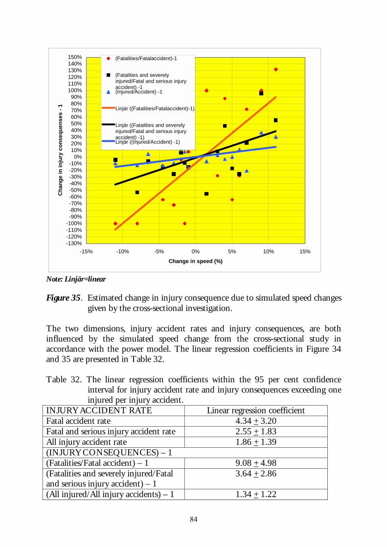
84

-130%-120%-110%-100%-90%-80%-70%-60%-50%-40%-30%-20%-10%

0%10%20%30%40%50%60%70%80%90%

100%110%120%130%140%150%

-15% -10% -5% 0% 5% 10% 15%

Change in speed (%)

Cha

nge

in in

jury

con

sequ

ense

s - 1

(Fatalities/Fatalaccident)-1

(Fatalities and severelyinjured/Fatal and serious injuryaccident) -1(Injured/Accident) -1

Linjär ((Fatalities/Fatalaccident)-1)

Linjär ((Fatalities and severelyinjured/Fatal and serious injuryaccident) -1)Linjär ((Injured/Accident) -1)

Note: Linjär=linear Figure 35. Estimated change in injury consequence due to simulated speed changes

given by the cross-sectional investigation. The two dimensions, injury accident rates and injury consequences, are both influenced by the simulated speed change from the cross-sectional study in accordance with the power model. The linear regression coefficients in Figure 34 and 35 are presented in Table 32. Table 32. The linear regression coefficients within the 95 per cent confidence

interval for injury accident rate and injury consequences exceeding one injured per injury accident.

INJURY ACCIDENT RATE Linear regression coefficient Fatal accident rate 4.34 + 3.20 Fatal and serious injury accident rate 2.55 + 1.83 All injury accident rate 1.86 + 1.39 (INJURY CONSEQUENCES) – 1 (Fatalities/Fatal accident) – 1 9.08 + 4.98 (Fatalities and severely injured/Fatal and serious injury accident) – 1

3.64 + 2.86

(All injured/All injury accidents) – 1 1.34 + 1.22

85

As the intercept does not differ from zero, the linear coefficients are close to the coefficients in the power model both for injury accident rates and for injury consequences in view of the fact that, by definition, at least one person is injured in an injury accident. Of course, before and after studies of speed changes through changed speed limits speed give of a more direct result. The disadvantages are that the before and after periods are normally too short and other measures introduced in the after period influence the result. Speed changes through changed general speed limits are rare but over the years the experience of the relation between speed level and safety has been very unanimous. There is some confusion about how the effect is expressed, by accidents or casualties, and how the exposure corresponds to the before and after period. The latter is easier in cross-sectional studies as the time period can be chosen. On the other hand cross-sectional studies are dependent on the coincidence that a group of roads have different speeds or speed limits but are the same in all other aspects which influence safety. 5.7 Use of the model The model was originally presented by me (Nilsson 1981) and has been presented on different occasions when the relationship between speed changes and safety has been analysed. This section presents both the background of the model, the use of the model (Evans 1991, Kallberg 1998, Frith 2000, Elvik 2000) and the calculation possibilities (OECD 1997 b). The primary objective of the model is to describe the effect of changed vehicle speeds on the number of accidents and the accident consequences on a macro level, a road network. The influence of the exposure is not treated inside the model and must be taken into account separately. The same is valid for any measure which is introduced at the same time as the vehicle speeds are changed. The model estimates the expected safety effect of the changes in speed on the number of injury accidents on a given road network and during a defined time period. The additional information needed is the average speed level of the motor vehicles during the same period. The model can then estimate - the change in the number of injury and fatal accidents as well as the number of

persons injured or fatalities if the average vehicle speed has been or is changed as a forecasting method

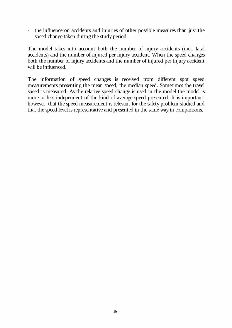
86

- the influence on accidents and injuries of other possible measures than just the speed change taken during the study period.

The model takes into account both the number of injury accidents (incl. fatal accidents) and the number of injured per injury accident. When the speed changes both the number of injury accidents and the number of injured per injury accident will be influenced. The information of speed changes is received from different spot speed measurements presenting the mean speed, the median speed. Sometimes the travel speed is measured. As the relative speed change is used in the model the model is more or less independent of the kind of average speed presented. It is important, however, that the speed measurement is relevant for the safety problem studied and that the speed level is representative and presented in the same way in comparisons.

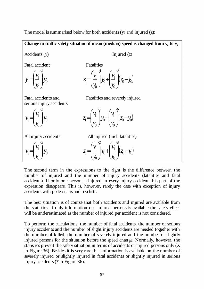
87

The model is summarised below for both accidents (y) and injured (z): Change in traffic safety situation if mean (median) speed is changed from v0 to v1

Accidents (y) Injured (z) Fatal accident Fatalities

0

4

0

11 y

vvy

=

( )00

8

0

10

4

0

11 yz

vvy

vvz −

+

=

Fatal accidents and Fatalities and severely injured serious injury accidents

0

3

0

11 y

vvy

=

( )00

6

0

10

3

0

11 yz

vvy

vvz −

+

=

All injury accidents All injured (incl. fatalities)

0

2

0

11 y

vvy

=

( )00

4

0

10

2

0

11 yz

vvy

vvz −

+

=

The second term in the expressions to the right is the difference between the number of injured and the number of injury accidents (fatalities and fatal accidents). If only one person is injured in every injury accident this part of the expression disappears. This is, however, rarely the case with exception of injury accidents with pedestrians and cyclists. The best situation is of course that both accidents and injured are available from the statistics. If only information on injured persons is available the safety effect will be underestimated as the number of injured per accident is not considered. To perform the calculations, the number of fatal accidents, the number of serious injury accidents and the number of slight injury accidents are needed together with the number of killed, the number of severely injured and the number of slightly injured persons for the situation before the speed change. Normally, however, the statistics present the safety situation in terms of accidents or injured persons only (X in Figure 36). Besides it is very rare that information is available on the number of severely injured or slightly injured in fatal accidents or slightly injured in serious injury accidents (* in Figure 36).

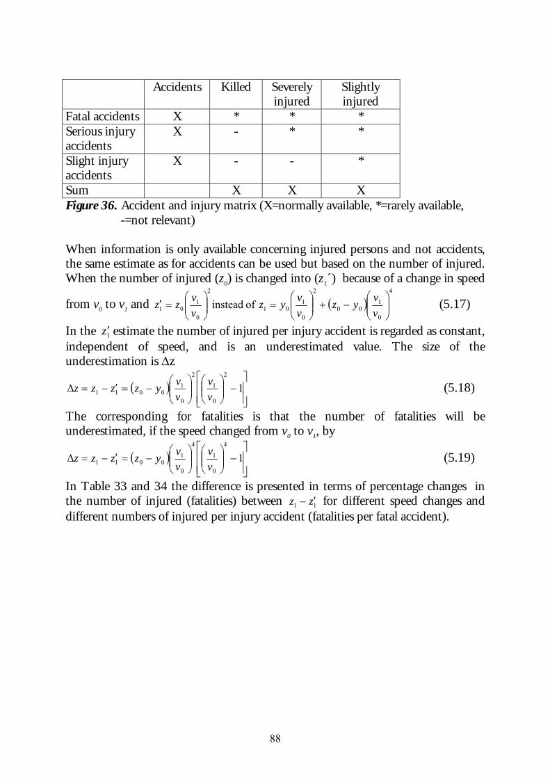
88

Accidents Killed Severely

injured Slightly injured

Fatal accidents X * * * Serious injury accidents

X - * *

Slight injury accidents

X - - *

Sum X X X Figure 36. Accident and injury matrix (X=normally available, *=rarely available, -=not relevant) When information is only available concerning injured persons and not accidents, the same estimate as for accidents can be used but based on the number of injured. When the number of injured (z0) is changed into (z1´) because of a change in speed

from v0 to v1 and ( )4

0

100

2

0

101

2

0

101 of instead

−+

=

=′

vvyz

vvyz

vvzz (5.17)

In the 1z ′ estimate the number of injured per injury accident is regarded as constant, independent of speed, and is an underestimated value. The size of the underestimation is ∆z

( )

−

−=′−= 1∆

2

0

1

2

0

10011 v

vvvyzzzz (5.18)

The corresponding for fatalities is that the number of fatalities will be underestimated, if the speed changed from v0 to v1, by

( )

−

−=′−= 1∆

4

0

1

4

0

10011 v

vvvyzzzz (5.19)

In Table 33 and 34 the difference is presented in terms of percentage changes in the number of injured (fatalities) between 11 zz ′− for different speed changes and different numbers of injured per injury accident (fatalities per fatal accident).

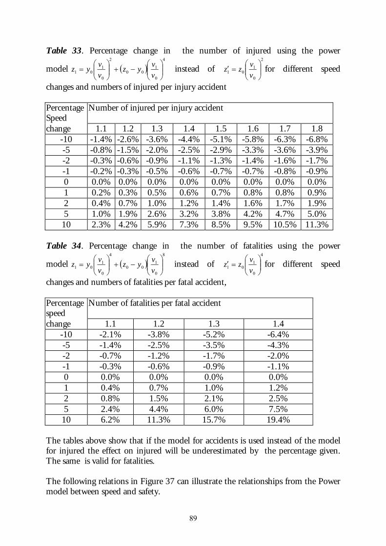
89

Table 33. Percentage change in the number of injured using the power

model ( )4

0

100

2

0

101

−+

=

vvyz

vvyz instead of

2

0

101

=′

vvzz for different speed

changes and numbers of injured per injury accident Percentage Speed

Number of injured per injury accident

change 1.1 1.2 1.3 1.4 1.5 1.6 1.7 1.8 -10 -1.4% -2.6% -3.6% -4.4% -5.1% -5.8% -6.3% -6.8% -5 -0.8% -1.5% -2.0% -2.5% -2.9% -3.3% -3.6% -3.9% -2 -0.3% -0.6% -0.9% -1.1% -1.3% -1.4% -1.6% -1.7% -1 -0.2% -0.3% -0.5% -0.6% -0.7% -0.7% -0.8% -0.9% 0 0.0% 0.0% 0.0% 0.0% 0.0% 0.0% 0.0% 0.0% 1 0.2% 0.3% 0.5% 0.6% 0.7% 0.8% 0.8% 0.9% 2 0.4% 0.7% 1.0% 1.2% 1.4% 1.6% 1.7% 1.9% 5 1.0% 1.9% 2.6% 3.2% 3.8% 4.2% 4.7% 5.0% 10 2.3% 4.2% 5.9% 7.3% 8.5% 9.5% 10.5% 11.3%

Table 34. Percentage change in the number of fatalities using the power

model ( )8

0

100

4

0

101

−+

=

vvyz

vvyz instead of

4

0

101

=′

vvzz for different speed

changes and numbers of fatalities per fatal accident, Percentage speed

Number of fatalities per fatal accident

change 1.1 1.2 1.3 1.4 -10 -2.1% -3.8% -5.2% -6.4% -5 -1.4% -2.5% -3.5% -4.3% -2 -0.7% -1.2% -1.7% -2.0% -1 -0.3% -0.6% -0.9% -1.1% 0 0.0% 0.0% 0.0% 0.0% 1 0.4% 0.7% 1.0% 1.2% 2 0.8% 1.5% 2.1% 2.5% 5 2.4% 4.4% 6.0% 7.5% 10 6.2% 11.3% 15.7% 19.4%

The tables above show that if the model for accidents is used instead of the model for injured the effect on injured will be underestimated by the percentage given. The same is valid for fatalities. The following relations in Figure 37 can illustrate the relationships from the Power model between speed and safety.

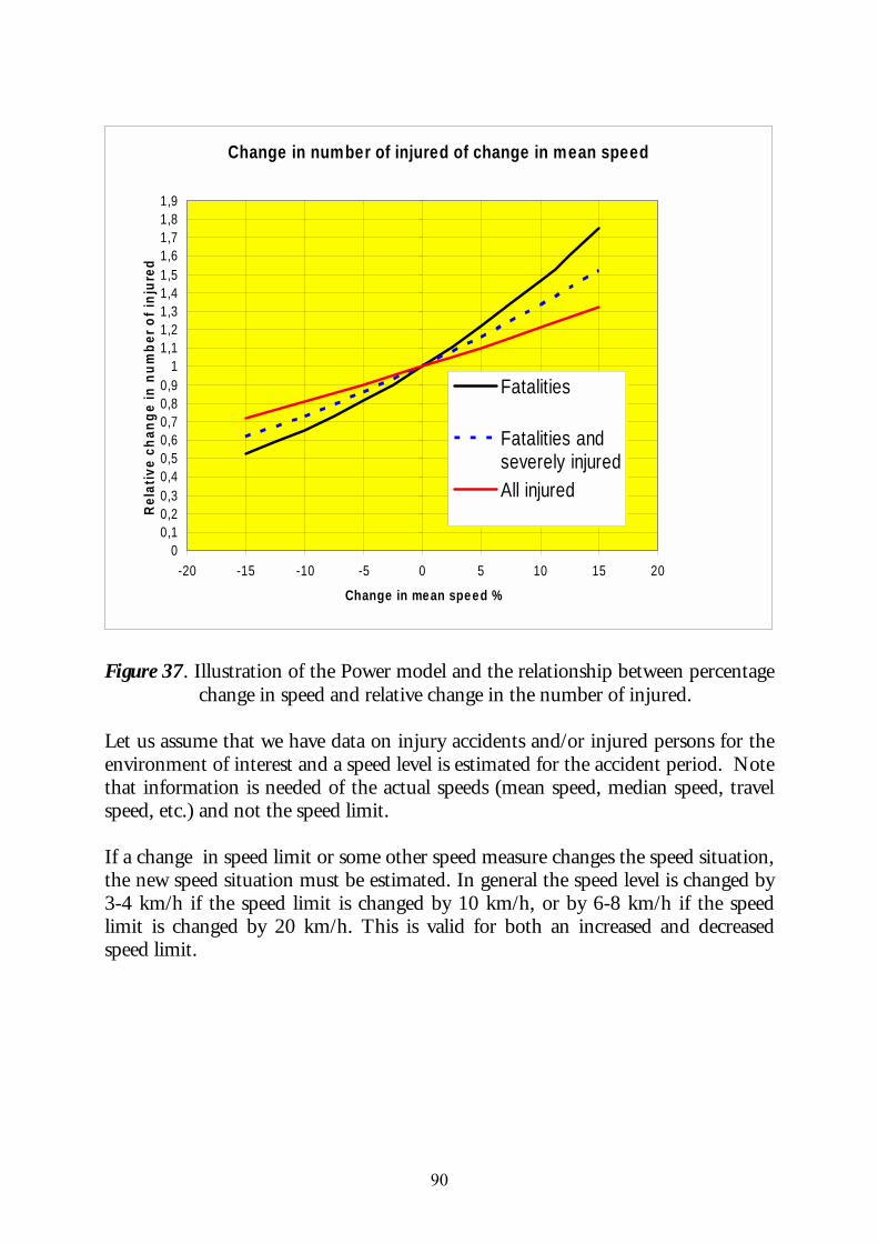
90

Change in number of injured of change in mean speed

00,10,20,30,40,50,60,70,80,9

11,11,21,31,41,51,61,71,81,9

-20 -15 -10 -5 0 5 10 15 20

Change in mean speed %

Rel

ativ

e ch

ange

in n

umbe

r of i

njur

ed

Fatalities

Fatalities andseverely injuredAll injured

Figure 37. Illustration of the Power model and the relationship between percentage

change in speed and relative change in the number of injured. Let us assume that we have data on injury accidents and/or injured persons for the environment of interest and a speed level is estimated for the accident period. Note that information is needed of the actual speeds (mean speed, median speed, travel speed, etc.) and not the speed limit. If a change in speed limit or some other speed measure changes the speed situation, the new speed situation must be estimated. In general the speed level is changed by 3-4 km/h if the speed limit is changed by 10 km/h, or by 6-8 km/h if the speed limit is changed by 20 km/h. This is valid for both an increased and decreased speed limit.

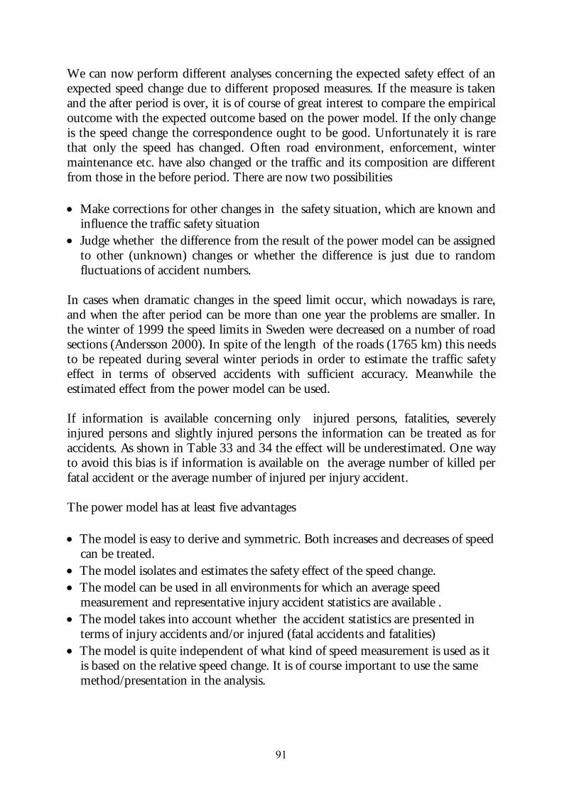
91

We can now perform different analyses concerning the expected safety effect of an expected speed change due to different proposed measures. If the measure is taken and the after period is over, it is of course of great interest to compare the empirical outcome with the expected outcome based on the power model. If the only change is the speed change the correspondence ought to be good. Unfortunately it is rare that only the speed has changed. Often road environment, enforcement, winter maintenance etc. have also changed or the traffic and its composition are different from those in the before period. There are now two possibilities • Make corrections for other changes in the safety situation, which are known and

influence the traffic safety situation • Judge whether the difference from the result of the power model can be assigned

to other (unknown) changes or whether the difference is just due to random fluctuations of accident numbers.

In cases when dramatic changes in the speed limit occur, which nowadays is rare, and when the after period can be more than one year the problems are smaller. In the winter of 1999 the speed limits in Sweden were decreased on a number of road sections (Andersson 2000). In spite of the length of the roads (1765 km) this needs to be repeated during several winter periods in order to estimate the traffic safety effect in terms of observed accidents with sufficient accuracy. Meanwhile the estimated effect from the power model can be used. If information is available concerning only injured persons, fatalities, severely injured persons and slightly injured persons the information can be treated as for accidents. As shown in Table 33 and 34 the effect will be underestimated. One way to avoid this bias is if information is available on the average number of killed per fatal accident or the average number of injured per injury accident. The power model has at least five advantages • The model is easy to derive and symmetric. Both increases and decreases of speed

can be treated. • The model isolates and estimates the safety effect of the speed change. • The model can be used in all environments for which an average speed

measurement and representative injury accident statistics are available . • The model takes into account whether the accident statistics are presented in

terms of injury accidents and/or injured (fatal accidents and fatalities) • The model is quite independent of what kind of speed measurement is used as it

is based on the relative speed change. It is of course important to use the same method/presentation in the analysis.

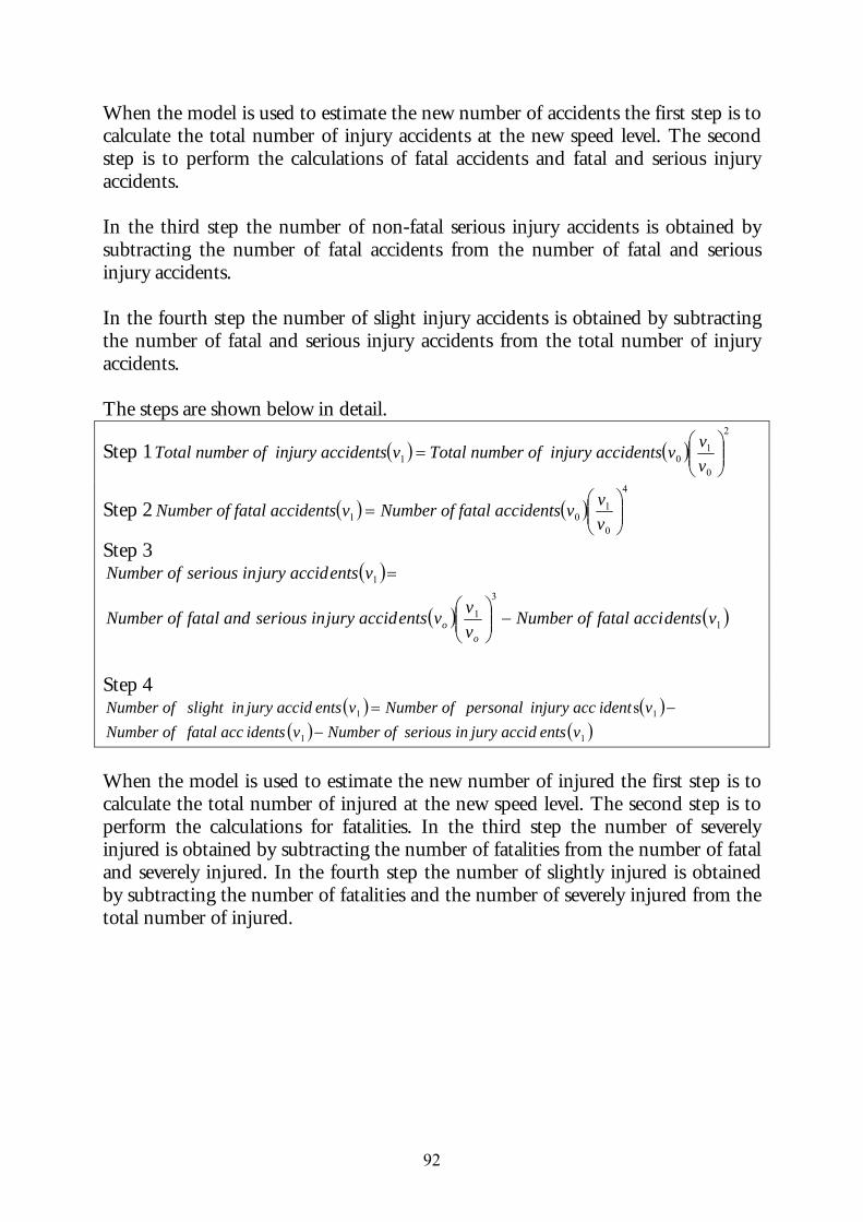
92

When the model is used to estimate the new number of accidents the first step is to calculate the total number of injury accidents at the new speed level. The second step is to perform the calculations of fatal accidents and fatal and serious injury accidents. In the third step the number of non-fatal serious injury accidents is obtained by subtracting the number of fatal accidents from the number of fatal and serious injury accidents. In the fourth step the number of slight injury accidents is obtained by subtracting the number of fatal and serious injury accidents from the total number of injury accidents. The steps are shown below in detail.

Step 1 ( ) ( )2

0

101

=

vvvntsury accideer of injTotal numbvntsury accideer of injTotal numb

Step 2 ( ) ( )4

0

101

=

vvvdentsfatal acciNumber of vdentsfatal acciNumber of

Step 3 ( )

( ) ( )1

3

1

1

vdentsfatal acciNumber of vvventsjury accidserious infatal and Number of

ventsjury accidserious inNumber of

oo −

=

Step 4 ( ) ( )

( ) ( )11

11 s ventsjury accidserious inNumber of vidents fatal accNumber of

videntinjury acc personal Number of ventsjury accidslight inNumber of −

−=

When the model is used to estimate the new number of injured the first step is to calculate the total number of injured at the new speed level. The second step is to perform the calculations for fatalities. In the third step the number of severely injured is obtained by subtracting the number of fatalities from the number of fatal and severely injured. In the fourth step the number of slightly injured is obtained by subtracting the number of fatalities and the number of severely injured from the total number of injured.

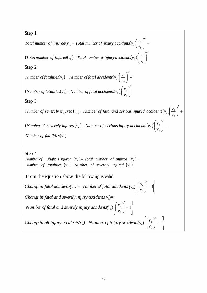
93

Step 1

( ) ( )

( ) ( )( )4

0

100

2

0

101

−

+

=

vvvaccidentsinjuryofnumberTotalvinjuredofnumberTotal

vvvntsury accideer of injTotal numbvureder of injTotal numb

Step 2

( ) ( )

( ) ( )( )8

0

100

4

0

101

−

+

=

vvvdentsfatal acciNumber of vfatalitiesNumber of

vvvdentsfatal acciNumber of vfatalitiesNumber of

Step 3

( ) ( )

( ) ( )( )

( )1

6

0

10

3

0

101

vfatalitiesNumber of vvvaccidentsinjuryseriousofNumbervinjuredseverelyofNumber

vvvaccidentsinjuredseriousfatal and Number of vnjuredseverely iNumber of

o −

−

+

=

Step 4

( ) ( )( ) ( )11

11

vinjuredseverelyofNumbervfatalitiesofNumbervinjuredofnumberTotalvnjured slight iNumber of

−−=

From the equation above the following is valid

Change in fatal accidents(v1) = Number of fatal accidents (v0)

−

1

4

0

1

vv

Change in fatal and severely injury accidents(v1)=

Number of fatal and severely injury accidents(v0)

−

1

3

0

1

vv

Change in all injury accidents(v1)= Number of injury accidents(v0)

−

1

2

0

1

vv

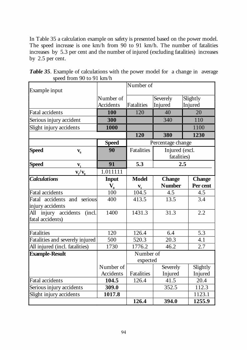
94

In Table 35 a calculation example on safety is presented based on the power model. The speed increase is one km/h from 90 to 91 km/h. The number of fatalities increases by 5.3 per cent and the number of injured (excluding fatalities) increases by 2.5 per cent. Table 35. Example of calculations with the power model for a change in average

speed from 90 to 91 km/h

Example input Number of

Number of Severely Slightly Accidents Fatalities Injured Injured Fatal accidents 100 120 40 20 Serious injury accident 300 340 110 Slight injury accidents 1000 1100 120 380 1230 Speed Percentage change Speed v0 90 Fatalities Injured (excl.

fatalities)

Speed v1 91 5.3 2.5 v1/v0 1.011111 Calculations Input Model Change Change V0 v1 Number Per cent Fatal accidents 100 104.5 4.5 4.5 Fatal accidents and serious injury accidents

400 413.5 13.5 3.4

All injury accidents (incl. fatal accidents)

1400 1431.3 31.3 2.2

Fatalities 120 126.4 6.4 5.3 Fatalities and severely injured 500 520.3 20.3 4.1 All injured (incl. fatalities) 1730 1776.2 46.2 2.7 Example-Result Number of

expected

Number of Severely Slightly Accidents Fatalities Injured Injured Fatal accidents 104.5 126.4 41.5 20.4 Serious injury accidents 309.0 352.5 112.3 Slight injury accidents 1017.8 1123.1 126.4 394.0 1255.9

95

5.8 Conclusions As in all investigations about the safety effect of speed changes, an accurate estimate of the average speed before and after the speed change, together with representative and stable accident statistics, are cornerstones of the model. The origin of the model is based on such investigations. The power model expresses both the risk dimension and the consequence dimension of safety. At the same time it is of course important to identify the changes in traffic safety due to other changes in traffic or control for them in the analysis. The possibilities to improve the power model are in some way limited as the model refers to the kinetic energy (if this assumption is accepted) and the normal accident reporting definitions by the police. As the objective of the model is to isolate the safety effect of the speed change the validation of the model needs information on the effect of other safety measures taken and information on the change or difference in exposure between a before period and an after period. Used as a forecasting model, and there are no other changes than the speed, the last one is not necessary. The model has its main use as a forecasting model and gives an answer to the question: ”What will happen regarding safety if the average speed is changed by x % from the existing speed level and everything else remains unchanged”? Statistical investigations of speed changes in urban areas are rare, due to some extent, to the lack of speed information. The experience, however, shows that the existing results from these few investigations are in good agreement with the power model. In practice the model is based on the injury accident statistics for the environment of interest and the speed level in the environment. This means that if representative accident data and speed data are available the model can be used. Speed variance is also a subject of interest. There is however normally a strong relationship between the speed variance and the average speed. The change in speed variance at a given average speed will not normally change the aggregated kinetic energy in the system. The influence of different accident sources is demonstrated to a certain extent by the accident statistics in different countries. As the corresponding statistical investigations in different countries give the same result the results seem to be independent of different police reporting systems. Fatalities in traffic have normally a high degree of reporting. The composition of injury accident types will however differ between different countries and sources. The results from the power model also make it possible to compare results from other corresponding models. In comparison with other models the power model can be used in a normative way concerning the safety effect of the speed change. As

96

the power model is based on the change in kinetic energy all speed situations can be analysed, at least in theory. The relation of the model to the kinetic energy has also a close relation to forces. The forces in traffic depend not on the speed itself but on the change in speed, the accelerations and the decelerations. Accidents are a subset of the events with (unexpected) decelerations and the higher the speed, the higher are decelerations and the higher is the probability of injuries or fatalities among the involved road users. In investigations of specific accident types these forces on the human body are of great interest in relation to the driving speed level of the motor vehicle. Sometimes there is hesitation in using the model, as it does not make a distinction between different accident types (SNRA 2001). The background of the model is to predict what will happen to the total injury situation concerning fatalities and injured when the kinetic energy in the system changes, which makes it difficult to distinguish an accident type. But if the accidents from an accident type are distributed over fatal accidents, serious injury accidents and slight injury accidents the model can be used even for different accident types, single accidents, head-on collisions, rear-end collisions etc. The model can be regarded as close to reality i.e. valid as the result agrees well with the empirical results concerning injury accident rates. The results indicate, however, that the power model underestimates the effect of speeds on the number of fatalities. Speed is of central importance in the transport sector. Almost all effects of the transport system have a strong relationship with speed or the kinetic energy. Speed is of the highest importance for the outcome of accidents. It is therefore important to include speed in the safety considerations as the probabilities of accidents, injured or fatalities in all transport planning are dependent on speed. The power model is one tool to increase understanding of the importance of average speed changes on an aggregated level concerning both accidents, injured and fatalities.

97

6. Discussion 6.1 Verification of the hypotheses The three-dimensional method to illustrate the traffic safety problem concerning exposure, risk and consequence has been verified among traffic safety experts and seems valuable in describing and analysing the traffic safety problem. When traffic safety problems were presented to the traffic safety experts many of the them gave priority to the fatality rate and injury rate regardless of the number of fatalities. Most of the Swedish and international traffic safety experts, who were asked to give their opinion on a Table or Figure approach, explained that in traffic safety analysis they were more used to tables and less used to figures. An overwhelming majority of these persons preferred the Table to the three-dimensional Figure. The Figure approach indicated a tendency to draw the attention to problems with many fatalities or serious consequences. Most of the experts, however, explained that they want both a Table and a Figure and that a Figure gives a greater understanding of the total traffic safety problem than a Table. The verification of the power model shows that there is a very good correspondence between empirical data and the power model concerning the relation of the number of injury accidents and the number of injured with speed. The effect of speed on the number of fatal accidents and especially on the number of fatalities/fatal accident seems to be underestimated by the model. Even though the model is mainly based on investigations in rural areas, existing investigations in urban areas present similar corresponding results. 6.2 Scientific contribution Traffic safety research shows that multidimensional presentations or approaches are too seldom used in traffic safety work and research. Today, traffic safety work is often only one-dimensional and considers single measures for groups of road users or groups of roads or groups of accidents etc.. Multidimensional approaches enable researchers and traffic safety workers to co-operate to a higher degree but also to realise that one measure will change the safety effect of others. Reducing the speed probably means a higher effect on safety of seatbelt use but a lower effect of alcohol among drivers in traffic. There are some difficulties in considering and evaluating both multidimensional and multidisciplinary approaches. An evaluation of the simultaneous safety effect of several measures and other changes in order to estimate the effect of a single measure must be possible. The multidimensional approach proposed is one tool to use in a simultaneous approach to describe or evaluate the traffic safety effects even if it is limited to the three dimensions of exposure, risk and consequence. This thesis

98

stresses the multidimensional aspects for the people involved in road safety work in making the safety problems more comprehensible. The relation between speed and safety is one of the most investigated relationships in traffic safety. During the last decades speed limits have been changed in most countries and the safety effects of the resulting speed changes have been estimated. All these investigations together show the clear influence of speed changes on safety (Elvik et al 1997). The theory of kinetic energy in the transportation system is used in the power model. The change in kinetic energy is used to explain both the change in injury or fatality risk and the change in consequences, the number of fatalities if injured. Both dimensions show a close relationship to the square of the relative speed changes. The thesis contributes by validating the power model. The main validation data refers to rural areas but investigations of urban areas, winter periods and pedestrian accidents also support the validity of the power model. The only dimension of safety where the power model is not valid is the number of fatalities per fatal accident. Fatalities are even more sensitive to changes in speed than according to the fourth power proposed by the power model. A recent similar study from United Kingdom shows the corresponding results (Taylor M.C. et al 2002). 6.3 Implications for traffic safety work The thesis shows that it is important to take all three basic dimensions of exposure, risk and consequence into account when - performing a diagnosis of the current safety situation and identifying the safety

problem - identifying the most relevant safety measures to tackle those problem - studying the effects of the measures implemented In comparing different traffic safety problems it is important to consider if the traffic safety problem is an exposure problem, a risk problem or a consequence problem. The three-dimensional presentation gives a very quick illustration of this as demonstrated in the thesis. Once it has been decided if it is an exposure, risk or consequence problem, it is easier to identify the relevant safety measures. In case of an exposure problem the effect of the measure shall be to reduce the exposure in order to decrease the traffic safety problem. In the case of a risk problem, the measures which reduce the risk

99

shall be used. If it is a consequence problem, the measures which reduce the consequence are of interest. Measures ought to be classified according to their main effect. Speed measures influence both risk and consequence. The same is for example also valid for motorways in the road network compared with two-lane roads. In evaluating the safety effect of measures or describing the total traffic safety situation it is of great value to realise how the exposure has developed. Otherwise it is not possible to evaluate how the measures have influenced the risk. The consequence evaluation need a stable source of the reporting of traffic accidents or injured persons. The power model is unique in the sense that it express the isolated expected effect of the speed change on safety. The model can be used to - estimate the expected effect of speed changes - study the safety effect of speed measures - isolate the speed effect on safety from other effects - isolate the possible speed effects of a specific measure taken or the influence of

speed changes at the same time as the safety effect of the measure is evaluated. The model has many advantages as it is general, flexible and easy to memorize, and can use both accident and injury data. Often it is of great interest in traffic safety programmes to give information on how the existing speed situation will change in the future. The power model can be used to forecast how the safety situation will be changed independent of other expected changes. The model can be used in before and after studies of the traffic safety situation to estimate the isolated traffic safety effect of the speed change between the two periods. The model can also be used in order to compare the safety results of different speed measures and to reveal if some other unexpected or suspected changes affecting safety have occurred. The opposite is also possible if a measure shows an unexpected speed change. Then the effect of the speed change can be estimated by the model and isolated from or compared to the estimated total effect of the measure. This is probably the case concerning many traffic safety measures. Speed measurements are, however, often not available or not used in the analysis.

100

The above put high demands on speed measurements and representative accident statistics in addition to the need of exposure data expressed earlier. It is of utmost importance to include an investigation of the changes in speed in all studies on the effect of safety measures. 6.4 Future research needs Traffic safety is a multidimensional and multidisciplinary problem. The need for future research can be expressed by three wishes. The first wish is a practical one; that general computer software will be developed to create three-dimensional presentations. This is a step to open up a visualization of the different dimensions of a traffic safety problem in traffic safety research. The second wish is that the future research should make it possible to estimate multidimensional effects of changes of traffic safety measures in traffic. This is important in order to both introduce and to evaluate a traffic safety measure. When a lot of measures are presented in a national traffic safety programme this knowledge is important. It is especially important to know how the measures influence each other´s effects. The last is of great interest in e.g. research concerning the effects on exposure of different traffic safety measures, which seldom are analysed. The interest in exposure will probably increase among researchers as the interest to regulate the traffic is increasing, especially in large urban areas. As the use of speed measures increases rapidly in urban areas the interest in their traffic safety effect and in their effect on exposure calls for a multidimensional research approach to find sustainable solutions. For example how will speed changes or motorway solutions influence the exposure? This is a field for research as the knowledge about the effects on exposure is limited today. The third wish concerns speed research. When the speed situation changes in urban areas further validations of the power model are possible if both speed and accident information are available. That can also make it possible to investigate the effect of car speed on the safety of different road user groups at the same time as normally a lot of other traffic safety measures are introduced. This is of course also valid for different accident types in different environments. As the accident situation in areas with low car speeds is quite safe for car occupants and there are few injured car occupants but numerous property damage accidents, the power model and corresponding models ought to include these accidents. The alternative to just looking at injured car occupants will otherwise result in very long-term research projects. The projects probably need an investigation period of 5-10 years.

101

In addition to the above three wishes it will of course also be urgent to consider the speed and exposure situation at the same time for different groups in traffic, vehicle groups, driver groups, etc. in different conditions and on different types of roads. This is made possible by the development of new “on line” registration methods concerning the speed and the use (exposure) of the cars. This opens up new possibilities for pursuing traffic safety as well as other transport policy objectives.

102

References Ashton, S.J. Pedder, J.B. Mackay, G.M. (1977) Pedestrian injuries and car Exterior. SAE Transactions, New York. Paper 770092, 1977. Allsop, R (1995). Traffic injuries resulting from excess and inappropriate speed. European Transport Safety Council, 1995. Andersson, G. (2000) Reduced speed limits during the winter 1999/2000. Effects on safety, speed and acceptance. VTI Notat 58-2000. Asmussen, E & Krankenburg, A.(1982). An analysis of the traffic phenomenon. Publication 1982-1E. SWOV 1982. Brüde, U & Wretling, P (1998). 13-m vägar � samband utformning, hastigheter och olyckor PM revised 1998-01-21 Carlsson, G (2002) Vad bestämmer dödsrisken och hur beror antalet dödade personer i en given väg- och trafikmiljö av medelhastigheten. Transportforum 2002. VTI Konferens 21, 2002. COST 329 (1998). Models for traffic and safety development and interventions. European Commision 1998. Ekman, L (1996). On the treatment of flow in traffic safety analysis: A non-parametric approach applied on vulnerable road users. Lunds Universitet. Trafikteknik. Bulletin 136, 1996. Elvik, R, Vaa, T, Østvik, E. Trafikksikkerhetshåndbok, (1990) Transportokonomisk institutt, Oslo 1990. Page 184-186 (In Norwegian).

Elvik, R, Vaa, T, Mysen, A,B. Trafikksikkerhetshåndbok, (1997) Transportokonomisk institutt, Oslo 1997. Page 313-316 (In Norwegian). Elvik, R & Amundsen A.H. (2000) Improving Road Safety in Sweden. Institute of Transport Economics, Oslo, Report 490/2000 Engel, U & Thomsson, L K. (1988) Speeds, speed limits and accidents. RfT, Report 3 1988. (In Danish. Summery in English) Evans, L. (1991) Traffic Safety and the Driver. ISBN 0-422-00163-0, 1991. Page 153-154 and 322. Evans, L .(2001) Age and fatality risk from similar severity impacts. Journal of Traffic Medicine, Volume 29, No 1-2, 2001.

103

ETSC. (1999) Exposure data for travel risk assessment. Current practice and future needs. ETSC. 1999. Frith, B. (2000) Road Safety Management in New Zeeland. International seminar on road traffic and accident data needs for the new century. OECD/IRTAD, Vienna, September 2000. Gaudry, M & Lassarre, S (2000) Structural road accident models. The international DRAG family. Pergamon press 2000. Haddon, W. Jr. (1972) A logical framework for categorizing highway safety phenomena and activity. Journal of trauma, 12:193-207, 1972. Hauer, E (2000) Prediction of the Expected Safety Performance of Rural Two-lane Highways. US Department of Transportation. Federal Highway Administration, Publication No, FHWA-RD-99-207, 2000. Holmberg, B. & Hydén, C. et al. (1996) Trafiken i samhället. Grunder för planering och utformning. Studentlitteratur 1996. IRTAD (2000), International Road Traffic Accident Database, OECD/BaSt, (www.irtad.de). Kallberg, V-P (1998) The two effects of speed on accidents: Number and severity. Transportation Research Board, Paper No. 981191, January 11-15, 1998. Krafft, M. Non-fatal injuries to car occupants. Karolinska Institutet/Folksam 1998. Ljungblad, L (2000). Road barriers and traffic safety. VTI rapport 453, 2000. Nilsson, G. (1977) Trials with speed limits during the years 1968-1972. VTI Report 117A, 1977. Nilsson, G. (1978) Risk exposures. A structure of needs of risk exposures. VTI Report 144, 1978 (Summary in English). Nilsson, G. (1980) Change of maximum speed limit from 110 to 90 km/h during the summer period 1979 in Sweden. VTI Meddelande 197, 1980 (Summary in English) Nilsson, G. (1981a) The effects of speed limits on traffic accidents in Sweden. International Symposium.OECD Dublin 1981. Nilsson, G. (1981b) Traffic safety in terms of accidents, injuries, risks and consequences- a multidimensional method for description of traffic safety situation. Road Design and Safety. IX:th IRF World Meeting Stockholm 1981. Nilsson, G. (1984a) A review of the traffic safety situation in Sweden with regard to different strategies and methods of evaluating traffic safety measures VTI Reprint 121. (reprint from Journal of Occupational Accidents, 6(1984) 35-47). Nilsson, G. (1984b) Speeds, accident rates and personal injury consequence for different road types. VTI Report 277, 1984 (Summary in English).

104

Nilsson, G. (1990) Reduction in the speed limit from 110 km/h to 90 km/h during summer 1989. Effects on personal injury accidents, injures and speeds. VTI Report 358 A, 1990. OECD. (1997a) Road safety principles and models. OECD, Road Transport Research, 1997. OECD. (1997b) Road safety principles and models: Review of descriptive, predictive, risk and accident consequence models, Road Transport Research, OECD/GD(97)153, 1997. Pasanen, E. (1992) Driving speeds and pedestrian safety; A mathematical model. Helsinki University o Technology Transport Engineering, Publication 76, Otaniemi 1992. Peltola, H. (2000) Effect of seasonal changing speed limits on speeds and accidents. Transportation Research Board, Paper No. 001482, January 9-13, 2000´. Road traffic injuries 1997,1998 and 1999. Official Statistics of Sweden, Statistics Sweden.

Roosmark, P-O. & Fräki, R. (1970) Interview investigation of road traffic accidents. VTI Rapport 106, 1970. SNRA (2001) Den eviga hastighetsfrågan - och dess följdfrågor. Swedish National Road Administration. Publikation 2001:24. Spolander, K. (1999) Staden, bilen, farten. NTF:s förlag och service AB, 1999. Statistics Sweden. (1999) National travel survey, NTS, 1999. Official Statistics of Sweden, Statistics Sweden. Statistics Sweden.(2000) Road Traffic Injuries 1997, 1998, 1999. Official Statistics of Sweden, Statistics Sweden. 2000. Taylor M.C. et al (2002) The relationship between speed and accidents on rural single-carriageway roads. TRL Report TRL511, 2002. Thulin, H. (1987) Traffic accidents and injured reported by police, hospitals and insurance in the county of Östergötland 1983-1984. VTI Meddelande 547, 1987 (In Swedish) Thulin, H. & Nilsson, G. (1994) Road traffic, exposure, injury risks and injury consequences for different travel modes and age groups. VTI Report 390 A, 1994. Wass, C. (1977) Traffic Accident Exposure and Liability. Allerod 1977. Webster,D.C. & Mackie, A.M. (1996) Review of traffic calming schemes in 20 mph zones. TRL Report 215, 1996

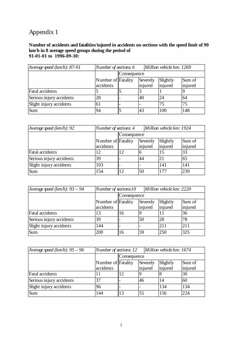
i

Appendix 1 Number of accidents and fatalities/injured in accidents on sections with the speed limit of 90 km/h in 8 average speed groups during the period of 91-01-01 to 1996-09-30: Average speed (km/h): 87-91 Number of sections: 6 Million vehicle km: 1269 Consequence Number of

accidents Fatality Severely

injured Slightly injured

Sum of injured

Fatal accidents 5 5 3 1 9 Serious injury accidents 28 - 40 24 64 Slight injury accidents 61 - - 75 75 Sum 94 5 43 100 148 Average speed (km/h): 92 Number of sections: 4 Million vehicle km: 1924 Consequence Number of

accidents Fatality Severely

injured Slightly injured

Sum of injured

Fatal accidents 12 12 6 15 33 Serious injury accidents 39 - 44 21 65 Slight injury accidents 103 - - 141 141 Sum 154 12 50 177 239 Average speed (km/h): 93 – 94 Number of sections:10 Million vehicle km: 2220 Consequence Number of

accidents Fatality Severely

injured Slightly injured

Sum of injured

Fatal accidents 13 16 9 11 36 Serious injury accidents 39 - 50 28 78 Slight injury accidents 144 - - 211 211 Sum 200 16 59 250 325 Average speed (km/h): 95 – 96 Number of sections: 12 Million vehicle km: 1674 Consequence Number of

accidents Fatality Severely

injured Slightly injured

Sum of injured

Fatal accidents 11 12 9 8 30 Serious injury accidents 37 - 46 14 60 Slight injury accidents 96 - - 134 134 Sum 144 13 55 156 224

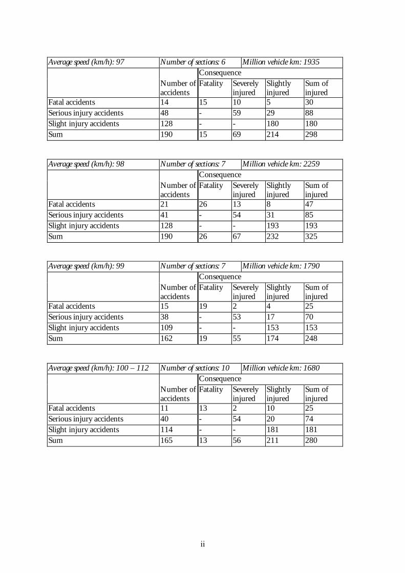
ii

Average speed (km/h): 97 Number of sections: 6 Million vehicle km: 1935 Consequence Number of

accidents Fatality Severely

injured Slightly injured

Sum of injured

Fatal accidents 14 15 10 5 30 Serious injury accidents 48 - 59 29 88 Slight injury accidents 128 - - 180 180 Sum 190 15 69 214 298 Average speed (km/h): 98 Number of sections: 7 Million vehicle km: 2259 Consequence Number of

accidents Fatality Severely

injured Slightly injured

Sum of injured

Fatal accidents 21 26 13 8 47 Serious injury accidents 41 - 54 31 85 Slight injury accidents 128 - - 193 193 Sum 190 26 67 232 325 Average speed (km/h): 99 Number of sections: 7 Million vehicle km: 1790 Consequence Number of

accidents Fatality Severely

injured Slightly injured

Sum of injured

Fatal accidents 15 19 2 4 25 Serious injury accidents 38 - 53 17 70 Slight injury accidents 109 - - 153 153 Sum 162 19 55 174 248 Average speed (km/h): 100 – 112 Number of sections: 10 Million vehicle km: 1680 Consequence Number of

accidents Fatality Severely

injured Slightly injured

Sum of injured

Fatal accidents 11 13 2 10 25 Serious injury accidents 40 - 54 20 74 Slight injury accidents 114 - - 181 181 Sum 165 13 56 211 280

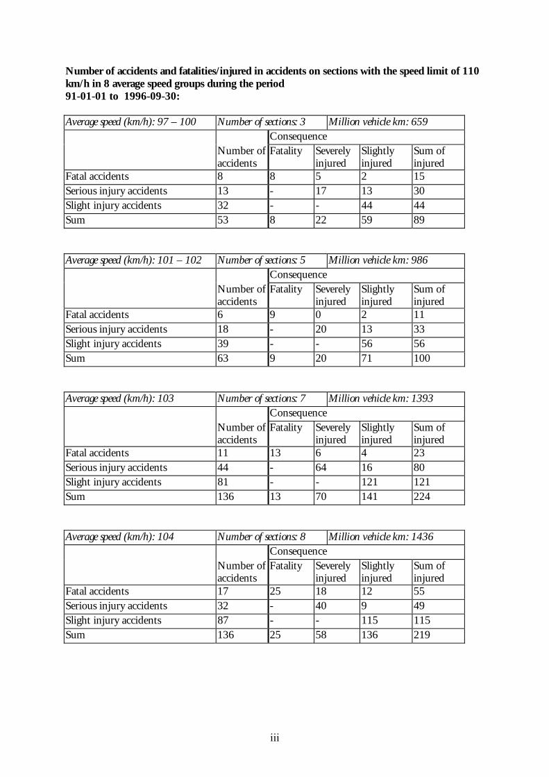
iii

Number of accidents and fatalities/injured in accidents on sections with the speed limit of 110 km/h in 8 average speed groups during the period 91-01-01 to 1996-09-30: Average speed (km/h): 97 – 100 Number of sections: 3 Million vehicle km: 659 Consequence Number of

accidents Fatality Severely

injured Slightly injured

Sum of injured

Fatal accidents 8 8 5 2 15 Serious injury accidents 13 - 17 13 30 Slight injury accidents 32 - - 44 44 Sum 53 8 22 59 89 Average speed (km/h): 101 – 102 Number of sections: 5 Million vehicle km: 986 Consequence Number of

accidents Fatality Severely

injured Slightly injured

Sum of injured

Fatal accidents 6 9 0 2 11 Serious injury accidents 18 - 20 13 33 Slight injury accidents 39 - - 56 56 Sum 63 9 20 71 100 Average speed (km/h): 103 Number of sections: 7 Million vehicle km: 1393 Consequence Number of

accidents Fatality Severely

injured Slightly injured

Sum of injured

Fatal accidents 11 13 6 4 23 Serious injury accidents 44 - 64 16 80 Slight injury accidents 81 - - 121 121 Sum 136 13 70 141 224 Average speed (km/h): 104 Number of sections: 8 Million vehicle km: 1436 Consequence Number of

accidents Fatality Severely

injured Slightly injured

Sum of injured

Fatal accidents 17 25 18 12 55 Serious injury accidents 32 - 40 9 49 Slight injury accidents 87 - - 115 115 Sum 136 25 58 136 219

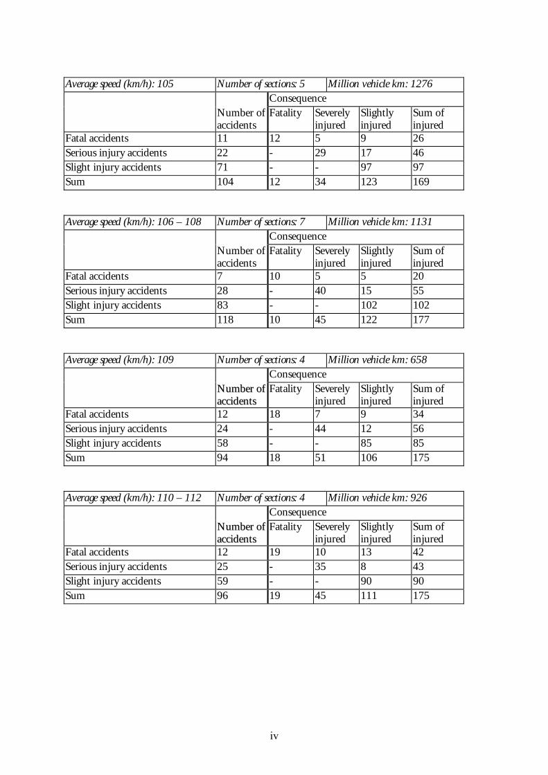
iv

Average speed (km/h): 105 Number of sections: 5 Million vehicle km: 1276 Consequence Number of

accidents Fatality Severely

injured Slightly injured

Sum of injured

Fatal accidents 11 12 5 9 26 Serious injury accidents 22 - 29 17 46 Slight injury accidents 71 - - 97 97 Sum 104 12 34 123 169 Average speed (km/h): 106 – 108 Number of sections: 7 Million vehicle km: 1131 Consequence Number of

accidents Fatality Severely

injured Slightly injured

Sum of injured

Fatal accidents 7 10 5 5 20 Serious injury accidents 28 - 40 15 55 Slight injury accidents 83 - - 102 102 Sum 118 10 45 122 177 Average speed (km/h): 109 Number of sections: 4 Million vehicle km: 658 Consequence NNuummbbeerr ooff

aacccciiddeennttss Fatality Severely

injured Slightly injured

Sum of injured

Fatal accidents 12 18 7 9 34 Serious injury accidents 24 - 44 12 56 Slight injury accidents 58 - - 85 85 Sum 94 18 51 106 175 Average speed (km/h): 110 – 112 Number of sections: 4 Million vehicle km: 926 Consequence NNuummbbeerr ooff

aacccciiddeennttss Fatality Severely

injured Slightly injured

Sum of injured

Fatal accidents 12 19 10 13 42 Serious injury accidents 25 - 35 8 43 Slight injury accidents 59 - - 90 90 Sum 96 19 45 111 175

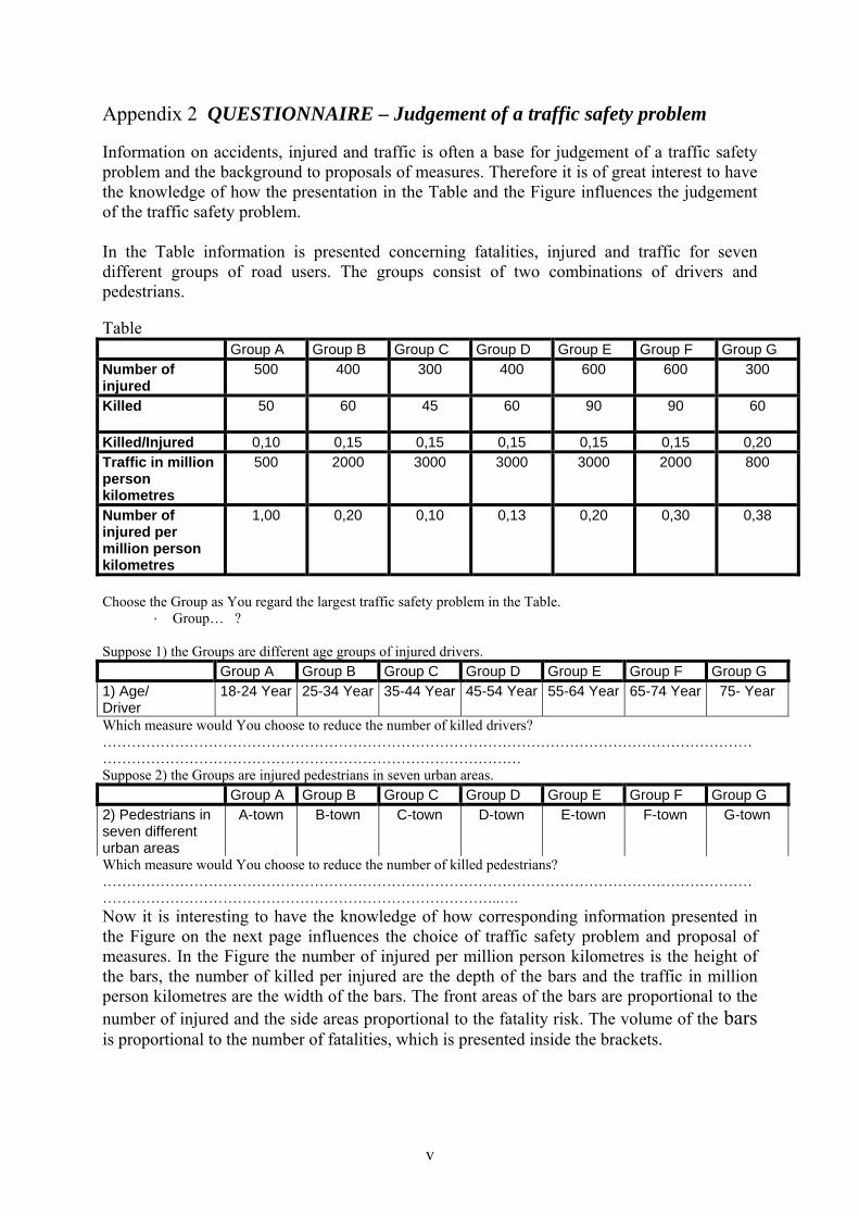
v

Appendix 2 QUESTIONNAIRE – Judgement of a traffic safety problem Information on accidents, injured and traffic is often a base for judgement of a traffic safety problem and the background to proposals of measures. Therefore it is of great interest to have the knowledge of how the presentation in the Table and the Figure influences the judgement of the traffic safety problem. In the Table information is presented concerning fatalities, injured and traffic for seven different groups of road users. The groups consist of two combinations of drivers and pedestrians. Table Group A Group B Group C Group D Group E Group F Group G Number of injured

500 400 300 400 600 600 300

Killed

50 60 45 60 90 90 60

Killed/Injured 0,10 0,15 0,15 0,15 0,15 0,15 0,20 Traffic in million person kilometres

500 2000 3000 3000 3000 2000 800

Number of injured per million person kilometres

1,00 0,20 0,10 0,13 0,20 0,30 0,38

Choose the Group as You regard the largest traffic safety problem in the Table. · Group� ? Suppose 1) the Groups are different age groups of injured drivers. Group A Group B Group C Group D Group E Group F Group G 1) Age/ Driver

18-24 Year 25-34 Year 35-44 Year 45-54 Year 55-64 Year 65-74 Year 75- Year

Which measure would You choose to reduce the number of killed drivers? �������������������������������������������������������������������������� Suppose 2) the Groups are injured pedestrians in seven urban areas. Group A Group B Group C Group D Group E Group F Group G 2) Pedestrians in seven different urban areas

A-town B-town C-town D-town E-town F-town G-town

Which measure would You choose to reduce the number of killed pedestrians? ������������������������������������������������������������������������..�. Now it is interesting to have the knowledge of how corresponding information presented in the Figure on the next page influences the choice of traffic safety problem and proposal of measures. In the Figure the number of injured per million person kilometres is the height of the bars, the number of killed per injured are the depth of the bars and the traffic in million person kilometres are the width of the bars. The front areas of the bars are proportional to the number of injured and the side areas proportional to the fatality risk. The volume of the bars is proportional to the number of fatalities, which is presented inside the brackets.

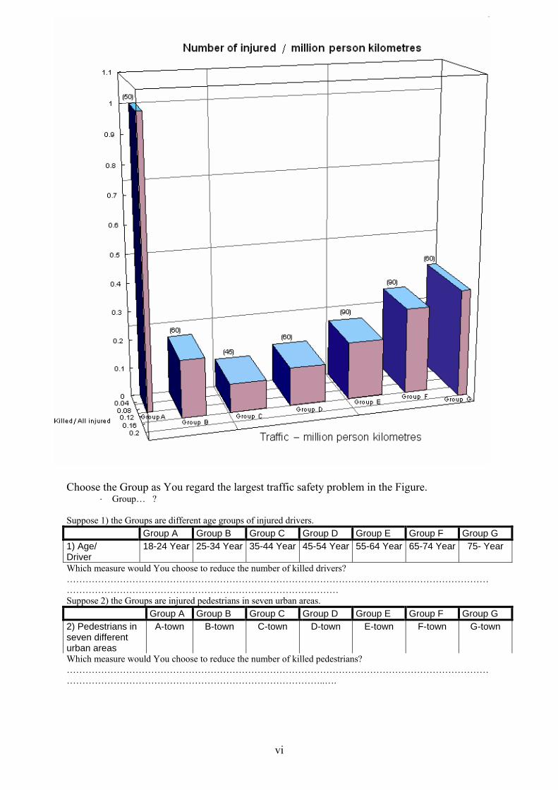
vi

Choose the Group as You regard the largest traffic safety problem in the Figure. · Group� ? Suppose 1) the Groups are different age groups of injured drivers. Group A Group B Group C Group D Group E Group F Group G 1) Age/ Driver

18-24 Year 25-34 Year 35-44 Year 45-54 Year 55-64 Year 65-74 Year 75- Year

Which measure would You choose to reduce the number of killed drivers? �������������������������������������������������������������������������� Suppose 2) the Groups are injured pedestrians in seven urban areas. Group A Group B Group C Group D Group E Group F Group G 2) Pedestrians in seven different urban areas

A-town B-town C-town D-town E-town F-town G-town

Which measure would You choose to reduce the number of killed pedestrians? ������������������������������������������������������������������������..�.

(xx)=Antalet dödade

(xx) = Antalet dödade

vii

Now You have seen the traffic safety problem presented by a three-dimensional Figure and presented by a Table. What is Your opinion? Here are some final questions. If I have to make the choice I will prefer (Yes or No) The Table���� The Figure����. Both the Figure and the Table������ Which advantage has the Table? ������������������������������. ������������������������������. ������������������������������.. Which advantage has the Figure? ������������������������������. ������������������������������. ������������������������������.. Which disadvantage has the Table? ������������������������������. ������������������������������. ������������������������������.. Which disadvantage has the Figure? ������������������������������. ������������������������������. ������������������������������.. When You have answered the questions can You, please, return the answers to goran.nilsson@vti.se . Thanks.