Traffic Flow Anil Kantak

Transportation and

Traffic Flow

Anil V. Kantak

1

Traffic Flow Anil Kantak

•Vehicular Flow:

•When fixed facilities are used simultaneously by streams of vehicles, a vehicular flow is constructed.

•Resulting traffic conditions may be almost free flow when only a few unconstrained vehicles are present on the roadway.

•Resulting traffic condition may be a highly congested flow condition when a lot of streams are combined together.

•Traffic rules and regulations try to maximize their speeds while maintaining an acceptable level of safety. This is usually achieved by

2

Traffic Flow Anil Kantak

Adjusting the distance between vehicles by adjusting the vehicular speed.

• Basic Variables of Traffic Flow:

• Flow

• Concentration

• Mean Speed

Fundamental relationship between these variables is postulated and applied to several traffic flow conditions.

•Vehicular Following:

Distance between subsequent vehicles is computed that is safe if the leading vehicle needs to decelerate suddenly.

3

Traffic FlowAnil Kantak

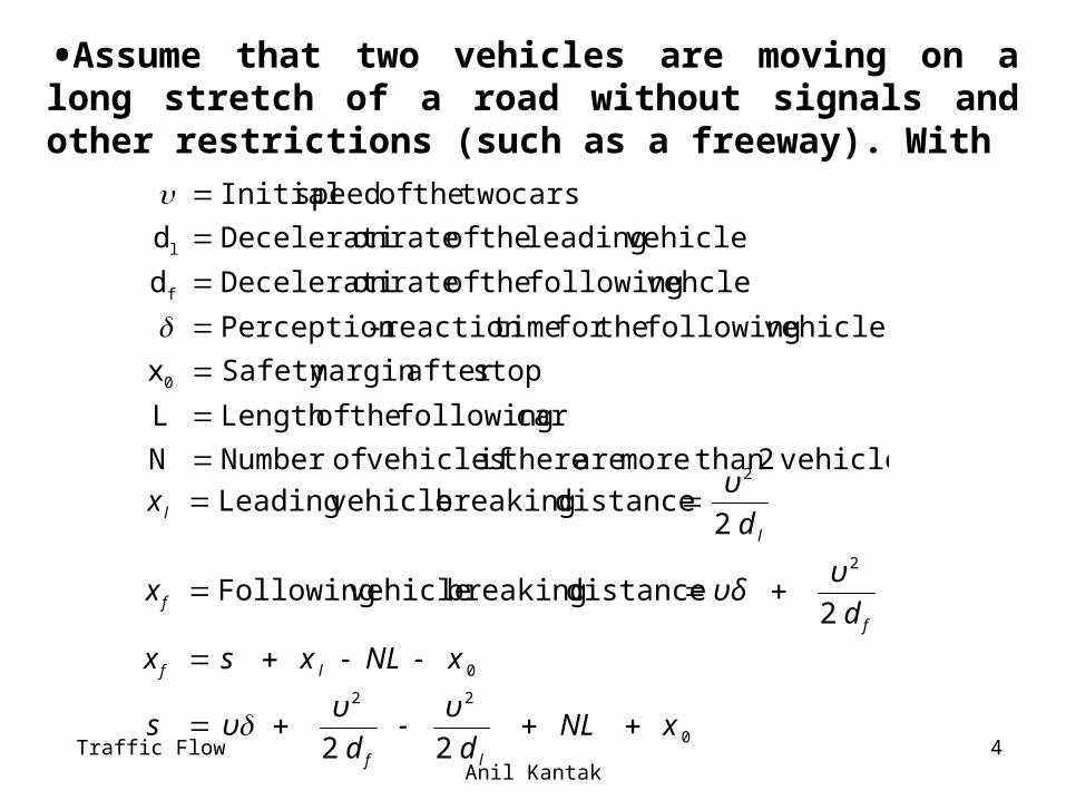
•Assume that two vehicles are moving on a long stretch of a road without signals and other restrictions (such as a freeway). With

vehicles 2 than more are there if vehicles of Number N

car following the of Length L

stop after marginSafety x

vehicle following the for time reaction-Perception

vehcle following the of rate onDecelerati d

vehicle leading the of rate onDecelerati d

cars two the of speed Initial

0

f

l

0

22

0

2

2

22

2

distance breaking vehicle Following

2 distance breaking vehicle Leading

x NL d

υ -

d

υ υs

x - NL - x s x

d

υ υδ x

d

υx

lf

lf

f

f

l

l

4

Traffic Flow Anil Kantak

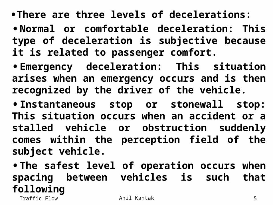
•There are three levels of decelerations:

•Normal or comfortable deceleration: This type of deceleration is subjective because it is related to passenger comfort.

•Emergency deceleration: This situation arises when an emergency occurs and is then recognized by the driver of the vehicle.

•Instantaneous stop or stonewall stop: This situation occurs when an accident or a stalled vehicle or obstruction suddenly comes within the perception field of the subject vehicle.

•The safest level of operation occurs when spacing between vehicles is such that following

5

Traffic Flow Anil Kantak

vehicle can safely stop by applying normal deceleration even when leading vehicle comes to a stonewall stop.

• In general, the higher the level of safety, higher is required spacing just to avoid a collision. However, by increasing the level of safety, capacity of system, i.e., the maximum number of vehicles or passengers that can be accommodated during a given period of time suffers. Consequently, a trade-off between safety and capacity must be done.

•Spacing and Concentration: Suppose cars are uniformly spaced on a length of roadway and they are all going with a uniform speed. 6

Traffic Flow Anil Kantak

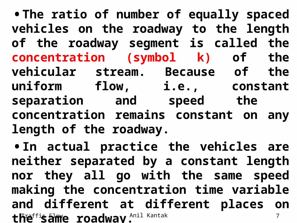
•The ratio of number of equally spaced vehicles on the roadway to the length of the roadway segment is called the concentration (symbol k) of the vehicular stream. Because of the uniform flow, i.e., constant separation and speed the concentration remains constant on any length of the roadway.

•In actual practice the vehicles are neither separated by a constant length nor they all go with the same speed making the concentration time variable and different at different places on the same roadway.

7

Traffic Flow Anil Kantak

Density k

l sionConcentrat

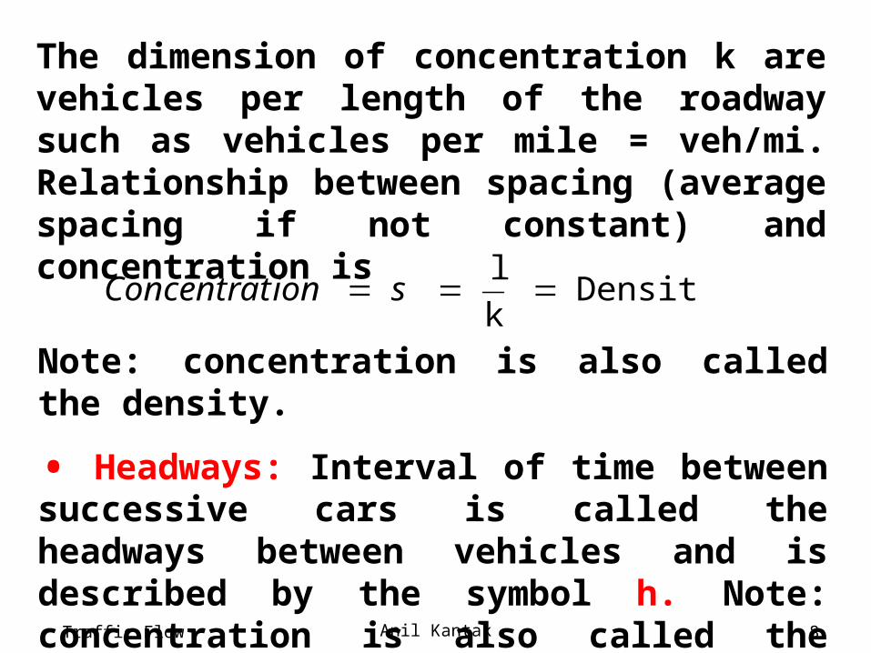
The dimension of concentration k are vehicles per length of the roadway such as vehicles per mile = veh/mi. Relationship between spacing (average spacing if not constant) and concentration is

Note: concentration is also called the density.

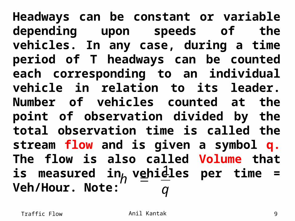
• Headways: Interval of time between successive cars is called the headways between vehicles and is described by the symbol h. Note: concentration is also called the density of the flow.

8

Traffic Flow Anil Kantak

Headways can be constant or variable depending upon speeds of the vehicles. In any case, during a time period of T headways can be counted each corresponding to an individual vehicle in relation to its leader. Number of vehicles counted at the point of observation divided by the total observation time is called the stream flow and is given a symbol q. The flow is also called Volume that is measured in vehicles per time = Veh/Hour. Note:

q h

1

9

Traffic Flow Anil Kantak

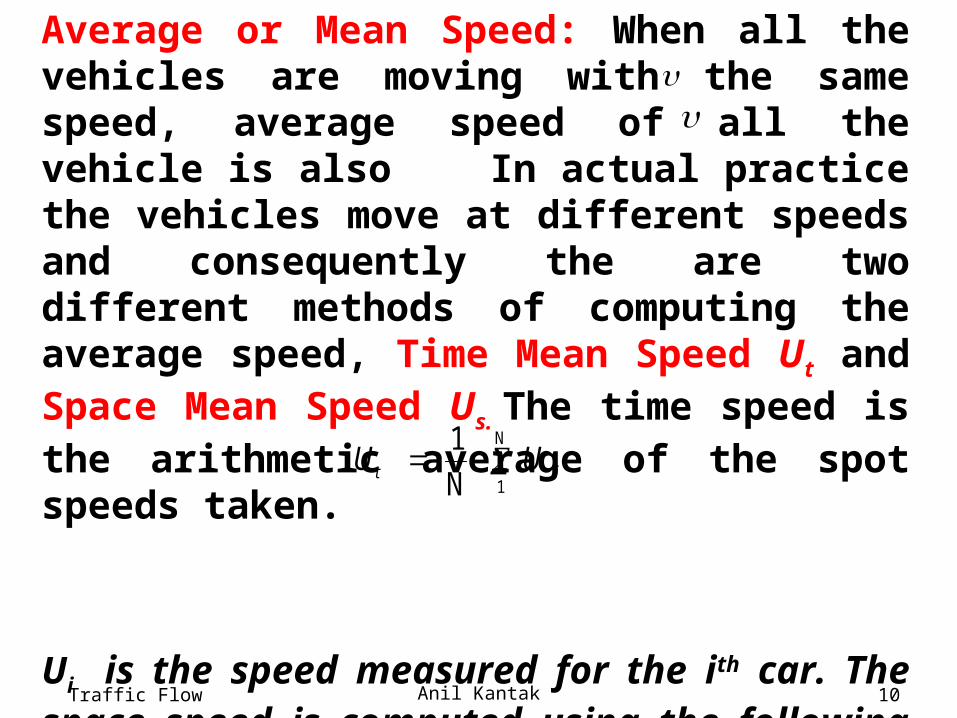
Average or Mean Speed: When all the vehicles are moving with the same speed, average speed of all the vehicle is also In actual practice the vehicles move at different speeds and consequently the are two different methods of computing the average speed, Time Mean Speed Ut and Space Mean Speed Us. The time speed is the arithmetic average of the spot speeds taken.

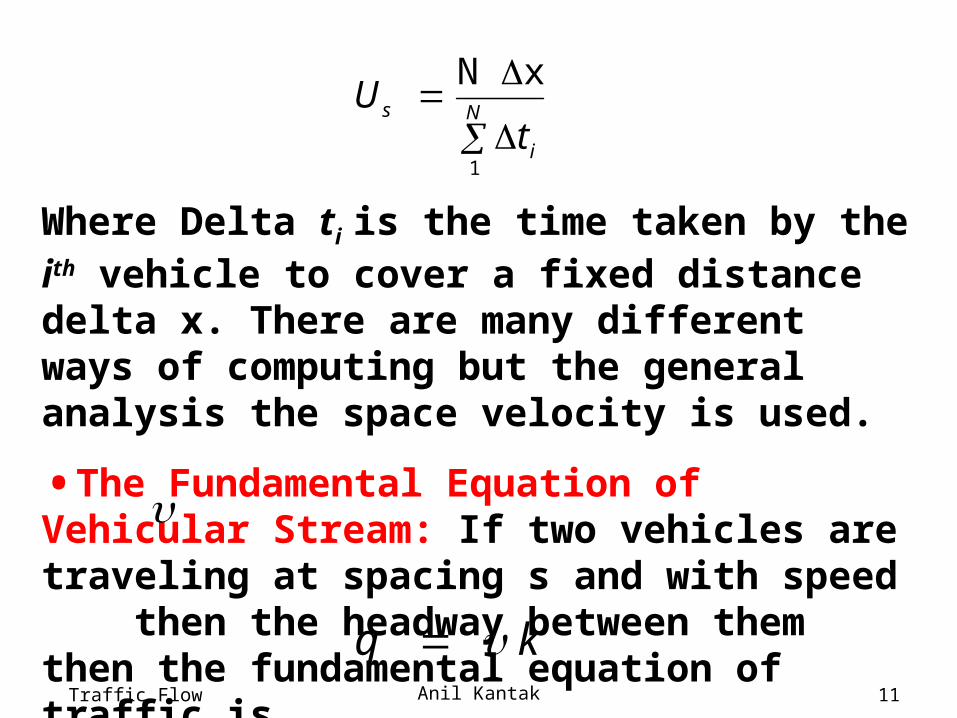
Ui is the speed measured for the ith car. The space speed is computed using the following equation

N

1

N

1 it UU

10

Anil Kantak

N

i

s

tU

1

x N

Where Delta ti is the time taken by the ith vehicle to cover a fixed distance delta x. There are many different ways of computing but the general analysis the space velocity is used.

•The Fundamental Equation of Vehicular Stream: If two vehicles are traveling at spacing s and with speed then the headway between them then the fundamental equation of traffic is

k q Traffic Flow 11

Anil Kantak

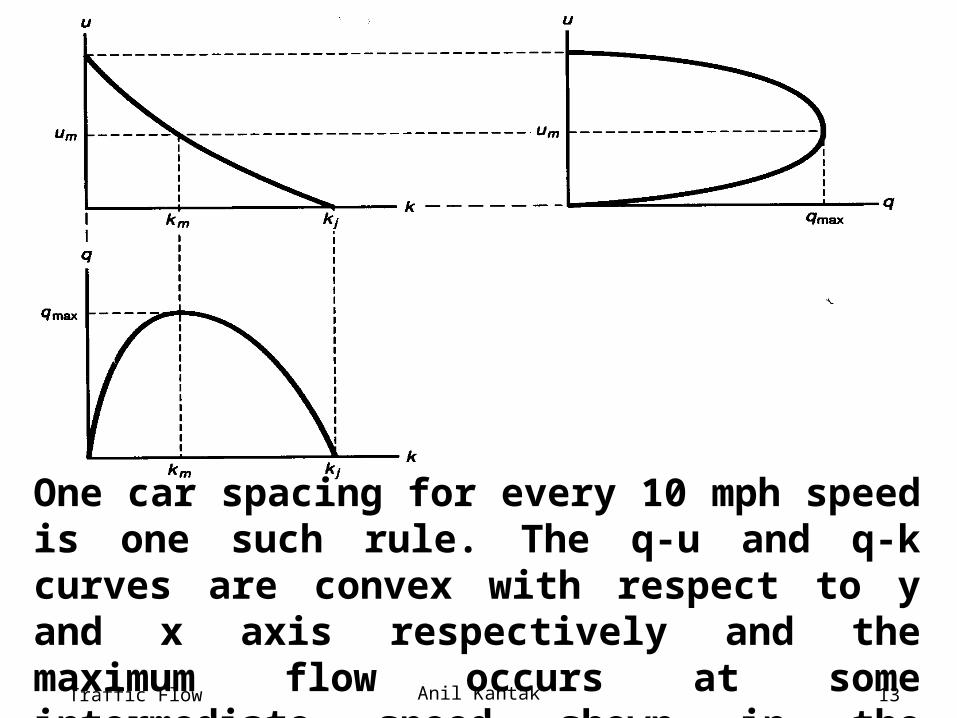
•Highway Traffic flow: In case of highway (freeway) traffic the drivers make their own decisions regarding speed and headway tradeoff. Some drivers keep close to leading car and keep their speed high and safety low while others keep long distances between cars keeping the speed low but safety high. In addition, the freeway vehicles are not all the same. All these differences results in a statistical clustering of vehicles on the roadways. Next slide demonstrates the u-k, u-k, and q-k diagrams for traffic flow on freeways (highways). u-k relationship is monotonically decreasing that is depiction of the rule the drivers follow one another on the average.

Traffic Flow 12

Anil Kantak

One car spacing for every 10 mph speed is one such rule. The q-u and q-k curves are convex with respect to y and x axis respectively and the maximum flow occurs at some intermediate speed shown in the diagrams. Traffic Flow 13

•Stream Measurements The method of least squares can be used to determine the relationship between two or more variables based on a set of experimental observations. Many vehicular stream measurements are available in practice. Because flow, speed and concentration are interrelated, any measurement method used must measure two of the variables simultaneously the third may be estimated by the equation given above. It should be noted that measuring only one variable does not serve the purpose.

•The moving observer method. This method is developed to provide simultaneous measurements while moving in relation to the

traffic stream being measured. To understand this better, consider the following two cases first.

Case I: Observer is stationary and the traffic stream is moving, If N0 vehicles overtake the observer during the period of observation, T then the observed flow q is given by

T q N T

N q 0

0

Case II: Observer is moving and the traffic stream is stationary, By traveling a distance L, the observer will overtake a number of vehicles N0 then the concentration of stream being

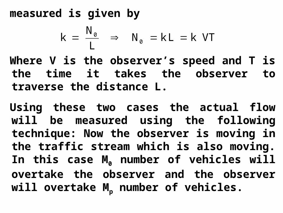
measured is given by

Where V is the observer’s speed and T is the time it takes the observer to traverse the distance L.

Using these two cases the actual flow will be measured using the following technique: Now the observer is moving in the traffic stream which is also moving. In this case M0 number of vehicles will overtake the observer and the observer will overtake Mp number of vehicles.

T V k L k N L

N k 0

0

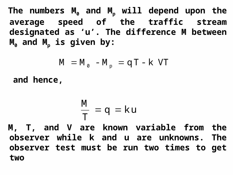
The numbers M0 and Mp will depend upon the average speed of the traffic stream designated as ‘u’. The difference M between M0 and Mp is given by:

and hence,

M, T, and V are known variable from the observer while k and u are unknowns. The observer test must be run two times to get two

T V k - T q M - M M p0

u k q T

M

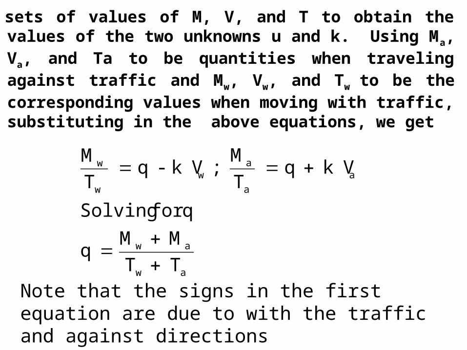
sets of values of M, V, and T to obtain the values of the two unknowns u and k. Using Ma, Va, and Ta to be quantities when traveling against traffic and Mw, Vw, and Tw to be the corresponding values when moving with traffic, substituting in the above equations, we get

aw

aw

a

a

aw

w

w

T T

M M q

q for Solving

Vk q T

M ; Vk - q

T

M

Note that the signs in the first equation are due to with the traffic and against directions

Traffic FlowAnil Kantak

•Shock Waves Traffic: Assume that roadway has uniform traffic with uniform spaces and velocities of the vehicles.

•Suppose a truck slows down to 10 mph all of a sudden.

• Assuming that vehicles are not allowed to overtake the truck, the next vehicle will try to slow down in a safe deceleration and come close to the safe distance and follow the truck with 10 mph speed.

•With time, a moving platoon of vehicles traveling at 10 mph will form behind the truck.

19

Anil Kantak

•In front of the truck road is clear and behind the last vehicle in the platoon the vehicles are going at the normal speed of the roadway. As the time passes, other vehicles have caught up with the platoon and it grows incessantly.

•Suppose the truck either exists the roadway or speed up to the usual speed of the roadway.

•Then next car will speed at a safe acceleration and keep a safe distance between it and the car ahead. Next car would do the same etc. If this persisted for sufficient time then roadway will return to its normal speed.

•This effect is called the shock wave. Traffic Flow 20

Anil Kantak

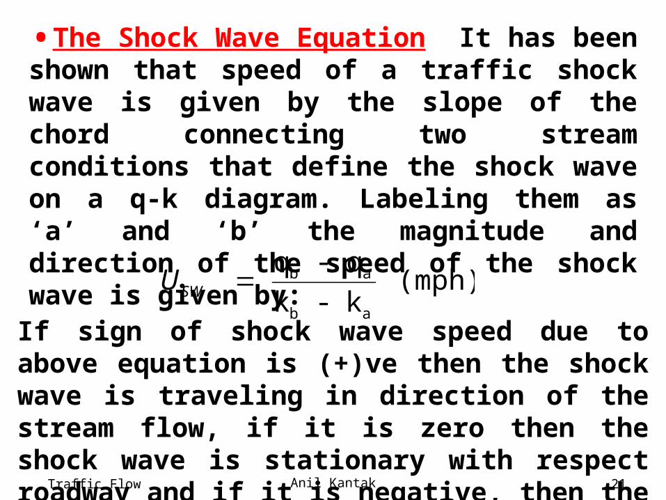
•The Shock Wave Equation It has been shown that speed of a traffic shock wave is given by the slope of the chord connecting two stream conditions that define the shock wave on a q-k diagram. Labeling them as ‘a’ and ‘b’ the magnitude and direction of the speed of the shock wave is given by:

(mph) k - k

q - q

ab

abSWU

If sign of shock wave speed due to above equation is (+)ve then the shock wave is traveling in direction of the stream flow, if it is zero then the shock wave is stationary with respect roadway and if it is negative, then the shock Traffic Flow 21

Anil Kantak

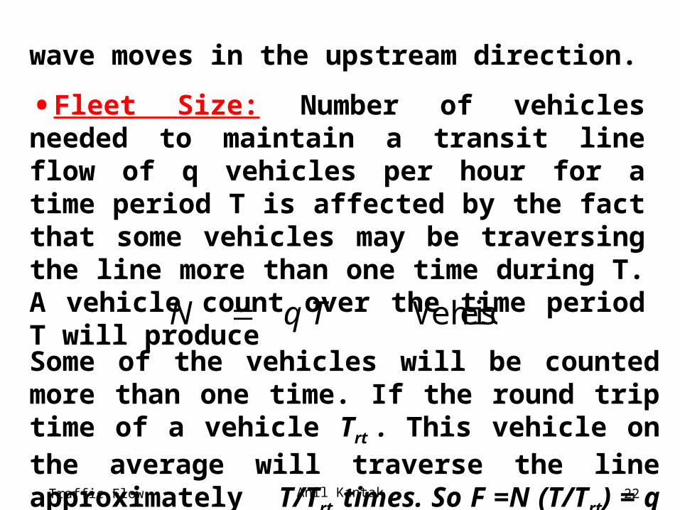
wave moves in the upstream direction.

•Fleet Size: Number of vehicles needed to maintain a transit line flow of q vehicles per hour for a time period T is affected by the fact that some vehicles may be traversing the line more than one time during T. A vehicle count over the time period T will produce

es Vehicl q TN Some of the vehicles will be counted more than one time. If the round trip time of a vehicle Trt . This vehicle on the average will traverse the line approximately T/Trt .times. So F =N (T/Trt) = q Trt

Traffic Flow 22

Anil Kantak

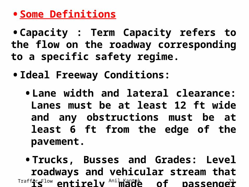
•Some Definitions

•Capacity : Term Capacity refers to the flow on the roadway corresponding to a specific safety regime.

•Ideal Freeway Conditions:

• Lane width and lateral clearance: Lanes must be at least 12 ft wide and any obstructions must be at least 6 ft from the edge of the pavement.

• Trucks, Busses and Grades: Level roadways and vehicular stream that is entirely made of passenger cars.

Traffic Flow 23

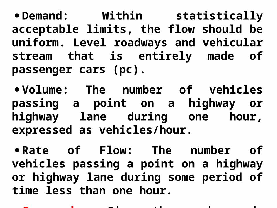
•Demand: Within statistically acceptable limits, the flow should be uniform. Level roadways and vehicular stream that is entirely made of passenger cars (pc).

•Volume: The number of vehicles passing a point on a highway or highway lane during one hour, expressed as vehicles/hour.

•Rate of Flow: The number of vehicles passing a point on a highway or highway lane during some period of time less than one hour.

•Conversion: Since the roadways do not have only passenger cars, a formula is needed to

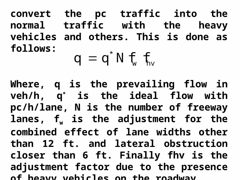
convert the pc traffic into the normal traffic with the heavy vehicles and others. This is done as follows:

hvw* f f N q q

Where, q is the prevailing flow in veh/h, q* is the ideal flow with pc/h/lane, N is the number of freeway lanes, fw is the adjustment for the combined effect of lane widths other than 12 ft. and lateral obstruction closer than 6 ft. Finally fhv is the adjustment factor due to the presence of heavy vehicles on the roadway.

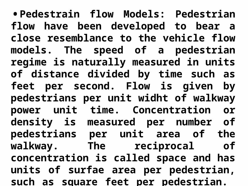
•Pedestrain flow Models: Pedestrian flow have been developed to bear a close resemblance to the vehicle flow models. The speed of a pedestrian regime is naturally measured in units of distance divided by time such as feet per second. Flow is given by pedestrians per unit widht of walkway power unit time. Concentration or density is measured per number of pedestrians per unit area of the walkway. The reciprocal of concentration is called space and has units of surfae area per pedestrian, such as square feet per pedestrian. The fundamental relationship q = u k is valid here too.