BIS WORKING PAPERS

No 93 – October 2000

TRADING VOLUMES, VOLATILITY

AND SPREADS IN FOREIGN EXCHANGE MARKETS:

EVIDENCE FROM EMERGING MARKET COUNTRIES

by

Gabriele Galati

BANK FOR INTERNATIONAL SETTLEMENTSMonetary and Economic Department

Basel, Switzerland

BIS Working Papers are written by members of the Monetary and Economic Department of the Bank forInternational Settlements, and from time to time by other economists, and are published by the Bank. The papersare on subjects of topical interest and are technical in character. The views expressed in them are those of theirauthors and not necessarily the views of the BIS.

Copies of publications are available from:

Bank for International SettlementsInformation, Press & Library ServicesCH-4002 Basel, Switzerland

Fax: +41 61 / 280 91 00 and +41 61 / 280 81 00

This publication is available on the BIS website (www.bis.org).

© Bank for International Settlements 2000.All rights reserved. Brief excerpts may be reproduced or translated provided the source is stated.

ISSN 1020-0959

BIS WORKING PAPERS

No 93 – October 2000

TRADING VOLUMES, VOLATILITY

AND SPREADS IN FOREIGN EXCHANGE MARKETS:

EVIDENCE FROM EMERGING MARKET COUNTRIES

by

Gabriele Galati*

Abstract

This paper provides empirical evidence on the relationship between tradingvolumes, volatility and bid-ask spreads in foreign exchange markets. It uses a newdata set that includes daily data on trading volumes for the dollar exchange rates ofseven currencies from emerging market countries. The sample period is 1 January1998 to 30 June 1999. The results are broadly consistent with the findings of theliterature that used futures volumes as proxies for total foreign exchange trading. Ifind that in most cases unexpected trading volumes and volatility are positivelycorrelated, suggesting that both are driven by the arrival of public information, aspredicted by the mixture of distributions hypothesis. I also find that the correlationbetween trading volumes and volatility is positive during “normal” periods butturns negative when volatility increases sharply. Finally, the results suggest thatvolatility and spreads are positively correlated, as suggested by inventory costmodels. However, contrary to the prediction of these models, I do not find evidenceof a significant impact of unexpected trading volumes on spreads.

* I thank Javiera Aguilar, Claudio Borio, Alain Chaboud, Stefan Gerlach, Bob McCauley, Eli Remolona andKostas Tsatsaronis for helpful comments and Florence Béranger and Anna Cobau for research assistance.

Contents

1. Introduction ................................................................................................................... 1

2. Literature review ........................................................................................................... 2

3. The data ......................................................................................................................... 5

Exchange rates .................................................................................................... 5

Volatility ............................................................................................................. 6

Trading volumes ................................................................................................. 7

Spreads ................................................................................................................ 9

4. Volumes, volatility and spreads .................................................................................... 10

Trading volumes and volatility ........................................................................... 10

Trading volumes and bid-ask spreads ................................................................. 13

5. Conclusions ................................................................................................................... 13

6. Tables and graphs ......................................................................................................... 15

References .................................................................................................................................... 32

1

1. Introduction

This paper looks at the relationship between trading volumes, volatility and bid-ask spreads in foreign

exchange markets. A number of studies on the microstructure of foreign exchange markets have

looked at this issue from both a theoretical and an empirical point of view. From a policy perspective,

the issue is important because of its implications for the analysis of market liquidity and its

relationship with risk. Broadly speaking, a market can be considered to be liquid when large

transactions can be executed with a small impact on prices (BIS (1999a)). In practice, however, no

data are available that allow this definition of foreign exchange market liquidity to be measured

directly. Instead, trading volumes or bid-ask spreads are frequently used as indirect measures.

Volatility is often considered as a measure of risk.

This paper uses a new data set that for the first time matches daily data on trading volumes, volatility

and spreads. The data set covers the dollar exchange rates of seven currencies from emerging market

countries: the Colombian peso, the Mexican peso, the Brazilian real, the Indian rupee, the Indonesian

rupiah, the Israeli shekel and the South African rand. The data cover the period from January 1998 to

June 1999 and use total turnover in the local market. Since there is not much offshore trading in these

currencies, local transaction volumes are fairly representative of total trading. In order to allow a

comparison with foreign exchange markets in industrial countries and with the results from previous

studies, the paper also looks at trading volumes from the Tokyo inter-dealer yen/dollar market.

Finally, for the Mexican peso, data from a fairly active currency futures market on the Chicago

Mercantile Exchange were also obtained. These data allow a direct comparison of volumes on foreign

exchange and futures markets.

An important drawback of empirical studies in this area is that good data on foreign exchange trading

volumes have so far not been available at high frequencies. The most comprehensive source of

information on trading in foreign exchange markets, the triennial Central Bank Survey of Foreign

Exchange and Derivatives Market Activity published by the BIS, for example, does not provide much

information on the time series behaviour of trading volumes. Researchers have therefore looked at

alternative data sources to find proxies for foreign exchange market turnover. By using actual spot

market trading volumes, this paper is for the first time able to fill this important gap in the literature.

The empirical microstructure literature has typically found a positive correlation between volumes and

volatility. A theoretical explanation of this finding is that volume and volatility are both driven by a

common, unobservable factor, which is determined by the arrival of new information. This theory,

also known as the mixture of distributions hypothesis, predicts that volatility will move together with

unexpected trading volumes. A further common finding of the literature is that volume and spreads are

2

positively correlated. The explanation provided by microstructure theory is that bid-ask spreads are

determined inter alia by inventory costs, which widen when exchange rate volatility increases.

Through the mixture of distributions hypothesis, this also establishes a positive link between

unexpected volumes and spreads.

A main finding of this paper is that in most cases unexpected trading volumes and volatility are

positively correlated, suggesting that they both react to the arrival of new information, as the mixture

of distributions hypothesis predicts. This result is in line with the findings of the literature that relies

on futures data. The markets for the Mexican peso and the real, however, provide important

exceptions. In these two cases, the relationship between unexpected volumes and volatility is negative

but not statistically significant. I provide evidence that this result is driven by the incidence of periods

of turbulence and argue that the correlation between trading volumes and volatility may be positive

during “normal” times but negative during periods of stress. I also find evidence of a positive

correlation between volatility and spreads, as suggested by inventory cost models. However, the

results do not show a significant impact of trading volumes on spreads.

The remainder of the paper is organised as follows. Section 2 reviews the main contributions to the

literature on the relationship between trading volumes, volatility and spreads. Section 3 describes the

data set that is used. In Section 4, I present some descriptive evidence on the relationship between

volumes, volatility and spreads. I then use regression analysis to test whether the mixture of

distributions hypothesis holds in foreign exchange markets. Section 5 concludes.

2. Literature review

There is extensive literature on the relationship between trading volumes and volatility in financial

markets. Karpoff (1987) provides a good overview of the early literature. Most of the research has

focused on stock markets and futures markets, for which data on volumes are more easily available.

An important finding is that trading volume and price variability are positively correlated at different

frequencies. The coefficient is highest for contemporaneous correlations. However, it does not always

appear to be very sizeable. Evidence was found by Harris (1986) and Richardson et al (1987) for stock

markets and by Cornell (1981) for commodity futures.

The empirical work on foreign exchange markets has suffered from the problem that good data on

trading volumes are not easily available for foreign exchange markets since, unlike equity markets,

they are for the most part decentralised. Different data sources were used to describe the time series

behaviour of trading volumes.1 Many studies used data on futures contracts, which can be easily

1 A good overview of the characteristics of data sets used in the literature can be found in Lyons (2000).

3

obtained, to proxy for interbank trading volumes. Studies that have found a positive correlation

between volumes and volatility in these markets include Grammatikos and Saunders (1986), Batten

and Bhar (1993) and Jorion (1996). An obvious drawback of these data sets is that trading in futures is

very small compared to OTC volumes (Dumas (1996)). In the first quarter of 1998, for example, total

turnover of currency futures traded on organised exchanges amounted to roughly $70 billion (BIS

(1998)), compared to total OTC turnover in spot, forward and swap markets of about $1,500 billion

(BIS (1999b)). While these two markets may still be closely linked through arbitrage (Lyons (2000)),

little evidence is available on this link.

A widely used source of information on foreign exchange trading, the triennial Central Bank Survey of

Foreign Exchange and Derivatives Market Activity published by the BIS, provides extensive cross

sectional information but very little information on the time series behaviour of turnover. Hartmann

(1998b) makes efficient use of these data by combining a large cross section of exchange rates taken

from the BIS triennial survey with two time series observations into a panel, but still faces the problem

of having limited time series information.

An alternative source of information is the Bank of Japan’s data set on brokered transactions in the

Tokyo yen/dollar market, which has been used by Wei (1994) and Hartmann (1999). A problem with

these data is that they represent only a fraction (about one sixth) of total turnover in the Tokyo

yen/dollar market and no more than 5% of the global yen/dollar market.

A number of papers have used the frequency of indicative quotes posted by Reuters on its FXFX page

as a proxy for trading volumes.2 However, these quotes do not represent actual trades and it is not

possible to infer from a quote for which volume it is given. Spreads that are quoted on the Reuters

screen are generally far from actual traded spreads.3 Moreover, it is common for banks that act as data

providers to programme an automated data input, eg by having a particular quote entered at regular

time intervals. This is especially true for smaller banks that may have an interest in quoting prices in

order to advertise their presence in a particular market segment. Finally, when an important event

occurs, traders are likely to act and trade rather than entering data for Reuters. Hence, Reuters tick

frequency may be low at times of high trading activity and high when markets are calm. The

relationship between quote frequency and actual trading activity is therefore likely to be quite noisy.

A fruitful approach has been to look at high-frequency data on actual transactions in the OTC market.

One such data set, used by Lyons (1995), covers all transactions that a foreign exchange dealer in New

York entered with other dealers in one week in 1992. Goodhart et al (1996) analyse data on

electronically brokered inter-dealer transactions that occurred on one day in 1993. While these data

2 See for example, Goodhart and Figliuoli (1991) and Bollerslev and Domowitz (1993).

3 See also Hartmann (1998a).

4

provide a wealth of information, including information on the direction of order flows, they

necessarily cover only a limited segment of foreign exchange markets and span a relatively short time

period.

Different theoretical explanations have been offered for the co-movement of trading volumes and

volatility. Early work was based on models of “sequential information arrival” (Copeland

(1976, 1977)), according to which information reaches one market participant at a time. As that agent

reacts to the arrival of news, his demand curve will shift, thereby leading to a positive correlation

between volume and volatility. An alternative explanation of the volume-volatility correlation is based

on the “mixture of distributions hypothesis” first proposed by Clark (1973). According to this

hypothesis, volume and volatility are both driven by a common, unobservable factor. This factor

reflects the arrival of new public information and determines a positive correlation between

unexpected turnover and unexpected volatility. Tauchen and Pitts (1983) show that volume and

volatility can co-move for two reasons. First, as the number of traders grows, market prices become

less volatile. Second, given the number of traders, an increase in volume reflects greater disagreement

among traders and hence leads to higher volatility. This link is stronger when new information arrives

at a faster rate. In a recent paper, Melvin and Yin (2000) investigated the relationship between the

arrival of new public information, the quoting frequency and the volatility of dollar/yen and

dollar/mark exchange rates. They analysed intra-day data taken from Reuters screens on indicative

quotes and news headlines related to the United States, Germany or Japan for the period 1 December

1993 to 26 April 1995. They found that the amount of information arriving on a particular hour of a

particular day of the week is positively related to the amount of quoting activity and exchange rate

volatility.

Models that explain bid-ask spreads in terms of inventory costs establish a link between bid-ask

spreads, volatility and trading volumes. One determinant of inventory costs is the cost of maintaining

open positions, which is positively related to price risk.4 According to this view, exchange rate

volatility increases price risk and thereby pushes up spreads. Supporting evidence is provided by

Bessembinder (1994), Bollerslev and Melvin (1994) and Hartmann (1999), who found a positive

correlation between spreads and expected volatility measured by GARCH forecasts.

A second determinant of inventory costs is trading activity. Trading volumes can have a different

impact on spreads depending on whether they are expected or unexpected. Expected trading volumes

should be negatively correlated with spreads to the extent that they reflect economies of scale and are

associated with higher competition among market-makers (Cornell (1978)). By contrast, unexpected

4 The microstructure literature analyses two other types of costs: order processing costs (ie costs of providing liquidity

services) and asymmetric information costs (Bessembinder (1994), Jorion (1996) Hartmann (1999), Lyons (2000)). Orderprocessing costs are arguably small in foreign exchange markets (Jorion (1996)). Recent research (Lyons (2000)) stressesthe importance of asymmetric information costs.

5

trading volumes should have a positive impact on spreads to the extent that they reflect the arrival of

news.

3. The data

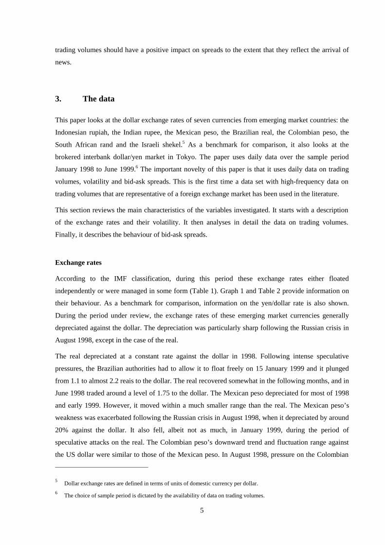
This paper looks at the dollar exchange rates of seven currencies from emerging market countries: the

Indonesian rupiah, the Indian rupee, the Mexican peso, the Brazilian real, the Colombian peso, the

South African rand and the Israeli shekel.5 As a benchmark for comparison, it also looks at the

brokered interbank dollar/yen market in Tokyo. The paper uses daily data over the sample period

January 1998 to June 1999.6 The important novelty of this paper is that it uses daily data on trading

volumes, volatility and bid-ask spreads. This is the first time a data set with high-frequency data on

trading volumes that are representative of a foreign exchange market has been used in the literature.

This section reviews the main characteristics of the variables investigated. It starts with a description

of the exchange rates and their volatility. It then analyses in detail the data on trading volumes.

Finally, it describes the behaviour of bid-ask spreads.

Exchange rates

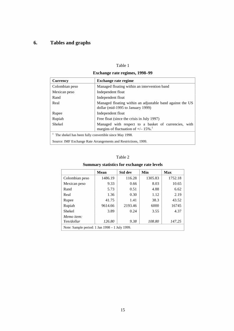
According to the IMF classification, during this period these exchange rates either floated

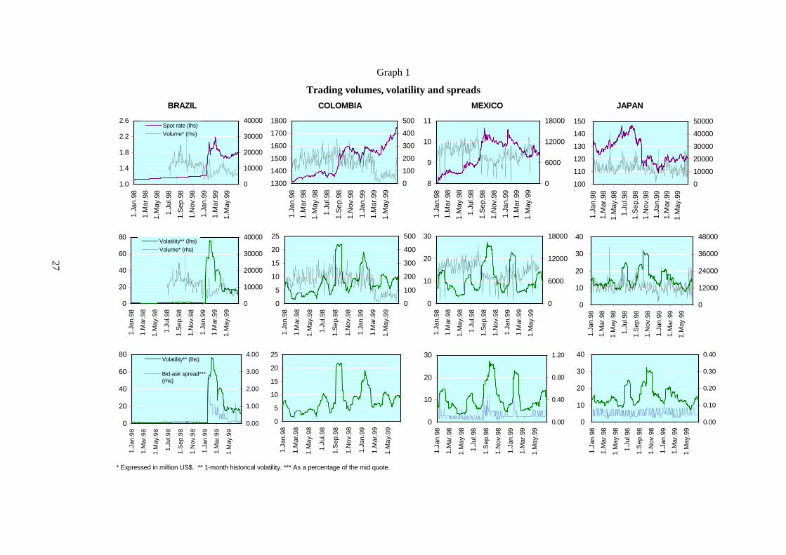
independently or were managed in some form (Table 1). Graph 1 and Table 2 provide information on

their behaviour. As a benchmark for comparison, information on the yen/dollar rate is also shown.

During the period under review, the exchange rates of these emerging market currencies generally

depreciated against the dollar. The depreciation was particularly sharp following the Russian crisis in

August 1998, except in the case of the real.

The real depreciated at a constant rate against the dollar in 1998. Following intense speculative

pressures, the Brazilian authorities had to allow it to float freely on 15 January 1999 and it plunged

from 1.1 to almost 2.2 reais to the dollar. The real recovered somewhat in the following months, and in

June 1998 traded around a level of 1.75 to the dollar. The Mexican peso depreciated for most of 1998

and early 1999. However, it moved within a much smaller range than the real. The Mexican peso’s

weakness was exacerbated following the Russian crisis in August 1998, when it depreciated by around

20% against the dollar. It also fell, albeit not as much, in January 1999, during the period of

speculative attacks on the real. The Colombian peso’s downward trend and fluctuation range against

the US dollar were similar to those of the Mexican peso. In August 1998, pressure on the Colombian

5 Dollar exchange rates are defined in terms of units of domestic currency per dollar.

6 The choice of sample period is dictated by the availability of data on trading volumes.

6

currency stepped up, inducing the authorities to widen the intervention band by 9%, effectively

devaluing the currency. The peso came under renewed pressure in January and March 1999. In June

1999, it depreciated by about 20%.

The Indian rupee’s behaviour was characterised by periods of stability followed by marked downward

movements, notably in May 1998. The Indonesian rupiah fell sharply in January and July 1998. Its

volatility declined in 1999 but still remained very high.

The South African rand depreciated markedly against the dollar around the time of the Russian crisis

in summer 1998. In the second half of the year it recouped part of its losses but in 1999 trended down

again. In 1998, the shekel followed a slightly depreciating trend against the dollar. It fell by 20% in

October 1998 but stabilised in the following weeks.

Unlike the exchange rates of the seven emerging market currencies, the movements of the dollar/yen

rate were much smoother over most of the sample period. However, in October 1998 the dollar fell

sharply and lost about 20% against the yen in a few days.

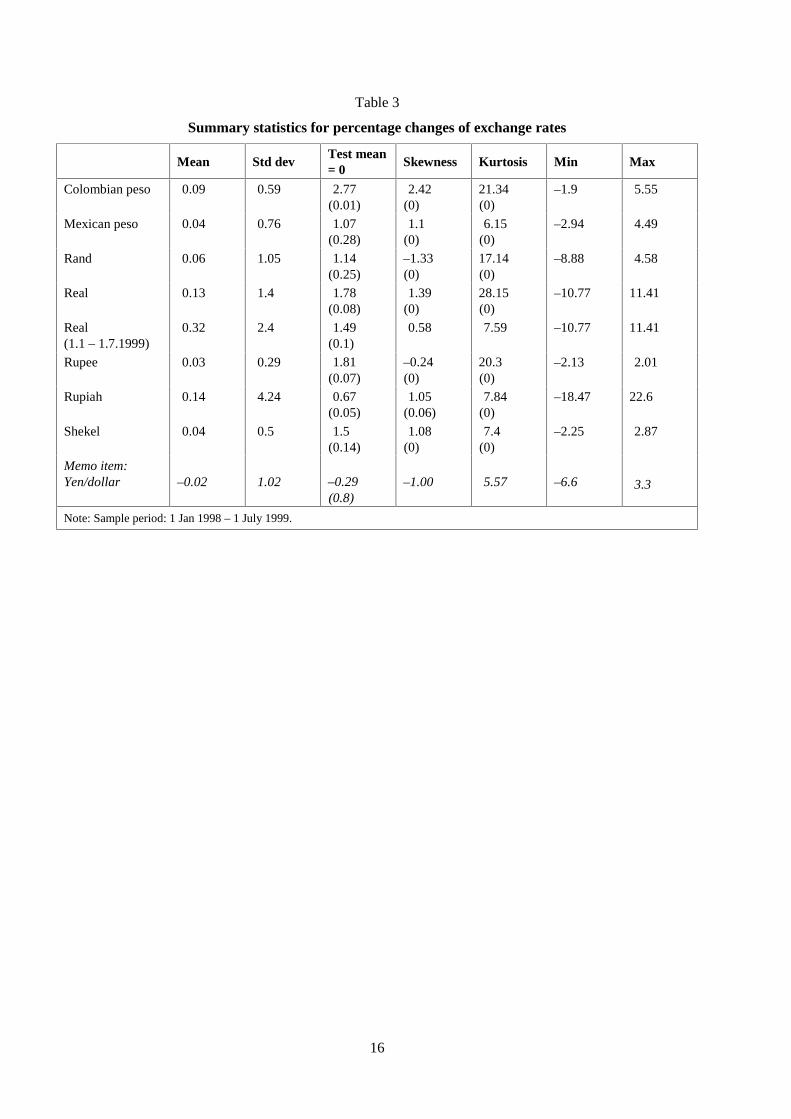
Graph 3 and Table 3 report information on the percentage exchange rate changes for the seven

currencies. For the real, statistics are also presented separately for the period January–June 1999,

during which it floated. Between January 1998 and June 1999, the average daily percentage change of

most of the currencies was significantly positive, with the exception of the Colombian peso and the

rupee. Their standard deviation ranged between 0.29 for the rupee and 4.24 for the rupiah. Over the

same period, the standard deviation of the yen/dollar rate was close to 1. Most exchange rate changes

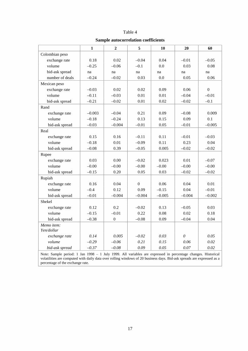
exhibited positive skewness consistently with their downward trend, and leptokurtosis. Table 4

suggests that the exchange rate changes exhibited very little persistence.

Volatility

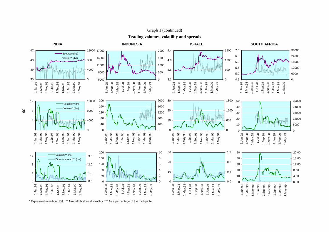
Graph 1 shows the historical volatility of the seven exchange rates computed over moving windows of

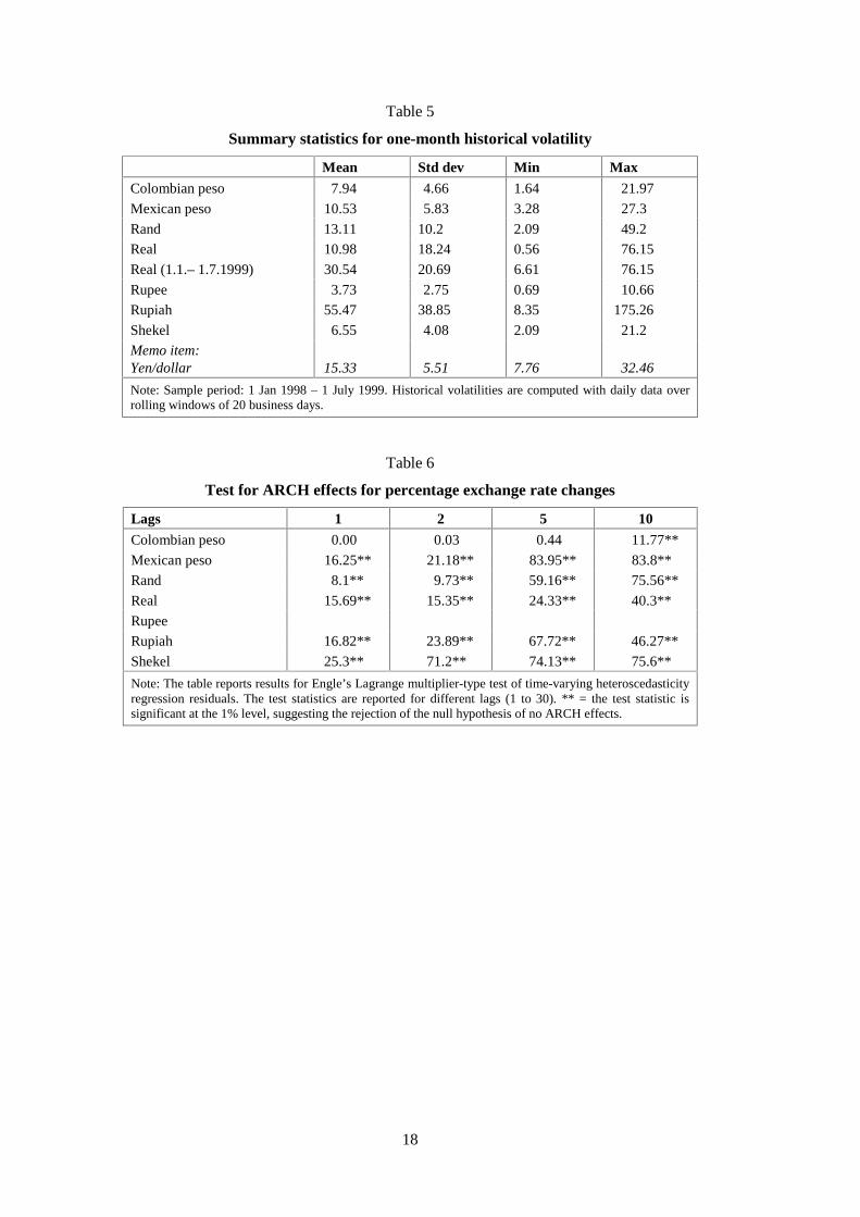
one month. Summary statistics are reported in Table 5. In terms of their volatility, the seven exchange

rates can be divided into two groups. The real and the rupiah experienced sharp volatility spikes and

were characterised by very high average volatility. By contrast, the historical volatilities of the rupee,

the shekel and the Colombian peso remained quite low, averaging less than 8%. The rand’s volatility

was relatively low on average, but it spiked at about 50%.

Table 5 shows that the volatility of the yen/dollar exchange rate during the same period averaged 15%.

This is much less than the volatility of the real or the rupiah vis-à-vis the dollar, but more than the

volatility of the other five exchange rates in this data set.

A finding that is common for exchange rates and other asset prices is the existence of volatility

clustering, ie the fact that periods of persistent turbulence are followed by periods of relative calm. In

7

the finance literature, this phenomenon has typically been described by some ARCH-type models.

Tests for ARCH-type effects presented in Table 6 suggest that the exchange rates under investigation

– with the possible exception of the Colombian peso – exhibit some ARCH-type behaviour. This

behaviour seems to be fairly well captured by a GARCH(1,1) model.

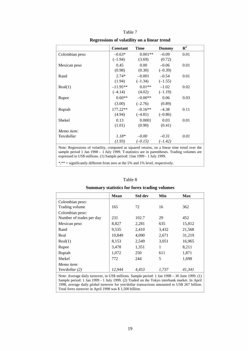
Finally, Table 7 presents evidence that, for half of the exchange rates, volatility follows a time trend.

The trend is positive for the Colombian peso and the real and negative for the rupee and the rupiah.

There is no evidence of weekend effects.

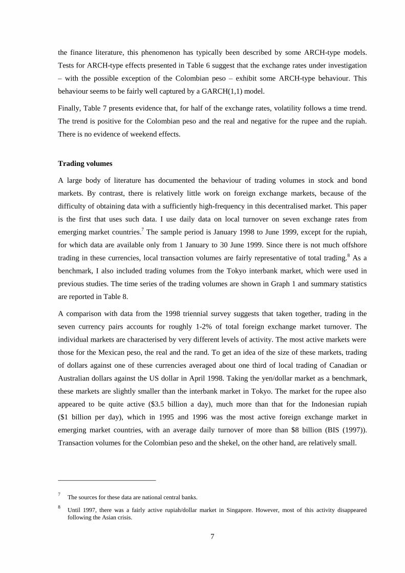
Trading volumes

A large body of literature has documented the behaviour of trading volumes in stock and bond

markets. By contrast, there is relatively little work on foreign exchange markets, because of the

difficulty of obtaining data with a sufficiently high-frequency in this decentralised market. This paper

is the first that uses such data. I use daily data on local turnover on seven exchange rates from

emerging market countries.7 The sample period is January 1998 to June 1999, except for the rupiah,

for which data are available only from 1 January to 30 June 1999. Since there is not much offshore

trading in these currencies, local transaction volumes are fairly representative of total trading.8 As a

benchmark, I also included trading volumes from the Tokyo interbank market, which were used in

previous studies. The time series of the trading volumes are shown in Graph 1 and summary statistics

are reported in Table 8.

A comparison with data from the 1998 triennial survey suggests that taken together, trading in the

seven currency pairs accounts for roughly 1-2% of total foreign exchange market turnover. The

individual markets are characterised by very different levels of activity. The most active markets were

those for the Mexican peso, the real and the rand. To get an idea of the size of these markets, trading

of dollars against one of these currencies averaged about one third of local trading of Canadian or

Australian dollars against the US dollar in April 1998. Taking the yen/dollar market as a benchmark,

these markets are slightly smaller than the interbank market in Tokyo. The market for the rupee also

appeared to be quite active ($3.5 billion a day), much more than that for the Indonesian rupiah

($1 billion per day), which in 1995 and 1996 was the most active foreign exchange market in

emerging market countries, with an average daily turnover of more than $8 billion (BIS (1997)).

Transaction volumes for the Colombian peso and the shekel, on the other hand, are relatively small.

7 The sources for these data are national central banks.

8 Until 1997, there was a fairly active rupiah/dollar market in Singapore. However, most of this activity disappeared

following the Asian crisis.

8

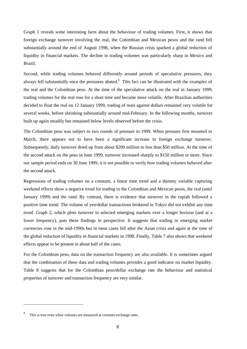
Graph 1 reveals some interesting facts about the behaviour of trading volumes. First, it shows that

foreign exchange turnover involving the real, the Colombian and Mexican pesos and the rand fell

substantially around the end of August 1998, when the Russian crisis sparked a global reduction of

liquidity in financial markets. The decline in trading volumes was particularly sharp in Mexico and

Brazil.

Second, while trading volumes behaved differently around periods of speculative pressures, they

always fell substantially once the pressures abated.9 This fact can be illustrated with the examples of

the real and the Colombian peso. At the time of the speculative attack on the real in January 1999,

trading volumes for the real rose for a short time and became more volatile. After Brazilian authorities

decided to float the real on 12 January 1999, trading of reais against dollars remained very volatile for

several weeks, before shrinking substantially around mid-February. In the following months, turnover

built up again steadily but remained below levels observed before the crisis.

The Colombian peso was subject to two rounds of pressure in 1999. When pressure first mounted in

March, there appears not to have been a significant increase in foreign exchange turnover.

Subsequently, daily turnover dried up from about $200 million to less than $50 million. At the time of

the second attack on the peso in June 1999, turnover increased sharply to $150 million or more. Since

our sample period ends on 30 June 1999, it is not possible to verify how trading volumes behaved after

the second attack.

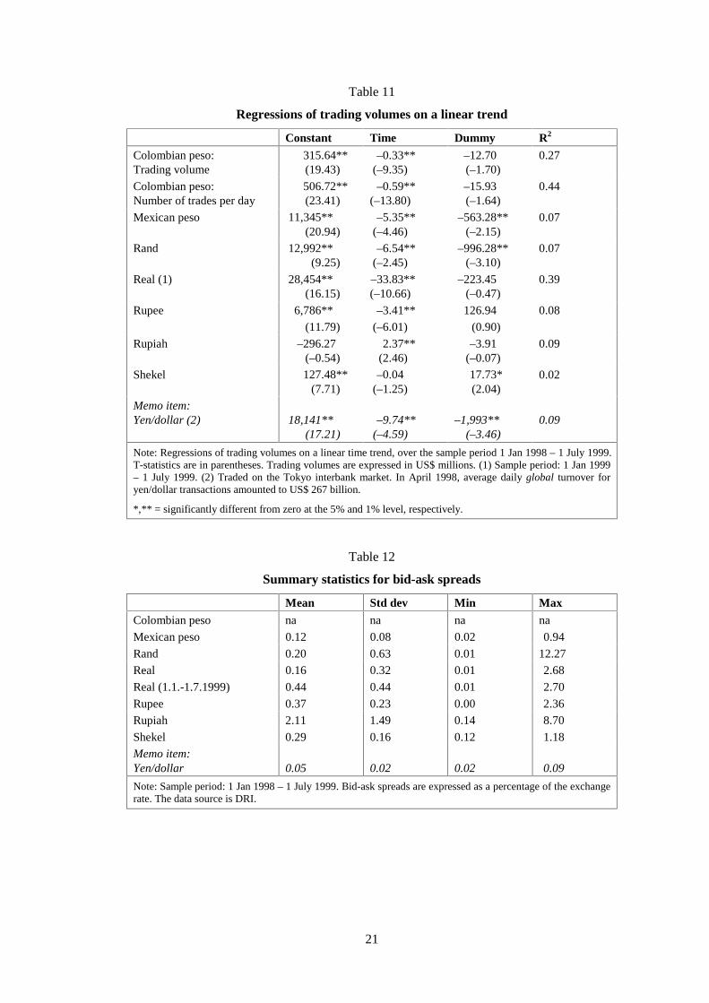
Regressions of trading volumes on a constant, a linear time trend and a dummy variable capturing

weekend effects show a negative trend for trading in the Colombian and Mexican pesos, the real (until

January 1999) and the rand. By contrast, there is evidence that turnover in the rupiah followed a

positive time trend. The volume of yen/dollar transactions brokered in Tokyo did not exhibit any time

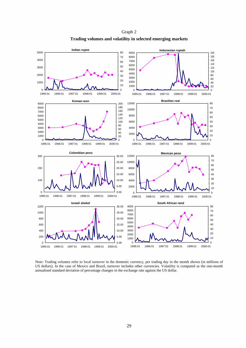
trend. Graph 2, which plots turnover in selected emerging markets over a longer horizon (and at a

lower frequency), puts these findings in perspective. It suggests that trading in emerging market

currencies rose in the mid-1990s but in most cases fell after the Asian crisis and again at the time of

the global reduction of liquidity in financial markets in 1998. Finally, Table 7 also shows that weekend

effects appear to be present in about half of the cases.

For the Colombian peso, data on the transaction frequency are also available. It is sometimes argued

that the combination of these data and trading volumes provides a good indicator on market liquidity.

Table 8 suggests that for the Colombian peso/dollar exchange rate the behaviour and statistical

properties of turnover and transaction frequency are very similar.

9 This is true even when volumes are measured at constant exchange rates.

9

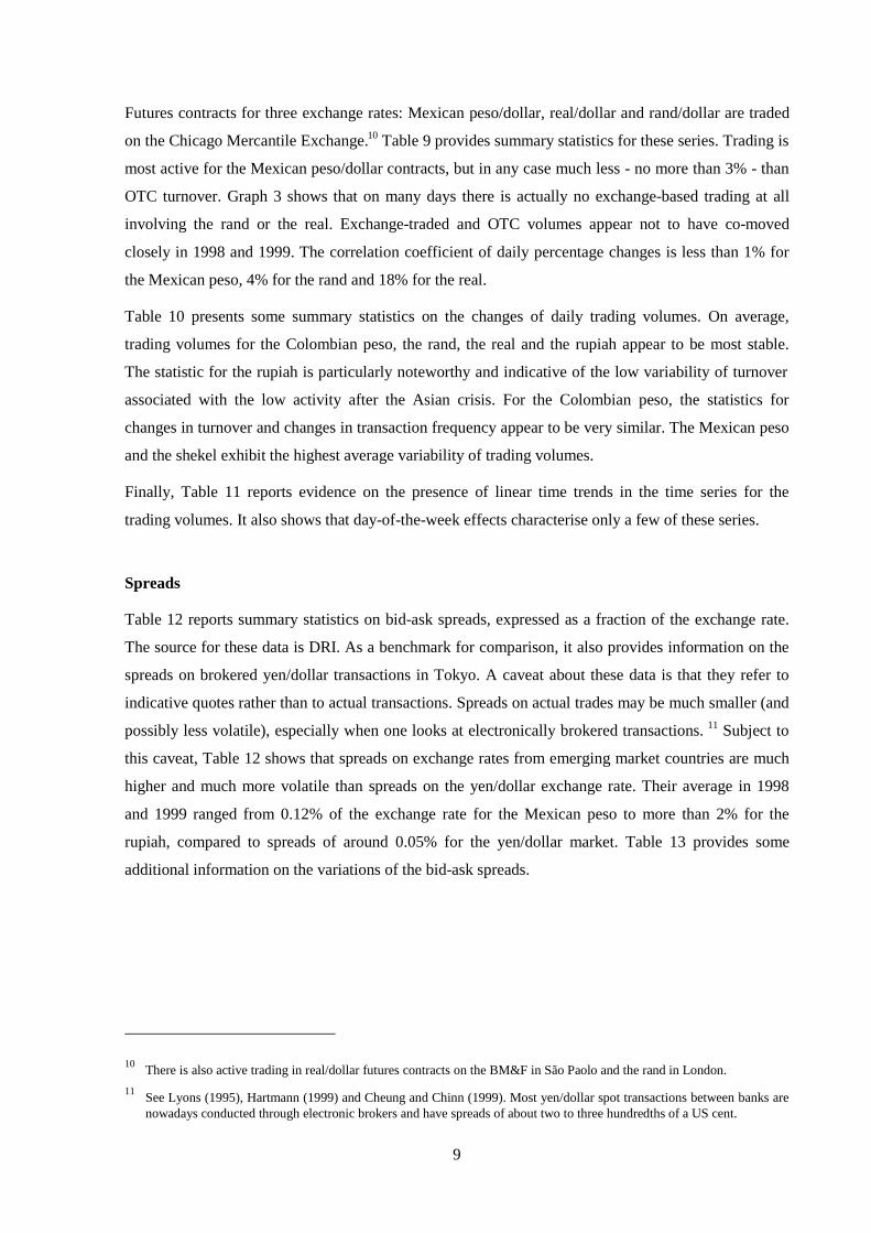
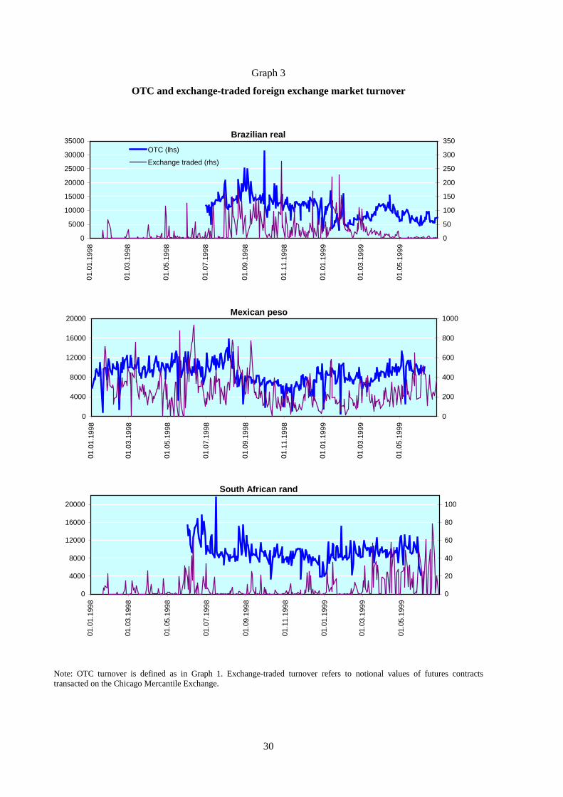
Futures contracts for three exchange rates: Mexican peso/dollar, real/dollar and rand/dollar are traded

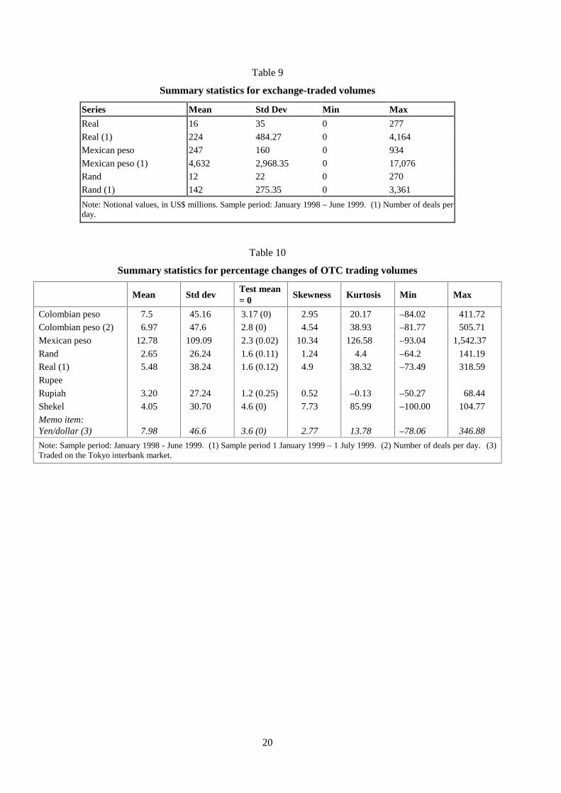
on the Chicago Mercantile Exchange.10 Table 9 provides summary statistics for these series. Trading is

most active for the Mexican peso/dollar contracts, but in any case much less - no more than 3% - than

OTC turnover. Graph 3 shows that on many days there is actually no exchange-based trading at all

involving the rand or the real. Exchange-traded and OTC volumes appear not to have co-moved

closely in 1998 and 1999. The correlation coefficient of daily percentage changes is less than 1% for

the Mexican peso, 4% for the rand and 18% for the real.

Table 10 presents some summary statistics on the changes of daily trading volumes. On average,

trading volumes for the Colombian peso, the rand, the real and the rupiah appear to be most stable.

The statistic for the rupiah is particularly noteworthy and indicative of the low variability of turnover

associated with the low activity after the Asian crisis. For the Colombian peso, the statistics for

changes in turnover and changes in transaction frequency appear to be very similar. The Mexican peso

and the shekel exhibit the highest average variability of trading volumes.

Finally, Table 11 reports evidence on the presence of linear time trends in the time series for the

trading volumes. It also shows that day-of-the-week effects characterise only a few of these series.

Spreads

Table 12 reports summary statistics on bid-ask spreads, expressed as a fraction of the exchange rate.

The source for these data is DRI. As a benchmark for comparison, it also provides information on the

spreads on brokered yen/dollar transactions in Tokyo. A caveat about these data is that they refer to

indicative quotes rather than to actual transactions. Spreads on actual trades may be much smaller (and

possibly less volatile), especially when one looks at electronically brokered transactions. 11 Subject to

this caveat, Table 12 shows that spreads on exchange rates from emerging market countries are much

higher and much more volatile than spreads on the yen/dollar exchange rate. Their average in 1998

and 1999 ranged from 0.12% of the exchange rate for the Mexican peso to more than 2% for the

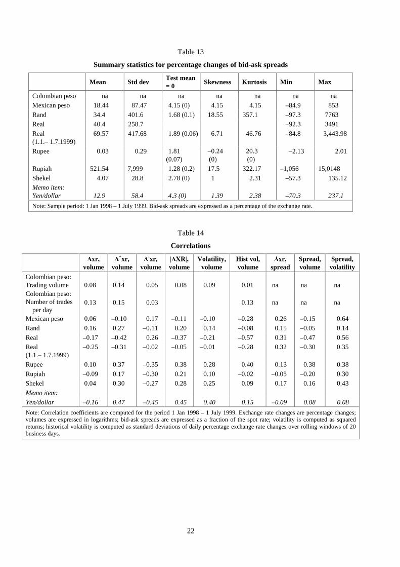
rupiah, compared to spreads of around 0.05% for the yen/dollar market. Table 13 provides some

additional information on the variations of the bid-ask spreads.

10 There is also active trading in real/dollar futures contracts on the BM&F in São Paolo and the rand in London.

11 See Lyons (1995), Hartmann (1999) and Cheung and Chinn (1999). Most yen/dollar spot transactions between banks are

nowadays conducted through electronic brokers and have spreads of about two to three hundredths of a US cent.

10

4. Volumes, volatility and spreads

Trading volumes and volatility

In terms of the contemporaneous correlation between daily foreign exchange turnover and exchange

rate volatility, Table 14 shows positive coefficients for five out of seven emerging market exchange

rates (the dollar exchange rates of the Colombian peso, the rand, the rupee, the rupiah and the shekel).

The correlation is also positive for the yen/dollar rate traded in the Tokyo interbank market. This holds

irrespective of whether exchange rate volatility is measured by absolute values of percentage changes,

squared returns or the standard deviation of daily returns computed over rolling windows of one

month. By contrast, I find a negative correlation for the real and the Mexican peso.

Regressions of volatility on a constant, a time trend, a day-of-the-week dummy and trading volumes

give positive and statistically significant coefficients for all currencies except the real and the Mexican

peso (Table 16). For the Colombian peso, a regression of volatility on the number of deals per day also

gives a positive and statistically significant coefficient. With the exception of the real and the Mexican

peso, these results are consistent with the positive correlation of volatility and volume found for

currency futures (Grammatikos and Saunders (1986), Jorion (1996)).

Table 15 shows that for the Mexican peso, exchange-traded data yield a positive correlation between

volatility and volumes. This result suggests that exchange-traded data may not always be an

appropriate proxy for total interbank trading.

The positive correlation between volumes and volatility found for most of the exchange rates is

unlikely to be a reflection of changes in the number of traders active in these markets. These changes

appear rather to have occurred in the mid-1990s, when banks increasingly moved into emerging

markets, and after the Asian crisis, when the sharp fall in turnover was accompanied by a significant

decline in the number of traders. A more plausible explanation for the positive correlation between

turnover and volatility is that both variables are driven by the arrival of new information.

To test this hypothesis, I split volatility and trading volumes into expected and unexpected

components. I use estimates from a GARCH(1,1) model to describe expected volatility. This model

appears to fit the time series well.12 Ideally, volatility implied in option prices could be used, since

there is evidence that it outperforms GARCH models in providing forecasts of future volatility.13

However, option contracts for currencies of emerging market countries are not very liquid, particularly

after the Asian crisis. The GARCH(1,1) model can be written as:

12 Following a practice common in the literature, the GARCH model is fitted on the entire time series, thus yielding in-

sample forecasts.

11

where Rt is the return, its mean and ht its conditional variance at time t.

In order to measure expected trading volumes, I used the Box-Jenkins analysis to select a

parsimonious time series representation for the volume series, which are taken in logs. Time series

models were fitted on the levels of trading volumes since Augmented Dickey-Fuller tests suggest that

they are stationary. AR models, in most cases of first order, seemed appropriate to represent the

turnover series. These models allow trading volumes to be split into an expected and an unexpected

component.

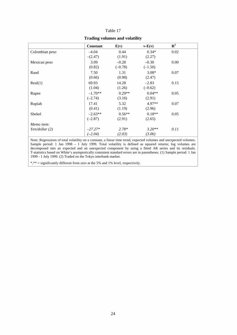
The estimated regression equation takes the following form:

where total volatility R2t+1 is defined as squared returns, and log volumes are decomposed into an

expected component Et(v) and an unexpected component [vt+1-Et(v)] by using a fitted AR series and its

residuals. A linear time trend and a dummy capturing weekend effects are also included.

Equation (2) is then augmented with an expected volatility term ht+1 , which represents the one-step-

ahead conditional return variance from a GARCH(1,1) specification:

Table 17 reports the regression results for equation (3). The coefficient on unexpected turnover is

positive and statistically significant at 1% or 5% in all the regressions for exchange rates from

emerging market countries, except those for the Mexican peso and the real. For these two currencies,

the coefficients are negative but not statistically significant. A positive, significant coefficient is also

found for the yen/dollar rate traded in Tokyo. Except for the Mexican peso and the real, the results

support the idea that information flow drives volatility and volumes, as implied by the mixture of

distributions hypothesis. This result is consistent with the conclusion of the literature that used data on

currency futures (Jorion (1996)). These results are independent of market size: they hold both for the

smallest market (Colombian peso/dollar) and for the biggest market (rand/dollar) in emerging market

13 Jorion (1996).

12

110),,0(~,)1( −− ++=+= tttttt hrhhNrrR βααµ

1541322

1 )]([)()2( +++ +++−++= ttttt wtvEvvER εββββα

154132112

1 )]([)()3( ++++ +++−+++= tttttt wtvEvvEhR εβββββα

12

countries, as well as for the even bigger yen/dollar interbank market in Tokyo. This is consistent with

the finding presented in Batten and Bhar (1993) for futures markets. In contrast to Jorion’s results,

however, expected volumes also have a positive, significant effect on volatility in three cases (the

rupee, the shekel and the yen).

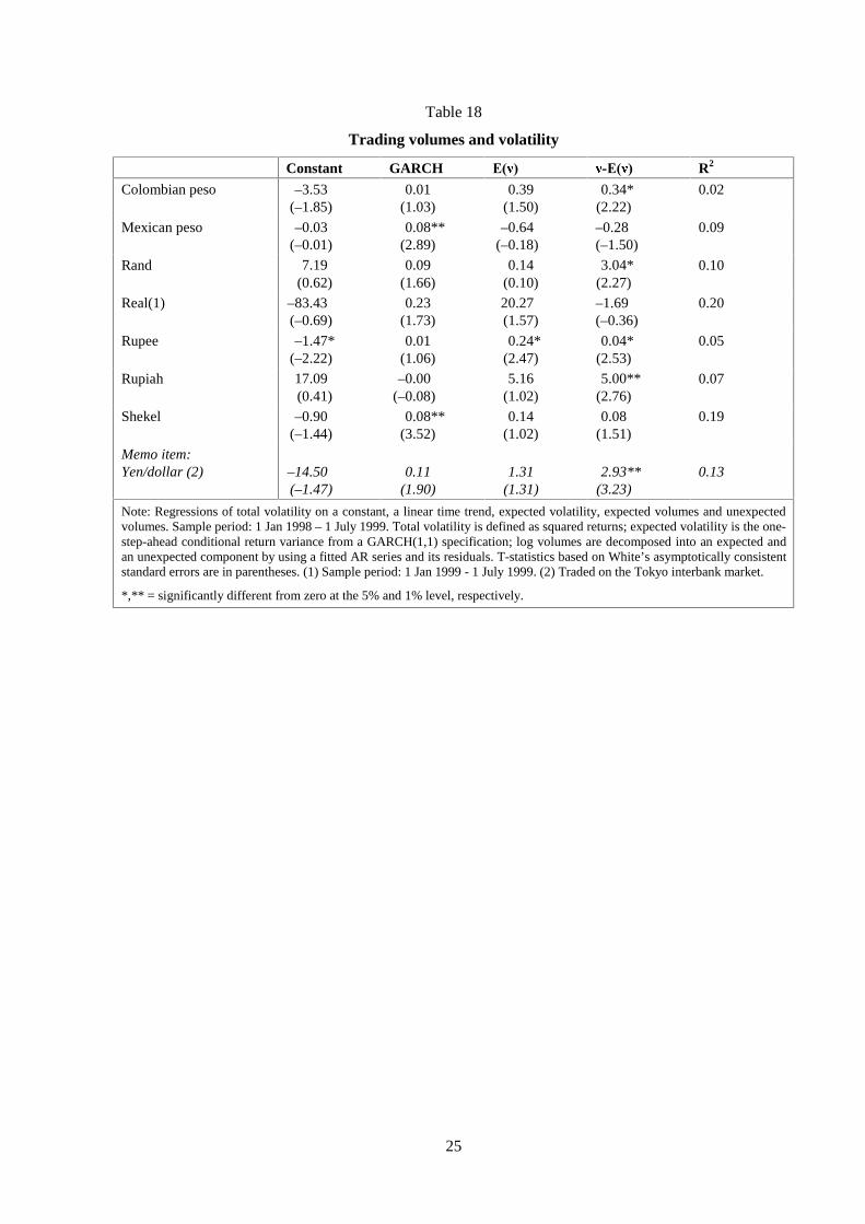
Table 18 shows the results for regressions that also include expected volatility, measured by the

GARCH forecast, among the explanatory variables. The coefficient on unexpected turnover remains

positive and statistically significant in most cases. This is in line with the results presented in Jorion

(1996). Again, the coefficient on unexpected trading volume is negative but not statistically significant

for the Mexican peso and the real. In these cases only, the GARCH volatility forecast is also

significant.

Overall, the results support the idea that the arrival of new public information drives the positive

correlation between volumes and volatility, as postulated by the mixture of distributions hypothesis.

Favourable evidence is found for four out of six exchange rates from emerging market countries and

for the Tokyo interbank yen/dollar market. These findings appear to be independent of market size. By

contrast, the mixture of distributions hypothesis appears not to hold for the Mexican peso/dollar and

real/dollar markets.

Since most emerging market currencies in the data set went through some periods of turbulence, it is

natural to test whether the correlation between volatility and volume is different in “normal” and

“stressful” times. The same argument may also hold for the dollar/yen rate, whose drastic change in

October 1998 was unprecedented by historical standards.

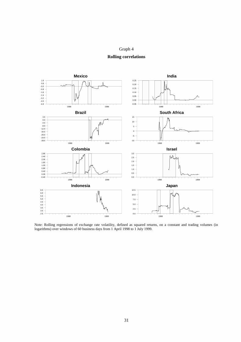
For each exchange rate, Graph 4 plots the coefficients of regressions of changes in volatility on a

constant and (the logarithm of) trading volumes estimated over rolling windows of three months. The

shaded areas indicate periods of turmoil. The charts suggest that the relationship between volatility

and trading volumes is indeed different in stressful and tranquil times. In the case of the real, the

Mexican peso and the rand, this relationship is strongly negative during periods of turbulence. This

suggests that the negative coefficient on trading volumes found in Tables 16-18 is driven by the

incidence of periods of stress.

One interpretation of this result is that the correlation between trading volumes and volatility is

positive during “normal” times, ie when volatility is relatively low. When volatility reaches very high

levels, this may induce traders to withdraw from the markets thereby leading to a negative correlation.

The mixture of distributions hypothesis may then hold in “normal” market conditions but be violated

during periods of market turmoil. Taking this argument one step further, one might posit that a

positive correlation between volume and volatility is an indication of liquid markets and a negative

correlation is a symptom of inadequate liquidity.

13

Trading volumes and bid-ask spreads

Graph 1 highlights that in foreign exchange markets in emerging market countries, bid-ask spreads

spiked during times in which volatility sharply increased and turnover fell. While spreads tended to

narrow shortly after these episodes, in some cases they remained wide for some time. Table 14 shows

that in foreign exchange markets in emerging market countries, spreads and volatility are positively

correlated. In most cases spreads and trading volumes are negatively correlated, a result that contrasts

with findings of the early literature.14 By contrast, the behaviour of spreads appears totally unrelated to

changes in volumes and volatility in the Tokyo yen/dollar interbank market, as indicated by

correlation coefficients close to zero.

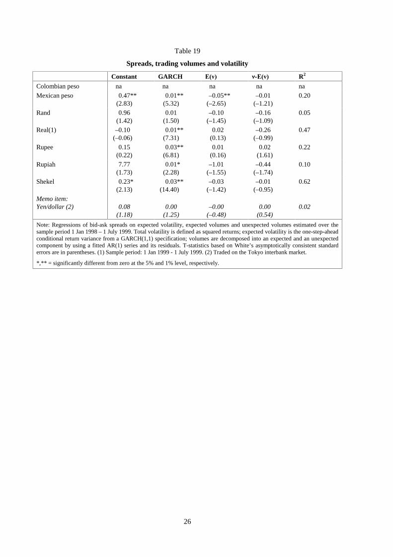
To test these assertions, I regressed bid-ask spreads on the GARCH variance forecasts and measures of

expected and unexpected trading volumes:

The results are presented in Table 19. Consistent with the findings of the literature, the coefficient on

the GARCH variance forecast is positive and statistically significant, suggesting that volatility

influences bid-ask spreads through its effect on inventory costs. However, in contrast to the

predictions of the theory, I do not find positive and significant coefficients on unexpected volumes.

The coefficients on expected volumes are also not statistically significant. One explanation is that the

sample period may be too short to allow for changes in these foreign exchange markets that lead to

more efficient trade processing and higher competition among market-makers.

5. Conclusions

This paper has tried to provide a contribution to the literature on the microstructure of foreign

exchange markets by investigating the empirical relationship between trading volumes, volatility and

bid-ask spreads. Until now, most of the research in this area has relied on data on futures markets,

since good data on turnover in foreign exchange markets were not easily available. One important

critique of this approach is that volumes in futures markets are not representative of total foreign

exchange market activity. This paper uses a new data set that includes daily data on trading volumes

for the dollar exchange rates of seven currencies from emerging market countries: the Indonesian

rupiah, the Indian rupee, the Mexican peso, the Brazilian real, the Colombian peso, the South African

rand and the Israeli shekel. To allow a comparison with other studies, it also looks at trading volumes

14 See eg Glassman (1987).

ttvttttt wEvvEhS εββββα ++−+++= −−+ 4)(131211 ][)()4(

14

from the Tokyo inter-dealer yen/dollar market. The data set covers the sample period 1 January 1998

to 30 June 1999.

An important result is that on average unexpected trading volumes and volatility are positively

correlated, suggesting that they both respond to the arrival of new information, as the mixture of

distributions hypothesis predicts. This is consistent with the findings of the literature that relies on

futures data. It suggests that the observation that futures markets are not representative is not

“damaging” (Dumas (1996)).

The markets for the Mexican peso and the real, however, provide important exceptions. In these two

cases, the relationship between unexpected volumes and volatility is negative but not statistically

significant. Moreover, for the Mexican peso data from foreign exchange markets and futures markets

yield opposite results, as unexpected futures volumes and volatility are positively correlated.

Evidence from rolling regressions suggests that for the real, the Mexican peso and the rand, the

relationship between volumes and volatility is strongly negative during periods of turbulence. This

indicates that the negative average coefficient on trading volumes is influenced by the incidence of

periods of stress. One possible interpretation is that the correlation between trading volumes and

volatility is positive during “normal” times but turns negative when volatility increases sharply,

implying that the mixture of distributions hypothesis holds under “normal” market conditions but not

during periods of stress.

I also find evidence of a positive correlation between volatility and spreads, as suggested by inventory

cost models. This result is also consistent with the findings of the literature. Finally, in contrast to

previous studies and to the mixture of distributions hypothesis, I do not find evidence of a significant

impact of unexpected trading volumes on spreads.

15

6. Tables and graphs

Table 1

Exchange rate regimes, 1998–99

Currency Exchange rate regime

Colombian peso Managed floating within an intervention band

Mexican peso Independent float

Rand Independent float

Real Managed floating within an adjustable band against the USdollar (mid-1995 to January 1999)

Rupee Independent float

Rupiah Free float (since the crisis in July 1997)

Shekel Managed with respect to a basket of currencies, withmargins of fluctuation of +/– 15%.1

1 The shekel has been fully convertible since May 1998.

Source: IMF Exchange Rate Arrangements and Restrictions, 1999.

Table 2

Summary statistics for exchange rate levels

Mean Std dev Min Max

Colombian peso 1486.19 116.28 1305.83 1752.18

Mexican peso 9.33 0.66 8.03 10.65

Rand 5.73 0.51 4.88 6.62

Real 1.36 0.30 1.12 2.19

Rupee 41.75 1.41 38.3 43.52

Rupiah 9614.66 2193.46 6000 16745

Shekel 3.89 0.24 3.55 4.37

Memo item:Yen/dollar 126.80 9.38 108.80 147.25

Note: Sample period: 1 Jan 1998 – 1 July 1999.

16

Table 3

Summary statistics for percentage changes of exchange rates

Mean Std devTest mean= 0

Skewness Kurtosis Min Max

Colombian peso 0.09 0.59 2.77(0.01)

2.42(0)

21.34(0)

–1.9 5.55

Mexican peso 0.04 0.76 1.07(0.28)

1.1(0)

6.15(0)

–2.94 4.49

Rand 0.06 1.05 1.14(0.25)

–1.33(0)

17.14(0)

–8.88 4.58

Real 0.13 1.4 1.78(0.08)

1.39(0)

28.15(0)

–10.77 11.41

Real(1.1 – 1.7.1999)

0.32 2.4 1.49(0.1)

0.58 7.59 –10.77 11.41

Rupee 0.03 0.29 1.81(0.07)

–0.24(0)

20.3(0)

–2.13 2.01

Rupiah 0.14 4.24 0.67(0.05)

1.05(0.06)

7.84(0)

–18.47 22.6

Shekel 0.04 0.5 1.5(0.14)

1.08(0)

7.4(0)

–2.25 2.87

Memo item:Yen/dollar –0.02 1.02 –0.29

(0.8)–1.00 5.57 –6.6 3.3

Note: Sample period: 1 Jan 1998 – 1 July 1999.

17

Table 4

Sample autocorrelation coefficients

1 2 5 10 20 60

Colombian peso

exchange rate 0.18 0.02 –0.04 0.04 –0.01 –0.05

volume –0.25 –0.06 –0.1 0.0 0.03 0.08

bid-ask spread na na na na na na

number of deals –0.24 –0.02 0.03 0.0 0.05 0.06

Mexican peso

exchange rate –0.03 0.02 0.02 0.09 0.06 0

volume –0.11 –0.03 0.01 0.01 –0.04 –0.01

bid-ask spread –0.21 –0.02 0.01 0.02 –0.02 –0.1

Rand

exchange rate –0.003 –0.04 0.21 0.09 –0.08 0.009

volume –0.18 –0.24 0.13 0.15 0.09 0.1

bid-ask spread –0.03 –0.004 –0.01 0.05 –0.01 –0.005

Real

exchange rate 0.15 0.16 –0.11 0.11 –0.01 –0.03

volume –0.18 0.01 –0.09 0.11 0.23 0.04

bid-ask spread –0.08 0.39 –0.05 0.005 –0.02 –0.02

Rupee

exchange rate 0.03 0.00 –0.02 0.023 0.01 –0.07

volume –0.00 –0.00 –0.00 –0.00 –0.00 –0.00

bid-ask spread –0.15 0.20 0.05 0.03 –0.02 –0.02

Rupiah

exchange rate 0.16 0.04 0 0.06 0.04 0.01

volume –0.4 0.12 0.09 –0.15 0.04 –0.01

bid-ask spread –0.01 –0.004 –0.004 –0.005 –0.004 –0.002

Shekel

exchange rate 0.12 0.2 –0.02 0.13 –0.05 0.03

volume –0.15 –0.01 0.22 0.08 0.02 0.18

bid-ask spread –0.38 0 –0.08 0.09 –0.04 0.04

Memo item:Yen/dollar

exchange rate 0.14 0.005 –0.02 0.03 0 0.05

volume –0.29 –0.06 0.21 0.15 0.06 0.02

bid-ask spread –0.37 –0.08 0.09 0.05 0.07 0.02

Note: Sample period: 1 Jan 1998 – 1 July 1999. All variables are expressed in percentage changes. Historicalvolatilities are computed with daily data over rolling windows of 20 business days. Bid-ask spreads are expressed as apercentage of the exchange rate.

18

Table 5

Summary statistics for one-month historical volatility

Mean Std dev Min Max

Colombian peso 7.94 4.66 1.64 21.97

Mexican peso 10.53 5.83 3.28 27.3

Rand 13.11 10.2 2.09 49.2

Real 10.98 18.24 0.56 76.15

Real (1.1.– 1.7.1999) 30.54 20.69 6.61 76.15

Rupee 3.73 2.75 0.69 10.66

Rupiah 55.47 38.85 8.35 175.26

Shekel 6.55 4.08 2.09 21.2

Memo item:Yen/dollar 15.33 5.51 7.76 32.46

Note: Sample period: 1 Jan 1998 – 1 July 1999. Historical volatilities are computed with daily data overrolling windows of 20 business days.

Table 6

Test for ARCH effects for percentage exchange rate changes

Lags 1 2 5 10

Colombian peso 0.00 0.03 0.44 11.77**

Mexican peso 16.25** 21.18** 83.95** 83.8**

Rand 8.1** 9.73** 59.16** 75.56**

Real 15.69** 15.35** 24.33** 40.3**

Rupee

Rupiah 16.82** 23.89** 67.72** 46.27**

Shekel 25.3** 71.2** 74.13** 75.6**

Note: The table reports results for Engle’s Lagrange multiplier-type test of time-varying heteroscedasticityregression residuals. The test statistics are reported for different lags (1 to 30). ** = the test statistic issignificant at the 1% level, suggesting the rejection of the null hypothesis of no ARCH effects.

19

Table 7

Regressions of volatility on a linear trend

Constant Time Dummy R2

Colombian peso –0.63*(–1.94)

0.001**(3.69)

–0.09(0.72)

0.01

Mexican peso 0.45(0.98)

0.00(0.30)

–0.06(–0.39)

0.01

Rand 2.74*(1.94)

–0.001(–1.34)

–0.54(–1.55)

0.01

Real(1) –11.95**(–4.14)

0.01**(4.02)

–1.02(–1.19)

0.02

Rupee 0.60**

(3.00)

–0.00**

(–2.76)

0.06

(0.89)

0.03

Rupiah 177.22**(4.94)

–0.16**(–4.81)

–4.38(–0.86)

0.11

Shekel 0.13(1.01)

0.0001(0.90)

0.03(0.41)

0.01

Memo item:Yen/dollar 1.18*

(1.93)–0.00

(–0.15)–0.31

(–1.42)0.01

Note: Regressions of volatility, computed as squared returns, on a linear time trend over thesample period 1 Jan 1998 – 1 July 1999. T-statistics are in parentheses. Trading volumes areexpressed in US$ millions. (1) Sample period: 1Jan 1999 - 1 July 1999.

*,** = significantly different from zero at the 5% and 1% level, respectively.

Table 8

Summary statistics for forex trading volumes

Mean Std dev Min Max

Colombian peso:Trading volume 165 72 16 362

Colombian peso:Number of trades per day 231 102.7 29 452

Mexican peso 8,827 2,281 635 15,812

Rand 9,535 2,410 3,432 21,568

Real 10,849 4,090 2,671 31,219

Real(1) 8,153 2,549 3,051 16,965

Rupee 3,478 1,351 1 8,211

Rupiah 1,072 250 611 1,871

Shekel 772 244 5 1,698

Memo item:Yen/dollar (2) 12,944 4,453 1,737 41,341

Note: Average daily turnover, in US$ millions. Sample period: 1 Jan 1998 – 30 June 1999. (1)Sample period: 1 Jan 1999 - 1 July 1999. (2) Traded on the Tokyo interbank market. In April1998, average daily global turnover for yen/dollar transactions amounted to US$ 267 billion.Total forex turnover in April 1998 was $ 1,500 billion.

20

Table 9

Summary statistics for exchange-traded volumes

Series Mean Std Dev Min Max

Real 16 35 0 277

Real (1) 224 484.27 0 4,164

Mexican peso 247 160 0 934

Mexican peso (1) 4,632 2,968.35 0 17,076

Rand 12 22 0 270

Rand (1) 142 275.35 0 3,361

Note: Notional values, in US$ millions. Sample period: January 1998 – June 1999. (1) Number of deals perday.

Table 10

Summary statistics for percentage changes of OTC trading volumes

Mean Std devTest mean= 0

Skewness Kurtosis Min Max

Colombian peso 7.5 45.16 3.17 (0) 2.95 20.17 –84.02 411.72

Colombian peso (2) 6.97 47.6 2.8 (0) 4.54 38.93 –81.77 505.71

Mexican peso 12.78 109.09 2.3 (0.02) 10.34 126.58 –93.04 1,542.37

Rand 2.65 26.24 1.6 (0.11) 1.24 4.4 –64.2 141.19

Real (1) 5.48 38.24 1.6 (0.12) 4.9 38.32 –73.49 318.59

Rupee

Rupiah 3.20 27.24 1.2 (0.25) 0.52 –0.13 –50.27 68.44

Shekel 4.05 30.70 4.6 (0) 7.73 85.99 –100.00 104.77

Memo item:Yen/dollar (3) 7.98 46.6 3.6 (0) 2.77 13.78 –78.06 346.88

Note: Sample period: January 1998 - June 1999. (1) Sample period 1 January 1999 – 1 July 1999. (2) Number of deals per day. (3)Traded on the Tokyo interbank market.

21

Table 11

Regressions of trading volumes on a linear trend

Constant Time Dummy R2

Colombian peso:Trading volume

315.64**(19.43)

–0.33**(–9.35)

–12.70(–1.70)

0.27

Colombian peso:Number of trades per day

506.72**(23.41)

–0.59**(–13.80)

–15.93(–1.64)

0.44

Mexican peso 11,345**(20.94)

–5.35**(–4.46)

–563.28**(–2.15)

0.07

Rand 12,992**(9.25)

–6.54**(–2.45)

–996.28**(–3.10)

0.07

Real (1) 28,454**(16.15)

–33.83**(–10.66)

–223.45(–0.47)

0.39

Rupee 6,786**

(11.79)

–3.41**

(–6.01)

126.94

(0.90)

0.08

Rupiah –296.27(–0.54)

2.37**(2.46)

–3.91(–0.07)

0.09

Shekel 127.48**(7.71)

–0.04(–1.25)

17.73*(2.04)

0.02

Memo item:Yen/dollar (2) 18,141**

(17.21)–9.74**

(–4.59)–1,993**

(–3.46)0.09

Note: Regressions of trading volumes on a linear time trend, over the sample period 1 Jan 1998 – 1 July 1999.T-statistics are in parentheses. Trading volumes are expressed in US$ millions. (1) Sample period: 1 Jan 1999– 1 July 1999. (2) Traded on the Tokyo interbank market. In April 1998, average daily global turnover foryen/dollar transactions amounted to US$ 267 billion.

*,** = significantly different from zero at the 5% and 1% level, respectively.

Table 12

Summary statistics for bid-ask spreads

Mean Std dev Min Max

Colombian peso na na na na

Mexican peso 0.12 0.08 0.02 0.94

Rand 0.20 0.63 0.01 12.27

Real 0.16 0.32 0.01 2.68

Real (1.1.-1.7.1999) 0.44 0.44 0.01 2.70

Rupee 0.37 0.23 0.00 2.36

Rupiah 2.11 1.49 0.14 8.70

Shekel 0.29 0.16 0.12 1.18

Memo item:Yen/dollar 0.05 0.02 0.02 0.09

Note: Sample period: 1 Jan 1998 – 1 July 1999. Bid-ask spreads are expressed as a percentage of the exchangerate. The data source is DRI.

22

Table 13

Summary statistics for percentage changes of bid-ask spreads

Mean Std devTest mean= 0

Skewness Kurtosis Min Max

Colombian peso na na na na na na na

Mexican peso 18.44 87.47 4.15 (0) 4.15 4.15 –84.9 853

Rand 34.4 401.6 1.68 (0.1) 18.55 357.1 –97.3 7763

Real 40.4 258.7 –92.3 3491

Real(1.1.– 1.7.1999)

69.57 417.68 1.89 (0.06) 6.71 46.76 –84.8 3,443.98

Rupee 0.03 0.29 1.81(0.07)

–0.24(0)

20.3(0)

–2.13 2.01

Rupiah 521.54 7,999 1.28 (0.2) 17.5 322.17 –1,056 15,0148

Shekel 4.07 28.8 2.78 (0) 1 2.31 –57.3 135.12

Memo item:Yen/dollar 12.9 58.4 4.3 (0) 1.39 2.38 –70.3 237.1

Note: Sample period: 1 Jan 1998 – 1 July 1999. Bid-ask spreads are expressed as a percentage of the exchange rate.

Table 14

Correlations

[U�volume

+xr,volume

-xr,volume

_ ;5_�volume

Volatility,volume

Hist vol,volume

[U�spread

Spread,volume

Spread,volatility

Colombian peso:Trading volume 0.08 0.14 0.05 0.08 0.09 0.01 na na naColombian peso:Number of trades per day

0.13 0.15 0.03 0.13 na na na

Mexican peso 0.06 –0.10 0.17 –0.11 –0.10 –0.28 0.26 –0.15 0.64

Rand 0.16 0.27 –0.11 0.20 0.14 –0.08 0.15 –0.05 0.14

Real –0.17 –0.42 0.26 –0.37 –0.21 –0.57 0.31 –0.47 0.56

Real(1.1.– 1.7.1999)

–0.25 –0.31 –0.02 –0.05 –0.01 –0.28 0.32 –0.30 0.35

Rupee 0.10 0.37 –0.35 0.38 0.28 0.40 0.13 0.38 0.38

Rupiah –0.09 0.17 –0.30 0.21 0.10 –0.02 –0.05 –0.20 0.30

Shekel 0.04 0.30 –0.27 0.28 0.25 0.09 0.17 0.16 0.43

Memo item:

Yen/dollar –0.16 0.47 –0.45 0.45 0.40 0.15 –0.09 0.08 0.08

Note: Correlation coefficients are computed for the period 1 Jan 1998 – 1 July 1999. Exchange rate changes are percentage changes;volumes are expressed in logarithms; bid-ask spreads are expressed as a fraction of the spot rate; volatility is computed as squaredreturns; historical volatility is computed as standard deviations of daily percentage exchange rate changes over rolling windows of 20business days.

23

Table 15

Correlations for exchange-traded volumes

[U�volume

+xr,volume

-xr,volume

_ ;5_�volume

Volatility,volume

Hist vol,volume

Spread,volume

Mexican peso 0.09 0.28 –0.11 0.22 0.16 0.04 0.07

Note: Correlation coefficients are computed for the period 1 Jan 1998 – 1 July 1999. Volumes refer to notional amounts inUS$ millions. The other variables are defined as in Table 14.

Table 16

Volatility and trading volume: unconditional regressions

Constant Time trend Volume R2

Colombian peso –3.86**(–2.88)

0.0022**(4.16)

0.41*(2.14)

0.02

Colombian peso (1) –1.62(–0.83)

0.0008(0.42)

0.23*(2.46)

0.04

Mexican peso 2.89(1.54)

0.0002(0.44)

–0.28(–1.58)

0.00

Rand –2.11(–0.36)

–0.02**(–2.75)

2.17*(2.30)

0.06

Real(2) 121.19(1.75)

–0.02(–1.05)

–10.80*(–1.92)

0.07

Rupee 0.21(1.24)

–0.001**(–2.65)

0.05**(2.87)

0.04

Rupiah 20.10(0.76)

–0.05(–1.80)

5.01**(3.49)

0.07

Shekel –1.06*(–2.68)

0.0002*(2.06)

0.23**(2.75)

0.04

Memo item:Yen/dollar (3) –32.18**

(–2.98)0.0023*

(2.45)3.26**

(3.03)0.12

Note: Regressions of exchange rate volatility, defined as squared returns, on a constant, a linear time trend andtrading volumes (in logarithms) over the sample period 1 Jan 1998 – 1 July 1999. T-statistics based on White’sasymptotically consistent standard errors are in parentheses. Coefficients on trading volumes are multiplied by100. (1) Number of deals per day. (2) Sample period: 1 Jan 1999 - 1 July 1999. (3) Traded on the Tokyointerbank market.

*,** = significantly different from zero at the 5% and 1% level, respectively.

24

Table 17

Trading volumes and volatility

Constant (� � �(� � R2

Colombian peso –4.04–(2.47)

0.44(1.91)

0.34*(2.27)

0.02

Mexican peso 3.09(0.82)

–0.28(–0.78)

–0.30(–1.50)

0.00

Rand 7.50(0.66)

1.31(0.98)

3.08*(2.47)

0.07

Real(1) 69.93(1.04)

14.28(1.26)

–2.83(–0.62)

0.15

Rupee –1.70**(–2.74)

0.29**(3.16)

0.04**(2.91)

0.05

Rupiah 17.41(0.41)

5.32(1.19)

4.97**(2.96)

0.07

Shekel –2.63**(–2.87)

0.56**(2.91)

0.18**(2.65)

0.05

Memo item:Yen/dollar (2) –27.27*

(–2.04)2.78*

(2.03)3.20**

(3.06)0.11

Note: Regressions of total volatility on a constant, a linear time trend, expected volumes and unexpected volumes.Sample period: 1 Jan 1998 – 1 July 1999. Total volatility is defined as squared returns; log volumes aredecomposed into an expected and an unexpected component by using a fitted AR series and its residuals.T-statistics based on White’s asymptotically consistent standard errors are in parentheses. (1) Sample period: 1 Jan1999 - 1 July 1999. (2) Traded on the Tokyo interbank market.

*,** = significantly different from zero at the 5% and 1% level, respectively.

25

Table 18

Trading volumes and volatility

Constant GARCH (� � �(� � R2

Colombian peso –3.53(–1.85)

0.01(1.03)

0.39(1.50)

0.34*(2.22)

0.02

Mexican peso –0.03(–0.01)

0.08**(2.89)

–0.64(–0.18)

–0.28(–1.50)

0.09

Rand 7.19(0.62)

0.09(1.66)

0.14(0.10)

3.04*(2.27)

0.10

Real(1) –83.43(–0.69)

0.23(1.73)

20.27(1.57)

–1.69(–0.36)

0.20

Rupee –1.47*(–2.22)

0.01(1.06)

0.24*(2.47)

0.04*(2.53)

0.05

Rupiah 17.09(0.41)

–0.00(–0.08)

5.16(1.02)

5.00**(2.76)

0.07

Shekel –0.90(–1.44)

0.08**(3.52)

0.14(1.02)

0.08(1.51)

0.19

Memo item:Yen/dollar (2) –14.50

(–1.47)0.11

(1.90)1.31

(1.31)2.93**

(3.23)0.13

Note: Regressions of total volatility on a constant, a linear time trend, expected volatility, expected volumes and unexpectedvolumes. Sample period: 1 Jan 1998 – 1 July 1999. Total volatility is defined as squared returns; expected volatility is the one-step-ahead conditional return variance from a GARCH(1,1) specification; log volumes are decomposed into an expected andan unexpected component by using a fitted AR series and its residuals. T-statistics based on White’s asymptotically consistentstandard errors are in parentheses. (1) Sample period: 1 Jan 1999 - 1 July 1999. (2) Traded on the Tokyo interbank market.

*,** = significantly different from zero at the 5% and 1% level, respectively.

26

Table 19

Spreads, trading volumes and volatility

Constant GARCH (� � �(� � R2

Colombian peso na na na na na

Mexican peso 0.47**(2.83)

0.01**(5.32)

–0.05**(–2.65)

–0.01(–1.21)

0.20

Rand 0.96(1.42)

0.01(1.50)

–0.10(–1.45)

–0.16(–1.09)

0.05

Real(1) –0.10(–0.06)

0.01**(7.31)

0.02(0.13)

–0.26(–0.99)

0.47

Rupee 0.15(0.22)

0.03**(6.81)

0.01(0.16)

0.02(1.61)

0.22

Rupiah 7.77(1.73)

0.01*(2.28)

–1.01(–1.55)

–0.44(–1.74)

0.10

Shekel 0.23*(2.13)

0.03**(14.40)

–0.03(–1.42)

–0.01(–0.95)

0.62

Memo item:Yen/dollar (2) 0.08

(1.18)0.00

(1.25)–0.00

(–0.48)0.00

(0.54)0.02

Note: Regressions of bid-ask spreads on expected volatility, expected volumes and unexpected volumes estimated over thesample period 1 Jan 1998 – 1 July 1999. Total volatility is defined as squared returns; expected volatility is the one-step-aheadconditional return variance from a GARCH(1,1) specification; volumes are decomposed into an expected and an unexpectedcomponent by using a fitted AR(1) series and its residuals. T-statistics based on White’s asymptotically consistent standarderrors are in parentheses. (1) Sample period: 1 Jan 1999 - 1 July 1999. (2) Traded on the Tokyo interbank market.

*,** = significantly different from zero at the 5% and 1% level, respectively.

27

Graph 1

Trading volumes, volatility and spreads

BRAZIL COLOMBIA MEXICO JAPAN

* Expressed in million US$. ** 1-month historical volatility. *** As a percentage of the mid quote.

1.0

1.4

1.8

2.2

2.6

1.Ja

n .9 8

1.M

a r. 9

8

1 .M

a y. 9

8

1 .Ju

l. 98

1 .S

ep.9

8

1 .N

ov.9

8

1.Ja

n.99

1.M

ar.9

9

1.M

a y.9

9

0

10000

20000

30000

40000Spot rate (lhs)Volume* (rhs)

0

20

40

60

80

1.Ja

n.98

1.M

a r.9

8

1.M

ay.9

8

1 .Ju

l. 98

1 .S

ep.9

8

1 .N

ov.9

8

1.J a

n.9 9

1 .M

a r.9

9

1.M

a y.9

9

0

10000

20000

30000

40000Volatility** (lhs)

Volume* (rhs)

0

20

40

60

80

1.Ja

n.9 8

1 .M

ar.9

8

1 .M

ay.9

8

1.Ju

l.98

1 .S

ep.9

8

1 .N

ov.9

8

1 .J a

n .99

1.M

a r.9

9

1.M

a y.9

9

0.00

1.00

2.00

3.00

4.00Volatility** (lhs)

Bid-ask spread***(rhs)

1300

1400

1500

1600

1700

1800

1.Ja

n.98

1.M

ar.9

8

1 .M

a y. 9

8

1.Ju

l.98

1 .S

ep.9

8

1.N

o v.9

8

1 .Ja

n .9 9

1 .M

a r.9

9

1.M

ay.9

9

0

100

200

300

400

500

0

5

10

15

20

25

1.Ja

n.9 8

1 .M

a r.9

8

1 .M

a y. 9

8

1.J u

l.98

1.S

e p. 9

8

1.N

o v. 9

8

1.Ja

n.99

1.M

a r.9

9

1.M

a y. 9

9

0

100

200

300

400

500

0

5

10

15

20

25

1.Ja

n .98

1 .M

ar.9

8

1.M

a y. 9

8

1.Ju

l.98

1 .S

ep.9

8

1.N

o v. 9

8

1.Ja

n.99

1 .M

ar.9

9

1 .M

a y. 9

9

8

9

10

11

1.Ja

n .9 8

1 .M

a r. 9

8

1 .M

a y. 9

8

1 .J u

l .98

1 .S

ep.9

8

1 .N

ov.9

8

1.Ja

n.99

1 .M

a r. 9

9

1 .M

a y. 9

9

0

6000

12000

18000

0

10

20

30

1.Ja

n .9 8

1 .M

a r.9

8

1.M

ay.9

8

1 .J u

l. 98

1 .S

ep.9

8

1.N

o v. 9

8

1 .J a

n .9 9

1 .M

ar.9

9

1.M

a y. 9

9

0

6000

12000

18000

0

10

20

30

1.Ja

n .9 8

1.M

ar. 9

8

1.M

a y. 9

8

1 .J u

l .98

1.S

e p.9

8

1.N

o v. 9

8

1.J a

n .9 9

1.M

ar.9

9

1.M

ay.9

9

0.00

0.40

0.80

1.20

100

110

120

130

140

150

1.Ja

n .9 8

1 .M

ar.9

81 .

Ma y

. 98

1 .J u

l .98

1 .S

e p. 9

81.

No v

.98

1.Ja

n.99

1.M

a r. 9

91.

May

.99

0

10000

20000

30000

40000

50000

0

10

20

30

40

1.Ja

n.9 8

1 .M

ar.9

8

1 .M

a y.9

8

1 .J u

l .98

1 .S

ep.9

8

1 .N

o v.9

8

1 .J a

n .9 9

1 .M

ar.9

9

1 .M

ay.9

9

0

12000

24000

36000

48000

0

10

20

30

40

1.Ja

n.98

1.M

a r. 9

8

1 .M

ay.9

8

1 .J u

l .98

1.S

e p. 9

8

1.N

ov.9

8

1 .J a

n .9 9

1 .M

a r.9

9

1.M

a y.9

9

0.00

0.10

0.20

0.30

0.40

28

Graph 1 (continued)

Trading volumes, volatility and spreads

INDIA INDONESIA ISRAEL SOUTH AFRICA

* Expressed in million US$. ** 1-month historical volatility. *** As a percentage of the mid quote.

35

39

43

47

1.Ja

n .9 8

1.M

ar. 9

8

1 .M

ay.9

8

1.J u

l.98

1.S

e p.9

8

1 .N

ov.9

8

1.J a

n.99

1 .M

a r.9

9

1.M

ay.9

90

4000

8000

12000Spot rate (lhs)

Volume* (rhs)

0

4

8

12

1.Ja

n.9 8

1 .M

ar.9

8

1 .M

a y. 9

8

1.Ju

l.98

1 .S

ep.9

8

1 .N

o v. 9

8

1.Ja

n.99

1 .M

a r.9

9

1.M

ay.9

9

0

4000

8000

12000Volatility** (lhs)

Volume* (rhs)

0

4

8

12

1.Ja

n.9 8

1 .M

ar.9

8

1 .M

ay.9

8

1 .J u

l. 98

1 .S

ep.9

8

1 .N

ov.9

8

1 .J a

n .9 9

1.M

a r. 9

9

1.M

a y.9

9

0.0

1.0

2.0

3.0Volatility** (lhs)

Bid-ask spread*** (rhs)

0

40

80

120

160

200

1.Ja

n .9 8

1.M

a r. 9

8

1 .M

ay.9

8

1 .J u

l .98

1 .S

e p. 9

8

1.N

o v.9

8

1 .J a

n .9 9

1.M

a r. 9

9

1 .M

ay.9

9

0

400

800

1200

1600

2000

0

40

80

120

160

200

1.Ja

n.98

1 .M

a r.9

8

1 .M

a y. 9

8

1 .J u

l.98

1 .S

e p.9

8

1.N

o v. 9

8

1.J a

n.9 9

1 .M

ar.9

9

1 .M

ay.9

9

0

2

4

6

8

10

3.2

3.6

4.0

4.4

1.Ja

n .9 8

1 .M

ar.9

8

1.M

a y. 9

8

1 .Ju

l.98

1 .S

ep.9

8

1.N

o v. 9

8

1 .Ja

n .9 9

1.M

ar. 9

9

1 .M

a y.9

9

0

600

1200

1800

0

10

20

30

1.Ja

n.98

1 .M

ar.9

8

1 .M

a y.9

8

1 .J u

l. 98

1 .S

ep.9

8

1 .N

ov.9

8

1 .Ja

n .99

1 .M

a r.9

9

1 .M

a y.9

9

0

600

1200

1800

0

10

20

30

1.Ja

n .9 8

1.M

a r. 9

8

1 .M

a y. 9

8

1 .J u

l .98

1 .S

ep.9

8

1.N

ov.9

8

1.Ja

n.99

1 .M

ar.9

9

1.M

ay.9

9

0.0

0.4

0.8

1.2

4.5

5.0

5.5

6.0

6.5

7.0

1.Ja

n.98

1.M

ar. 9

8

1 .M

a y. 9

8

1 .Ju

l. 98

1.S

e p. 9

8

1 .N

o v.9

8

1 .Ja

n .9 9

1 .M

ar.9

9

1.M

a y.9

9

0

6000

12000

18000

24000

30000

0

10

20

30

40

50

1.Ja

n .9 8

1 .M

ar.9

8

1 .M

a y. 9

8

1.Ju

l.98

1 .S

ep.9

8

1 .N

o v. 9

8

1 .Ja

n .99

1.M

a r. 9

9

1 .M

ay.9

9

0

6000

12000

18000

24000

30000

0

10

20

30

40

50

1.Ja

n.98

1 .M

a r. 9

8

1.M

ay.9

8

1 .J u

l .98

1 .S

e p. 9

8

1 .N

ov.9

8

1 .J a

n .9 9

1 .M

ar.9

9

1 .M

a y. 9

9

0.00

4.00

8.00

12.00

16.00

20.00

5000

8000

11000

14000

17000

1.Ja

n.98

1.M

a r. 9

8

1.M

ay.9

8

1 .J u

l .98

1.S

e p. 9

8

1 .N

ov.9

8

1 .J a

n .9 9

1 .M

ar.9

9

1 .M

a y. 9

9

0

500

1000

1500

2000

29

Graph 2

Trading volumes and volatility in selected emerging markets

Note: Trading volumes refer to local turnover in the domestic currency, per trading day in the month shown (in millions ofUS dollars). In the case of Mexico and Brazil, turnover includes other currencies. Volatility is computed as the one-monthannualised standard deviation of percentage changes in the exchange rate against the US dollar.

Korean won

0

1000

2000

3000

4000

5000

6000

7000

8000

9000

1995:01 1996:01 1997:01 1998:01 1999:01 2000:01

020406080100120140160180200

Brazilian real

0

2000

4000

6000

8000

10000

12000

1995:01 1996:01 1997:01 1998:01 1999:01 2000:01

0

10

20

30

40

50

60

70

80

Colombian peso

0

100

200

300

1995:01 1996:01 1997:01 1998:01 1999:01 2000:01

0.00

5.00

10.00

15.00

20.00

25.00

30.00

South African rand

0

1000

2000

3000

4000

5000

6000

7000

8000

9000

1995:01 1996:01 1997:01 1998:01 1999:01 2000:01

0

10

20

30

40

50

60

70

80

Indonesian rupiah

0

1000

2000

3000

4000

5000

6000

7000

8000

9000

1995:01 1996:01 1997:01 1998:01 1999:01 2000:01

020406080100120140160180200

Indian rupee

0

1000

2000

3000

4000

5000

1995:01 1996:01 1997:01 1998:01 1999:01 2000:01

0

10

20

30

40

50

60

70

80

Mexican peso

0

2000

4000

6000

8000

10000

12000

1995:01 1996:01 1997:01 1998:01 1999:01 2000:010

10

20

30

40

50

60

70

80

Israeli shekel

0

200

400

600

800

1000

1200

1995:01 1996:01 1997:01 1998:01 1999:01 2000:010.00

5.00

10.00

15.00

20.00

25.00

30.00

30

Graph 3

OTC and exchange-traded foreign exchange market turnover

Note: OTC turnover is defined as in Graph 1. Exchange-traded turnover refers to notional values of futures contractstransacted on the Chicago Mercantile Exchange.

Brazilian real

0

5000

10000

15000

20000

25000

30000

35000

01.0

1 .1 9

9 8

01.0

3.19

9 8

0 1. 0

5 .1 9

9 8

0 1. 0

7 .1 9

9 8

0 1. 0

9 .1 9

9 8

0 1. 1

1 .1 9

98

0 1.0

1.19

99

0 1.0

3 .1 9

99

0 1.0

5.19

99

0

50

100

150

200

250

300

350OTC (lhs)

Exchange traded (rhs)

Mexican peso

0

4000

8000

12000

16000

20000

01.0

1 .1 9

9 8

0 1. 0

3 .1 9

9 8

0 1.0

5.1 9

98

01.0

7.19

9 8

01.0

9 .19

9 8

0 1. 1

1 .1 9

9 8

0 1.0

1.1 9

99

0 1.0

3.1 9

99

01.0

5.19

9 9

0

200

400

600

800

1000

South African rand

0

4000

8000

12000

16000

20000

01.0

1.19

98

0 1.0

3 .1 9

98

0 1.0

5.19

98

01.0

7.19

9 8

0 1.0

9.19

98

01.1

1.19

9 8

01.0

1 .19

9 9

01.0

3.19

99

01.0

5.19

9 9

0

20

40

60

80

100

31

Graph 4

Rolling correlations

Note: Rolling regressions of exchange rate volatility, defined as squared returns, on a constant and trading volumes (inlogarithms) over windows of 60 business days from 1 April 1998 to 1 July 1999.

Mexico

1998 1999-4.8

-4.0

-3.2

-2.4

-1.6

-0.8

-0.0

0.8

1.6

Brazil

1998 1999-28.0

-24.0

-20.0

-16.0

-12.0

-8.0

-4.0

0.0

4.0

Colombia

1998 1999-0.40

0.00

0.40

0.80

1.20

1.60

2.00

2.40

2.80

Indonesia

1998 19992.5

3.0

3.5

4.0

4.5

5.0

5.5

6.0

6.5

India

1998 1999-0.05

0.00

0.05

0.10

0.15

0.20

0.25

South Africa

1998 1999-10

-5

0

5

10

15

Israel

1998 19990.0

0.5

1.0

1.5

2.0

2.5

3.0

Japan

1998 19990.0

2.5

5.0

7.5

10.0

12.5

32

References

Batten and Bhar (1993): “Volume and volatility in yen futures markets: within and across threedifferent exchanges”. Macquarie University Working Paper.

Bessembinder, Hendrik (1994): “Bid-ask spreads in the interbank foreign exchange markets”. JournalFinancial Economics, 35(3), pp. 317-348.

BIS (1997): 67th Annual report.

BIS (1998): International banking and financial market developments. November.

BIS (1999a): “Market liquidity: research findings and selected policy implications”. Report for theCGFS.

BIS (1999b): Central bank survey of foreign exchange and derivatives market activity.

Bollerslev, Tim and I Domowitz (1993): “Trading patterns and prices in the interbank foreignexchange market”. Journal of Finance, 48, pp. 1421-43.

Bollerslev, Tim and Michael Melvin (1994): “Bid-ask spreads and volatility in the foreign exchangemarket: an empirical analysis”. Journal of International Economics, Vol. 36, pp. 355-372.

Cheung, Yin-Wong and Menzie Chinn (1999):“Traders, market microstructure and exchange ratedynamics”. NBER Working Paper 7416, November.

Clark P K (1973): “A subordinated stochastic process model with finite variance for speculativeprices”. Econometrica, Vol. 41, pp. 135-155.

Copeland (1976): “A model of asset trading under the assumption of sequential information arrival”.Journal of Finance, Vol. 31, pp. 1149-1168.

Copeland (1977): “A probability model of asset trading”. Journal of Financial and QuantitativeAnalysis, Vol. 12, pp. 563-578.

Cornell B (1978): “Determinants of the bid-ask spread on forward foreign exchange contracts underfloating exchange rates”. Journal of International Business Studies, Vol. 9, pp. 33-41.

Cornell B (1981): “The relationship between volume and price variability in futures markets”. TheJournal of Futures Markets, Vol. 1, pp. 303-316.

Dumas, Bernard (1996): “Comment on Jorion”, in Frankel, Galli and Giovannini The Microstructureof Foreign Exchange Markets. University of Chicago Press, Chicago, pp. 37-40.

Glassman, Debra (1987): “Exchange rate risk and transaction costs: evidence from bid-ask spreads”.Journal of International Money and Finance, Vol. 6(4), pp. 479-490.

Goodhart, C and L Figliuoli (1991): “Every minute counts in financial markets”. Journal ofInternational Money and Finance, Vol. 10, pp. 23-52.

Goodhart, C, T Ito and R Payne (1996): “One day in June 1993: A study of the working of the Reuters2000-2 electronic foreign exchange trading system”, in Frankel, Galli and Giovannini TheMicrostructure of Foreign Exchange Markets, University of Chicago Press, Chicago, pp. 107-179.

Grammatikos T and A Saunders (1986): “Futures price variability: a test of maturity and volumeeffects”. Journal of Business, Vol. 59, pp. 319-330.

Harris, L (1986): “Cross-security tests of the mixture of distributions hypothesis”. Journal ofFinancial and Quantitative Analysis, Vol. 21, pp. 39-46.

Hartmann, Philipp (1998a): “Do Reuters spreads reflect currencies’ differences in global tradingactivity” in Currency Composition and Foreign Exchange Markets. Cambridge University Press, pp.132-162.

33

Hartmann, Philipp (1998b): “Trading volumes and transaction costs: from the short run to the longrun” in Currency Composition and Foreign Exchange Markets. Cambridge University Press.

Hartmann, Philipp (1999): “Trading volumes and transaction costs in the foreign exchange market”.Journal of Banking and Finance, Vol. 23, pp. 801-824.

Jorion, Philippe (1996): “Risk and turnover in the foreign exchange market”, in Frankel, Galli andGiovannini The Microstructure of Foreign Exchange Markets, University of Chicago Press, Chicago,pp. 19-36.

Karpoff, Jonathan (1987): “The relation between price changes and trading volume: a survey”. Journalof Financial and Quantitative Analysis, Vol. 22(1), pp. 109-126.

Lyons, Richard (1995): “Test of microstructural hypotheses in the foreign exchange market”. Journalof Financial Economics, Vol. 39, pp. 321-351.

Lyons, Richard (2000): The microstructure approach to exchange rates. MIT Press, forthcoming.

Melvin, Michael and Xixi Yin (2000): “Public information arrival, exchange rate volatility and quotefrequency”. The Economic Journal.

Richardson, G, S E Sefcik and R Thomson (1987): “A test of dividend irrelevance using volumereaction to a change in dividend policy”. Journal of Financial Economics, Vol. 17, pp. 313-333.

Shang-Jin, Wei (1994): “Anticipations of foreign exchange volatility and bid-ask spreads”. NBERWorking Paper No. 4737.

Tauchen, G and M Pitts (1983): “The price-variability volume relationship on speculative markets”.Econometrica, Vol. 51 (March), pp. 485-505.

Recent BIS Working Papers

No Title Author

77October 1999

Perceived central bank intervention and marketexpectations: an empirical study of the yen/dollarexchange rate, 1993-96

Gabriele Galati andWilliam Melick

78October 1999

Banking and commerce: a liquidity approach Joseph G Haubrichand João A C Santos

79November 1999

Pass-through of exchange rates and import prices todomestic inflation in some industrialised economies

Jonathan McCarthy

80November 1999

A note on alternative measures of real bond rates Palle S Andersen

81November 1999

Interbank interest rates and the risk premium Henri Pagès

82November 1999

Sacrifice ratios and the conduct of monetary policy inconditions of low inflation

Palle S Andersen andWilliam L Wascher

83January 2000

Switching from single to multiple bank lendingrelationships: determinants and implications

Luísa A Farinha andJoão A C Santos

84January 2000

What have we learned from recent financial crises andpolicy responses?

William R White

85January 2000

A defence of the expectations theory as a model of USlong-term interest rates

Gregory D Sutton

86March 2000

Information, liquidity and risk in the internationalinterbank market: implicit guarantees and private creditmarket failure

Henri Bernard andJoseph Bisignano

87May 2000

Monetary policy in an estimated optimisation-basedmodel with sticky prices and wages

Jeffery D Amato andThomas Laubach

88June 2000

Evidence on the response of US banks to changes incapital requirements

Craig Furfine

89August 2000

Forecast-based monetary policy Jeffery D Amato andThomas Laubach

90September 2000

Bank capital regulation in contemporary bankingtheory: a review of the literature

João A C Santos

91October 2000

Measuring potential vulnerabilities in emerging marketeconomies

John Hawkins andMarc Klau

92October 2000

Recent initiatives to improve the regulation andsupervision of private capital flows

William R White

ISSN 1020-0959