Trading quasi-emission permits

by

02-001 January 2002

Juan-Pablo Montero

WP

Trading quasi-emission permits

Juan-Pablo Montero¤

Catholic University of Chile and MIT

January 31, 2002

Abstract

I study the design of environmental policies for a regulator that has incomplete informa-

tion on …rms’ emissions and costs of production and abatement (e.g., air pollution in cities

with numerous small polluting sources). Because of incomplete information on emissions,

there is no policy that can implement the …rst-best. Since the regulator can observe …rms’

abatement technologies, however, it is possible to design a quasi-emissions trading program

based on this information and show that it can provide higher welfare than command-and-

control regulation such as technology or emission standards. I then empirically examine this

claim using evidence from a particulate quasi-emissions trading program in Santiago, Chile.

¤<jpmonter@mit.edu> Professor of Economics at the Department of Economics of the Catholic University ofChile (PUC), Research Associate at the MIT Center for Energy and Environmental Policy Research (CEEPR),and Visiting Professor of Applied Economics at the MIT Sloan School of Management. I am grateful to LuisCifuentes, Denny Ellerman, Shreekant Gupta, José Miguel Sánchez and seminar participants at MIT and PUCfor comments and discussions; Rodrigo San Martín for research assistance; and the Chile’s National Commisionfor the Environment and CEEPR for …nancial support.

1

1 Introduction

In recent years, environmental policy makers are paying more attention to environmental mar-

kets (i.e., emissions trading programs) as an alternative to the traditional command-and-control

(CAC) approach of setting emission and technology standards. A notable example is the 1990

U.S. acid rain program that implemented a nationwide market for electric utilities’ sulfur diox-

ide (SO2) emissions (Schmalensee et al., 1998; Ellerman et al., 2000). In order to have a precise

estimate of the SO2 emissions that are actually going to the atmosphere, the acid rain program

requires each a¤ected electric utility unit to install costly equipment that can continuously

monitor emissions.1

This and other market experiences suggest that conventional emissions trading programs

are likely to be implemented in those cases where emissions can be closely monitored, which

almost exclusively occurs in large stationary sources like electric power plants and re…neries.

, it is not surprising that, among other reasons, environmental authorities continue relying

on CAC instruments to regulate emissions from smaller sources because compliance with such

instruments only requires the authority to ensure that the regulated source has installed the

required abatement technology or that its emissions per unit of output are equal or lower than

a certain emissions rate standard.2 In addition, some regulators view that a trading program

where emissions cannot be closely observed is likely to result in higher emissions than under

an alternative CAC regulation because the former provides …rms with more incentives to alter

1Another example with similar monitoring requirements is the Southern California RECLAIM program thatimplemented separated markets for nitrogen oxide (NOx) and SO2 emissions from power plants, re…neries andother large stationary sources. This program did not include a market for volatile organic compounds (VOC) inlarge part because of the di¢culties with monitoring actual emissions from smaller and heterogeneous sources(Harrison, 1999).

2Note that there are some credit-based trading programs aimed at curbing air pollution in urban areas workingin the US (Tietenberg, 1985). New sources (or expansion of existing ones) must acquire emission credits to covertheir emissions through, for example, shutting down existing plants or scrapping old vehicles. Although theseprograms have the merit of involving small sources, they are very limited in scope in the sense that they areembedded within an existing CAC regulation and are particularly designed to prevent further deterioration ofair quality from the entry of new sources.

2

their output and hence their actual emissions.3

Thus, it appears that environmental markets are not suitable for e¤ectively reducing air

pollution in cities such as Santiago-Chile or Mexico City where emissions come from many

small (stationary and mobile) sources rather than a few large stationary sources. For example,

it would be prohibitively costly to require operators of central heating systems in residential

or commercial buildings to install continuous emission monitoring equipment. Through annual

inspections, however, the regulator could monitor boilers’ size, combustion technology, fuel type

and emissions rate as he would precisely do under CAC regulation. But since the regulator does

not observe the total number of hours boilers are operated during the year, he would certainly

have imperfect estimates of boilers’ actual emissions.

Rather than disregard environmental markets as a policy tool, I think the challenge faced by

policy makers in cities su¤ering similar air quality problems is when and how to implement these

markets using monitoring procedures that are similar to those under CAC regulation. While

the literature provides little guidance on how to approach this challenge,4 it is interesting to

observe that despite its incomplete information on each source’s actual emissions, Santiago-

Chile’s environmental agency has already implemented a market to control total suspended

particulate (TSP) emissions from a group of about 600 stationary sources (Montero et al., 2002).

Based on estimates from annual inspection for technology parameters such as source’s size and

fuel type, Santiago’s environmental regulator approximates each source’s actual emissions by

the maximum amount of emissions that the source could potentially emit in a given year.5

3Several conversations during 2000 and 2001 with some regulators at Chile’s National Commission for theEnvironment.

4 In his survey, Lewis (1996) brie‡y explains the implications of imperfect monitoring on instrument design.Lewis and Sappington (1992) study a similar situation in which a regulator cannot observe the quality of service(e.g., energy conservation) o¤ered by a public utility. In addition, Fullerton and West (forthcoming) discuss theuse of taxes on cars and on gasoline as an alternative to an unavailable tax on emissions.

5The authority incorrectly assumed that by using the source’s maximum emissions as a proxy it would preventperverse incentives that could result in higher emissions. As we shall see, the choice of proxy is an arbitrarymatter because the number of permits being allocated can always be adjusted accordingly with no e¢ciencye¤ects.

3

I believe that a close (theoretical and empirical) examination of this quasi-emissions trading

program represents a unique case study of issues of instrument choice and design that can arise

in the practical implementation of environmental markets in which regulators face important

information asymmetries and have a limited number of policy instruments (e.g., cannot make

transfers from or to …rms).

Since a¤ected sources under Santiago’s quasi-emissions trading program (hereafter, the TSP

program) were responsible for only 4.8% of TSP emissions in Santiago in 2000 (Cifuentes and

Montero, 2000), the domestic policy question that motivates this paper is the following: Based

on the experience from the TSP program, would it be economically sound and technically

possible to design a comprehensive quasi-emissions trading program for the city of Santiago that

can include other sources of TSP such as smaller stationary sources and industrial processes

(both responsible for 27.0% of TSP in 2000), power diesel buses (36.7%), trucks (24.7%) and

smaller commercial vehicles and cars (6.8%) and other pollutants such as NOx?6 The answer

to this question becomes quite relevant when looking for amendments to the 1997 Air Pollution

Control Plan for Santiago that seeks sharp emission reductions through the exclusive use of

CAC instruments but for the TSP program (CONAMA, 1997; and Cifuentes and Montero,

2000).

In the next section (Section 2) I develop a theoretical model and start by showing that the

regulator can only implement second-best policies when emissions are not directly monitored

(I use the term second-best in a loosely way to refer to any policy that provides net bene…ts

that are positive but lower than those provided by a …rst-best policy). In Section 3, I derive

the optimal design for two of such second-best policies: emission standards and quasi-emission

permits.

6 It may be also relevant to ask about the bene…ts of allowing interpollutant trading. See Montero (2001) fora discussion.

4

In Section 4, I discuss the conditions under which permits provides higher welfare than

standards. I show that the permits policy not only provide …rms with ‡exibility to reduce

production and abatement costs (e.g., high cost abatement …rms can buy permits instead of

installing abatement technologies) but also may create perverse incentives for …rms to choose

socially suboptimal combinations of output and abatement ex-post (i.e., once the regulation is

in place). There are two situations in which the latter e¤ect can lead the permits policy to

higher emissions, and hence, be potentially welfare dominated by the standards policy: (1) when

…rms with relatively large ex-ante levels of output are choosing low levels of abatement (i.e.,

when there is a negative correlation between production and abatement costs), and (2) when

…rms choosing higher levels of abatement …nd it optimal to reduce output ex-post. Because

in theory it is not possible to rule out neither situation, in deciding whether or not to use

a quasi-emissions trading program, the regulator will inevitably face a trade-o¤ between cost

savings and possible higher emissions.

In Section 5, I empirically examine the advantages of a quasi-emissions trading program

using emissions and output data from the TSP program. I …nd strong evidence of cost savings

and no increase in e¤ective emissions relative to what would have been observed under an

alternative standards policy. The main reason driving this result is that …rms making larger

reductions are, on average, increasing their utilization relative to other …rms. This empirical

…nding seems to be more general than one may think. Firms choosing abatement investments

with proportionally large …xed/sunk costs (e.g., installing end-of-pipe technologies) not only

make larger reductions but also enjoy lower ex-post marginal abatement costs (ex-ante marginal

abatement costs should be similar at the margin), so their ex-post marginal production costs is

relatively lower, and hence, their utilization relatively higher.7 Finally, in Section 6, I discuss

7The SO2 trading system of the 1990 US acid rain program provides strong evidence on this as well. A¤ectedsources retro…tted with scrubbers (end-of-pipe technologies that can reduce up to 95% of the emissions coming

5

some policy implications and conclude by arguing that the results of this paper make a strong

case for the wider use of tradeable permits even in those situations in which emissions are

imperfectly observed. Furthermore, I suggest that permits should be adopted as a default,

unless the available cost information indicates the opposite. In other words, the burden of

proof should lie with the CAC policy and not with the permits policy.

2 The Model

Consider a competitive market for an homogeneous good supplied by a continuum of …rms of

mass 1. Each …rm produces output q and emissions e of a uniform ‡ow pollutant. To simplify

notation, I assume that when the …rm does not utilize any pollution abatement device e = q.

Market inverse demand is given by P = P (Q), where Q is total output and P 0(Q) < 0. Total

damage from pollution is given by D(E), where E are total emissions and D0(E) > 0. Functions

P (Q) and D(E) are known to the regulator.

A …rm can abate pollution at a positive cost by installing technology x, which reduces

emissions from q to e = (1 ¡ x)q. Hence, the …rm’s emission rate is e=q = 1 ¡ x. Each …rm

is represented by a pair of cost parameters (¯; °). A …rm of type (¯; °) has a cost function

C(q; x; ¯; °) where ¯ and ° are unknown to the regulator. To keep the model mathematically

tractable I assume that the cost function has the following quadratic form

C(q; x; ¯; °) =c

2q2 + ¯q +

k

2x2 + °x+ vxq (1)

where c, k and v are known parameters common to all …rms satisfying c ¸ 0, k ¸ 0, ¤ ´

kc ¡ v2 > 0 and v T 0.8 The interaction term in (1), vxq, has an essential role in the model

out of the stack) experienced a noticeably increase in utilization relative to a¤ected sources that switched tolower sulfur coals or simply did not abate emissions (Ellerman et al., 2000, pp. 334-341).

8The parameter v can be negative, for example, if switching to a cleaner fuel saves on fuel costs but involves

6

since it captures the e¤ect of abatement on ex-post (i.e., after the regulation) output. Since

we have constrained v to be the same for all …rms, a negative value of v would indicate, for

example, that, on average, the larger the x the larger the q, ceteris paribus.9 Thus, our cost

function satis…es Cq > 0, Cqq ¸ 0, Cx > 0, Cxx ¸ 0, and Cqx T 0 in the relevant range (recall

that Cy ´ @C=@y).

Although the regulator does not observe …rms’ individual values for ¯ and °, we assume

that he knows that they are distributed according to the cumulative joint distribution F (¯; °)

on ¯ 2 [¯; ¯] and ° 2 [°; °]. Without any loss of generality I let

E[¯] ´Z ¯

¯

Z °

°¯f(¯; °)d¯d° = E[°] ´

Z ¯

¯

Z °

°°f(¯; °)d¯d° = 0 (2)

where E[¢] is the expected value operator and f(¯; °) ´ d2F (¯; °)=d¯d° is the joint probability

distribution.10 In addition, I let Var[¯] ´ ¾2¯, Var[°] ´ ¾2° and Cov[¯; °] ´ ½¯°¾¯¾°. Note

that when production and abatement costs are positively correlated (i.e., ½¯° > 0), …rms with

relatively large ex-ante levels of output (i.e., …rms with low ¯) are more likely to choose high

levels of abatement, so the possibility of higher emissions under the permits policy is reduced.

In addition, when …rms are rather heterogeneous (i.e., large values of ¾2¯ and ¾2°) cost savings

under permits are likely to be signi…cant.

Firms behave competitively, taking the output clearing price P as given. Hence, in the

absence of any environmental regulation, each …rm will produce to the point where its marginal

such a large retro…tting cost (i.e., high k) that no …rm switches to the cleaner and cheaper fuel unless regulated.9 Ideally, one would like a richer model in which v = ± can vary across …rms, where ± > 0 is the …rm’s private

information drawn over some known interval [±; ±] and according to some known cumulative distribution. Then,a positive correlation between ° and ± would produce that a higher x leads to an ex-post higher q. Solvingthat model, however, requires numerical techniques. Although my simpler formulation can produce a peculiarintermediate result (average utilization may go up with the regulation if v < 0), it does not biased the results ofthe paper in any particular way. This situation can be avoided by simply re-writing the interaction term vxq as(w + vx)q where w = 0 if x = 0 and w + v ¸ 0 if x > 0.10Because ¯ and ° take negative values for some …rms, I work with parameter values (including parameters in

demand and damage functions) such that marginal costs are always positive, that is @C=@q > 0 and @C=@x > 0for all ¯ and °.

7

production cost equals the product price (i.e., Cq(q; x; ¯; °) = P ), and install no abatement

technology (i.e., x = 0). Because production involves some pollution, this market equilibrium

is not socially optimal. The regulator’s problem is then to design a regulation that maximizes

social welfare.

I let the regulator’s social welfare function be

W =

Z Q

0P (z)dz ¡

Z ¯

¯

Z °

°C(q; x; ¯; °)f(¯; °)d¯d° ¡D(E) (3)

where Q =R¯

R° q(¯; °)fd¯d° is total output and E =

R¯

R°(1 ¡ x(¯; °))q(¢)fd¯d° is total

emissions. In this welfare function, the regulator does not di¤erentiate between consumer and

producer surplus and transfers from or to …rms are lump-sum transfers between consumers and

…rms with no welfare e¤ects.11

The …rms’ outputs and abatement technologies that implement the social optimum or …rst-

best outcome are given by the following two …rst-order conditions

q : P (Q)¡Cq(q; x; ¯; °)¡D0(E) ¢ (1¡ x) = 0 (4)

x : ¡Cx(q; x; ¯; °)¡D0(E) ¢ (¡q) = 0 (5)

If rearranged, eq. (4) says that the bene…ts from consuming an additional (small) unit of output

is equal to its cost of production and environmental e¤ects. Eq (5), on the other hand, says

that emissions should be reduced to the point where the marginal cost of emissions abatement

(i.e., Cx=q) is equal to marginal damages (i.e., D0(E)).

11The model can be generalized by allowing the regulator to consider a weight ® 6= 1 for …rm pro…ts and ashadow cost ¸ > 0 for public funds. However, this would not add much to our discussion.

8

However, because of various information asymmetries between …rms and the regulator,

it is not clear that the latter can design an environmental policy that can attain the …rst-

best outcome. The regulator’s problem then becomes to maximize (3) subject to information

constraints (and sometimes administrative and political constraints as well). From the various

possible type of information constraints, it is useful to discuss brie‡y the case where the regulator

knows little or nothing about …rms’ costs (i.e., he may or may not have any prior about the joint

distribution of ¯ and °) but can costlessly monitor each …rm’s actual emissions e. This is the

case that have attracted most attention in the literature (Lewis, 1996). When the regulator can

estimate e either directly from continuous monitoring equipment or indirectly from observations

of both x and q, it is not di¢cult to show that despite the fact that he knows nothing about

…rms’ costs he can still implement the …rst-best by announcing a (non-linear) emissions tax

schedule ¿(E) equal to D0(E).12

This regulatory mechanism is simpler than those proposed by Kwerel (1977), Dasgupta et

al. (1980) and Spulber (1988) in the sense that does not require incentive compatibility and

transfers to …rms. In fact, Kwerel’s (1977) mechanism considers two instruments: grandfathered

permits and subsidies to …rms holding permits in excess of their emissions. Dasgupta et al.

(1980) and Spulber (1988), on the other hand, designs consider non-linear transfer to …rms

based upon the …rms’ (truthful) revelation of their costs parameters.13 In case the regulator

has some aggregate information about …rms’ costs (i.e., he knows that ¯ and ° are jointly

distributed according to F on ¯ 2 [¯; ¯] and ° 2 [°; °]), the policy design becomes even simpler

12 I must say that this assertion is not new and its proof is quite straightforward. A competitive …rm (¯; °)takes the price P (Q) and tax rate ¿(E) = D0(E) as given and maximize ¼(q; x; ¯; °) = P (Q)q ¡ C(q; x; ¯; °) ¡D0(E) ¢ (1¡ x)q with respect to q and x. The …rm’s …rst order conditions for q and x are those given by (4) and(5).13One di¤erence with Dasgupta et al. (1980) is that in their design telling the truth is a dominant strategy. In

this non-linear price design ¿ (E), the …rst-best outcome is a Bayesian-Nash equilibrium (i.e., it will be attainedif each …rm acts rationally and believes that the other …rms are doing so). In addition, Dasgupta et al.’s (1980)mechanism does not rely on perfect competition as ¿(E) does.

9

because aggregate uncertainty is eliminated. The regulator can either levy an emissions tax

¿ = D0(E¤) or distribute a total of E¤ tradeable emissions permits, where E¤ is equal to the

total number of emissions at the social optimum.

In this paper, however, I am interested in the regulatory problem where the regulator cannot

directly observe …rms’ actual emissions e = (1¡ x)q; although he can costlessly monitor …rms’

abatement technologies or emissions rates x. As in Santiago’s quasi-emissions trading program,

this information asymmetry will be present when both continuous monitoring equipment is

prohibitively costly (or technically unfeasible) and individual output q is not observable.14

Thus, if the regulator asks for an output report from the …rm, we anticipate that the …rm

would misreport its output whenever this was to its advantage. In this case, the regulator

cannot implement the social optimum regardless of the information he or she has about …rm’s

costs.15

Even if the regulator has perfect knowledge of …rm’s costs and, therefore, can ex-post deduce

…rm’s output based on this information and the observation of x, the fact that he cannot make

the policy contingent on either emissions or output prevents him from implementing the …rst

best. In other words, the regulator cannot induce the optimal amounts of output and emissions

with only one instrument (i.e., x).16 Consequently, the regulator must necessarily content

himself with “second-best” policies. In the next two sections I discuss how to design and chose

among some of those policies.

14The regulator can nevertheless estimate total output Q from the observation of the market clearing price P .15Consider the extreme situation in which regulator knows both ¯ and °. His optimal policy will be some

function T (x;¯; °) in the form of either a transfer from the …rm or to the …rm. Then, …rm (¯; °) takes P (Q)and T (x; ¯; °) as given and maximizes ¼(q; x; ¯; °) = P (Q)q ¡ C(q; x; ¯; °)¡ T (x;¯; °) with respect to q and x.It is not di¢cult to see that …rm’s …rst order conditions for q and x will always di¤er from (4) and (5) for anyfunction T (x;¯; °).16See Proposition 2 of Lewis and Sappington (1992) for the same conclusion in a related problem. On the

other hand, since the regulator can have a good idea of total emissions E from air quality measures, one mightargue that Holmström’s (1982) approach to solving moral hazard problems in teams may apply here as well.However, in our context this approach is unfeasible because the large number of agents would require too bigtransfers; either from …rms as penalties or to …rms as bonuses.

10

3 Second-best policy designs

Rather than consider all possible “second-best” policies, I focus on those policies that are either

currently implemented or have drawn some degree of attention from policy makers in the context

of urban air pollution control. I …rst study the optimal design of a traditional technology (or

emission) standard and then the optimal design of a quasi-emissions trading system.17 To keep

the model mathematically tractable, I make two further simpli…cations regarding the demand

curve and the damage function. I let P (Q) = P (constant) and D(E) = hE, where h > v.18

To visualize how the two policy designs depart from the social optimum, it is useful to

compute the …rst-best and keep it as a benchmark. Plugging the above assumptions in (4) and

(5), the …rst-best outcome is given by

x¤ =(P ¡ h¡ ¯)(h¡ v)¡ °c

ck ¡ (h¡ v)2 (6)

q¤ =P ¡ h¡ ¯ + (h¡ v)x¤

c(7)

It is immediate that @x¤=@¯ < 0, @x¤=@° < 0, @q¤=@¯ < 0 and @q¤=@° < 0. As expected,

higher production and abatement costs lead to lower output and abatement levels.

17Note that a tax on quasi-emissions is equivalent (in terms of e¢ciency) to a quasi-emissions trading program.There are other policies (involving non-linear transfer to …rms) that can provide higher welfare than the twopolicies I consider here. Given the general information structure of our model, however, the solution can be veryinvolved as illustrated by La¤ont et al. (1987). The conventional second-best solution can be obtained assuming,as in Lewis (1996), a simple information structure where ° = ¯ and F (¢) satis…es the usual regularity conditions.18These assumptions tend to o¤set each other, and if anything, they tend to favor the standards policy. Because

costs are always lower under the permits policy, a backward sloping demand would lead to higher output, andhence, to higher surplus under such policy. On the other hand, because if not clear a priory whether emissions arehigher or lower under the permits policy, a convex damage function may or may not lead to higher environmentaldamages under such policy.

11

3.1 Standards

The regulator’s problem here is to …nd the technology (or performance) standard xs to be

required to all …rms that maximizes social welfare (subscript “s” denotes standards policy).19

The regulator knows that for any given xs, …rm (¯; °) will maximize ¼(q; xs; ¯; °) = Pq ¡

C(q; xs; ¯; °). Hence, …rm’s (¯; °) output decision will solve the …rst-order condition

P ¡ cq ¡ ¯ ¡ vxs = 0

which provides the regulator with …rm’s output q as a function of the standard xs

qs(xs) ´ qs = P ¡ ¯ ¡ vxsc

(8)

Since xs will be the same across …rms, it is clear that production under a standard will also be

suboptimal relative to the …rst-best q¤ as qs does not adapt to changes in °.

Based on the welfare function (3), the regulator now solves

maxxs

Z ¯

¯

Z °

°[Pqs ¡C(qs; xs)¡ h ¢ (1¡ xs)qs] fd¯d°

By the envelope theorem, the …rst-order condition is

Z ¯

¯

Z °

°

·¡kxs ¡ ° ¡ vqs ¡ h ¢ (1¡ xs) @qs

@xs+ hqs

¸fd¯d° = 0 (9)

By replacing (8) and @qs=@xs = ¡v=c into (9) and using (2), the …rst-order condition (9) reduces

19Although in practice the regulator sets the emission standards s = 1¡ xs, it is simpler to solve for xs than1¡ xs.

12

to

¡kxs ¡ v ¢ (P ¡ vxs)c

+ h ¢ (1¡ xs)v + h ¢ (P ¡ vxs) = 0

Thus, the optimal technology standards becomes

xs =P ¢ (h¡ v) + hv

¤+ 2vh(10)

where ¤ ´ ck ¡ v2 > 0. Comparing this result to the …rst-best (6), it is interesting to observe

that xs > x¤(¯ = 0; ° = 0). This indicates that even in the absence of production and

abatement cost heterogeneity (i.e., ¯ = ° = 0 for all …rms), the standards policy still require

…rms to install more abatement technology than is socially optimal. Because qs(x¤) > q¤, it is

optimal to set xs somewhat above x¤ to bring output qs closer to its optimal level q¤.

3.2 Tradeable quasi-emission permits

The regulator’s problem now is to …nd the total number of quasi-emission permits ee0 to bedistributed among …rms that maximizes social welfare. Let R denote the equilibrium price of

permits, which will be determined shortly.20 The regulator knows that …rm (¯; °) will take R

as given and solve

maxq;x

¼(q; x; ¯; °) = Pq ¡C(q; x; ¯; °)¡R ¢ (ee¡ ee0)where ee = (1 ¡ x)eq are eq …rm’s quasi-emissions and eq is some arbitrarily output or capacitylevel that is common to all …rms. For example, eq could be set equal to the maximum possible

20Note that under a tax policy, the optimal price R will be the quasi-emissions tax. Because there is noaggregate uncertainty in this model, both policies will be equivalent from an e¢ciency standpoint.

13

output that could ever be observed, which would occur when x = 0 and ¯ = ¯. As we shall see

later, the exact value of eq turns out to be irrelevant because it simply works as a scaling factor.Note that if ee < ee0 the …rm will be a seller of permits.

From …rms’ …rst-order conditions

P ¡ cq ¡ ¯ ¡ vx = 0 (11)

¡kx¡ ° ¡ vq +Req = 0 (12)

we have that …rm’s (¯; °) optimal abatement and output responses to R and eq (or, moreprecisely, to Req) are

xp =Reqc¡ °c¡ (P ¡ ¯)v

¤(13)

qp =P ¡ ¯ ¡ vxp

c(14)

where the subscript “p” denotes permits policy. Comparing (13) and (14) with (6) and (7)

illustrates the trade-o¤ a regulator faces when implementing a quasi-emissions trading program.

While @qp=@¯ and @xp=@° are negative as in the …rst-best, @qp=@° and @xp=@¯ are both positive

when v > 0.21

Now we can solve the regulator’s problem of …nding the optimal ee0. Since the market

21Note that @qp=@¯ = ¡k=¤, @xp=@¯ = @qp=@° = v=¤ and @xp=@° = ¡c=¤.

14

clearing condition is

Z ¯

¯

Z °

°eef(¯; °)d¯d° = Z ¯

¯

Z °

°(1¡ xp)eqfd¯d° = ee0 (15)

and xp is a function of Req as indicated by (13), it is irrelevant whether we solve for Req or ee0=eq.Hence, we let the regulator solve (permits purchases and sales are transfers with no net welfare

e¤ects)

maxReq

Z ¯

¯

Z °

°[Pqp(xp(Req))¡C(qp(xp(Req)); xp(Req))¡ h ¢ (1¡ xp(Req))qp(xp(Req))] fd¯d°

By the envelope theorem, the …rst-order condition can be written as

Z ¯

¯

Z °

°

·¡(1¡ xp)h @qp

@(Req) + hqp @xp@(Req) ¡Req @xp@(Req)¸fd¯d° = 0 (16)

By plugging @qp=@(Req) = [@qp=@xp]=[@xp=@(Req)], @qp=@xp = ¡v=c, (13) and (14) into (16) andusing (2), the …rst-order condition can be rearranged to obtain the optimal permits price

Req = Ph(kc+ v2) + hv¤

c ¢ (¤ + 2hv) (17)

which, in turn, allows us to obtain the optimal permits allocation ee0=eq by simply replacing (17)in (13) and that in (15).

More interesting, we can replace Req in (13) and (14) to obtain expressions for qp and xpthat are more readily comparable to qs and xs (see eqs. (8) and (10)). After some algebra, the

following expressions are obtained

xp = xs +v¯ ¡ c°¤

(18)

15

qp =P ¡ vxs

c¡ k¯ ¡ v°

¤= qs ¡ v(k¯ ¡ v°)

c¤(19)

If …rms are homogeneous (i.e., ¯ = ° = 0 for all …rms), it is not surprising that xp = xs and

qp = qs and that both regulations provide the same welfare. As …rms become more heterogenous,

x and q move in di¤erent directions depending on the regulatory regime. For example, as …rms

di¤erentiate along their abatement costs (di¤erent °’s), …rms’ abatement decisions x tend to

remain closer to the social optimum x¤ under the permits regulation than under the CAC

regulation since @x¤=@° and @xp=@° are both negative.22 However, as …rms di¤erentiate along

their production costs (di¤erent ¯’s) and v is assumed positive, …rms’ abatement decisions

remain closer to x¤ under the CAC regulation since @x¤=@° and @xp=@° have opposite signs. A

similar trade-o¤ can be found analyzing …rms’ production decisions to changes in ¯ and °. Put

di¤erently, permits provide …rms with abatement ‡exibility (e.g., …rms with high abatement

costs can buy permits instead of installing pollution control equipment) but may generate

greater incentives to shift output and abatement (and hence emissions) further away form their

…rst-best levels. Because this output/abatement “misalignment” may result in higher emissions

under the permits policy, in deciding whether or not to use a quasi-emissions trading program,

the regulator will inevitably face a trade-o¤ between abatement ‡exibility and possible higher

emissions. I study this trade-o¤ more formally in the next section.

4 A second-best policy choice

To …nd which policy should be adopted by a welfare maximizing regulator, we start by writing

the di¤erence between the social welfare achieved by the permits policy and by the standards

22Note that @x¤=@° = @xp=@° for v = 0.

16

policy

¢ps =Wp(ee0=eq)¡Ws(xs) (20)

where ee0 is the optimal number of quasi-emission permits normalized by some eq and xs is theoptimal standard. The normative implication of (20) is that if ¢ps > 0, the regulator should

implement the quasi-emissions trading policy.

To explore under which conditions this is the case, we write (20) as

¢ps =

Z ¯

¯

Z °

°[Pqp ¡C(qp; xp)¡ (1¡ xp)qph¡ Pqs +C(qs; xs) + (1¡ xs)qsh] fd¯d° (21)

where qp, xp, qs and xs can be expressed according to (18) and (19). Since Qp = Qs =

(P ¡ vxs)=c, eq. (21) can be re-written as

¢ps =

Z ¯

¯

Z °

°[fC(qs; xs)¡C(qp; xp)g+ f(1¡ xs)qs ¡ (1¡ xp)qpgh] fd¯d° (22)

Recalling that e = (1¡x)q, the …rst curly bracket of the right hand side of (22) is the di¤erence

in costs between the two policies, whereas the second curly bracket is the di¤erence in emissions

that multiplied by h gives the di¤erence in environmental damages.

Let us …rst examine the case in which Cov[¯; °] ´ ½¯°¾¯¾° = 0. By plugging (2), (18) and

(19) into (22), after some algebra (22) becomes

¢ps =v2¾2¯ + c

2¾2°

2c¤¡hv ¢

³k¾2¯ + c¾

2°

´¤2

(23)

17

and after collecting terms, it reduces to

¢ps = A1¾2¯ +A2¾

2° (24)

where A1 = (v2¤ ¡ 2kcvh)=2c¤2 and A2 = (c¤ ¡ 2vch)=2¤2. Since these coe¢cients can be

either positive, negative or zero,23 the sign of (24) will depend upon the value of the di¤erent

parameters. As the heterogeneity across …rms decreases (i.e., ¾2¯ and ¾2° ), however, the welfare

di¤erence between the two policies tend to disappear.

The ambiguous sign of (24) should not be surprising given the trade-o¤ between ‡exibility

and higher emissions that we identi…ed in the previous section. Expression (23) illustrates this

trade-o¤ more clearly. The …rst term is the di¤erence in costs between the two policies, which

is always positive. The second term is the di¤erence in damages, which can either be positive,

negative or zero depending on the value of v. Hence, a quasi-emissions trading policy will

always lead to cost savings but it can also lead to higher emissions unless v · 0.

The simplest way to illustrate how ¢ps varies with changes in the value of the di¤erent

parameters is to focus on v. If v is zero (negative), A1 is zero (positive) and A2 is positive;

hence, ¢ps is always positive. If v > 0, however, A1 is negative and A2 can be either positive or

negative; hence, the sign of ¢ps remains ambiguous. Further, since h > v, it is possible to show

that @¢ps=@v < 0, so there is a critical value vc = vc(c; k; h; ¾¯; ¾°) > 0 for which ¢ps = 0.24

To interpret this result one must recognized that a quasi-emissions trading program can

create “perverse” incentives for shifting output from cleaner to dirtier …rms resulting in higher

total emissions. A low value of v, however, reduces both the e¤ect of the environmental regu-

lation on the …rm’s output under either policy (see (8) and (14)) and the e¤ect of production

23Recall that for interior solutions in all cases we must have kc > (h¡ v)2, kc > v2, and h > v.24Note from second order conditions that if vc >

pkc or vc > h, ¢ps will be always positive. On the other

hand, if vc < h¡pkc and h¡pkc > 0, ¢ps will be always negative.

18

cost heterogeneity (i.e., ¯) on …rms’ abatement decisions under the permits policy (see (13)).

In fact, when v = 0 the regulation has no e¤ect on utilization and total emissions are equal

under either policy.25 Hence, total savings from trading are based exclusively on abatement

cost heterogeneity and equal to ¢ps = ¾2°=2k.

A comparative statics analysis for vc(c; k; h; ¾¯; ¾°) yields ambiguous signs for all param-

eters but for h and ¾¯, in which case we have @vc=@h < 0 and @vc=@¾¯ < 0.26 While it is

immediate from (23) that a higher marginal damage reduces vc, it is not so immediate that

higher production cost heterogeneity also reduces vc.27 The reason is that when v > 0 higher

production cost heterogeneity (i.e., higher ¾¯) leads to higher output misalignment (i.e., further

away from the …rst-best) and hence higher emissions under permits than under standards (i.e.,

qs closer to q¤ than qp). When v < 0, conversely, production cost heterogeneity leads to less

output misalignment under the permits policy. In addition, it is interesting to notice that be-

cause @vc=@¾° is of ambiguous sign, higher abatement cost heterogeneity (i.e., higher ¾°) does

not necessarily lead to higher ¢ps when v > 0. This is because higher abatement heterogeneity

may exacerbate the shifting of output from cleaner to dirtier …rms.

Let us now relax the assumption that ½¯° = 0. In this case (24) expands to

¢ps = A1¾2¯ +A2¾

2° +A3½¯°¾¯¾° (25)

where A3 = (2hkc + 2hv2 ¡ 2v¤)=2¤2 > 0. Thus, the advantage of quasi-emission permits

increases when ¯ and ° are positively correlated (i.e., ½¯° > 0). This occurs because when

25Note that under a conventional emissions trading program output is a¤ected by the regulation even if v = 0because actual emissions depend on output.26To …nd @vc=@h, for example, we make ¢ps = 0 and implicitely di¤erentiate with respect to h to obtain

@vc@h

=vckc¾

2¯ + vcc

2¾2°(vckc¡ 2v3c ¡ hkc)¾2¯ ¡ (vcc2 + hc2)¾2°

which is obviously negative since h > vc for an interior solution.27Note that if v < 0, @¢ps=@¾¯ > 0.

19

both cost parameters (¯ and °) are either simultaneously high or low, output and abatement

remain closer to the …rst-best. For example, we know that a high ° leads to too much output

qp (@qp=@° > 0) but because ¯ is also high, qp does not increase as much as if ¯ were, on

average, zero. Similarly, we know that a high ¯ leads to too much abatement (@xp=@¯ > 0)

but because ° is also high, xp does not go up as much. Note that if ½¯° < 0, ¢ps can still be

positive provided that v < vc. As before, it is possible to …nd a critical value ½c¯° < 0 for which

¢ps = 0 when v = 0. These results can be summarized in the following proposition

Proposition 1 The permits policy can lead to either higher or lower social welfare than the

standards policy depending on the values of v and ½¯°. ¢ps will be unambiguously positive if

either (i) v · 0 and ½¯° ¸ 0, (ii) vc > v > 0 and ½¯° = 0, or (iii) v = 0 and ½c¯° < ½¯° < 0.

As v and ½¯° are likely to vary from case to case,28 there may be cases in which standards

are the correct policy choice. However, if we believe that in the absence of any cost information

the reasonable values to assume for v and ½¯° should be around zero (or centered around zero),

Proposition 1 suggests that the permits policy should be adopted as a default, unless relevant

cost data could be gathered to indicate the opposite. In other words, the burden of proof should

lie with the standards policy and not with the permits policy.

5 An Empirical Evaluation

The theoretical analysis indicates that whether an quasi-emissions trading program provides

higher welfare than a traditional command-and-control approach is an empirical question. I use

the experience from Santiago’s total suspended particulate emissions (TSP) trading program

to answer such question for at least one particular case and draw, if possible, more general

28For example, ½¯° seems to be positive in the US acid rain program where baseload electric units have, onaverage, lower production costs and lower abatement costs than peaking units. Spulber (1988) and Lewis (1996)also assume ½¯° > 0. As we shall see next, I found evidence of ½¯° < 0 for the TSP program.

20

policy lessons. Because …rms are not required to provide the regulator with information on

production and abatement costs, to test the advantages of the TSP program I apply the the-

oretical framework previously developed to information other than cost such as emission rates

and utilization.

5.1 The TSP program

The city of Santiago has constantly presented air pollution problems since the early 1980s.

The TSP trading program, established in March of 1992, was designed to curb TSP emissions

from the largest stationary sources in Santiago (industrial boilers, industrial ovens, and large

residential and commercial heaters) whose emissions are discharged through a duct or stack at

a maximum ‡ow rate greater than or equal to 1,000 m3/hr. Because sources were too small to

require sophisticated monitoring procedures, the authority did not design the program based

on sources’ actual emissions but on a proxy variable equal to the maximum emissions that a

source could emit in a given period of time if it operates without interruption.

The quasi-emissions variable (expressed in kg of TSP per day) used by the authority in

this particular program was de…ned as the product of emissions concentration (in mg/m3) and

maximum ‡ow rate (in m3/hrs) of the gas exiting the source’s stack (multiplied by 24 hrs and

10¡6 kg/mg to obtain kg/day).29 Although the regulatory authority monitors each a¤ected

source’s concentration and maximum ‡ow rate once a year, quasi-emissions and permits are

expressed in daily terms to be compatible with the daily TSP air quality standards. Thus, a

source that holds one quasi-emissions permit has the right to emit a maximum of 1 kg of TSP

per day inde…nitely over the lifetime of the program.

29 In terms of our model, this is equivalent as to make eq equal to the maximum possible output, which in ourcase is (P ¡ ¯)=c. But note that the program would have worked equally well with an either higher or lower eq.The use of a di¤erent eq only requires to adjust the number of quasi-permits ee0 to be distributed such that Reqremains at its optimal level.

21

Sources registered and operating by March 1992 were designated as existing sources and

received grandfathered permits equal to the product of an emissions rate of 56 mg/m3 and

their maximum ‡ow rate at the moment of registration. New sources, on the other hand,

receive no permits, so must cover all their quasi-emissions with permits bought from existing

sources. The total number of permits distributed (i.e., the emissions cap) was 64% of aggregate

quasi-emissions from existing sources prior to the program. After each annual inspection, the

authority proceeds to reconcile the estimated quasi-emissions with the number of permits held

by each source (all permits are traded at a 1:1 ratio). Note that despite permits are expressed

in daily terms, the monitoring frequency restricts sources to trade permits only on an annual

or permanent basis.30

5.2 The data

The data for the study was obtained from PROCEFF’s databases for the years 1993 through

1999.31 Each database includes information on the number of sources and their dates of regis-

tration, maximum ‡ow rates, fuel types, emissions rates and utilization (i.e., days and hours of

operation during the year). While information on maximum ‡ow rates, fuel types and emissions

rates is directly obtained by the authority during its annual inspections, information on uti-

lization is obtained from …rms’ own reports.32 The 1993 database contains all the information,

including the ‡ow rate used to calculate each source’s allocation of permits, before the program

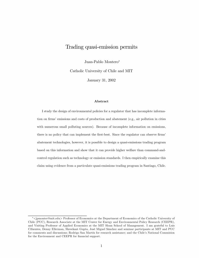
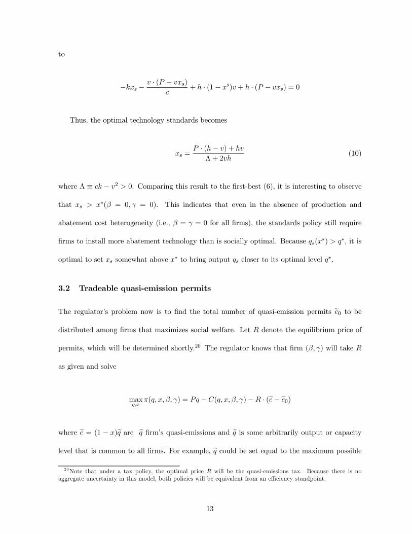
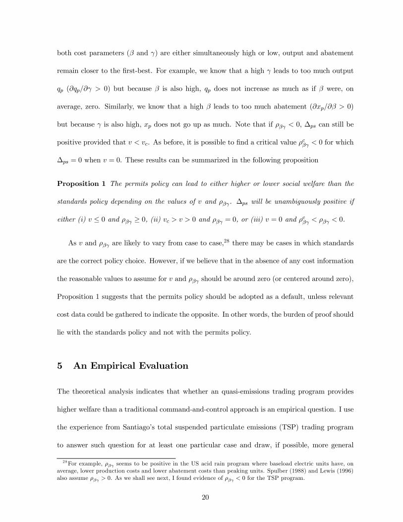
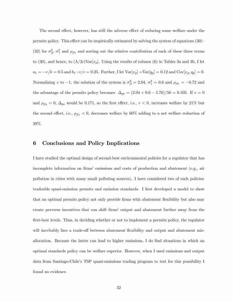
became e¤ective in 1994. Table 1 presents a summary of the data. The …rst two rows show that

the exit and entry of sources has been quite signi…cant. By 1999 36% of the a¤ected sources

were new sources despite the fact they did not receive any permits.

30For a full description of the program, see Montero et al. (2002).31PROCEFF is the government o¢ce responsible for enforcing the TSP program.32Since utilization has no e¤ect at all on the source’s compliance status, there is no reason to beleive that …rms

have incentives to misreport their true utilization. For the same reason, this information is available for mostbut not all sources.

22

In order to comply with the TSP trading program, a¤ected sources can hold permits, reduce

emissions or do both. They can reduce emissions by either decreasing their size (i.e., maximum

‡ow rate) or their emissions rates, through either fuel switching (for example, from wood,

coal, or heavy oil to light oil, liquid gas, or natural gas) or the installation of end-of-pipe

technology such as …lters, electrostatic precipitators, cyclones, and scrubbers. Sources do not

gain anything, in terms of emissions reduction, by changing their utilization level (i.e., days and

hrs of operation), because by de…nition it is assumed to be at 100%. Given that the authority

controls for the size of the source at the moment of permits allocation and emissions monitoring,

in terms of our theoretical model changes in emission rates would be captured by the variable

xp and utilization by the variable qp.

The next rows of Table 1 show data on ‡ow rates, emission rates and utilization. The

large standard deviations show that these three variables vary widely across sources in all

years.33 As the 1993 numbers indicate, sources’ utilization was quite heterogeneous before the

implementation of the program (a clear indication of a large ¾¯), indicating the potential for

higher emissions under a permits policy. Table 1 also indicates that the emissions rates of

a¤ected sources has remained quite di¤erent across sources after the program became e¤ective

(indication of a large ¾°). This compliance heterogeneity con…rms that, contrary to what occurs

under CAC regulation where all …rms must either install the same abatement technology or

comply with the same emissions rate xs, emissions-trading regulation provides enough ‡exibility

for sources to comply in very di¤erent ways.

The last two rows of Table 1 show data on total quasi-emissions and quasi-emissions per-

mits.34 Although 1994 was in principle the …rst year of compliance with the program, trading

33 It may seem strange to observe some ‡ow rates below the 1,000 (m3/hr) mark. In general, these areexisting sources for which their ‡ow rates were wrongly estimated above 1,000 (m3/h) at the time of registration.Nevertheless, these sources chose to remain in the program to keep the permits they had already received.34A few permits were retired from the market in 1997 as the authority revised the eligibility of some sources

to receiving permits (Montero et al., 2002).

23

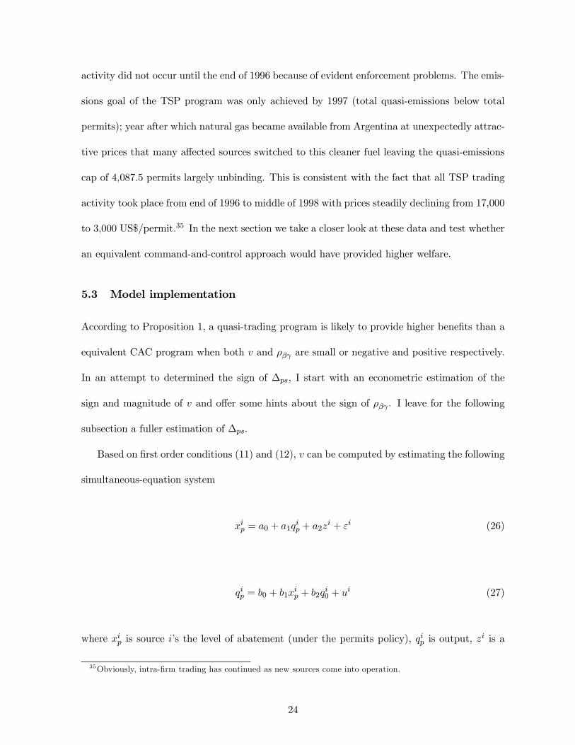
activity did not occur until the end of 1996 because of evident enforcement problems. The emis-

sions goal of the TSP program was only achieved by 1997 (total quasi-emissions below total

permits); year after which natural gas became available from Argentina at unexpectedly attrac-

tive prices that many a¤ected sources switched to this cleaner fuel leaving the quasi-emissions

cap of 4,087.5 permits largely unbinding. This is consistent with the fact that all TSP trading

activity took place from end of 1996 to middle of 1998 with prices steadily declining from 17,000

to 3,000 US$/permit.35 In the next section we take a closer look at these data and test whether

an equivalent command-and-control approach would have provided higher welfare.

5.3 Model implementation

According to Proposition 1, a quasi-trading program is likely to provide higher bene…ts than a

equivalent CAC program when both v and ½¯° are small or negative and positive respectively.

In an attempt to determined the sign of ¢ps, I start with an econometric estimation of the

sign and magnitude of v and o¤er some hints about the sign of ½¯° . I leave for the following

subsection a fuller estimation of ¢ps.

Based on …rst order conditions (11) and (12), v can be computed by estimating the following

simultaneous-equation system

xip = a0 + a1qip + a2z

i + "i (26)

qip = b0 + b1xip + b2q

i0 + u

i (27)

where xip is source i’s the level of abatement (under the permits policy), qip is output, z

i is a

35Obviously, intra-…rm trading has continued as new sources come into operation.

24

variable (or group of variables) that captures abatement costs so that a0+a2zi = Req=k¡°i=k,qi0 = (P ¡ ¯i)=c is output before the permits policy (i.e., TSP program) was implemented, and

"i and ui are error terms. Note that in the absence of other exogenous shocks to …rms’ behavior,

we should expect b0 = 0 and b2 = 1. The sign of v can be inferred from either a1 = ¡v=k or

b1 = ¡v=c. So, if a1, b1 ¸ 0 we will learn that v · 0 and that ¢ps is more likely to be positive

than otherwise.

Since I have information on xip and qip for a few years, I estimate the system (26)-(27) using

panel data regressions. I use 1995 as a reference year, that is a year before the TSP became

e¤ective. I use 1995 instead of 1993 because I have more complete information for 1995 and

because e¤ective enforcement with the TSP program did not begin until the end of 1996.36 The

basic speci…cation model is the following

REDUCit = a0 + a1UTILit + a2FLOWRTEit + a3EMRTE95i

+ a4ENDPIPEi + a5INDUSTi + a6STATEi + "it (28)

UTILit = b0 + b1REDUCit + b2UTIL95i + b3NATGASit + uit (29)

where i indexes sources; t indexes years; "it and uit are error terms whose characteristics will be

discussed shortly; and the chosen variables relate to those in (26)-(27) as follows. The variable

xp is captured by REDUC which is equal to the percentage reduction of a source’s emissions

rate, EMRTE, from its emissions rate in 1995, EMRTE95. Thus, source i’s reduction in

period t is given by REDUCit = (EMRTE95i ¡ EMRTEit)=EMRTE95i. Because I am

36See Montero et al. (2002). In any case, results do not qualitatively change when I use 1993 as the referenceyear.

25

taking EMRTE95 as a proxy for the rate that would have been observed in the absence of the

level TSP program (i.e., counterfactual rate), REDUC must be equal or greater than zero (by

construction cannot be greater than one as well) if input prices are assumed unchanged as in

our theoretical model. However, in a more general equilibrium setting where the relative price

of some dirtier inputs may go down after the introduction of the TSP program, it is possible

to observe a few sources for which REDUCit < 0.37

The variable qp is captured by UTIL which is a source’s utilization rate. As in the theoretical

model, TSP program’s authority does not observe UTIL, and therefore, she cannot use it for

monitoring and enforcement purposes. Put it di¤erently, because the regulator only observes

source’s ‡ow rate, FLOWRTE, and emissions rate, EMRTE, she has only control over changes

in emissions due to changes in source’s size (i.e., FLOWRTE) and emission rates but not over

changes in emissions due to changes in utilization.

FLOWRTE and the time-invariant variables EMRTE95, ENDPIPE, INDUST and

STATE and are intended to capture di¤erences in abatement costs across sources. If there

are any scale economies associated with pollution abatement we should expect more abate-

ment from bigger sources (i.e., larger FLOWRTE), other things equal.38 Similarly, I expect

that a source that starts from a high emission rate (i.e., high EMRTE95) should face more

abatement possibilities and hence lower costs. Conversely, I expect a source already equipped

with some end-of-pipe abatement technology required by previous regulation to be less likely

to reduce emissions. Hence, I introduce the dummy variable ENDPIPE that equals 1 if the

37 In cases of either lacking or obviously incorrect information on EMRTE95, I proceed as follows: I useEMRTE93 instead of EMRTE95 for 10 sources, EMRTE96 instead of EMRTE95 for 3 sources and eliminated7 sources for which their EMRTE have increased more than 50% relative to their counterfactual rate (i.e.,EMRTE95). Note that results do not change when I include 3 additional …rms for which EMRTE haveincrease between 50 and 100%. Results do substantially change when I include the 4 additional sources for whichtheir EMRTE’s have increased somewhere between 100 and 2500% times relative to their counterfactuals.38To address any endogeneity concerns about FLOWRTE, I run the same regressions with FLOWRTEit =

FLOWRTE95i for all t and obtain virtually identical results.

26

source has any type of end-of-pipe abatement technology by 1995. I also introduce the dummy

variables INDUST and STATE to see whether there is any di¤erence in abatement costs (or

abatement behavior) between industrial sources (INDUST = 1) and residential/commercial

sources, and between state or municipality owned sources (STATE = 1) and privately owned

sources.39 Since it is reasonable to think that privately owned and industrial sources should

be more responsive to changes in factor prices after the introduction of the TSP program than

other sources, I expect the coe¢cients of INDUST and STATE to be positive and negative,

respectively.

The variable UTIL95 in (29) is the source’s utilization in 1995 and serves as a proxy for

the level of utilization that would have been observed in the absence of the TSP program and

other exogenous factors. Although it does not follow directly from the theoretical formulation,

I also include UTIL95 in (28) for some regressions as a …rst attempt to explore the sign of ½¯° .

Because high levels of ex-ante output and ex-post abatement would tend to suggest a positive

correlation between production and abatement costs, the sign of the coe¢cient of UTIL95 in

(28) should serve as a …rst indication of the sign of ½¯°.40 Finally, NATGAS is a time-variant

dummy variable that equals 1 if the source is burning natural gas. Based on Montero et al.

(2002), who showed that the TSP program has had virtually no e¤ect on …rms’ decisions to

switch to natural gas, I include this variable to control for the lower production costs that

sources may enjoy after switching to this fuel. Since these lower costs should lead to higher

utilization, I expect the coe¢cient of NATGAS to be positive.

39For example, INDUST = 0 and STATE = 1 for the boiler of the central heating system of a public hospital.40Later I will determine the sign of ½¯° following an approach consistent with the theoretical formulation.

27

5.4 Econometric results

To estimate the coe¢cients in (28)-(29), I use a random-e¤ects model.41 Further, since UTIL

and REDUC enter as endogenous variables in (28) and (29), respectively, their correlations

with the error terms "it and uit would produce biased OLS estimators. Therefore, I employ

a generalized two stage least squares estimation procedure (G2SLS) to obtain unbiased esti-

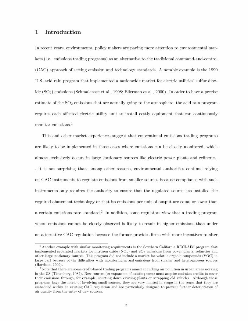
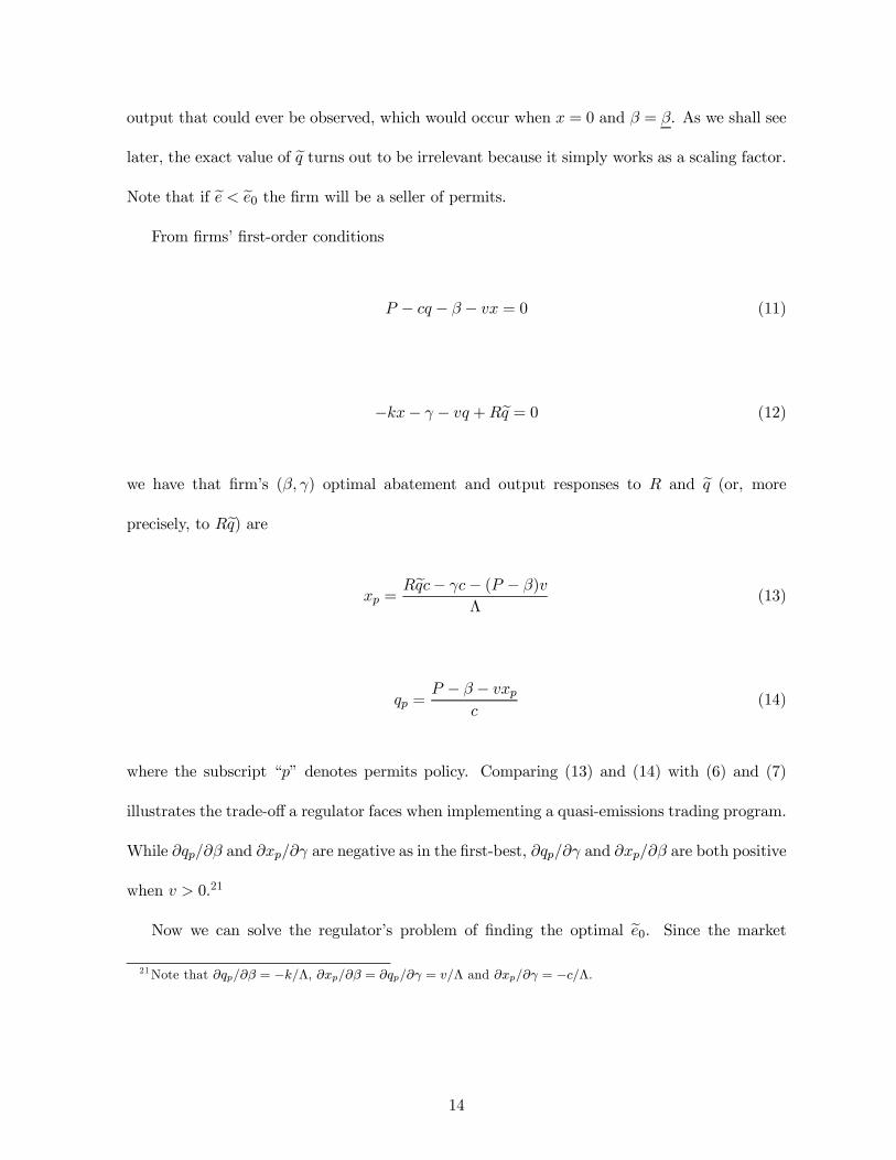
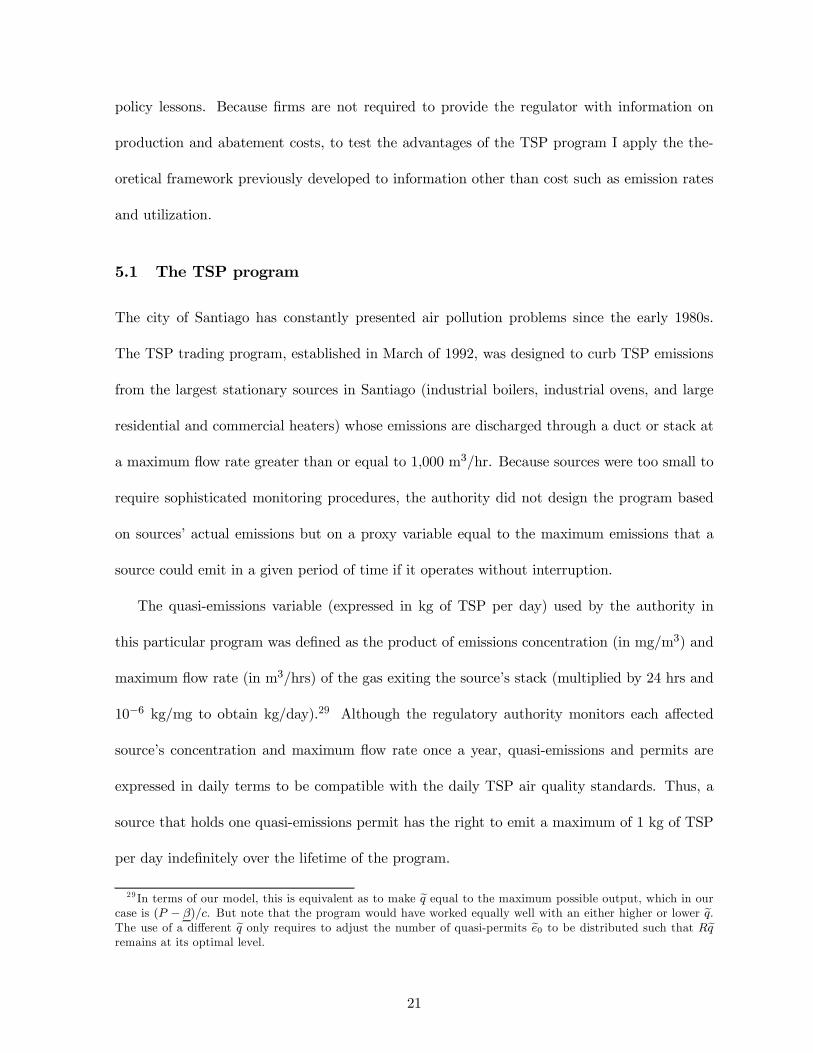
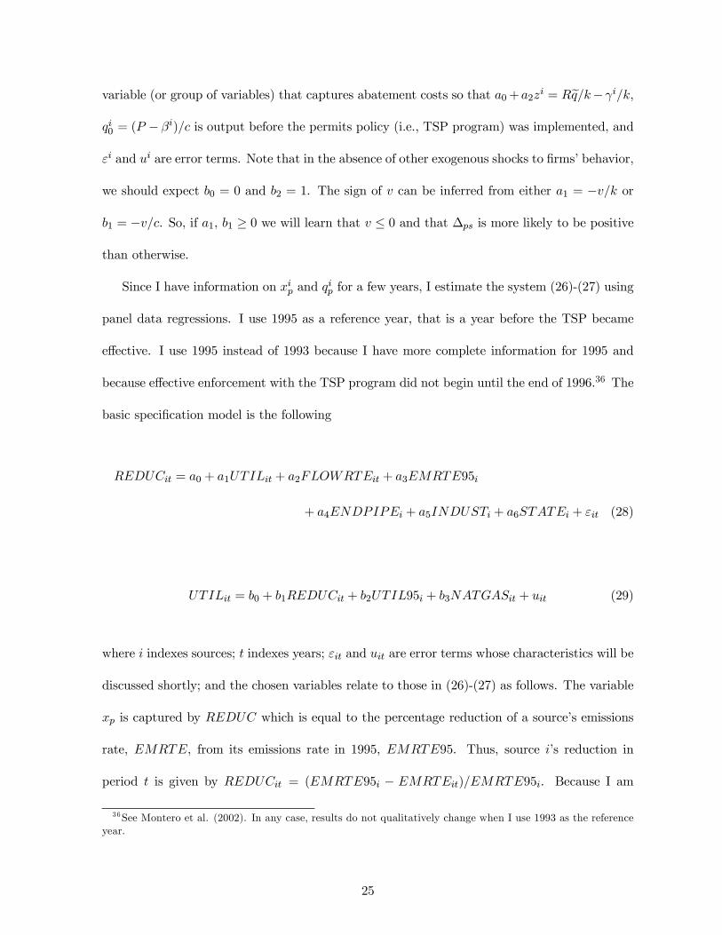
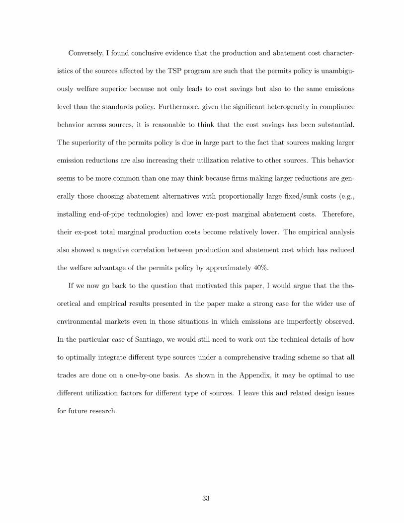
mates.42 Based on the data presented in Table 1, I construct a panel of 407 …rms for years 1996

through 1999.43 Since I do not have complete information for all …rms in all years the total

number of observations reduces to 1253. Summary statistics are reported in Table 2.

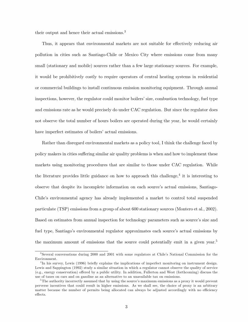
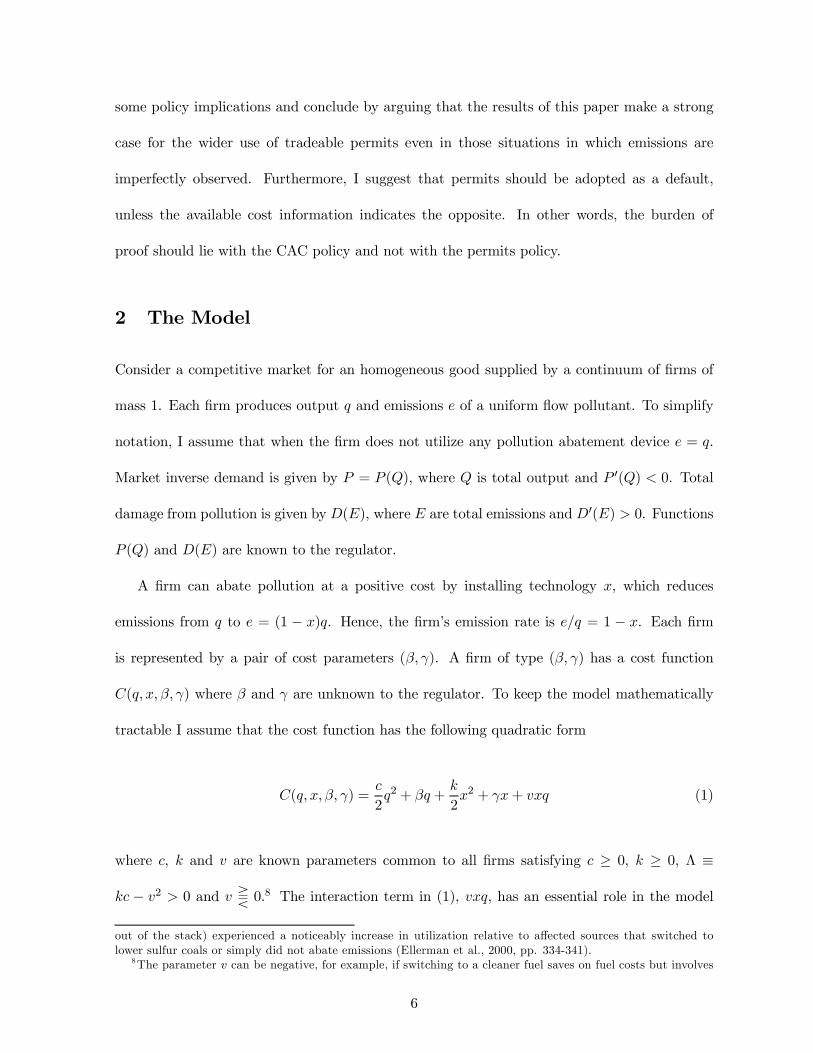
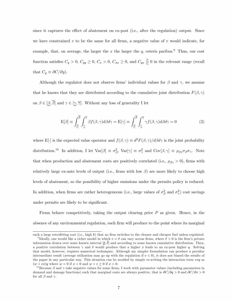
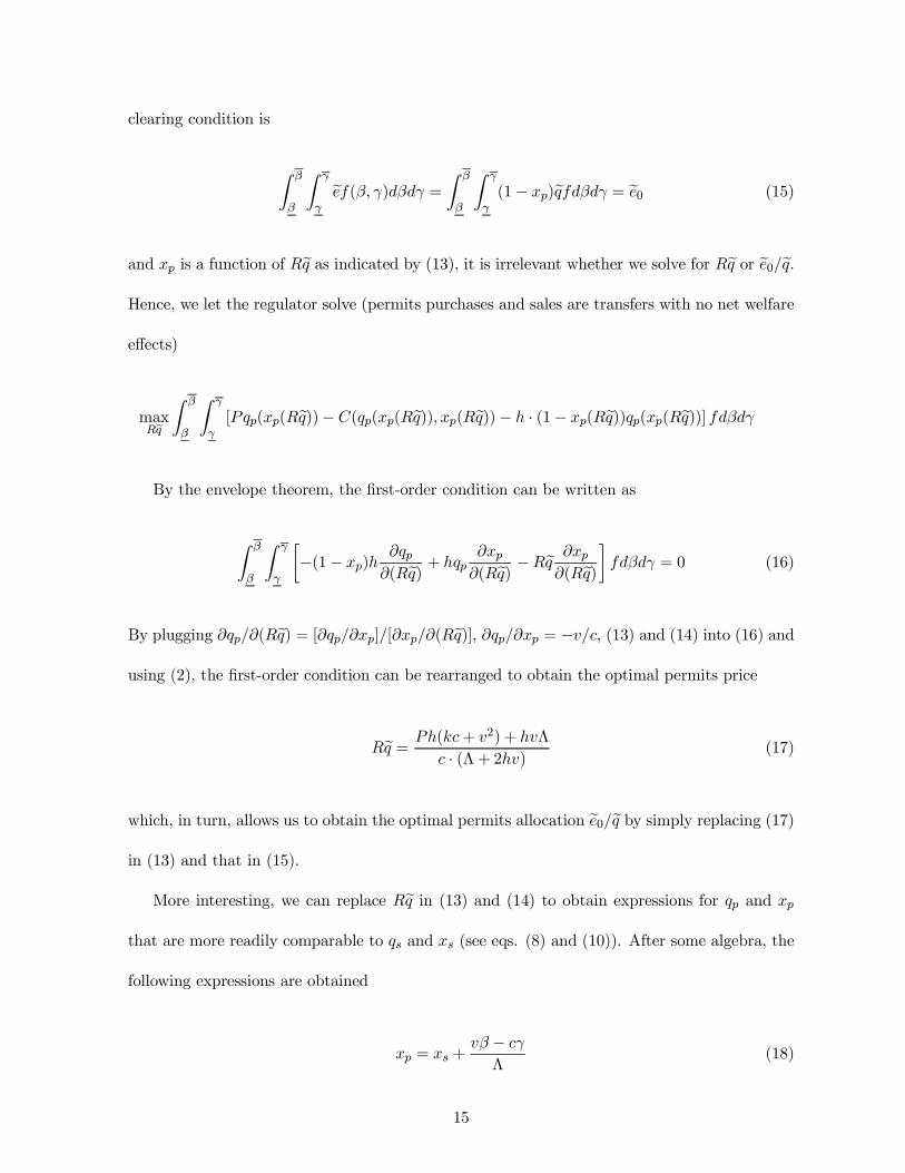
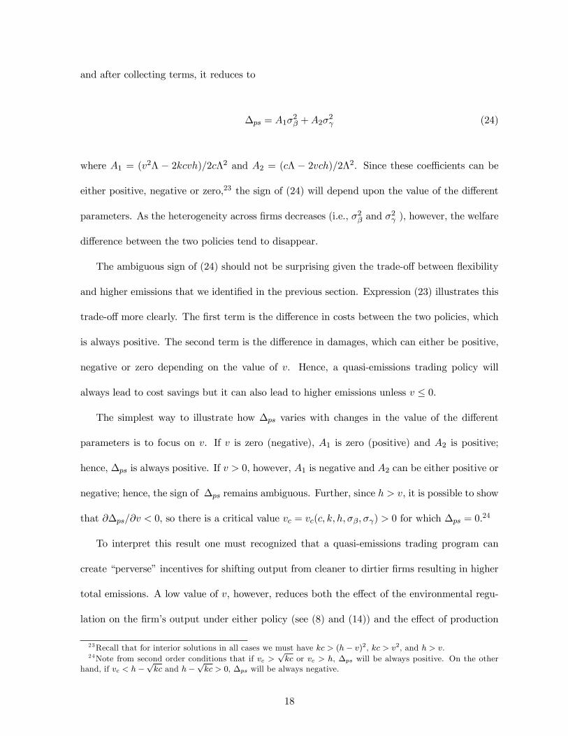
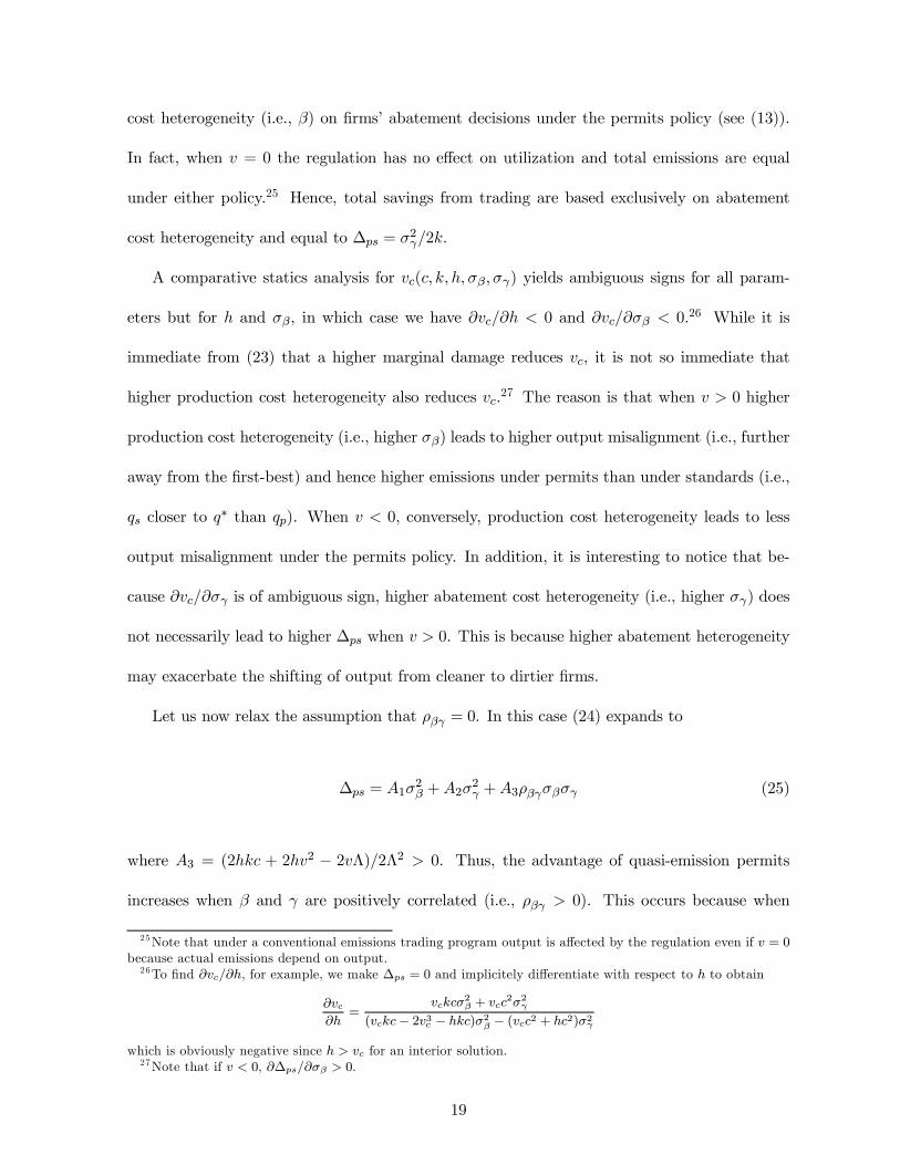
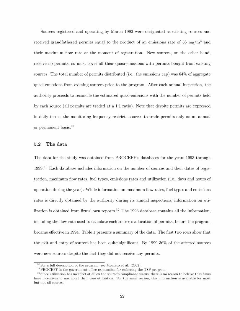
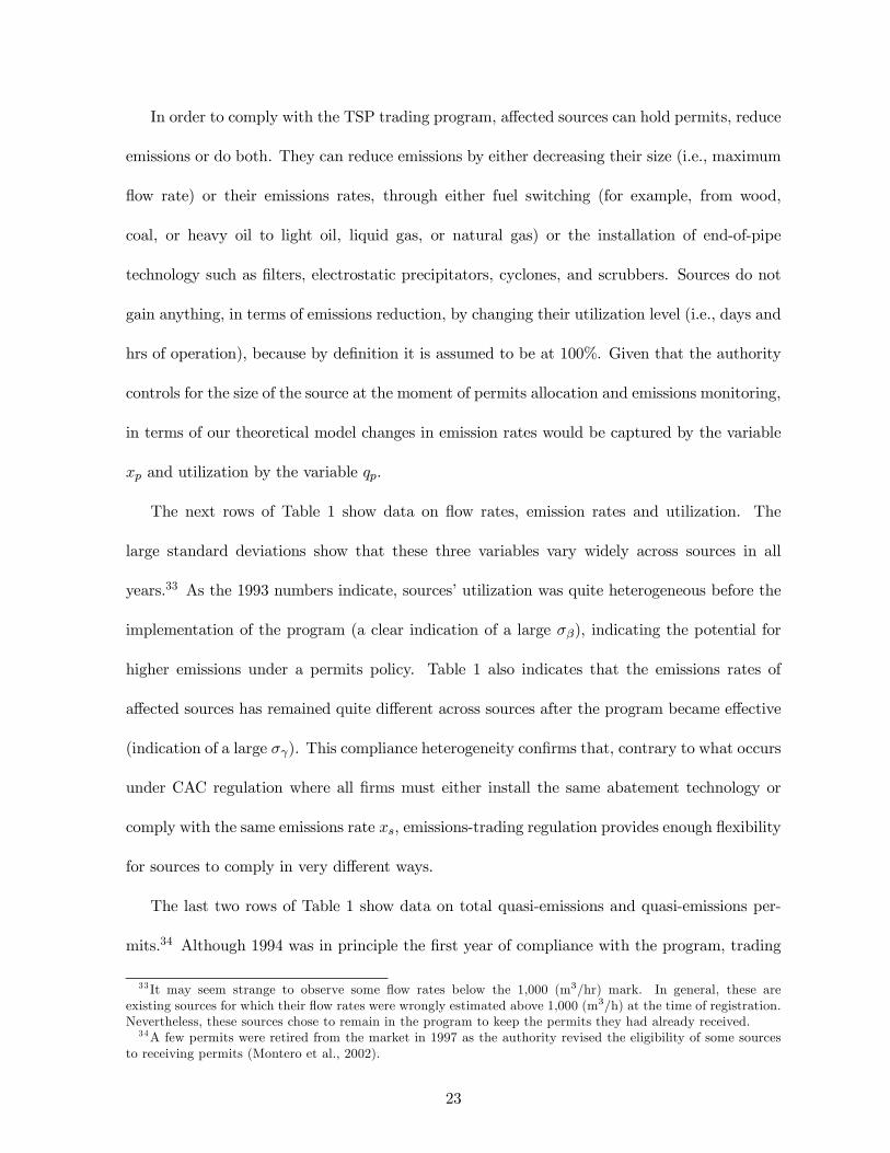
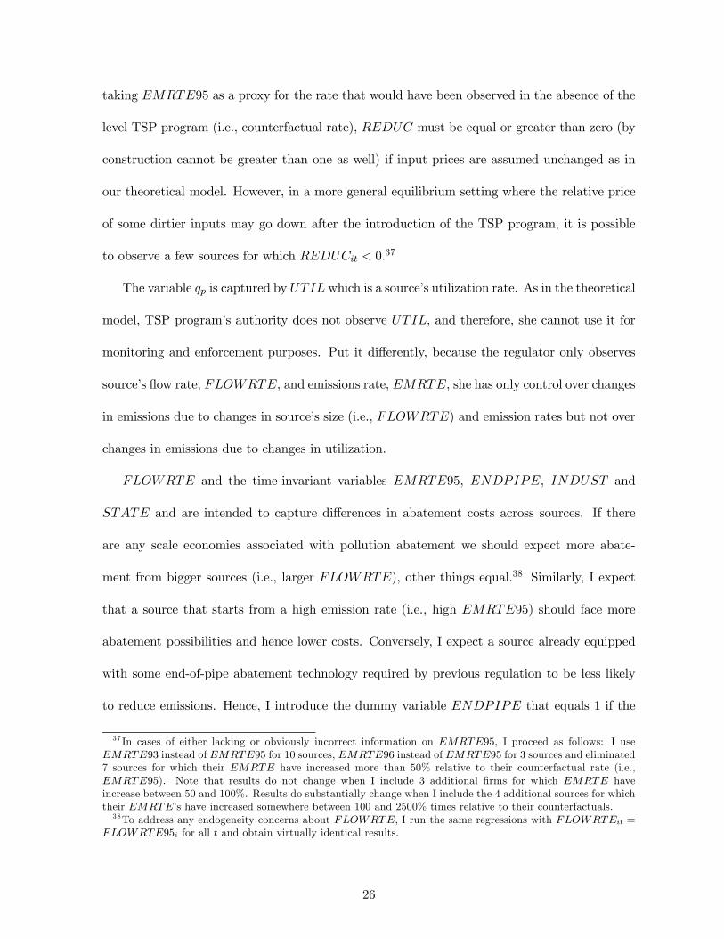
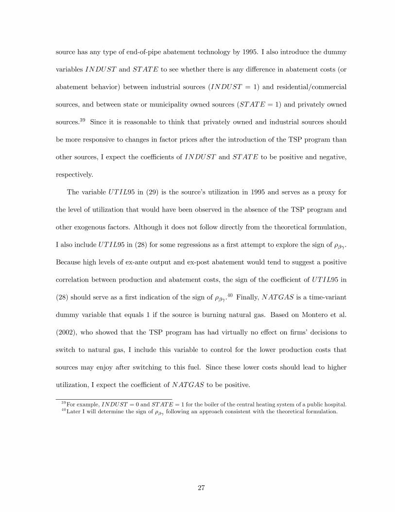
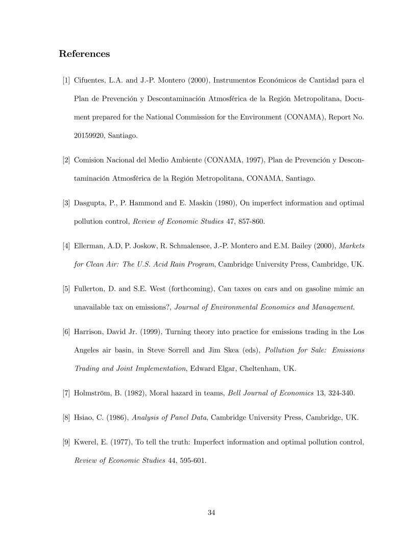
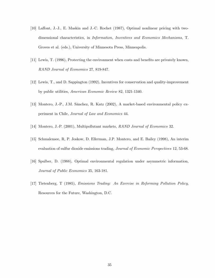
G2SLS results for both equations (28) and (29) are presented in Table 3a and 3b, re-

spectively (…rst-stage results are omitted). Results in column (1) show that the coe¢cients

of UTIL and REDUC (i.e., a1 and b1, respectively) are both positive and signi…cantly dif-

ferent from zero indicating not only that v < 0 but also that v is of important magnitude;

about 22% of k and 15% of c. Remaining coe¢cients in the utilization equation, UTIL95 and

NATGAS, have the expected sign but only UTIL95 is signi…cantly di¤erent from zero. In

addition, abatement cost coe¢cients in the reduction equation (i.e., FLOWRTE, EMRTE95,

ENDPIPE, INDUST , STATE) are signi…cantly di¤erent from zero and with the expected

signs except for FLOWRTE. Because there are a few sources with disproportionately large

values of FLOWRTE, in column (2) I replace FLOWRTE by its natural log, LOGFLOW ,

and in column (3) I include the dummy LARGEFLOW that equals one for 15 observations

in which FLOWRTEit > 50; 000 (bigger than more than three standard deviations from the

mean). Since results barely change, in what follows I use LOGFLOW .

41Note that using a …xed-e¤ects model it is not possible to estimate coe¢cients on time-invariant dummyvariables (e.g., STATE, INDUST ).42To obtain more e¢cient estimates I use Baltagi’s error-component two-stage least-squares (EC2SLS) method

(see Hsiao, 1986, pp. 97-127).43Note that I do not include new …rms that entered the market after 1995. Since I have 48 new …rms in the

sample, however, I was able to run regressions controlling for this characteristic and I found no e¤ects in theresults presented below.

28

In column (4), I include year dummies to control for exogenous factors that can a¤ect all

sources throughout the years (e.g., demand shocks, increase in enforcement capabilities, etc.).

While the coe¢cients of UTIL and REDUC remain positive and signi…cantly di¤erent from

zero, the coe¢cients of the year dummies in the reduction equation show a rather unilateral

reduction of emission rates overtime which can be attributed to a combination of more e¤ective

enforcement, availability of natural gas at low prices and the increase of emergency episodes

of bad air quality during which most polluting sources (i.e., those with higher emission rates)

must shut down operations momentarily.

In a further e¤ort to control for the evident increase in compliance after 1996, in column (5)

I present results for a panel of a subset of 360 …rms for years 1997 through 1999. Results are

similar to those in column (4) but for the size of coe¢cients of UTIL and REDUC that now

are much larger. Because trading activity did not take place until December of 1996 (Montero

et al., 2002), I think these latter numbers are better estimates of a1 and b1 in (28) and (29),

respectively.

Because our theoretical model assumes that all …rms are expected to produce, on average,

the same amount of output, E[qp] = (P ¡ vxs)=c, one can argue that our previous results

either underestimate or overestimate the true value of v by not taking into account the fact

that …rms are of di¤erent sizes (i.e., di¤erent FLOWRTE). One could further argue that the

true value of v is likely be smaller (in absolute terms) and perhaps positive because of the

negative sign of FLOWRTE (or LOGFLOW ). To explore this possibility, I treat each source

with FLOWRTE ¸ 1500 as a group of identical smaller sources of size FLOWRTE = 1000.

Accordingly, I replicate each observation in the 97-99 panel by the closest integer resulting from

the fraction FLOWRTEit=1000.44 The G2SLS results for this new panel of 4355 observations

44Each of the 12 observations for which FLOWRTE < 500 were retained as a single observation.

29

are in column (6).45

Finally, I provide a …rst approximation for the sign of ½¯° by including UTIL95 in (28).

Results are in column (7). The sign of UTIL95 shows that sources with large ex-ante utilization

are less likely to adopt high levels of abatement, suggesting a possible negative correlation

between production and abatement costs.

5.5 The value of ¢ps

The above results provide strong evidence that v < 0 and suggest that ½¯° may be negative.

Based on these results and Proposition 1 we cannot conclude whether ¢ps is positive or negative

yet. Nevertheless, I will use the econometric results below to estimate the magnitude of ¢ps.

From (18) and (19) it is immediate that

Var[xp] =1

¤2(v2¾2¯ + c

2¾2° ¡ 2vc½¯°¾¯¾°) (30)

Var[qp] =1

¤2(k2¾2¯ + v

2¾2° ¡ 2kv½¯°¾¯¾°) (31)

Cov[xp; qp] ´ E[xpqp]¡ E[xp]E[qp] = 1

¤2[(kc+ v2)½¯°¾¯¾° ¡ kv¾2¯ ¡ vc¾2° ] (32)

Note that (32) is the negative value of the di¤erence in total emissions, E, between the permits

and the standards policy, that is Ep ¡Es = ¡Cov[xp; qp]. In turn, eqs. (30) and (32) allow us

45 I also tried weighted 2SLS estimation methods (the weights are based on FLOWRTE’s) for di¤erent cross-sections with similar results.

30

to re-write ¢ps = A1¾2¯ +A2¾2° +A3½¯°¾¯¾° as

¢ps =¤

2cVar[xp] + hCov[xp; qp] (33)

As in (23), the …rst term in (33) is the di¤erence in costs savings between the permits

and the standards policies, which is always positive, while the second term, hCov[xp; qp], is the

di¤erence in environmental bene…ts.

The of sign of (33) the can be readily estimated by looking at the covariance matrix for

REDUC and UTIL. Using FLOWRTEit as a weight to control for size di¤erences across

sources, the weighted statistics for the 96-99 sample (1253 obs.) are Var[xp] = 0:115, Var[qp] =

0:110 and Cov[xp; qp] = 0:004, and the weighted statistics for the 97-99 sample (886 obs.) are

Var[xp] = 0:117, Var[qp] = 0:121 and Cov[xp; qp] = 0.46

Based on Cov[xp; qp] ¼ 0 and v < 0, we can immediately infer that ½¯° < 0 (see (32)).

More importantly, however, Cov[xp; qp] ¼ 0 allows us to conclude that Ep = Es and that

¢ps = (¤=2c)Var[xp] > 0. Thus, we can argue that the permits policy would unambiguously

provide higher welfare than the standards policy for any group of sources with a cost structure

similar to that of sources a¤ected by the TSP program. Furthermore, because Cov[xp; qp] = 0

the superiority of the permits policy would be independent of the aggregate emissions goal.

To understand why ¢ps > 0 requires to recognize the presence of two competing e¤ects.

While v < 0 increases the advantage of the permits policy by bringing output and abatement

closer to the …rst-best, ½¯° < 0 reduces such advantage by doing exactly the opposite. In the

case of the TSP program both e¤ects tend to cancel out so emissions would be similar under

either policy and ¢ps > 0.

46Unweighted statistics for the 96-99 sample are Var[xp] = 0:135, Var[qp] = 0:106 and Cov[xp; qp] = 0:021.While these …gures lead to a larger (and positive) ¢ps, they provide somehow baised estimates since bigger unitsare making relatively smaller reductions as indicated by the previous econometrics results.

31

The second e¤ect, however, has still the adverse e¤ect of reducing some welfare under the

permits policy. This e¤ect can be empirically estimated by solving the system of equations (30)–

(32) for ¾2¯, ¾2° and ½¯° and sorting out the relative contribution of each of these three terms

to (30), and hence, to (¤=2c)Var[xp]. Using the results of column (6) in Tables 3a and 3b, I let

a1 = ¡v=k = 0:5 and b1¡v=c = 0:25. Further, I let Var[xp] =Var[qp] = 0:12 and Cov[xp; qp] = 0.

Normalizing v to ¡1, the solution of the system is ¾2¯ = 2:04, ¾2° = 0:6 and ½¯° = ¡0:72 and

the advantage of the permits policy becomes ¢ps = (2:04 + 9:6 ¡ 5:76)=56 = 0:105. If v = 0

and ½¯° = 0, ¢ps would be 0:171, so the …rst e¤ect, i.e., v < 0, increases welfare by 21% but

the second e¤ect, i.e., ½¯° < 0, decreases welfare by 60% adding to a net welfare reduction of

39%.

6 Conclusions and Policy Implications

I have studied the optimal design of second-best environmental policies for a regulator that has

incomplete information on …rms’ emissions and costs of production and abatement (e.g., air

pollution in cities with many small polluting sources). I have considered two of such policies:

tradeable quasi-emission permits and emission standards. I …rst developed a model to show

that an optimal permits policy not only provide …rms with abatement ‡exibility but also may

create perverse incentives that can shift …rms’ output and abatement further away from the

…rst-best levels. Thus, in deciding whether or not to implement a permits policy, the regulator

will inevitably face a trade-o¤ between abatement ‡exibility and output and abatement mis-

allocation. Because the latter can lead to higher emissions, I do …nd situations in which an

optimal standards policy can be welfare superior. However, when I used emissions and output

data from Santiago-Chile’s TSP quasi-emissions trading program to test for this possibility I

found no evidence.

32

Conversely, I found conclusive evidence that the production and abatement cost character-

istics of the sources a¤ected by the TSP program are such that the permits policy is unambigu-

ously welfare superior because not only leads to cost savings but also to the same emissions

level than the standards policy. Furthermore, given the signi…cant heterogeneity in compliance

behavior across sources, it is reasonable to think that the cost savings has been substantial.

The superiority of the permits policy is due in large part to the fact that sources making larger

emission reductions are also increasing their utilization relative to other sources. This behavior

seems to be more common than one may think because …rms making larger reductions are gen-

erally those choosing abatement alternatives with proportionally large …xed/sunk costs (e.g.,

installing end-of-pipe technologies) and lower ex-post marginal abatement costs. Therefore,

their ex-post total marginal production costs become relatively lower. The empirical analysis

also showed a negative correlation between production and abatement cost which has reduced

the welfare advantage of the permits policy by approximately 40%.

If we now go back to the question that motivated this paper, I would argue that the the-

oretical and empirical results presented in the paper make a strong case for the wider use of

environmental markets even in those situations in which emissions are imperfectly observed.

In the particular case of Santiago, we would still need to work out the technical details of how

to optimally integrate di¤erent type sources under a comprehensive trading scheme so that all

trades are done on a one-by-one basis. As shown in the Appendix, it may be optimal to use

di¤erent utilization factors for di¤erent type of sources. I leave this and related design issues

for future research.

33

References

[1] Cifuentes, L.A. and J.-P. Montero (2000), Instrumentos Económicos de Cantidad para el

Plan de Prevención y Descontaminación Atmosférica de la Región Metropolitana, Docu-

ment prepared for the National Commission for the Environment (CONAMA), Report No.

20159920, Santiago.

[2] Comision Nacional del Medio Ambiente (CONAMA, 1997), Plan de Prevención y Descon-

taminación Atmosférica de la Región Metropolitana, CONAMA, Santiago.

[3] Dasgupta, P., P. Hammond and E. Maskin (1980), On imperfect information and optimal

pollution control, Review of Economic Studies 47, 857-860.

[4] Ellerman, A.D, P. Joskow, R. Schmalensee, J.-P. Montero and E.M. Bailey (2000), Markets

for Clean Air: The U.S. Acid Rain Program, Cambridge University Press, Cambridge, UK.

[5] Fullerton, D. and S.E. West (forthcoming), Can taxes on cars and on gasoline mimic an

unavailable tax on emissions?, Journal of Environmental Economics and Management.

[6] Harrison, David Jr. (1999), Turning theory into practice for emissions trading in the Los

Angeles air basin, in Steve Sorrell and Jim Skea (eds), Pollution for Sale: Emissions

Trading and Joint Implementation, Edward Elgar, Cheltenham, UK.

[7] Holmström, B. (1982), Moral hazard in teams, Bell Journal of Economics 13, 324-340.

[8] Hsiao, C. (1986), Analysis of Panel Data, Cambridge University Press, Cambridge, UK.

[9] Kwerel, E. (1977), To tell the truth: Imperfect information and optimal pollution control,

Review of Economic Studies 44, 595-601.

34

[10] La¤ont, J.-J., E. Maskin and J.-C. Rochet (1987), Optimal nonlinear pricing with two-

dimensional characteristics, in Information, Incentives and Economics Mechanisms, T.

Groves et al. (eds.), University of Minnesota Press, Minneapolis.

[11] Lewis, T. (1996), Protecting the environment when costs and bene…ts are privately known,

RAND Journal of Economics 27, 819-847.

[12] Lewis, T., and D. Sappington (1992), Incentives for conservation and quality-improvement

by public utilities, American Economic Review 82, 1321-1340.

[13] Montero, J.-P., J.M. Sánchez, R. Katz (2002), A market-based environmental policy ex-

periment in Chile, Journal of Law and Economics 44.

[14] Montero, J.-P. (2001), Multipollutant markets, RAND Journal of Economics 32.

[15] Schmalensee, R, P. Joskow, D. Ellerman, J.P. Montero, and E. Bailey (1998), An interim

evaluation of sulfur dioxide emissions trading, Journal of Economic Perspectives 12, 53-68.

[16] Spulber, D. (1988), Optimal environmental regulation under asymmetric information,

Journal of Public Economics 35, 163-181.

[17] Tietenberg, T (1985), Emissions Trading: An Exercise in Reforming Pollution Policy,

Resources for the Future, Washington, D.C.

35

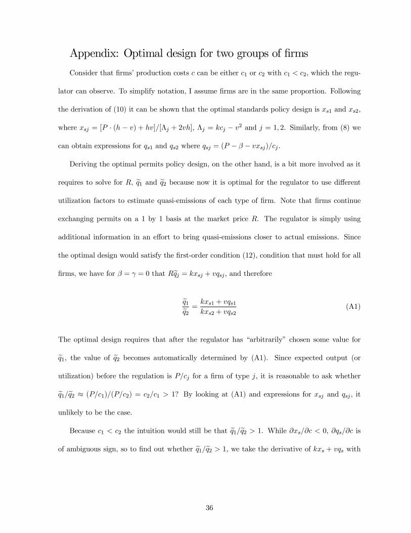
Appendix: Optimal design for two groups of …rms

Consider that …rms’ production costs c can be either c1 or c2 with c1 < c2, which the regu-

lator can observe. To simplify notation, I assume …rms are in the same proportion. Following

the derivation of (10) it can be shown that the optimal standards policy design is xs1 and xs2,

where xsj = [P ¢ (h ¡ v) + hv]=[¤j + 2vh], ¤j = kcj ¡ v2 and j = 1; 2. Similarly, from (8) we

can obtain expressions for qs1 and qs2 where qsj = (P ¡ ¯ ¡ vxsj)=cj .

Deriving the optimal permits policy design, on the other hand, is a bit more involved as it

requires to solve for R, eq1 and eq2 because now it is optimal for the regulator to use di¤erentutilization factors to estimate quasi-emissions of each type of …rm. Note that …rms continue

exchanging permits on a 1 by 1 basis at the market price R. The regulator is simply using

additional information in an e¤ort to bring quasi-emissions closer to actual emissions. Since

the optimal design would satisfy the …rst-order condition (12), condition that must hold for all

…rms, we have for ¯ = ° = 0 that Reqj = kxsj + vqsj , and thereforeeq1eq2 = kxs1 + vqs1

kxs2 + vqs2(A1)

The optimal design requires that after the regulator has “arbitrarily” chosen some value for

eq1, the value of eq2 becomes automatically determined by (A1). Since expected output (or

utilization) before the regulation is P=cj for a …rm of type j, it is reasonable to ask whether

eq1=eq2 ¼ (P=c1)=(P=c2) = c2=c1 > 1? By looking at (A1) and expressions for xsj and qsj , it

unlikely to be the case.

Because c1 < c2 the intuition would still be that eq1=eq2 > 1. While @xs=@c < 0, @qs=@c isof ambiguous sign, so to …nd out whether eq1=eq2 > 1, we take the derivative of kxs + vqs with

36

respect to c, which is given by

@(kxs + vqs)

@c= k

@xs@c

+ v@qs@xs

@xs@c

=¤

c

@xs@c

< 0 (A2)

which implies that eq1=eq2 > 1.

37

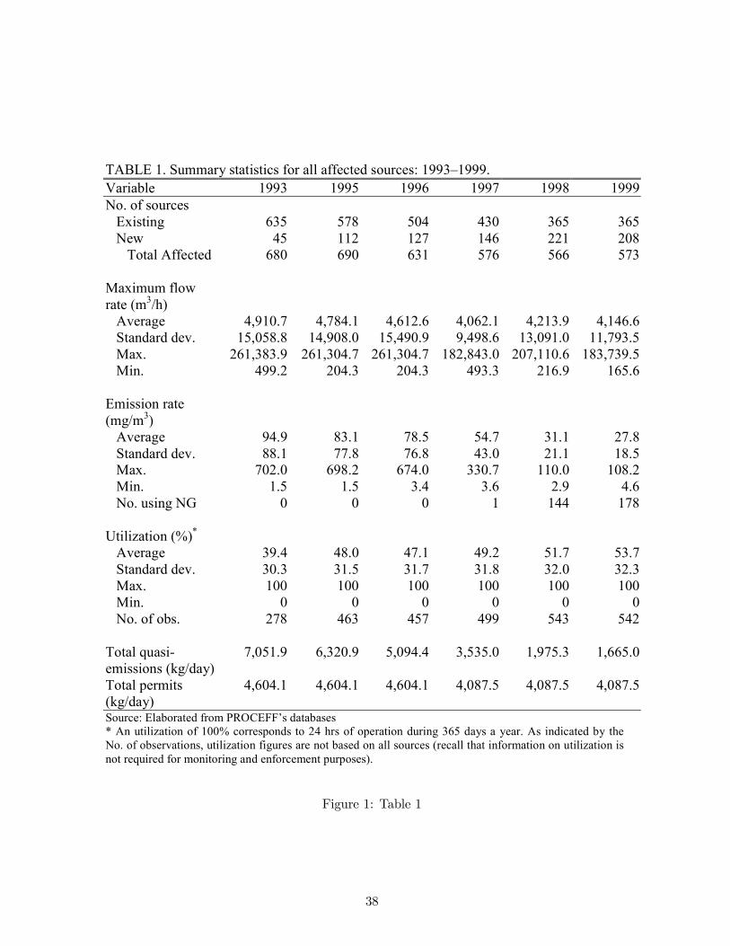
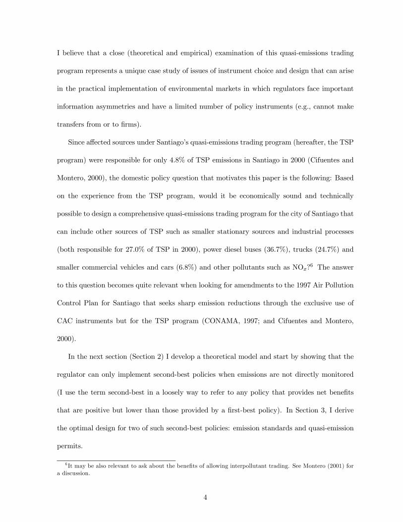
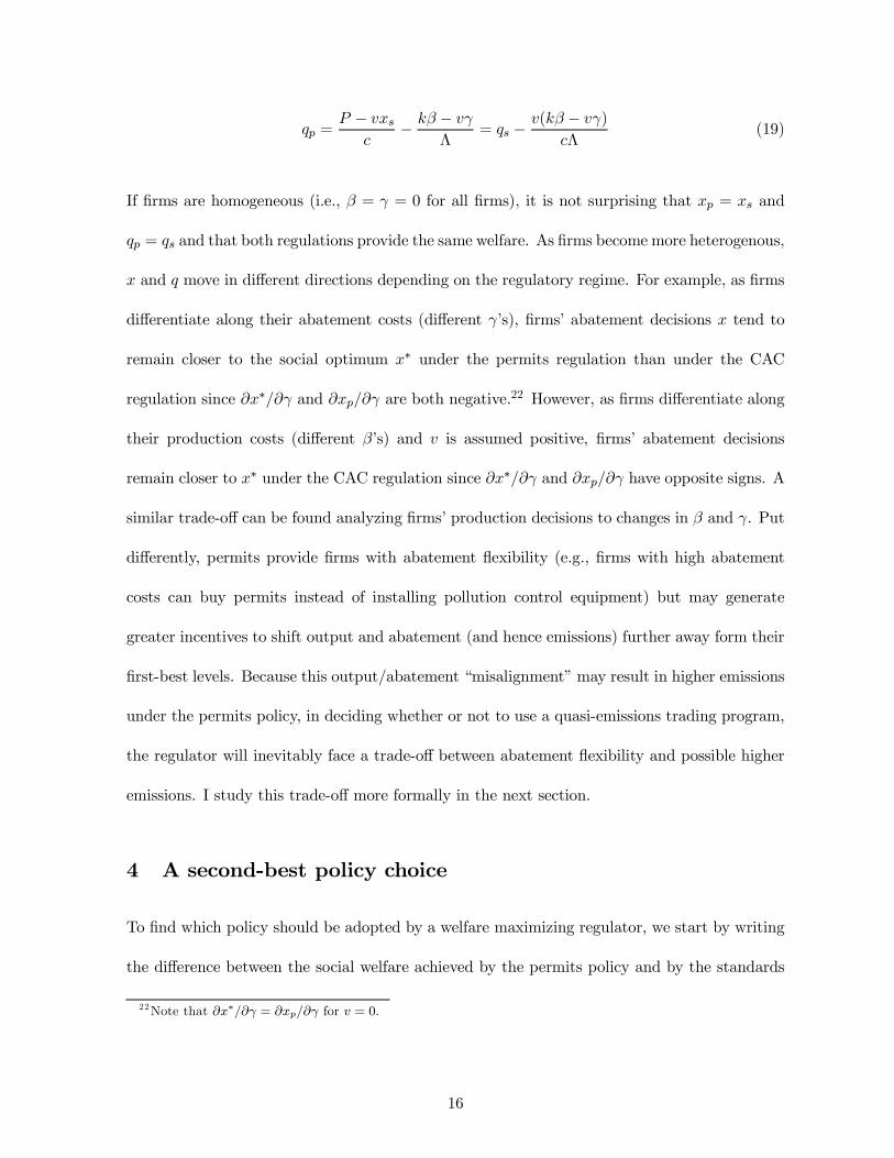
TABLE 1. Summary statistics for all affected sources: 1993–1999. Variable 1993 1995 1996 1997 1998 1999 No. of sources Existing 635 578 504 430 365 365 New 45 112 127 146 221 208 Total Affected 680 690 631 576 566 573

Maximum flow rate (m3/h)

Average 4,910.7 4,784.1 4,612.6 4,062.1 4,213.9 4,146.6 Standard dev. 15,058.8 14,908.0 15,490.9 9,498.6 13,091.0 11,793.5 Max. 261,383.9 261,304.7 261,304.7 182,843.0 207,110.6 183,739.5 Min. 499.2 204.3 204.3 493.3 216.9 165.6

Emission rate (mg/m3)

Average 94.9 83.1 78.5 54.7 31.1 27.8 Standard dev. 88.1 77.8 76.8 43.0 21.1 18.5 Max. 702.0 698.2 674.0 330.7 110.0 108.2 Min. 1.5 1.5 3.4 3.6 2.9 4.6 No. using NG 0 0 0 1 144 178 Utilization (%)* Average 39.4 48.0 47.1 49.2 51.7 53.7 Standard dev. 30.3 31.5 31.7 31.8 32.0 32.3 Max. 100 100 100 100 100 100 Min. 0 0 0 0 0 0 No. of obs. 278 463 457 499 543 542

Total quasi-emissions (kg/day)

7,051.9 6,320.9 5,094.4 3,535.0 1,975.3 1,665.0

Total permits (kg/day)

4,604.1 4,604.1 4,604.1 4,087.5 4,087.5 4,087.5

Source: Elaborated from PROCEFF’s databases * An utilization of 100% corresponds to 24 hrs of operation during 365 days a year. As indicated by the No. of observations, utilization figures are not based on all sources (recall that information on utilization is not required for monitoring and enforcement purposes).

Figure 1: Table 1

38

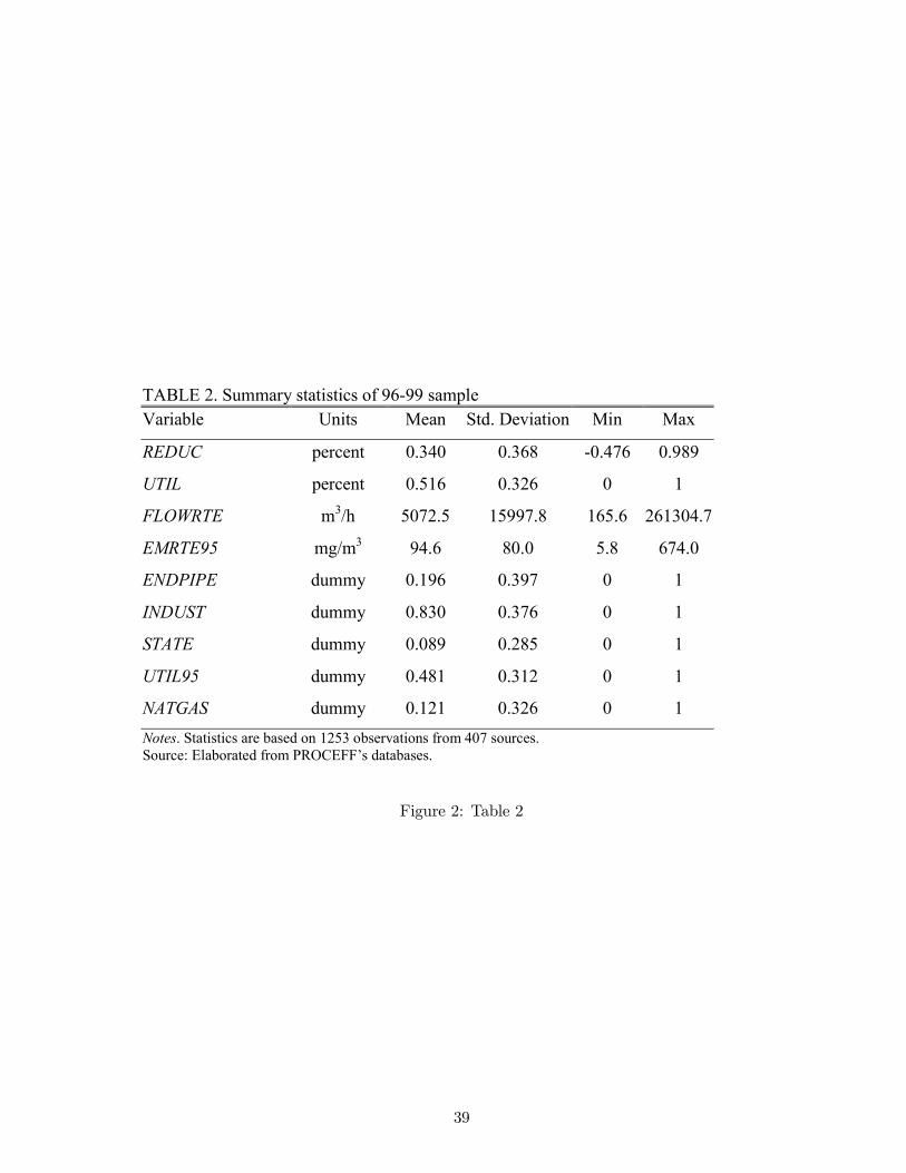
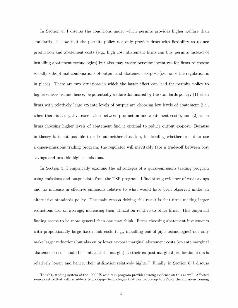
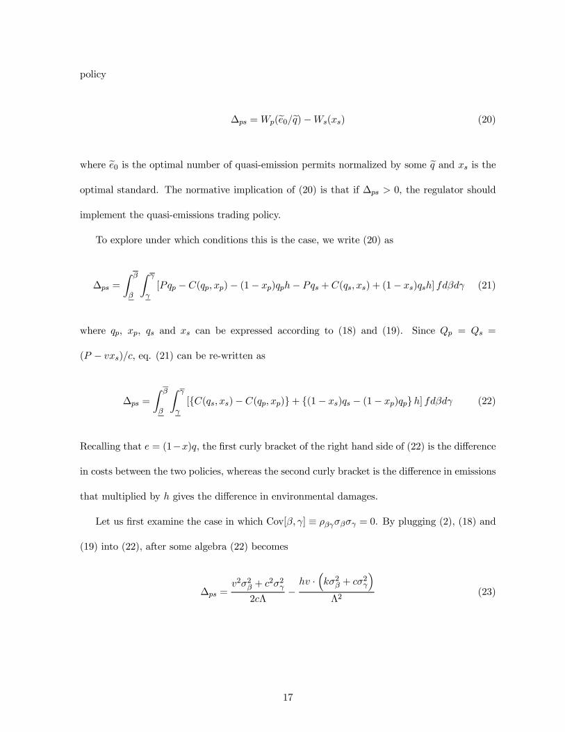
TABLE 2. Summary statistics of 96-99 sample Variable Units Mean Std. Deviation Min Max

REDUC percent 0.340 0.368 -0.476 0.989

UTIL percent 0.516 0.326 0 1

FLOWRTE m3/h 5072.5 15997.8 165.6 261304.7

EMRTE95 mg/m3 94.6 80.0 5.8 674.0

ENDPIPE dummy 0.196 0.397 0 1

INDUST dummy 0.830 0.376 0 1

STATE dummy 0.089 0.285 0 1

UTIL95 dummy 0.481 0.312 0 1

NATGAS dummy 0.121 0.326 0 1 Notes. Statistics are based on 1253 observations from 407 sources. Source: Elaborated from PROCEFF’s databases.

Figure 2: Table 2

39

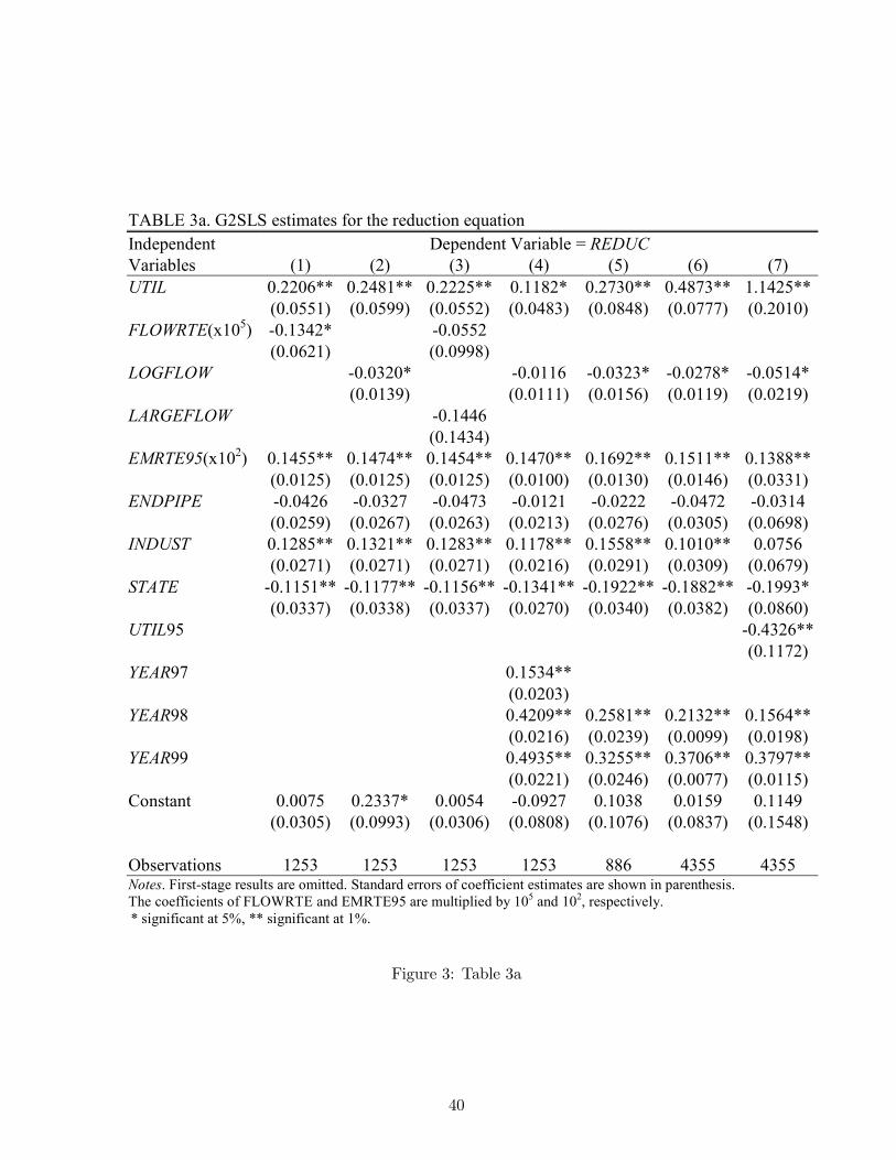
TABLE 3a. G2SLS estimates for the reduction equation Independent Dependent Variable = REDUC Variables (1) (2) (3) (4) (5) (6) (7) UTIL 0.2206** 0.2481** 0.2225** 0.1182* 0.2730** 0.4873** 1.1425** (0.0551) (0.0599) (0.0552) (0.0483) (0.0848) (0.0777) (0.2010) FLOWRTE(x105) -0.1342* -0.0552 (0.0621) (0.0998) LOGFLOW -0.0320* -0.0116 -0.0323* -0.0278* -0.0514* (0.0139) (0.0111) (0.0156) (0.0119) (0.0219) LARGEFLOW -0.1446 (0.1434) EMRTE95(x102) 0.1455** 0.1474** 0.1454** 0.1470** 0.1692** 0.1511** 0.1388** (0.0125) (0.0125) (0.0125) (0.0100) (0.0130) (0.0146) (0.0331) ENDPIPE -0.0426 -0.0327 -0.0473 -0.0121 -0.0222 -0.0472 -0.0314 (0.0259) (0.0267) (0.0263) (0.0213) (0.0276) (0.0305) (0.0698) INDUST 0.1285** 0.1321** 0.1283** 0.1178** 0.1558** 0.1010** 0.0756 (0.0271) (0.0271) (0.0271) (0.0216) (0.0291) (0.0309) (0.0679) STATE -0.1151** -0.1177** -0.1156** -0.1341** -0.1922** -0.1882** -0.1993* (0.0337) (0.0338) (0.0337) (0.0270) (0.0340) (0.0382) (0.0860) UTIL95 -0.4326** (0.1172) YEAR97 0.1534** (0.0203) YEAR98 0.4209** 0.2581** 0.2132** 0.1564** (0.0216) (0.0239) (0.0099) (0.0198) YEAR99 0.4935** 0.3255** 0.3706** 0.3797** (0.0221) (0.0246) (0.0077) (0.0115) Constant 0.0075 0.2337* 0.0054 -0.0927 0.1038 0.0159 0.1149 (0.0305) (0.0993) (0.0306) (0.0808) (0.1076) (0.0837) (0.1548) Observations 1253 1253 1253 1253 886 4355 4355 Notes. First-stage results are omitted. Standard errors of coefficient estimates are shown in parenthesis. The coefficients of FLOWRTE and EMRTE95 are multiplied by 105 and 102, respectively. * significant at 5%, ** significant at 1%.

Figure 3: Table 3a

40

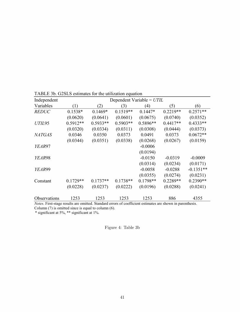
TABLE 3b. G2SLS estimates for the utilization equation Independent Dependent Variable = UTIL Variables (1) (2) (3) (4) (5) (6) REDUC 0.1538* 0.1469* 0.1519** 0.1447* 0.2219** 0.2571** (0.0620) (0.0641) (0.0601) (0.0675) (0.0740) (0.0352) UTIL95 0.5912** 0.5933** 0.5903** 0.5896** 0.4417** 0.4333** (0.0320) (0.0334) (0.0311) (0.0308) (0.0444) (0.0373) NATGAS 0.0346 0.0350 0.0373 0.0491 0.0373 0.0672** (0.0344) (0.0351) (0.0338) (0.0268) (0.0267) (0.0159) YEAR97 -0.0006 (0.0194) YEAR98 -0.0150 -0.0319 -0.0009 (0.0314) (0.0234) (0.0171) YEAR99 -0.0058 -0.0288 -0.1351** (0.0355) (0.0274) (0.0231) Constant 0.1729** 0.1737** 0.1738** 0.1798** 0.2289** 0.2390** (0.0228) (0.0237) (0.0222) (0.0196) (0.0288) (0.0241) Observations 1253 1253 1253 1253 886 4355 Notes. First-stage results are omitted. Standard errors of coefficient estimates are shown in parenthesis. Column (7) is omitted since is equal to column (6). * significant at 5%, ** significant at 1%.

Figure 4: Table 3b

41