Trading-off Volatility and Distortions?
49
Trading-off Volatility and Distortions? Economics and Politics of Food Policy During Price Spikes Hannah Pieters and Jo Swinnen LICOS – KU Leuven 2015 – FERDI Workshop 1 100 120 140 160 180 200 220 240 janv.-06 juil.-06 janv.-07 juil.-07 janv.-08 juil.-08 janv.-09 juil.-09 janv.-10 juil.-10 janv.-11 juil.-11 janv.-12 juil.-12 janv.-13 juil.-13 Food Price Index (2002-2004 =100)
Transcript of Trading-off Volatility and Distortions?

Trading-off Volatility and Distortions?
Economics and Politics of Food Policy During Price Spikes
Hannah Pieters and Jo Swinnen
LICOS – KU Leuven
2015 – FERDI Workshop 1
100
120
140
160
180
200
220
240
janv
.-06
juil.
-06
janv
.-07
juil.
-07
janv
.-08
juil.
-08
janv
.-09
juil.
-09
janv
.-10
juil.
-10
janv
.-11
juil.
-11
janv
.-12
juil.
-12
janv
.-13
juil.
-13
Food Price Index (2002-2004 =100)

Related literature includes e.g. …• Price Volatility and Stabilization
• Newberry and Stiglitz (1981)• Turnovsky et al (1980)• Gouel et al (2014, 2015)• Anderson, Ivanic and Martin (2013)• Barrett, Bellamare and Just (2013)• Minot (2014)
• Political Economy of Food Policy • Anderson (2009)• Anderson, Rausser and Swinnen (2013)• Rausser, Swinnen and Zusman (2011)
• Reactions to Price Spikes• Ivanic and Martin (2014)• Guariso, Squicciarini and Swinnen (2014)• Swinnen (1996, 2011)
• Politics and Economics of Instrument Choice• OECD (2011)• Swinnen (2009)• Swinnen, Olper and Vandemoortele (2011)

Everybody is Everybody is Everybody is Everybody is concerned about concerned about concerned about concerned about pricepricepriceprice volatilityvolatilityvolatilityvolatility (we thought …)
“The crux of the food price challenge is about price volatility, ratherthan high prices per se” (Kharas 2011)
“Food price levels are important, but so too is food price volatility. … it makes planning very difficult and … can lead to hunger and
malnutrition.”
Senior IFPRI researcher, Nov 2014 (Wall Street
“The EU’s Common Agricultural Policy [400 billion euro !] is a crucial instrument to provide a safety net for farmers in times of high price
volatility”
EU Commissioner for Agriculture, 2013

4
Rice markets and prices in China2006-2013

0
0,1
0,2
0,3
0,4
0,5
0,6ja
n/06
mar
/06
may
/06
jul/0
6se
p/06
nov/
06ja
n/07
mar
/07
may
/07
jul/0
7se
p/07
nov/
07ja
n/08
mar
/08
may
/08
jul/0
8se
p/08
nov/
08ja
n/09
mar
/09
may
/09
jul/0
9se
p/09
nov/
09ja
n/10
mar
/10
may
/10
jul/1
0se
p/10
nov/
10ja
n/11
mar
/11
may
/11
jul/1
1se
p/11
nov/
11ja
n/12
mar
/12
may
/12
jul/1
2se
p/12
nov/
12ja
n/13
mar
/13
may
/13
jul/1
3se
p/13
nov/
13
USD
/kg
INTERNATIONAL PRICES, USA: Gulf, Wheat (No. 2 Hard Red Winter), Export, (USD/Kg) Pakistan, Karachi, Wheat, Retail, (USD/Kg)5
Wheat markets and prices in Pakistan2006-2013
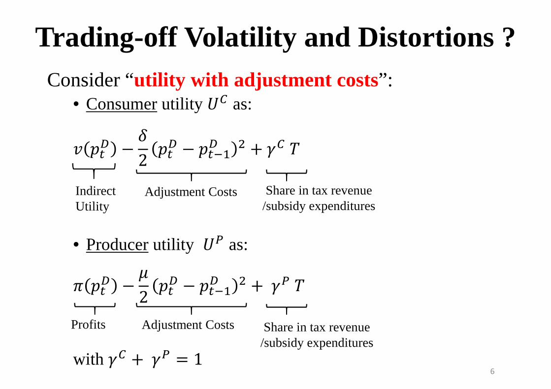
Trading-off Volatility and Distortions ? Consider “utility with adjustment costs”:
• Consumer utility �� as:
� ��� − �2 ��� − ���� � + �� �
• Producer utility �� as:
� ��� − �2 ��� − ���� � +���
with �� +�� = 1
Indirect Utility
Adjustment Costs Share in tax revenue /subsidy expenditures
Profits Adjustment Costs Share in tax revenue /subsidy expenditures
6

Socially optimal combination of volatility and distortions for a given price shock
7

But …. 1: Reviewer of the paper
•“ a long literature, notably Newbery and Stiglitz's 1981 book etc show that consumers may benefit from increased food price uncertainty ”

But … But … But … But … 2: Not everybody 2: Not everybody 2: Not everybody 2: Not everybody is is is is equally concerned equally concerned equally concerned equally concerned
about about about about pricepricepriceprice volatilityvolatilityvolatilityvolatility
• “Why food price volatility doesn’t matter”
(Barrett & Bellemare 2011)
• “Standard assessment of the welfare cost of food price volatility… suggest that … the cost to consumers is small if not negative. The only people who can expect significant gains from pricestabilization are the producers – and especially affluentproducers” (Christophe Goeul, 2013)
=> “Price stabilization is regressive” (i.e. benefits the rich)

Waugh (QJE 1944)

Waugh (QJE 1944)
Impact of price instability on consumer surplus
= G – L > 0

Oi (1961, Econometrica)

Samuelson (QJE 1972)

Samuelson (QJE 1972)

So: back to the drawing board …
• A new model based on Waugh, Oi, Newbery andStiglitz, Turnovsky et al, Barrett, Bellemare et al,Gouel et al, ….
• Following Barrett (1996):• a two-period model• product prices unknown when production decisions are
made• post-harvest prices announced before the consumer
makes its decision.

Consumer
����� � �(��, � • Maximization problem
• Benefit of price stabilization policy is analysed by looking at the Equivalent Variation
� �(�!, � + �") = � �(��, �)(Equivalent Variation measures consumer benefits of stabilization policy)
• Using Turnovsky et al. (1980) :
�" ≅ −� �%! ∙ �%� − �%! + ' ( − ) − * � �%! ∆,�-
-�%!
• ': budget share spend on food (. ≤ ' ≤ 0)• ): relative risk aversion of the consumer () ≥ .)• (: income elasticity of consumption (( ≥ .)
• * : price elasticity of consumption (* ≤ .)
Consumer
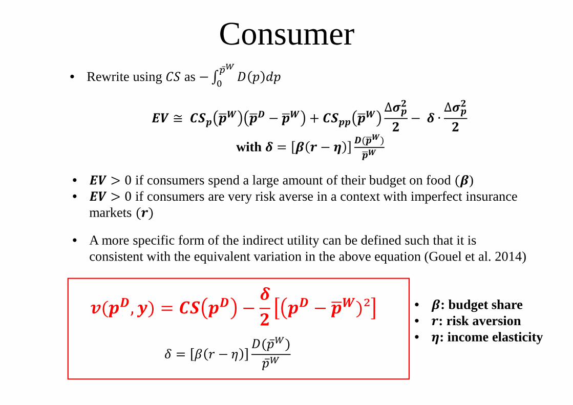
�" ≅ 23� �%! �%� − �%! + 23�� �%! ∆,�-
- − 4 ∙ ∆,�-
-with 4 = ' ) − ( �(�%!)
�%!
• �" > 0 if consumers spend a large amount of their budget on food (')• �" > 0 if consumers are very risk averse in a context with imperfect insurance
markets ())• A more specific form of the indirect utility can be defined such that it is
consistent with the equivalent variation in the above equation (Gouel et al. 2014)
�(��, �) = 23 �� − 4- 7�� − �%!)²
� = 9 : − ; <(�̅>)�̅>
• Rewrite using ?@ as −A < � B�C̅DE
• ': budget share • ): risk aversion • (: income elasticity

Producer
�" ≅ 3(�%) �%� − �%! − F G − ) + H ∙ ∆,�-
-�%!
• Equivalent Variation is approximated by:
�" ≅ �%� − �%! ����
− ���-��
∙ ∆,�-
• Using Barrett (1996); Bellemare et al (2013) :
• F: dominance of the food crop in the total production (. ≤ F ≤ 0)• ): relative risk aversion of the producer () ≥ .)• G: income elasticity of the marketable surplus (G ≤ .)
• H : price elasticity of the marketable surplus (H ≥ .)
• Rewrite:
�" ≅ I� �%! �%� − �%! + I�� �%! ∆,�-- − J ∙ ∆,�-
-
with K = F() − G) 3(�%!)�%!

Producer�" ≅ I� �%! �%� − �%! + I�� �%! ∆,�-
- − J ∙ ∆,�--
with J = F() − G) 3(�%!)�%!
• A more specific form of the indirect utility can be defined such that it is consistent with the equivalent variation in the above equation (Gouel et al. 2014):
�(��, �) = I �� − J- �� − �%! -
• �" > 0 when producers are highly dependent on the production of food for their incomeL
with μ = L(: − N) O(C̅D)C̅D
• F: dominance of the crop • ): relative risk aversion• G: income elasticity of the
marketable surplus (G ≤ .)

The government
• Policy intervention to stabilize prices (with budgetary implications T):
� = �� − �> (< �� − @ �� )
• Government maximizes social welfare
PQRCS?@ �� − �
2 �� − �̅> � + � �� − T2 �� − �̅> �
+ �� − �> (< �� − @ �� )

Social Optimum with Volatility and Adjustment Costs
• The social welfare maximizing domestic price ��∗ is determined by First order condition :
−< ��∗ − � ��∗ − �̅> + �� < ��∗ − @ ��∗
+�� ��∗ − �> <V ��∗ − @V ��∗ +
@ ��∗ − � ��∗ − �̅> +�� < ��∗ − @ ��∗
+�� ��∗ − �> (<V ��∗ − @V ��∗ )= 0
21
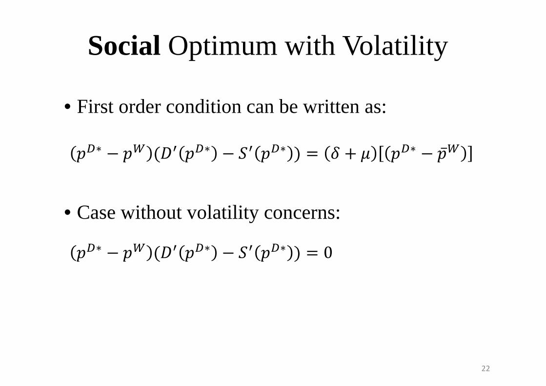
Social Optimum with Volatility
• First order condition can be written as:
• Case without volatility concerns:
��∗ − �> (<V ��∗ − @V ��∗ ) = � + � ��∗ − �̅>
��∗ − �> (<V ��∗ − @V ��∗ ) = 0
22

• First order condition can be written as:
or
Social Optimum with Volatility
��∗ = W�%! + 0 − W �!
withW = 4XJ4XJX3V�V ≥ . and . ≤ W ≤ 0
��∗ − �> = Y ��∗ − �̅>
with Y = ZX[�\OV = ]
]� ≤ 023

Social Optimum for different
24

• First order condition can be written as:
or
Social Optimum with Volatility
��∗ = ^�̅> + 1 − ^ �>
with^ = ZX[ZX[XOV�V ≥ 0 and 0 ≤ ^ ≤ 1
��∗ − �! = H ��∗ − �%!
with H = 4XJ�\3V = W
W0 ≤ .25

International price shocks and trade-off between distortions and volatility
26

Optimal combinations of observedvolatility and distortions for a givenprice shock
27

Empirical Evidence From developing countries
• Volatility (the coefficient of variation)
� = _�
• Distortions:
B = `1�
a
�bE��� − ��c
28

Distortions and volatility (2007-2013)
D (V=0): Minimum distortions at zero volatility V (D=0): Volatility at zero distortions (= world market price volatility)
29
Rice Wheat
Maize

Empirical Evidence Measuring the inefficiency of the actual
policy
Dis
tort
ion
Volatility
Vertical Distance
Horizontal Distance
Overall Distance
Country A
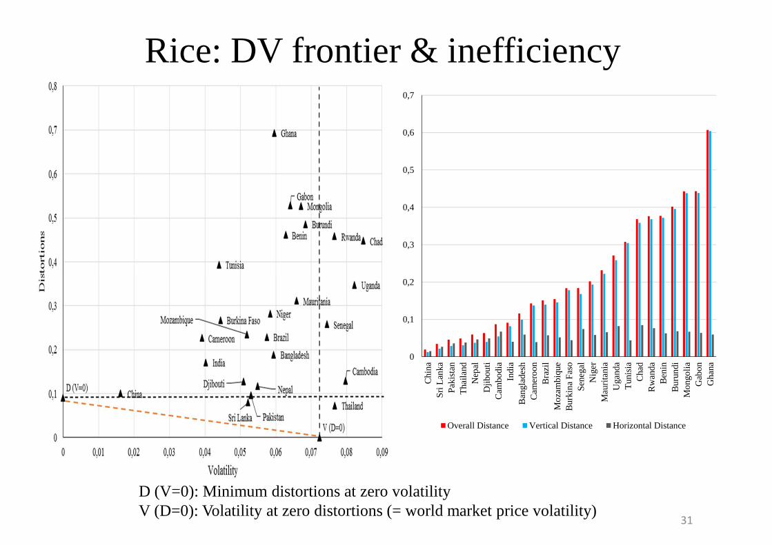
Rice: DV frontier & inefficiency
D (V=0): Minimum distortions at zero volatility V (D=0): Volatility at zero distortions (= world market price volatility)
31
0
0,1
0,2
0,3
0,4
0,5
0,6
0,7
Chi
na
Sri
Lan
kaP
akis
tan
Tha
iland
Nep
alD
jibou
tiC
ambo
dia
Indi
aB
angl
ades
hC
amer
oon
Bra
zil
Mo
zam
biq
ueB
urki
na
Fas
oS
eneg
alN
iger
Mau
rita
nia
Uga
nda
Tun
isia
Cha
dR
wan
daB
enin
Bur
undi
Mo
ngo
liaG
abon
Gha
na
Overall Distance Vertical Distance Horizontal Distance

WhyWhyWhyWhy sosososo muchmuchmuchmuch “policy “policy “policy “policy inefficiencyinefficiencyinefficiencyinefficiency” ? ” ? ” ? ” ? (even allowing for stability objectives)
Possible explanations:
1. Political determinants
2. Measurement problems
32

Political Optimum with Volatility and Adjustment costs
• Adjusted Grossman and Helpman (1994) model: the government maximizes:
PQRCS de?e(��) + dC?C(��) +f(��)
• de and dCare relative strength of the consumer and producer lobby
• ?e is the truthful contribution schedule of consumers• ?� is the truthful contribution schedule of producers• f(��) is social welfare
33

Political Optimum with Volatility
• First order condition :
34
��g − �! =hi ��g − �%!
− h ∙ 2i ∙ i + 2 ��g − �%!
+ �iX2 ��g − �%!
+� − 2 ∙ ji + 2
k = (� + �)
l = <V ��m − @V ��m
? = de�e + dC�C
< = d�� + d��
n = d�< ��m − d�@ ��m
o = < ��m − @ ��m
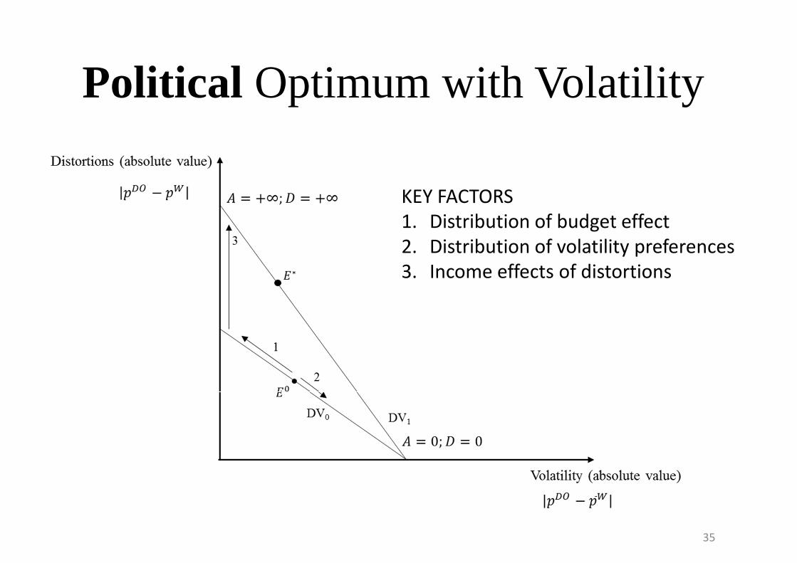
Political Optimum with Volatility
35
KEY FACTORS
1. Distribution of budget effect
2. Distribution of volatility preferences
3. Income effects of distortions

Let’s look at the correlation withsome empirical factors
Note:
• Almost all empirical indicators have a “politicaleconomy” aspect and a “measurement problem” aspect
• Observed distortions will reflect interaction of political influence and price moment
36

37
40.8
11.08
99.2
134.88
19.31
24.60
Distortions (2000-2005) Distortions (2007-2013)
MeasuredMeasuredMeasuredMeasured distortiondistortiondistortiondistortion, , , , politicalpoliticalpoliticalpolitical power, power, power, power, andandandand pricepricepriceprice movementmovementmovementmovement

DV Inefficiency & Absolute ea-NRA
38
Rice
Wheat
Maize

DV Inefficiency & Tax Revenues
39
Import/Export Subsidies
Import/ExportTariffs
Mean Overall Inefficiency 0.106 0.274Variance 0.014 0.024Observations 8 13Hypothesized Mean Difference 0df 18t Stat -2.795P(T<=t) one-tail 0.006t Critical one-tail 1.734P(T<=t) two-tail 0.012t Critical two-tail 2.101
Rice
Import/Export Subsidies
Import/ExportTariffs
Mean Overall Inefficiency 0.031 0.067Variance 0.000 0.003Observations 3 3Hypothesized Mean Difference 0df 2t Stat -1.161P(T<=t) one-tail 0.183t Critical one-tail 2.920P(T<=t) two-tail 0.365t Critical two-tail 4.303
Import/Export Subsidies
Import/ExportTariffs
Mean Overall Inefficiency 0.129 0.128Variance 0.008 0.004Observations 11 7Hypothesized Mean Difference 0df 16t Stat 0.030P(T<=t) one-tail 0.488t Critical one-tail 1.746P(T<=t) two-tail 0.976t Critical two-tail 2.120
MaizeWheat

Regression
40
Coefficients Standard Error P-valueAbsolute Ex-ante NRA 0.212 0.118 0.085Taxation indicator -0.062 0.051 0.234Intercept 0.113 0.033 0.002R-Square 0.120Observations 28
pqrsstutrqu�t = '0(r�_wxh)t+'-y���zt{qt +Ht
Taxation = 1 if the country has import or export tariffsAbsolute Ex-ante NRA is a measure for the power of lobby groups

DV Inefficiency & Import Share
41
Rice
Maize
Wheat

DV Inefficiency & Landlocked
42
Rice
Wheat Maize

Regression
43
Coefficients Standard Error P-valueAbsolute Ex-ante NRA 0.145 0.114 0.218Taxation indicator 0.001 0.056 0.989Net-Import share 0.032 0.031 0.310Landlocked 0.119 0.056 0.046Maize dummy -0.060 0.050 0.245Wheat dummy -0.095 0.061 0.132Intercept 0.101 0.044 0.033R-square 0.377Observations 28
|}~�����~}��� =9�(~Q_��k)�+9��QRQ���}� +9� |P��:��+ 9� �Q}B����~B�+9� f�~Q��+9��Q��~� + Y�
Taxation = 1 if the country has import or export tariffsAbsolute Ex-ante NRA is a measure for the power of lobby groupsLandlocked = 1 if country is landlockedNet-Import share = share of net imports in total trade

D (V=0): Minimum distortions at zero volatility V (D=0): Volatility at zero distortions (= world market price volatility)
44
0
0,1
0,2
0,3
0,4
0,5
0,6
Overall Distance Vertical Distance Horizontal Distance
Trading off distortions and
volatility in Chinese rice markets
Major inefficiencies in some countries

Concludingcomments
• Issues :
• How much “distortions” in the “distortion measures” ?
• Interaction of politics and price direction
• Policy instrument choice• Short run : “Fire Brigade Policy-Making” (Swinnen, 1996)
• Medium run : political economy / social optimum
• Long run: use different instruments (development-related)
• Overall implications ? • Ignoring externalities (Anderson et al argument) : how important ?
45

Concludingcomments
46

Derivation of utility function
47
����� � �(��, � • Maximization problem
• Benefit of price stabilization policy is analysed by looking at the equivalent variation
� �(�!, � + �") = � �(��, �)• Equivalent Variation is approximated by:
�" ≅ �%� − �%! ����
− ���-��
∙ ∆,�-
• Using Turnovsky et al. (1980) and Roy’s identity:
�" ≅ −� �%! ∙ �%� − �%! + ' ( − ) − * � �%! ∆,�-
-�%!
• Rewrite using ?@ as −A < � B�C̅DE with ?@C =�?@ ��⁄ = −<(�) and ?@CC =
−<C(�): �" ≅ 23� �%! �%� − �%! + 23�� �%! ∆,�-
- − 4 ∙ ∆,�-
-with 4 = ' ) − ( �(�%!)
�%!

Derivation of utility function
48
�" ≅ 23� �%! �%� − �%! + 23�� �%! ∆,�-
- − 4 ∙ ∆,�-
-with 4 = ' ) − ( �(�%!)
�%!
• �" > 0 if consumers spend a large amount of their budget on food• �" > 0 if consumers are very risk averse in a context with imperfect insurance
markets
• A more specific form of the indirect utility can be defined such that it is consistent with the equivalent variation in the above equation
�(��, �) = ?@ �� − �2 (�� − �̅>)²
� = 9 : − ; <(�̅>)�̅>

Political Optimum with Volatility
• First order condition can be written as:
49
��g − �! = hi + 2 ��g − �%! + �
i+ 2 ��g − �%! + � − 2 ∙ ji + 2
k = (� + �)
l = <V ��m − @V ��m
? = de�e + dC�C
< = d�� + d��
n = d�< ��m − d�@ ��m
o = < ��m − @ ��m