No. 8003

TRADE UNIONISM, IMPLICIT CONTRACTING,AND THE RESPONSE TO DEMAND VARIATION

IN U.S. MANUFACTURING*

by

James E. Pearce

April 1980

ResearchPaper

•~.~FEDERAL RESERVE BANK OF DALLAS

This publication was digitized and made available by the Federal Reserve Bank of Dallas' Historical Library (FedHistory@dal.frb.org)

No. 8003

TRADE UNIONISM, IMPLICIT CONTRACTING,AND THE RESPONSE TO DEMAND VARIATION

IN U.S. MANUFACTURING*

by

James E. Pearce

April 1980

ResearchPaper

•~.~FEDERAL RESERVE BANK OF DALLAS

No. 8003

TRADE UNIONISM, IMPLICIT CONTRACTING,AND THE RESPONSE TO DEMAND VARIATION

IN U.S. MANUFACTURING*

by

James E. Pearce

April 1980

This is a working paper and should not be quoted or re­produced in whole or in part without the written con­sent of the author. The views expressed are those ofthe author and should not be attributed to the FederalReserve Bank of Dallas or any other part of the FederalReserve System.

In the middle 1970's, economists studying the cyclical behavior

of labor markets began to focus more attention on temporary layoffs. One

factor stimulating interest in this topic was the recognition of the con­

tribution of variation in layoff unemployment to variation in the aggregate

unemployment rate. Between the second quarter of 1973 and the second quar­

ter of 1975, the fraction of the unemployed on layoff jumped from 10 per­

cent to 20 percent while the unemployment rate was rising from 4.9 to 8.7

percent. The apparent rigidity in wages and hours in the presence of large

variations in layoff unemployment also contributed to interest in a theo­

retical explanation for layoffs. The newer theories address the questions

raised by the prevalence of stable wage, variable employment practices by

distinguishing contract markets from spot, or auction, markets and explor­

ing the consequences of the durability of the typical employment relation­

ship. The most frequently cited studies have investigated these issues

from the perspective of risk shifting. The major alternative approach

looks to transactions costs. l

The emphasis on understanding the process that generates layoffs

has been well-placed. The contractin9 theories have provided some useful

perspectives from which to view the operation of a labor market subject to

frequent demand variation. There has been little new empirical evidence,

however, and further progress will require more detailed knowledge about

the manner in which these markets function. This paper presents an attempt

to expand this knowledge. It reports an analysis of the effects of the de­

cline in the demand for labor over the 1973-1975 recession on the wages,

hours, and layoff unemployment of production workers in manufacturing.

-2-

A study of these manufacturing workers is relevant to the con­

tract theories because they account for much of the average level of and

cyclical variation in layoff unemployment. In May of 1973, 40 percent of

those on layoff were manufacturing workers; two years later this figure had

risen to more than 60 percent. In addition, this market exhibits the key

attributes found throughout the contracting literature--low permanent sep­

aration rates, stable wages and hours, and frequent large shifts in de­

mand. Some of these Qualities can be found in the CPS. While layoff unem­

ployment among hourly production workers was rising from less than 1 per­

cent to more than 5.5 percent, their average workweek fell from 43.2 hours

to 41.2, and real wages declined 3.5 percent.2 Much of the fall in wages

was a consequence of a 4 percentage point rise in the rate of inflation in

the twelve months following May of 1973.

Concluding that the recession had no effect on nominal wage

growth would be premature, however, for the results reported below reveal a

surprisingly significant effect of industry demand shifts on hourly wages.

The analysis combines data from the May Current Population Surveys (CPS)

and the Bureau of Labor Statistics time series of employment by industry.

The CPS provides observations on the wages, hours, and employment status of

individuals in each year, and the latter source is used to construct mea­

sures of the shifts in each industry.

The CPS reveals that the experience of an individual worker de­

pended heavily on whether he was a member of a labor union. The 1975 lay­

off unemployment rate for union members was 6.5 percent, over 2 percentage

points higher than the rate for nonunion workers. The decline in union

real wages of 2.5 percent was only half as large as the decline in nonunion

-3-

wages. The paper investigates the possibility that this occurred because

union workers are concentrated in particular types of industries and finds

these differences too large to be accounted for by composition alone.3

Other conclusions reached include:

(1) Variation in the fraction of employees working overtime accounted

for the bulk of the vari ati on in hours worked;

(2) Variation in this fraction was larger among union members than

among nonunion workers; and

(3l A disproportionate number of the workers found on layoff had been

employed in large establishments, while the employees who expe­

rienced adjustments in their hours worked per week were more

likely to be working in small plants.

On the other hand, the analysis fails to uncover some relationships that

one might have expected to find--neither wages nor industry unionization

percentages display any association with the stochastic variability of in­

dustry employment.

Comparing the evidence with the details of competing theories of

labor market contracting suggests that risk shifting plays a minor role in

the response to cyclical demand shifts. The failure to establish a rela­

tionship between a stochastic variability in industry employment and any

measures of contracting influence casts serious doubt on the relevance of

risk shifting models. On the other hand, plant size does exhibit a signi­

ficant relationship with variables that can be construed as measures of

contracting strength, and this is interpreted as an indication that trans­

actions costs are a more important determinant of the behavior of this

labor market.

I. The Methods and Data

The introduction noted some differences in the experiences of

union and nonunion workers. A primary objective here is determining the

extent to which union-nonunion differences in the manifestations of cycli­

cal activity are attributable to factors other than composition. Do the

differences in the stability of wages and employment arise primarily from

the conditions and characteristics of the industries in which union members

are concentrated, or does the response to a given demand shock depend more

on whether the establishment is unionized? There are environmental factors

that predispose an establishment's employees to organize, and there is

variation in the size and timing of cyclical demand shocks across firms, so

answering this question requires one to have the abili~ to control for

differences in these factors. Although, for this purpose, it would be

desirable to use variables describing the environmental and demand condi­

tions in each individual's place of work, the CPS does not identify employ­

ers so precisely. Therefore, each employer is assumed to be adequately

described by average measures for the entire industry of which it is a

part.

The primary analytical tool used in this study is multiple re­

gression, in which the unit of observation is the individual worker. The

dependent variables reflect the individual's wage, hours worked, and em­

ployment status in the reference week for the May CPS. The right side of

the equation contains individual characteristics from the CPS record and

industry variables obtained from other sources and attached to the CPS re­

cord. The measure of demand conditions at the time the individual was ob­

served, one of the industry variables, is interacted with the union dummy

-5-

to allow estimation of separate effects of demand shifts on uni on and non­

uni on work ers.

There are several possible directions in which one could proceed

when devising a measure of cyclical demand shifts, and no one is clearly

superior to the others. The measure used here is based on industry emp10y­

ment. 4 This choice is essentially dictated by the properties of the micro­

data, which cover a short time interval and a broad cross section. The

industry variable in the CPS is sufficiently detailed to identify 73 sepa­

rate industries within manufacturing that can be matched with an industry

(or group of industries) for which an employment series can be obtained

from the BLS establishment data. From these series a measure of the state

of labor demand in May of each of the three years was constructed for each

of the industries.

A straightforward procedure was used to construct these mea­

sures. The log of employment was regressed on a set of seasonal dummy var­

iables, time, and time squared using monthly observations over a seven and

one-half year interval. The coefficients from that regression were then

used to predict the log of employment for the twelfth month following the

last observation in the interval. The difference between the actual and

predi cted val ues was used as the measure of the state of demand in that

industry at that time. Because the observations on the individual workers

were obtained in May, the regressions run to predict employment in May of

year t used a sample period that ran from December of year t-9 to May of

year t-l.

The principal variable used to capture differences in environ­

ments is an estimate of the number of production workers per establishment

-6-

in each industry. The estimate was computed from data in the 1972 Census

of Manufacturers. Industries with larger establishments are more heavily

unionized, and the bureaucracy characteristic of larger plants should have

some effect on the response to demand variation. Also, workers in large

plants may be more interdependent and may have skills that are more firm

specific.

The establishment size measure is the only environmental control

used in the analysis of adjustments in hours and employment. The wage

analysis contains two others. A measure of stochastic employment variabil­

ity is included to see if wages behave differently in industries with his­

torically unstable employment. Its value is the sum of squared residuals

from a quadratic trend regression (that included seasonal dummies) of the

log of industry employment over the period January 1958 to June 1975. The

other variable in the wage analysis, estimated from the May CPS, is the

percentage of male, full-time production workers in each industry who are

union members. It captures the effect of other factors correlated with

unionism that might affect the level or flexibility of wages.

Table 1 contains some statistics indicatin9 how the industry mea­

sures vary across CPS industry groups. The demand shift variables, labeled

prediction errors, show a very large decline in the demand for labor over

the period. Employment was above the level predicted from recent trends by

an average of 13.5 percent in May of 1973, but by 1975 it had fallen to 11

percent below trend. A comparison of the means of these shift and volati­

lity measures in the durable and nondurable sectors indicates that employ­

ment has been more stable in nondurables by a factor of about three. Es­

tablishments in nondurables are also slightly smaller and less heavily

unionized.

-7-

Table 2 shows the distributions of the industry variables after

their attachment to the records of the CPS. The unit of observation here

is the individual worker. The means of the shift measures for union and

nonunion workers are interesting, for they reveal that the concentrations

of workers in industries that experienced large reductions in employment

were about the same for both union members and nonunion employees. Thus,

the 1975 union-nonunion difference in layoff unemployment does not appear

to be a consequence of greater union penetration in the more volatile dura­

ble goods sector. The table does indicate a marked difference in the con­

centrations of the two types of workers in industries characterized by

large plants, however.

Section II discusses regression analysis of the behavior of real

wages. The May CPS reports the straight time hourly wage for workers who

were paid by the hour. The log of this value deflated by the consumer

price index is the dependent variable in the regression equations. Esti­

mates are reported based on a sample that pooled the data from all three

years and also from regressions run on data from each year separately.

Section III discusses two regressions, one for employment status

and the other for hours worked. Both use a Qualitative dependent variable

with values ranging from 1 to 3. The estimates reported are partial deri­

vatives obtained from maximum likelihood estimation of conditional logit

model s.

The employment status equation analyzes the determinants of the

probability that an individual will be disemployed. The dependent variable

distinguishes people on temporary layoff from those who have been dis­

charged permanently.5 Those unemployed or not working for other reasons,

-8-

such as illness or strikes, are not included in the sample. Table 3 shows

the percentages of workers in this sample unemployed due to job loss. As

one might expect, union members are less likely to be discharged, and this

raises the possibility that the larger rise in union layoff unemployment

over this period might have been caused by a larger proportion of disem­

ployed nonunion workers being discharged rather than laid off. The logit

model allows the investigation of this possiblity.

The dependent variable used in the analysis of variation in the

length of individuals' workweeks is somewhat unconventional. The May CPS

reports the number of hours each respondent works in a normal week as well

as the number of hou.rs he actually worked in the survey reference week.

Table 4 contains statistics on a variable designated "excess hours," which

is the difference between actual and normal weekly hours expressed as a

percentage of normal hours. The table reveals that the small and stable

mean for this variable conceals considerable hours variation for individual

workers. Over 30 percent of manufacturing employees did not work their

usual number of hours during the reference weeks of these surveys, and the

average deviation from the normal level was not trivial.

The stability across years of the means of the positive and nega-

tive values of this variable is quite remarkable. Presumably, it reflects

the presence of upper and lower bounds on hours worked. 6 When demand falls

temporarily, employers layoff workers and do not reduce hours further once

they have shortened the workweek to a certain point. When demand rises,

firms prefer to add to the number of workers rather than extend the work-

"week beyond some limit. This property of the variable complicates the

analysis; a regression directly employing excess hours as the dependent

-9-

variable yields estimates that are difficult to interpret, because they are

subject to truncation and selectivity biases. The variable does exhibit

some year-to-year variation, however, and the table indicates it is primar­

ily due to variation in the proportions of employees working more or fewer

hours than normal. Therefore, the hours equation reported in Section III

uses a qua 1itati ve dependent vari ab le whose val ue is determi ned by the si gn

of excess hours.

II. Analysis of Real Wage Rates

The wage equations discussed in this section contain a mixture of

standard and uncommon variables. In addition to the industry measures de­

scribed in Section I, the equations include age and its square, years of

schoo1i ng, and sets of dummi es capturi ng vari ance attri butab1e to differen­

ces in marital and union status, area population density, region, occupa­

tion, and state laws regarding the establishment of the union shop.? The

industry vari abl es and the ri ght-to-wOrK du111ll\Y are interacted wi th the

union membership dummy. Table A-I, appended, contains the coefficients of

the variables that are not of primary concern in this paper. Space does

not permit a thorough discussion of these estimates, but a few are suffici­

ently important to note briefly.

Some of the coefficients suggest the existence of union threat

effects of the type sought by Rosen (1969). The nonunion establishments

most susceptible to union organization are large, in heavily unionized in­

dustries, and in states that allow the union shop. To make the overtures

of union organizers less appealing, nonunion plants in these environments

appear to have an incentive to pay above-market wages. The estimates in

-10-

Table A-1 are consistent with this scenario. Nonunion wages are lower in

right-to-work states and positively related to establishment size and the

industry unionization rate, while the two former variables have no effect

on union wages. The coefficient of the latter interacted with the union

dummy indicates the union wage premium is a positive function of the extent

of union organization in the industry.

Table 5 displays the coefficients of primary interest estimated

using a sample that pooled the observations from all years. The figures in

the first column refer to an equation containing only a set of year dummies

to capture between-year wage variation. Their coefficients show an approx­

imately 5-percent decline in real nonunion wages. The interaction of the

year dummies with the union du~ shows an upward trend in the union wage

premium and, therefore, a smaller decline in real wages for union members.

The second column reports an equation containing both the set of

year dummies and the prediction error. The positive coefficient for the

prediction error indicates procyclic variation in nonunion wages, and the

negative coefficient of the interaction between the prediction error and

the union du~ indicates the response of union wages to be significantly

smaller than the response of nonunion wages. The sum of the two coeffi­

cients, labeled a1+a2 in the table, reveals procyclic variation in real

union wages. The year dummies in this specification show that nonunion

wages, after adjustment for year-to-year shifts in demand, did not decline

at all during 1973-74 and rose about 3 percent during 1974-75. The adjust­

ed union wage premium declined over the period, as adjusted union wages

fell in the first year and remained constant the second.

The figures in the third column refer to an equation containing

the prediction error without the year dummies. The coefficients indicate

-11-

significant procyclic wage variation for both groups. The estimates do

not, however, i ndi cate that wage sensiti vi ty to cycl i cal shifts was hi gh.

A shift in labor demand causing employment to drop from a level consistent

with a prediction error of 15 percent (the mean of the positive prediction

errors in 1973) to -15 percent (the mean of the negatives in 1975) would

cause nonunion real wages to fall 6 percent, or 0.15 1967 dollars. The

effect on union wages would be about one-fourth as large.

If short-run demand shifts and long run productivity trends were

the only influences on real wages, the duPllly variable coefficients in col­

umn 2 would show steaqy year-to-year growth. They do not, and the history

of the period contains at least part of the explanation. Consumer prices

rose 6 percent in the year preceeding May 1973. In the subsequent twelve

months the increase was 10 percent, and it fell slightly to 9 percent in

the year prior to May 1975. The jump in the rate of growth of prices prob­

ably accounts for much of the absence of growth during the first year in

adjusted nonunion wages and during both years for adjusted union wages.

Assume for the moment that the prediction errors fully capture

the effect of short-run shifts and that productivity growth and the change

in the path of prices were the only other factors influencing wages. The

effect of inflation on real union wages implied by these estimates is then

very large, and much higher and longer-lived than the effect on nonunion

real wages. For example, if trend growth is assumed to be 3 percent, then

the inflation change was responsible for 5.1 percentage points of the 5.4

percentage point reduction in real union wage growth during 1973-74 and

3.0 of the 3.7-percentage point drop the following year. Inflation's ef­

fect on nonuni on wage growth was 1imited to 3 percentage poi nts of the

5.5-percentage point reduction in 1973-74.

-12-

These are rough approximations, but the estimates of the effect

of the price level change on union wage growth are a little large for com­

fort. If nominal union wages are less sensitive to external shocks than

nonunion wages, then real union wages should show a relatively large re­

sponse to inflation and a relatively small response to short-run demand

shifts. ManY union contracts contain clauses providing automatic cost-of­

living adjustment, however, so one could expect to see a smaller impact far

from unanticipated price level movements than is suggested here.

Table 6 displays the results from estimating the coefficients

using data for each year separately, and it reveals one reason for the

small union wage response to demand shifts estimated with the pooled sam­

ple. The coefficients in Table 5 reflect both within-year and between-year

wage variation, and those in Table 6 indicate the prediction errors capture

much more within-year union wage variance in 1974 and 1975 than in 1973.

Thus, the estimates from the pooled sample may understate the actual union

wage response, so the effect of the inflation increase implied by the dummy

variable coefficients in column 2 may be too large.

The pattern of the response estimates found in Table 6 is inter­

esting for its causes as well as its effects. It may be at least partly a

consequence of the Nixon administration price control program. Comprehen­

sive government intervention into the wage determination process began with

the freeze on all wages and prices on August IS, 1971. In the following

November the freeze was replaced with a system of supervised wage and price

increases. During this "Phase II," which lasted through early 1973, the

wage increases of approximately 70 percent of the nation's workers were

subject to the approval of the Pay Board. Wage and price controls lasted

•

-13-

through April of 1974, but after Phase II the proportion of workers covered

declined steadily, and the supervision of wage setting grew less formal •

Thus, most of the wages observed in 1973 and some of those observed in 1974

were probably influenced by the price control program.

Traditional analyses of the effect of controls have focused on

the behavior of average wages. Most studies of the Nixon program using

this approach have found little effect.8 The dummy variable coefficients

in Table 5 support this conclusion. Controls could alter wage distribu­

tions without affecting economy-wide averages, however, by dampening the

response to short-run movements in demand. Workers in industries experi­

encing unusually high demand would be denied the larger raises market con­

ditions would otherwise bring about, and employers in low-demand industries

might feel that awarding an increase much below the maximum allowable would

cause morale problems. Such considerations would account for the relative­

ly small coefficients for the prediction errors computed using the 1973 and

1974 samples, when employment in most industries was above trend. Students

of the subject contend that wage controls have a larger impact on the union

sector, and that hypothesis is supported by the estimates in Table 6; the

1975 response is 2.6 times the 1973 response for union members and 1.4

times larger in the nonunion sector. But the period covered is short and

highly volatile, so any conclusions must be regarded as extremely tenta­

tive.

In any case, the cyclic response of union wages is considerably

smaller than the response of nonunion wages. These estimates do not iden­

tify the source of the response differential, however. Does the lower sen­

sitivity of union wages arise from unionism directly, or is it a conse­

quence of the environment in which union workers are most commonly found?

-14-

To answer this question, the prediction error variables were interacted

with the unionization rate, employment variability, and establishment size

variables in an equation similar to the one reported in column 3 of Table

5. The coefficients of interest are in Table 7. The estimates attribute

little of the response differential to the environment. The estimated re­

sponse of nonunion wages declines only 20 percent when the means of the in­

dustry variables for union members (from Table 2B) are substituted for the

means for nonunion workers (from Table 2A). A similiar exercise reduces

the union wage response by 10 percent. Establishment size is the most im­

portant variable.

A surprising result emerging from the wage analysis is the fail­

ure to find evidence that historic employment variability influences wage

levels. Theory predicts risk averse workers will demand a premium for ac­

cepting jobs in firms with histories of cyclically sensitive employment.

The coefficients of the measure of stochastic employment variability in

Table 5 do not show this to be the case, however. The elasticities are

small and positive for nonunion workers and small and negative for union

workers. In only one case is an estimated elasticity larger than its stan­

dard error.

III. Analysis of Adjustment in Employment and Hours

The logit models reported in this section contain fewer explana­

tory variables than the wage equations. These regressions contain only age

and its square, years of schooling, establishment size, the prediction er­

rors, and dummies for union membership and occupation. A lagged prediction

error measure is also included. This variable, which is the average of the

-15-

prediction errors for December through May of the previous year, is in­

cluded to investigate the possibilit¥ that an unusual level of employment

in one year might affect an individual's probability of being unemployed or

working more than usual when he is observed in the subsequent year. For

example, one would expect to find a smaller fraction of employees in an in­

dustry working overtime if their employers did an exceptionally large

amount of hiring in the previous year.

The tables in this section report derivatives of the probabili­

ties with respect to the independent variables. The tables show separate

estimates for union and nonunion workers. The calculation of these deriva­

tives is explained in the Appendix. The procedure requires the assignment

of values to each of the probabilities; the values used here were obtained

by evaluating the logit functions when the prediction errors are 0 and the

other independent variables are set equal to their means conditional on

union membership, and are included at the bottom of the tables containing

the derivatives. This provides estimates of the effect of the variables in

a steady state situation, i.e., a world that has experienced no recent

stochastic variation in employment. The logit coefficient estimates are in

the Appendix.

The employment status model indicates that cyclical variation in

union layoff unemployment exceeds variation in nonunion layoff unemployment

and that much of the difference cannot be attributed to either environment­

al differences or the more frequent use of discharges by nonunion employ­

ers. Table 8 contains the derivatives computed from the logit coefficients

in Table A-2. The contemporaneous prediction error derivatives imply that,

if union and nonunion workers were alike and equally numerous, changes in

-16-

the employment status of union members would account for about 60 percent

of the year-to-year variation in total job loss unemployment. Variation in

this unemployment among nonunion workers is almost equally divided between

layoffs and discharges, but 70 percent of the variation in union job loss

unemployment arises from layoffs. Variation in union layoff unemployment

alone is almost as great as variation in unemployment from both sources

combined for nonunion workers.

The other two industry variables also have a significant effect

on the employment status probabilities. The lagged prediction error deri­

vatives support the hypothesis that, within an industry, employment in one

year and unemployment in the subsequent year are positively correlated.

Firms that are well stocked with workers from the previous year's hiring

will have a larger fraction of employees on layoff and will be less reluc­

tant to discharge those who are redundant or poorly qualified. Establish­

ment size has little effect on an industry's job loss unemployment rate,

but it does influence the proportion of unemployed job losers who expect to

be recalled. Layoff unemployment is an increasing function of plant size,

but discharge unemployment declines as this variable rises. Establishment

size and the union membership dummy are responsible for most of the union­

nonunion differences in the steady-state probabilities shown at the bottom

of Table 8.

The remaining variables in the model performed much as one would

expect. Unemployment declines with age, and the magnitude of the effect of

this variable is smaller for older workers. Craftsmen, the most highly

skilled of the workers included in the analysis, experience slightly lower

-17-

unemployment rates. The schooling derivatives are somewhat more interest­

ing. They reveal that education has a stronger effect on discharge unem­

ployment than on unemployment from layoffs. If investment in firm specific

skills is an important determinant of an employer's choice to use layoffs

rather than discharges when reducing his workforce, then this finding sup­

ports the proposition, advanced by Oi (19621, that investment in general

skills is positively correlated with investment in specific skills.

In the hours regression, as in the employment status model, the

industry variables provide the most interesting information. Table 9 re­

ports the derivatives computed from the coefficients listed in Table A-3.

The estimates reveal that cyclical variation in the fraction of employees

working overtime is large relative to variation is in the fraction working

short weeks. The lagged and contemporaneous prediction errors have a much

greater effect on overtime than on short time for both union and nonunion

workers. Another striking feature is the importance of the lagged predic­

tion error. The derivatives indicate that the influence of the previous

year's hiring on the probability of working the usual number of hours is

about as great as that of current demand conditions. The sign of the rela­

tionship corresponds with what one would expect: high employment in one

year reduces the following year's percentage of employees working overtime

and raises the percentage that will be working less than usual.

The hours model also indicates that employees in industries char­

acterized by large plants are less likely to experience hours variation

in a steady state situation. Both derivatives with respect to establish­

ment size in Table 9 are negative and statistically significant, so season­

al and other very short-lived shifts affect the hours of fewer workers in

-18-

larger establishments. A comparison of Tables 8 and 9 suggests that this

variable has more influence on the adjustment of hours than employment.

When stochastic shifts occur, union members are more likely to

experience hours adjustment than nonunion workers. The contemporaneous

prediction error derivatives are more than twice as large for union mem­

bers, and the difference is particularly large for the probability of work­

ing overtime. The remaining derivatives in this model reveal nothing ex­

ceptional. Older workers, those with more schooling, and craftsmen are

more likely to be observed working overtime and/or less likely to report a

short workweek. Thus, these variables indicate a positive relationship be­

tween skill and excess hours.

IV. Interpreting the Results

Other studies of the effect of unionism on the response to demand

variation have reported findings similar to those discussed above. Several

studies, beginning with Lewis (1963), analyzed aggregate time series data

and found that union wages respond less to cyclical shifts than nonunion

wages. Medoff (1979) found a positive relationship between the unioniza­

tion and layoff rates in state-industry cells. Raisian analyzed data from

the Michigan Panel Study of Income Dynamics using a technique similar to

the one here. The only major discrepancy between his results and those

discussed above is his finding of countercyclical movement in union wages.

Raisian's sample included workers from all industry groups, however.

The major advantage of this study is that the evidence presents a

stronger argument for the case that unionism itself affects the firm's re­

sponse to demand variation. The previous studies are unlikely to convince

-19-

the skeptical that the effects attributed to unionism are not a consequence

of a correlation between union or9anization and demand variability. Of

course, the possibility exists that such a correlation produced the results

obtained in this study also, but it is smaller.

If one accepts the conclusion that the union-nonunion differences

are due to unionism rather than the environment in which union members are

concentrated, then the explanation for this becomes an interesting ques­

tion. Medoff calls attention to the political aspects of union decision

making and to Freeman's (1978) application to the labor market of Hirsh­

man's exit-voice approach. The key point in this view is that the prefer­

ences of senior workers have more weight, relative to those of junior work­

ers, in the determination of conditions of employment under collective bar­

gaining than when the workforce is not organized. Because senior workers

are the last laid off and the first rehired, they will be affected less by

demand variation if the firm relies heavily on employment adjustment when

demand shifts. One of the consequences of unionization is, therefore, that

the employer will perceive greater desire among workers for layoffs and

rehires and less desire for flexible wages.

Raisian attempts to interpret his results within the context of

the recent literature on implicit contracting, which examines the circum­

stances surrounding the durable associations between many employers and

their employees. The labor market is dichotomized into auction and con­

tracting segments, and the behavior of the two is compared. Contract mar­

ket employers must be conscious of their reputations, for their treatment

of current employees affects their ability to recruit workers in the fu­

ture. This concern shapes the contract employer's response to demand

-20-

variation. Raisian contends that his evidence suggests that unionized em­

ployers behave as if they were in the contracting segment, while nonunion

employers are better characterized as auction market participants.

Raisian's interpretive efforts show promise, but they do not go

far enough. There are two prominent approaches to the study of the con­

trasts between contractual labor markets and auction labor markets. The

first, which will be referred to as the transactions cost model, is based

on the idea that the gains from trade in some activities are larger when

the transactors maintain a continuous long-term association with a re­

stricted set of trading partners. This approach has evolved from the Bec­

ker (1962) and Oi (1962) discussions of firm specific human capital to the

broader treatments of contracting by Wachter and Williamson (1978) and

Klein, Crawford, and Alchian (1978). The second approach views long-term

associations as the result of implicit arrangements in which the parties on

one side of the transaction are induced to bear a disproportionate share of

the burden imposed by instabilit¥ in market supply and demand conditions.

This risk shifting model captured considerable attention a a result of the

nearly simultaneous but independent efforts of O. Gordon (1974), Baily

(1974), and Azariadis (1975). Rather than simply associating unionism with

contracting, the evidence in this paper can be more profitably used to dis­

tinguiSh which approach to contracting the data favor.

The cornerstone of the transactions cost approach is the observa­

tion that investment in physical assets or acquisition of specialized in­

formation or knowledge facilitates the exchange and production of many

types of goods. Undertaking such an investment has two effects on ex­

change. The first, to which the literature on specific human capital is

-21-

primarily addressed, is that the markets in which these goods are traded

will be characterized by practices that tend to prolong the associations

between trading partners. Mobility is costly in these markets, because the

returns on the transaction specific assets are collected only as long as

the association is maintained. The second consequence of transaction spe­

cific investments is the behavior arising from the presence of the quasi­

rents that exist in activities where impediments to mobility are found.

The mobili~ costs bestow a degree of short-run market power on at least

one of the parties, and market participants can be expected to anticipate

that their trading partners might attempt to exploit this power once a

specialized investment has been made. The potential for such opportunistic

behavior encourages the adoption of practices that limit the opportunities

for exploitation and stimulates the development of institutions that

regulate behavior.

Changes in supply and demand often generate confrontations con­

cerning such exploitation, particularly when information on market condi­

tions is not equally accessible to buyers and sellers. Those faced with

higher costs of learning the true state of the market will tend to suspect

that any effort to alter the terms of trade to their disadvantage is an at­

tempt to seize a larger share of the specific quasi-rents. Transactions

cost theorists perceive this atmosphere of distrust to be an important

source of the price rigidi~ observed in contracting markets, and they as­

sert it causes shifts in supply or demand to be met initially with adjust­

ments in the quanti~ exchanged instead of changes in price. This priority

is preferred because it appears to distribute more equitably the burden of

the adjustment across both buyers and sellers rather than forcing one side

-22-

to shoulder it alone. Changes in the terms of trade are made only at regu­

larly specified intervals, and the establishment of a new price is in some

cases even overseen by a third party, such as a government regulatory body

or a union representative.

This general view of the effects of mobility costs can be applied

to labor markets in a straightforward manner. The aspects of the model of

immediate interest here are the consequences arising from the existence of

appropriable quasi-rents. This segment of the theory provides a fresh per­

spective on the sluggish response of wages to changes in demand. Feldstein

(1975) pointed out that the superior information on product demand pos­

sessed by managers of firms combined with workers' immobility may account

for the use of adjustments in employment rather than adjustments in wages

immediately after a change in market conditions. Employees resist wage re­

ductions, even when they are justified by assertions that the value of

labor services has fallen, for the workers' relatively incomplete informa­

tion leads them to suspect that their employer is taking advantage of the

short-run monopsony power arising from obstacles to their mobility. The

employer can establish the credibility of his claim by first reducing out­

put and employment, and thereby absorbing more of the effect of the demand

shock himself. Reductions in wages would be permitted only after the

employees had been convinced that they were not being exploited.

The risk shifting theory of contracting approaches the analysis

of long-term relationships between transactors from a quite different

angle. The fundamental assumption is that business firms are less averse

to risk than the households that suoply their labor services or purchase

their products. The proponents of the approach defend this assumption by

-23-

appealing to the ability of stockholders to diversify and to Knight's

(1921) conjecture that entrepreneurs have a higher tolerance for risk than

people who are employed by others. Auction markets in this environment

would leave some profit opportunities unexploited, for the firm could ob­

tain more favorable terms of trade by doing business on a regular basis

with a small subset of potential transactors and shielding them from the

risk to which the auction market would subject them. He can pay (charge) a

lower (higher) average price by smoothing short-run price and quanti~ var­

iation over some extended interval. Here, then, it is the transfer of risk

that motivates the long-term relationships observed in contracting markets.

Risk shifting contracts will dampen the variation in labor earn­

ings by reducing the flexibility of both wages and employment relative to

what would occur in an auction market.9 The most interesting product of

research on this question is the implication that contracts will amost en­

tirely eliminate variation in the wages of covered workers, but will not

eliminate layoffs. This asymmetry arises from two assumptions: that con­

tract labor is a wholly fixed factor, and that the employees value their

time spent away from work. The first assumption means that the firm, after

acquiring a stock of employees of the desired size, is free to vary the

utilization of this stock but cannot change its size until the contracting

period has ended. It implies that, within the contracting interval, the

time paths of wage rates and employment will be independent. Wages will,

therefore, be held fixed, because greater wage flexibility will increase

income variabili~ but will not reduce the incentive to adjust employ­

ment. 10 The second assumption guarantees this incentive will exist in

firms that experience large fluctuations in demand, for they can increase

-24-

profits by laying off workers when the value of the marginal worker's pro­

duct falls below the value of his time in an alternative use.

The two approaches have in common a possible role for third par­

ties--the provision of monitoring services. Officials of labor unions may

be regarded as policing agents; the explicit contracts negotiated and ad­

ministered by these specialists will be more costly to breach than implicit

nonunion agreements. This presumes that the rules governing the employment

relationship are similar in organized and unorganized establishments, but

union workers enjoy greater protection under these rules because a third

party ensures that they are followed.

Although unions serve the same basic function in the two ap­

proaches, they provide their services through different channels. In the

risk shifting model, the contracting process may break down through persis­

tent default by either side. The employer may attempt to take advantage of

low spot market wages in periods of low demand by reducing the wages of his

own workers, or the workers may desert contract market employers for auc­

tion market firms in periods when demand is high. Unions reduce the gains

to default by both parties. Strikes raise the cost of failure to maintain

historic rates of real wage growth, and greater reliance on seniority in

the allocation of promotions, raises, and layoffs discourages job hop­

ping. II union services will, therefore, be more valuable in cyclically

sensitive industries.

The transactions cost approach focuses on the complexities as­

sociated with production in large establishments, where the distance be­

tween those who direct the enterprise and those who execute the operations

is bridged by a sometimes intricate bureauacracy. Unions can help shape

-25-

this bureaucracy and oversee its operation. The performance of these func­

tions reduces wage flexibili~ by reducing the frequency and magnitude of

wage adjustments. The costs of strikes make firms seek long-term con­

tracts, and the negotiating process m~ encourage particpants to resist

giving up gains won in previous settlements. Transactions cost theorists

perceive the introduction of formal grievance procedures to be the crucial

feature of industrial relations contributed by unionism. These procedures

are obviously of greater value in large, relatively impersonal plants. 12

Determining which of the two approaches implies labor market be­

havior that is more consistent with what is actually observed in manufac­

turing requires identifying variables that indicate where the influences of

contracting are strongest and then comparing the effects of increasing in­

fluence with the implications of the theories. Both claim contracting will

reduce wage variation and increase the use of layoffs and rehires relative

to discharges and new hires, and unionization can also be construed as an

indicator of the strength of contracting influences. Thus, the extent to

which contracting affects market behavior can be monitored through vari­

ables affecting the layoff-discharge ratio and the unionization rate as

well as through unionism itself. The two approaches differ primarily in

their treatment of employment variation. The transactions cost theorists

view variation in wages and employment as sUbstitutes--employment adjust­

ments are larger and more frequent because they are less costly. Less wage

flexibility will be accompanied by more employment variation. Risk shift­

ing implies less variation in both employment and waqes.

The evidence presented in the previous sections favors the trans­

actions cost approach. Establishment size is a better indicator of the

-26-

strength of contracting influence than cyclical employment variability.

The contribution of layoffs to total job loss unemployment rises as estab­

lishment size increases, the correlation of the industry unionization rate

with the average number of production workers in the industry is .30 (sig­

nificant at the 5-percent level), and the flexibility of nonunion wages is

negatively related to this variable. On the other hand, the measure of

cyclical employment variability shows no significant relationship with any

of these factors. The evidence also supports the transactions cost impli­

cation that contractinq is associated with more employment variation, for

union workers were observed to experience greater cyclical swings in job

loss unemployment than nonunion workers. The response of wages to changes

in the rate of inflation suggests that contracts stabilize nominal wages,

also an implication of transactions costs, rather than stabilizing real

wages as implied by risk shifting.

V. Conclusion

This study has had two purposes--to examine the response of the

market for manufacturing production workers to between-year shifts in de­

mand and to interpret that response in the context of the implicit con­

tracting literature. The investigation of the response followed the path

broken by Smith and Welch and Raisian who devised measures of industry

specific demand movements constructed from aggregate data and employed

these measures in an analysis of microdata. The evidence obtained was then

used to examine which of the variants of labor market contracting yields

more accurate implications about the sources of the now familiar

manifestations of non-auction market behavior.

-27-

The empirical technique is not highly refined, and the reader has

doubtlessly found points at which the analysis could be improved. There

are, however, two solid conclusions that can be drawn:

(1) Wages and hours worked per week in manufacturing respond to the

same cyclical forces that put pressure on employment, and these

forces cause real wages and hours to adjust in the same direction

as employment; and

(2) Implicit and explicit contracting affects the extent to which

wages are adjusted relative to adjustments in hours and employ­

ment.

But the analysis covers a short span of time that includes only the con­

traction phase of one business cycle. It would be overly optimistic to

presume that the simple specifications in Sections II and III would provide

consistent explanations of movements in wages and labor utilization over a

longer period, for the dynamics of a recovery may differ substantially from

those of a recession.

The case on the source of contracting in the labor market is also

far from closed. Many of the relationships cited in support of the trans­

actions cost view may be attributed to other causes. For example, unionism

may be more prevalent in large plants because they offer economies of scale

in the acquisition of members. Thus, the most that can be claimed here is

that the evidence cited is more consistent with the implications of trans­

actions costs than risk shifting. There is much room for further research

on this question, also.

-28-

REFERENCES

Azariadis, Costas. "Implicit Contracts and Underemployment Equilibria."

Journal of Political Economy 83 (December 1975): 1183-1202.

Baily, Martin Neil. "Wages and Employment under Uncertain Demand." Review

of Economic Studies 41 (January 1974): 37-50.

"On the Theory of Layoffs and Unemployment." Econometri ca

45 (July 1977): 1043-1063.

Becker, Gary S. "Investment in Human Capital: A Theoretical Analysis."

Journal of Political Econo~ 70 (Supplement: October 1962): 9-49.

Feldstein, Martin S. "The Importance of Temporary Layoffs." Brookings

Papers on Economic Activity {3:1975l: 725-744.

Feller, David E. "A General Theory of the Collective Bargaining Agree­

ment." California Law Review 61 (May 1973): 663-856.

Freeman, Richard B. "The Exit-Voice Tradeoff in the Labor Market: Union­

ism, Job Tenure, Quits, and Separations." Harvard Institute of Eco­

nomic Research Discussion Paper No. 616, April 1978.

Gordon, Donald F. "A Neo-Classical Theory of Keynesian Unemployment."

Economic Inquiry 12 (December 1974): 431-459.

-29-

Grossman, Herschel 1. "Risk Shifting, Layoffs, and Seniority." Journal of

Monetary Economies 4 (November 1978): 661-686.

Klein, Benjamin, Crawford, Robert G., and Alchian, Armen A. "Vertical In­

tegration, Appropriable Rents, and the Competitive Contracting Pro­

cess." Journal of Law and Economics 21 (October 1978): 297-326.

Knight, Frank H. Risk, Uncertainty, and Profit. Boston: Houghton-Mif­

fl in, 1921.

Lewis, H. Gregg. Unionism and Relative Wages in the United States.

Chicago: University of Chicago Press, 1963.

Medoff, James L. "Layoffs and Alternatives under Trade Unions in U.S. Man­

ufacturing." American Economic Review 69 (June 1979): 380-395.

Oi, Walter Y. "Labor as a Quasi-Fixed Factor." Journal of Political Econ­

omy 70 (December 1962): 538-555.

Pearce, James E. "Trade Unionism, Implicit Contracting, and the Response

to Demand Variation in U.S. Manufacturing." Unpublished Doctoral Dis­

sertation, UCLA, 1980.

Raisian, John. "Cyclic Patterns in Weeks and Wa!!es." Economic Inquiry

17 (October 1979): 475-495.

-30-

Rosen, Sherwin. "Trade Union Power, Threat Effects and the Extent of Or­

ganization," Review of Economic Studies 36 (April 1969): 185-196.

Smith, James P. and Welch, Finis. "Labor Markets and Cyclic Components in

Demand for College Trained Manpower." Annales de L' INSEE 30-31

(April-September 1978): 599-630.

Theil, Henri. "A Multinomial Extension of the Linear Logit Model." Inter­

national Economic Review 10 (October 1969): 251-259.

Vollmer, Howard M. Employee Rights and the Employment Relationship.

Berkeley: University of California Press, 1960.

Weber, Arnold R., and Mitchell, Daniel J.B. The Pay Board's Progress:

Wage Controls in Phase II. Washington, D.C.: The Brookings Institu­

tion, 1978.

Williamson, Oliver E., and Wachter, Michael L. "Obligational Markets and

the Mechanics of Inflation." Bell Journal of Economics 9 (Autumn

1978): 549-571.

-31-

FOOTNOTES

*The comments of Finis Welch and all participants in the UCLA Workshop

in Labor Economics are gratefully acknowledged. This research was sup­

ported by grants from the Foundation for Research in Economics and

Education, the Rand Corporation in Santa Monica, and the Department of

Labor.

1The relevant topics in the contracting literature are discussed in Sec­

tion IV.

2These figures and those that follow are for full time workers.

3Medoff (1979) and Raisian (1979) reached similar conclusions. Their

work will be discussed in Section IV.

4Forerunners of this procedure are Smith and Welch (1978) and Raisian

(1979). The former used deviations from trend in employment for state

group by major industry cells. Raisian used major industry unemploy­

ment rates.

5The CPS identifies people who have been laid off and expect to be re­

called within 30 days, people who have been laid off and expect to be

recalled but do not know when (or expect more than 30 days to pass be­

fore they receive recall notice), and people who have been released by

their employers and do not anticipate recall. The BLS refers to all

-32-

three as "job losers," and this convention is followed here. Workers

in the two former classes will be referred to as "on layoff," and those

in the latter category will be referred to as "discharged."

6For formal models of this phenomenon, see Baily (1977) or Pearce

(1980 ).

7If the respondent di d not resi de in one of the most populous states,

the geographic information in the CPS placed him in a state group

rather than an individual state. If the group contained both right­

to-work and other states, then the value assigned the right-to-work

variable is the probability he lived in a right-to-work state, based on

his two-digit industry.

8see Weber and Mitchell (1978, p. 314) for a list of studies and their

conclusions.

9Actually, there is some disagreement on this issue. Baily (1974) as­

serts risk shifting will lead to what was formerly called "labor hoard­

ing" and reduce employment vari ati on. Grossman (1978) cl aims the re­

verse, but his concept of risk shifting appears to run IOOre along the

lines of reducing variation in workers' consumption streams than reduc­

i ng ri sk •

10Baily (1977) stresses this point.

-33-

11Grossman attributes the popularity of seniority ~stems tojthe notion

that senior workers have demonstrated that they will uphol a labor

contract.

12see Feller (1973) and Vollmer (1960) for a fuller discussion. Note

that this is the reverse of the exit-voice view of unions, which holds

that union grievance procedures induce workers to change ~ployers less

freauently. The transactions cost model postulates the existence of

mobility costs that deter frequent job changes, and workers facing

these costs will have a stron9 incentive to seek implementation of pro-

cedures that will enable them to obtain better working conditions

without changing jobs.

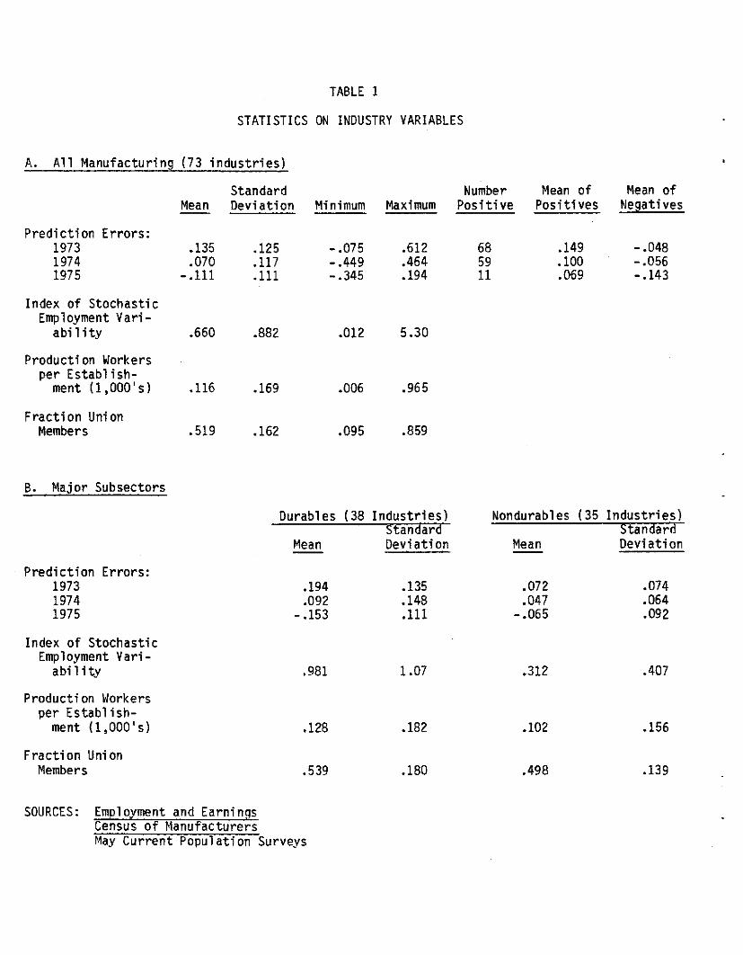
TABLE 1

STATISTICS ON INDUSTRY VARIABLES

A. All Manufacturing (73 industries)

Standard Number Mean of Mean ofMean Deviation Minimum Maximum Positi ve Positives Negatives

Prediction Errors:1973 .135 .125 -.075 .612 68 .149 -.0481974 .070 .117 -.449 .464 59 .100 - .0561975 - .111 .111 -.345 .194 11 .069 -.143

Index of StochasticEmployment Vari-

abil ity .660 .882 .012 5.30

Production Workersper Establish-

ment (l ,000' s) .116 .169 .006 .965

Fracti on Uni onMembers .519 .162 .095 .859

B. Major Subsectors

Durables (38 Industries) Nondurables (35 Industri es)Standard Standard

Mean Deviation Mean Deviation

Prediction Errors:1973 .194 .135 .072 .0741974 .092 .148 .047 .0641975 -.153 .111 -.065 .092

Index of StochasticEmployment Vari-

ability .981 1.07 .312 .407

Production Workersper Establ ish-

ment (l ,000' s) .128 .182 .102 .156

Fracti on Uni onMembers .539 .180 .498 .139

SOURCES: Employment and EarningsCensus of ManufacturersMay Current Population Surveys

TABLE 2

STATISTICS ON INDUSTRY VARIABLES AFTER ATTACHMENT TO CPS RECORDS

•A. Nonunion Workers

Standard Percent Mean of Mean ofMean Deviation Positive Positives Negati ves

Prediction Errors:1973 .165 .129 95 .176 -.0521974 .071 .114 78 .106 - .0561975 -.137 .108 11 .063 -.163

Index of StochasticEmployment Variability .665 .856

Production Workers perEstablishment (l,OOO's) .085 .122

Fraction Union Members(for industry) .484 .151

B. Uni on Workers

Predi cti on Errors:1973 .151 .122 95 .162 -.0451974 .077 .105 78 .108 - .0281975 -.125 .105 12 .060 -.152

Index of StochasticEmployment Variability .728 .785

Production Workers perEstablishment (l,OOO's) .168 .239

Fraction Union Members(for industry) .613 .155

SOURCES: Employment and EarningsCensus of ManufacturersMay Current Population Surveys

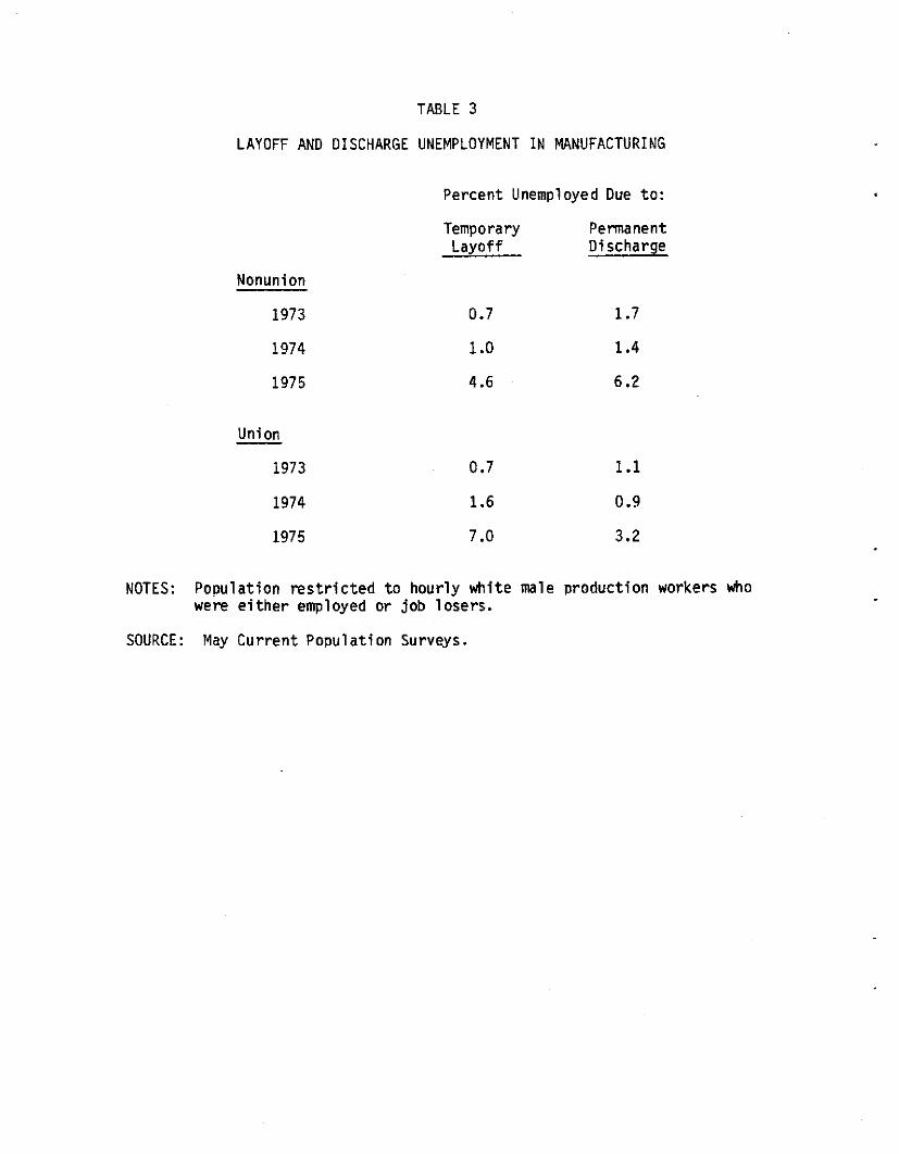
TABLE 3

LAYOFF AND DISCHARGE UNEMPLOYMENT IN MANUFACTURING

Percent Unemployed Due to:

Nonunion

1973

1974

1975

Union

1973

1974

1975

TemporaryLayoff

0.7

1.0

4.6

0.7

1.6

7.0

PermanentDischarge

1.7

1.4

6.2

1.1

0.9

3.2

NOTES: Population restricted to hourly white male production workers whowere either employed or job losers.

SOURCE: May Current Population Surveys.

TABLE 4

EXCESS HOURS IN MANUFACTURING

Standard Percent Mean of Percent Mean ofMean Deviation Positive Positives Negative Negati ves

Nonunion

1973 1.51 14.1 23.0 18.7 13.2 -21.1

1974 0.18 14.2 19.4 17.4 13.5 -23.7

1975 0.34 14.5 17.6 19.8 13.5 -23.3

Union

1973 2.87 15.2 25.3 21.1 10.9 -22.7

1974 2.04 13.7 20.8 20.7 10.5 -21.6

1975 0.02 13.0 14.2 20.0 13.2 -21.6

NOTES: A11 fi gu res are percentages. Population restricted to white male hourly productionworkers.

SOURCE: May Current Population Surveys.

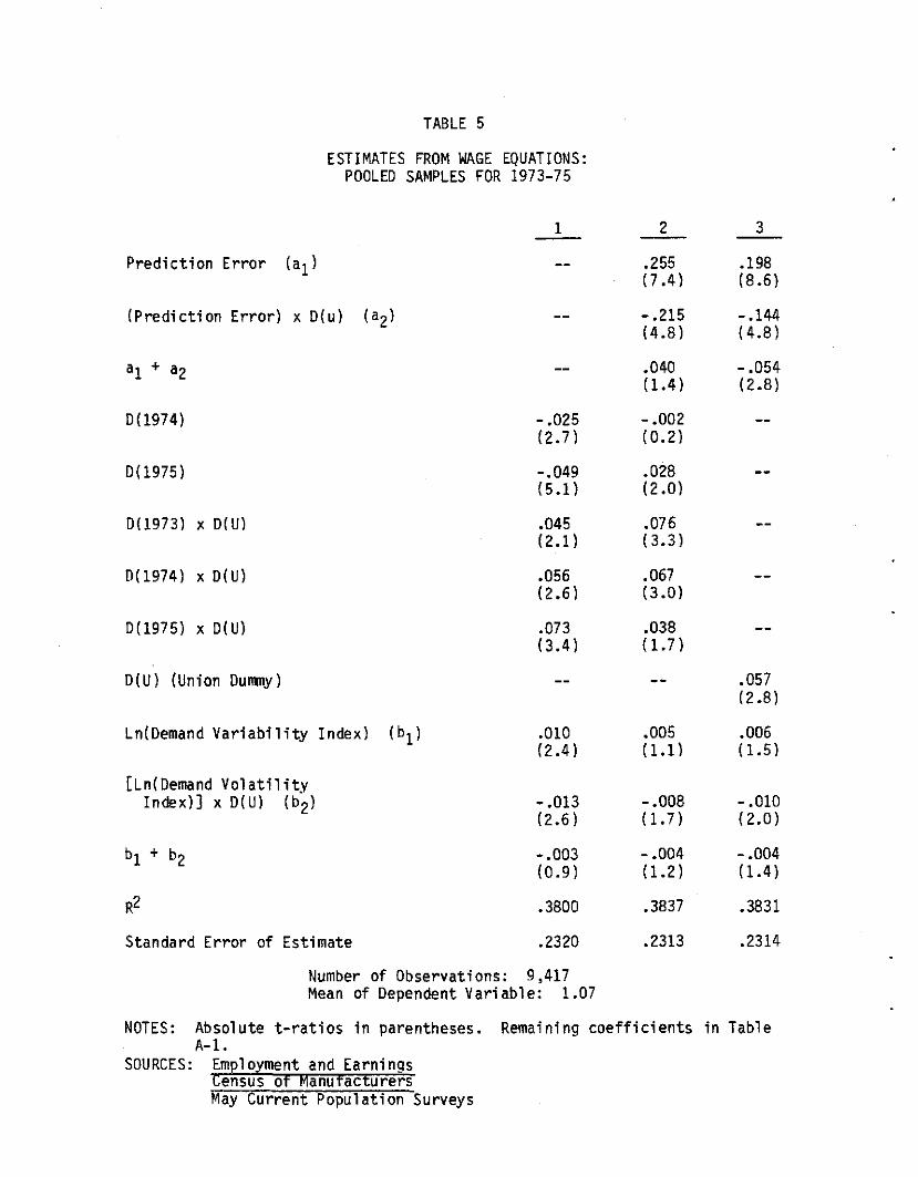
TABLE 5

ESTIMATES FROM WAGE EQUATIONS:POOLED SAMPLES FOR 1973-75

1

Prediction Error (a1)

(Prediction Error) x DIu) (a2)

0(1974)

0(1975)

0(1973) x OW)

0(1974) x DIU)

0(1975) x OW)

OW) (Union OUIl1llY)

Ln(Oemand Variability Index) (b1)

[Ln{Oemand VolatilityIndex)] x O(U) (b2)

Standard Error of Estimate

-.025(2.71

-.049(5.1)

.045(2.1)

.056(2.6)

.073(3.4)

.010(2.4)

-.013(2.6 )

-.003(0.9)

.3800

.2320

Number of Observations: 9,417Mean of Dependent Variable: 1.07

NOTES: Absolute t-ratios in parentheses. Remaining coefficients in TableA-I.

SOURCES: Employment and EarningsCensus of ManufacturersMay Current Population Surveys

TABLE 6

ESTIMATES OF COEFFICIENTS OFPREOICTION ERROR IN WAGE EQUATIONS:

SEPARATE SAMPLES FROM 1973-75

1973

Prediction Error (a1)

(Prediction Error) x D(U) (a2)

R2

Partial R2 (both variables)

Standard Error of Estimate

Mean of Dependent Variable

Number of Observations

NOTES: Absolute t-ratios in parentheses.

SOURCES: Same as Table 5

.295(4.2)

-.250(2.7)

.045(0.7)

.3679

.0056

.2331

1.10

3,247

1974 1975

.272 .418(4.5) (5.6)

-.174 -.301(2.1) (3.2)

.098 .117(1.8 ) (2.0)

.3940 .3953

.0074 .0118

.2264 .2344

1.07 1.06

3,177 2,993

TABLE 7

REGRESSION COEFFICIENTS FOR COMPAP.ING WAGE RESPONSEIN DIFFERENT INDUSTRY ENVIRONr1ENTSa

Prediction Error .221(5.3)

(Prediction Error) x O(U) -.195(3.6)

(Prediction Error) x (% Uni on) -.014(0.1)

(Predi cti on Error) x (% Uni on) x OW) .074(0.4)

(Prediction Error) x PWEb -.567(2.1)

(Predicti on Error) x PWE x O( U) .318(1.0 )

(Prediction Error) x Varc .015(0.8)

(Predi cti on Error) x Var x D(U) .014(0.6)

NOTES: aThe equation also contained all variables reported in the equati onreported in column 3 of Table 5 and Table A-I.

bpWE is production workers per establishment.

cVar is the measure of employment variability.

SOURCES: Same as Table 5

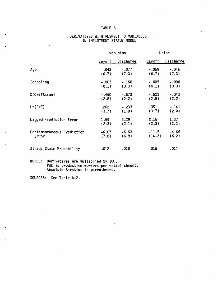
TABLE 8

DERIVATIVES WITH RESPECT TO VARIABLESIN EMPLOYMENT STATUS MODEL

Nonuni on Union

Layoff Discharge Layoff Discharge

Age -.043 - .077 -.059 -.046(6.7l (7.3) (6.7l (7.3)

Schooling -.003 - .160 -.005 -.096(O.ll (3.3) (O.ll (3.3 )

D(C raftsman) -.460 -.573 -.622 -.343(2.8 ) (2.2) (2.8) (2.2)

Ln(PWE} .262 -.233 .351 -.141(3.7) (1.9 ) (3.71 (2.0)

Lagged Prediction Error 1.59 2.29 2.15 1.37(2.3) (2.1l (2.3) (2.1)

Contemporaneous Prediction -6.07 -6.63 -11.5 -4.05Error (7.8 ) (6.9 ) {14.2 ) (6.2)

Steady State Probability .012 .018 .016 .011

NOTES: Derivatives are multiplied by 100.PWE is production workers per establishment.Absolute t-ratios in parentheses.

SOURCES: See Table A-2.

TABLE 9

DERIVATIVES WITH RESPECT TO VARIABLESIN HOURS ADJUSTMENT MODEL

Nonunion Union

Overtime Short time Overtime Short time

Age -.004 -1.81 -.001 -.161(0.1 ) (5.9) (0.3) (5.9)

Schooling .567 -.420 .540 -.369(2.9) (2.8) (2.9) (2.8)

D(Craftsman) .320 -1.41 .263 1.25(0.4) (1.9) (0.3) (1.9)

Ln(PWE} -1.28 -.849 -1.28 -.767(3.1) (2.5) (3.2 ) (2.6)

Lagged Prediction Error -15.8 4.47 -15.4 3.85(4.1) (1.4 ) (4.1 ) (1.4)

Contemporaneous 11.5 -1.59 24.4 -5.24Prediction Error (2.9) (0.5) (7.5) (2.1)

Steady State Probability .223 .129 .215 .113

NOTES: Derivatives are multiplied by 100.PWE is production workers per establishment.Absolute t-ratios in parentheses.

SOURCES: See Table A-3.

•

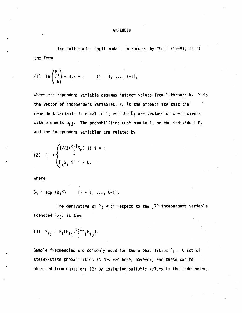
APPENDIX

The multinomial logit I11Odel. introduced by Theil (1969). is of

the form

(i=1.... ,k-1),

where the dependent variable assumes integer values from 1 through k. X is

the vector of independent variables. Pi is the probability that the

dependent variable is equal to i. and the Bi are vectors of coefficients

with elements bij' The probabilities I1llst sum to 1. so the individual Pi

and the independent variables are related by

•

(2 )

i = k

~/here

Si = exp (Bi X) (i = 1. "" k-ll.

The derivative of Pi with respect to the jth independent variable

(denoted Pi j) is then

(3 ) k-1= P.(b .. - : P.b .. )., 'J 1 ' 'J

Sample frequencies are commonly used for the probabilities Pi' A set of

steady-state probabilities is desired here. however. and these can be

obtained from equations (2) by assigning suitable values to the independent

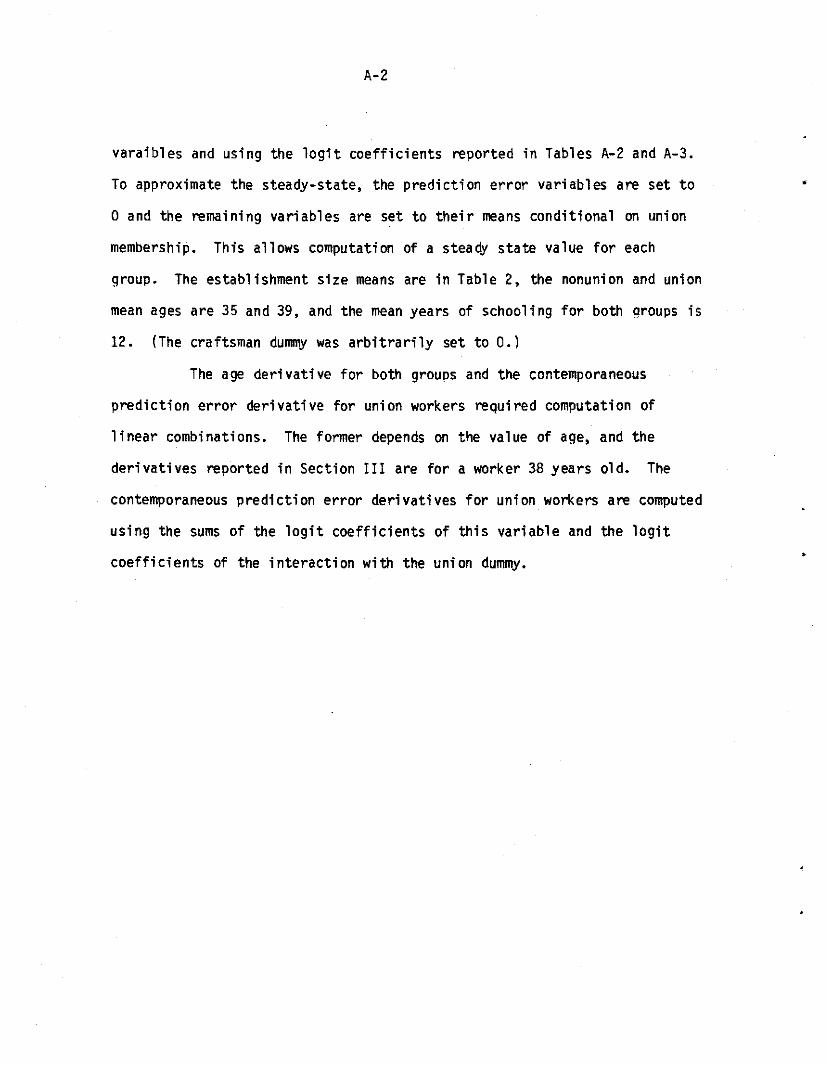
A-2

varaibles and using the logit coefficients reported in Tables A-2 and A-3.

To approximate the steady-state, the prediction error variables are set to

o and the remaining variables are set to their means conditional on union

membership. This allows computation of a steady state value for each

group. The establishment size means are in Table 2, the nonunion and union

mean ages are 35 and 39, and the mean years of schooling for both groups is

12. (The craftsman du~ was arbitrarily set to 0.1

The age derivative for both groups and the contemporaneous

prediction error derivative for union workers required computation of

linear combinations. The former depends on the value of age, and the

derivatives reported in Section III are for a worker 38 years old. The

contemporaneous prediction error derivatives for union workers are computed

using the sums of the logit coefficients of this variable and the logit

coefficients of the interaction with the union dummy.

•

•

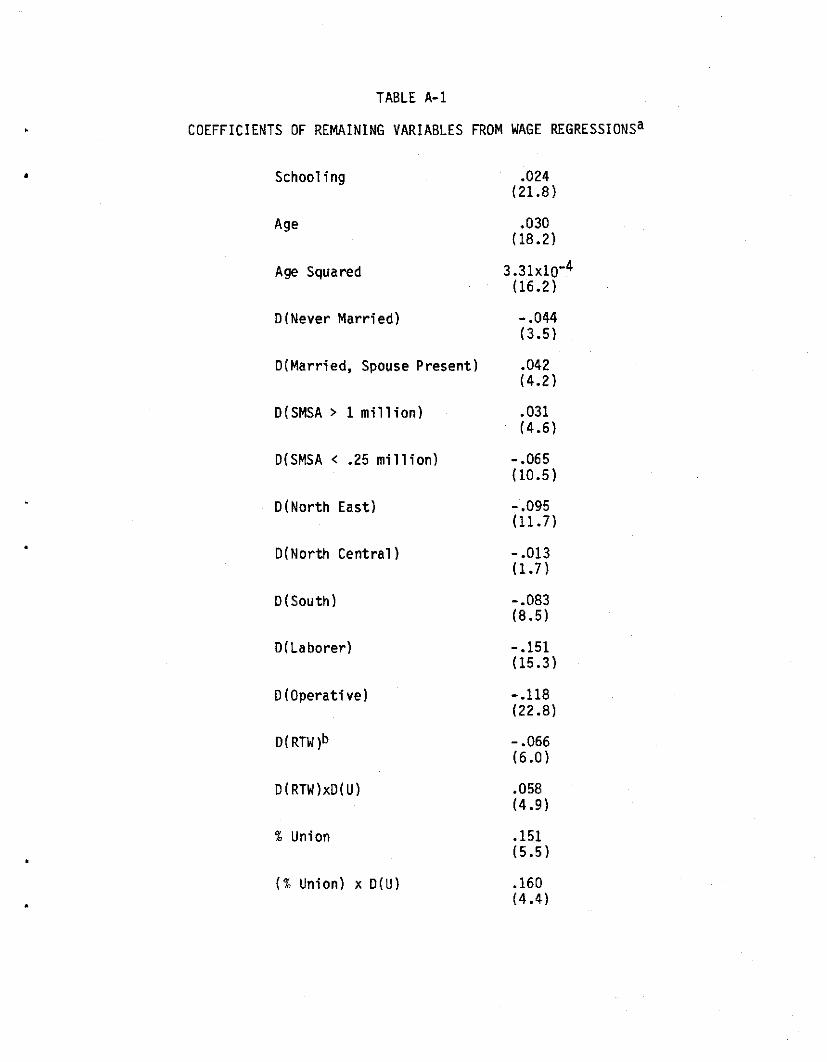
TABLE A-I

COEFFICIENTS OF REMAINING VARIABLES FROM WAGE REGRESSIONSa

•

•

•

Schooling

Age

Age Squared

D(Never Married)

D(Married. Spouse Present)

D(SMSA > 1 million)

D(SMSA < .25 million)

D(North East)

D(North Central)

D(South)

D(Laborer)

D(Operative)

D(RTW)b

D(RTW)xD(U)

X Union

(X Union) x D(U)

.024(21.8)

.030(18.2)

3.31x10-4(16.2)

-.044(3.5)

.042(4.2)

.031(4.6)

- .065(10.5 )

-.095(11.7)

-.013(1.7)

-.083(8.5)

-.151(15.3)

-.118(22.8)

-.066(6.0 )

.058(4.9)

.151(5.5)

.160(4.4)

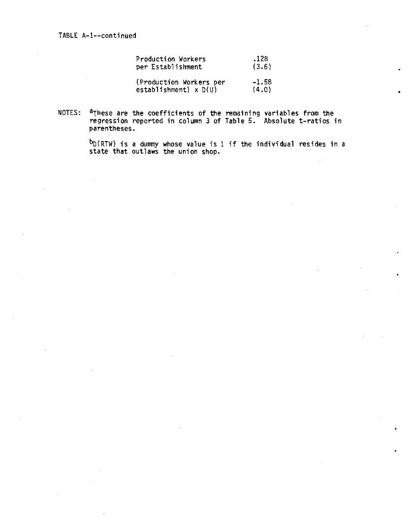
TABLE A-l--continued

Production Workersper Establishment

(Production Workers perestablishment) x D(U)

.128(3.6)

-1.58(4.0) •

NOTES: aThese are the coefficients of the remaining variables from theregression reported in column 3 of Table 5. Absolute t-ratios inparentheses.

bo(RTW) is a dummy whose value is 1 if the individual resides in astate that outlaws the union shop.

•

,

•

•

TABLE A-2

LOGIT COEFFICIENTS FOR EMPLOYMENT STATUS MODEL

Layoff Di scharge

Constant .184 1.20(2.3) 0.4 )

Age -.171 - .198(4.5 ) (4.9)

Age Squared 1.76x10-3 2.03x1D-3(3.6) (3.8)

Schooling -4.26x20-3 -.088(0.1) (3.3)

D(Craftsman) -.385 -.321(2.8) (2.2)

D{U) .294 -.315(1.9 ) (2.3)

Ln{PWE) .214 -.126(3.7) (1.9)

Lagged Prediction 1.34 1.28Error (2.3) (2.1)

Contemporaneous Predic- -5.08 -3.72tion Error (8.0) (7.0)

(Contemporaneous Predic- -2.03 - .110tion Error) x D{U) (2.5) (0.1)

Sample Proportions .026 .022

Number of Observations: 12,044Overall Chi Square: 598.5

NOTES: PWE is Production Workers per Establishment. Figures inparentheses are absolute t-ratios.

Chi Square

42.6

26.6

11.2

12.4

9.3

17.8

9.3

106.8

6.4

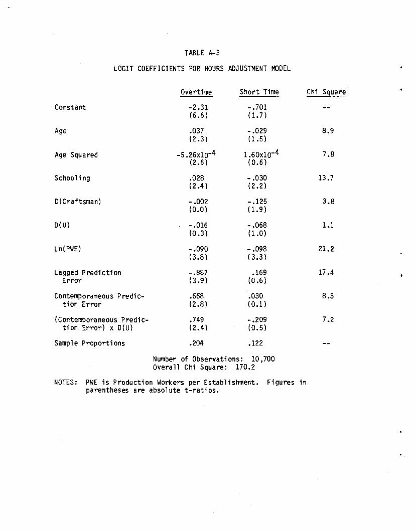
TABLE A-3

LOGIT COEFFICIENTS FOR HOURS ADJUSTMENT MODEL