W?s gj1D

POLICY RESEARCH WORKING PAPER 1970

Trade Liberalization and Although trade liberalizationhas been linked

Endogenous Growth in a econometrically and through

Small Open Economy casual empiricism to large

income increases, attempts to

quantify its impact in static

A Quantitative Assessment simulation models haveshown estimated gains. This

paper shows that when theThomas F. Rutherford endogenous dynamic effects

David G. Tarr of trade liberalization are built

into simulation models, the

estimated gains are indeed

very large. But complementary

regulatory, financial market,

and macroeconomic reforms

are important to realize the

largest gains.

The World Bank

Development Research Group

Trade HSeptember 1998

POLICY RESEARCH WORKING PAPER 1970

Summary findings

Rutherford and Tarr develop a numerical endogenous their central model, where the economy is assumed to begrowth model approximating an infinite horizon, which unable to borrow on international financial markets. Ifallows them to investigate the relationship between trade macroeconomic and financial reforms are in place thatliberalization and economic growth. would allow international borrowing, however, the same

Economic theory generally implies that trade tariff cut is estimated to result in a 37 percent increase inliberalization will improve economic growth, and the Hicksian equivalent variation. On the other hand, iftwo phenomena are positively correlated in empirical inefficient replacement taxes must be used in antests, but the connection is not well-substantiated in economy without the capacity to borrow internationally,numerical general equilibrium models. the gains would be reduced to 4.7 percent. Larger tariff

In the authors' model, an intermediate input affects cuts - typical of those in many developing countriesaggregate output through a Dixit-Stiglitz function. over the past 30 years - produce larger estimatedAdditional varieties provide the engine of growth in this welfare gains at least proportionate to the size of the cut.framework and the existence of this mechanism The authors apply the model to five developingmagnifies the welfare costs. In this model with lump sum countries and estimate the impact of the tariff changesrevenue replacement, reducing a tariff from 20 percent those countries plan to undertake as part of Uruguayto 10 percent produces a welfare increase (in terms of Round commitments. Because of the dynamic effects,Hicksian equivalent variation over the infinite horizon) estimated gains are considerably larger than those foundof 10.7 percent of the present value of consumption in in the literature on the impact of the Uruguay Round.

This paper - a product of Trade, Development Research Group - is part of a larger effort in the group to assess the impactof trade and investment on economic growth. The study was funded by the Bank's Research Support Budget under theresearch project "The Dynamic Impact of Trade Liberalization in Developing Countries" (RPO 681-40). Copies of thispaper are available free from the World Bank, 1818 H Street NW, Washington, DC 20433. Please contact Lili Tabada, roomMC3-333, telephone 202-473-6896, fax 202-522-1159, Internet address Itabada@worldbank.org. David Tarr may becontacted at dtarr@worldbank.org. September 1998. (49 pages)

The Policy Research Working Paper Series disseminates the findings of work in progress to encourage the exchange of ideas about

development issues. An objective of the series is to get the findings out quickly, even if the presentations are less than fully polished. Thepapers carry the names of the authors and should be cited accordingly. The findings, interpretations, and conclusions expressed in thispaper are entirely those of the authors. They do not necessarily represent the view of the World Bank, its Executive Directors, or thecountries they represent.

Produced by the Policy Research Dissemination Center

Trade Liberalization and Endogenous Growth

in a Small Open Economy: A Quantitative Assessment

by

Thomas F. Rutherford and David G. Tarr*

* Associate Professor, Department of Economics, University of Colorado; and Lead Economist,The World Bank. 'We would like to thank Richard Baldwin, Glenn Harrison and seminarparticipants at the April 1997 conference in Milan Italy on Technology Diffusion andDeveloping Countries for helpful comments. Research support was provided by the World Bankunder RPO No. 68140, "The Dynamic Impact of Trade Liberalization in Developing Countries."

1. Introduction

Intemational trade economists have typically argued that an opentrade regime is very important for

economic development. This view has been based partly on neoclassical trade theory, which generally finds

that a country improves its welfare from trade liberalization, partly on casual empirical observation that

countries which remain highly protected for long periods of time appear to suffer significantly and perhaps

cumulatively, and partly on systematic empirical work that also finds trade liberalization beneficial to welfan

and growth (e.g., Sachs and Warner, 1995).') What has been troubling is that the numerical modeling

estimates of the impact of trade liberalization have generally found that trade liberalization increases the

welfare of a country by only about one-half to one percent of GDP, gains which are very small in relation

to the paradigm.2' For many years authors have claimed that the welfare gains from trade liberalization wou!d

be much larger if the dynamic impact of trade liberalizationwere taken into account, but heretofore no such

models have been developed.3 )

')Of course, all aspects of the paradigm that trade liberalization leads to faster growth have been subject to criticism.For example, Rodrik (1992) has developed models in which trade liberalization is immiserizing, and causality hasbeen questioned in the Sachs and Warner results.

')See, for example, de Melo and Tarr (1990; 1992; 1993); Harrison, Rutherford and Tarr (1993; 1997a; 1997b); Morkreand Tarr (1980; 1995); and Tarr and Morkre (1984). The consistently small estimated gains in constant returns to scalemodels came to be known as "the Harberger constant." While some estimates with increasing returns to scale models(such as Harris, 1984) have been larger (up to 10 percent of GDP), these estimates have been more controversial, oftenbased on regime switching (see Harrison, Jones et al., 1993; and Harrison, Rutherford and Tarr, 1997a). In our view,the results are less than convincing for a strong version of the paradigm.

3'Moreover, we have shown, see Rutherford and Tarr (1997), that a comparative static model may be a closeapproximation to the annual welfare gains from trade liberalization in a dynamic model, if the dynamic model issimply Ramsey based, i.e., if there is no endogenous growth.

Some numerical general equilibrium modelers have produced comparative "steady state" estimates of the welfaregains which are two to four times the comparative static estimates of their models (e.g., Harrison, Rutherford andTarr, 1996, 1997; Francois, McDonald and Nordstom, 1996; and Baldwin, Francois and Portes, 1997). These aremulti-sector quantifications of the Baldwin (1989) 'medium term growth bonus," which hold the rental rate oncapital constant and allow the capital stock to vary. Harrison, Rutherford and Tarr (1996; 1997a) and Rodrik (1997)have explained, however, that these estimates overestimate the gains from trade liberalization in a Ramsey typemodel because they fail to adjust for the foregone consumption cost of achieving the higher capital stock.

-1-

With the development of endogenous growth theory (for example, Romer (1990), Romerand Rivera-

Batiz (1991), Grossman and Helpman (1991) and Segerstrom, Anant and Dinopoulos (1990)) a clear

theoretical link has been provided from trade liberalization to economic growth. Due to the complexity of

the models, however, the theoretical literature has necessarily focused on a comparison of the steady-state

growth paths, and been based on rather aggregated models. Since two policies that achieve the same steady-

state growth path could have very different welfare consequences, it is important to develop models that

derive the dynamic adjustment path and evaluate the welfare effect.

In this paper we develop a dynamic small open economy model defined over a 54 year horizon, frnm

1997 to 2050 with terminal constraints which approximate an infinite horizon. There are two sectors Xand

Y. The Y sector produces goods for domestic and export markets under constant returns to scale (CRTS).

Inputs into Yare labor and a pure intermediate goodX. The good Xis produced by both foreign and domestic

firms under the large group monopolistic competition assumption and increasing returns to scale (IRTS).4)

We employ the by now standard assumption that inputs ofXaffect the production of Yaccording to

a Dixit-Stiglitz function. This means that additional varieties of X reduce the cost of producing Y. Firms in

the IRTS sector must incur a once and for all fixed cost of a "blueprint" in order to introduce a new product;

and firms also incur a fixed cost in any period in which they operate. Domestic firms use relatively more

local inputs and relatively less imported inputs. Product development costs are lower for foreign firms under

the assumption that in relation to the size of the domestic market there is an infinite stock of varieties of

Nonetheless, the estimates for Hicksian equivalent variation remain less than five percent of GDP, except for theBaldwin, Francois and Portes paper; and Rodrik (1997) has estimated that after adjusting for the foregoneconsumption cost of investment, the estimated equivalent variation in the Baldwin, Francois and Porter paper wouldalso be less than five percent.

')Our analysis can be viewed as an extension of Ethier (1982) and Markusen (1989, 1991). Markusen investigatedthe implications of the substantial trade in imported intermediate inputs using static and two period models. Aprevious model of ours, Rutherford and Tarr (1996), also employed an Ethier-Dixit-Stiglitz framework to evaluatethe impact of trade liberalization. In that paper, however, the growth rate was not affected endogenously, so theadditional welfare gains from the variety effect were derived from transitional dynamics.

-2-

products on international markets; thus, their development costs represent solely the cost of adapting and

introducing a Product from the international market to the domestic economy. All agents in the model,

including firms in the IRTS sector, optimize over the infinite horizon with perfect foresight apart from

unanticipated policy changes.

In our central model, the country cannot borrow on international capital markets, so that the value

of imports must be covered by exports in each period of the model. We investigate the impact of allowing

capital flows in the sensitivity analysis.

The onl-v tax distortion in the economy in the benchmark data set is a twenty percent tariff on

imports. We first construct a steady state growthpath with which we can compare results of counterfactual

experiments. We then reduce the tariff to ten percent and compare all variables to their values in the

benchmark steady-state.

We construct a series of counterfactual scenarios to determine the sensitivityof the results to tax, macro and

financial policies, as well as to different tariff cuts and parameter specification. We evaluate the welfare

consequences of a change in policies, i.e., we report the Hicksian equivalent variationfor the infinitely-lived

representative agent.

Some of our mnost important results are as follows: with lump sum revenue replacement,

reducing a tariff from 20% to 10% produces a welfare increase (in terms of Hicksian equivalent

variation over the infinite horizon) of 10.7 percent of the present value of consumption in our central

model. We investigated the sensitivity of our results to all of the key parameters in the model and

found that the welfare estimates for the same tariff cuts ranged up to 37 percent with capital flows,

and down to 4.7 percent with inefficient replacement taxes. Doubling or quadrupling the size of the

tariff cuts, which would characterized the experience of many developing countries in the past 30

years, resulted in estimates of the welfare gains that were at least twice or four times, respectively,

-3-

the size of the cut. We applied the model to five developing countries and estimated the impact of the tarif

changes which they plan to undertake as part of their Uruguay Round commitments. Our estimatedgains are

large in relation to the literature estimates of the impact of the Uruguay Round.

Our results illustrate the crucial importance of complementary reforms to fully realize the potential

gains from the trade reform. Notably, with the ability to access international capital markets, the gains are

more than doubled. Moreover, use of inefficient replacement taxes will significantlyreduce the gains. These

combined results show that complementary macroeconomic, regulatory, and financial market reforms to

allow capital flows and efficient alternate tax collection are crucial to realize the pDtentially large gains from

trade liberalization.

Large welfare gains in the model arise because the economy benefits from increased varieties of

foreign X in the short run, and increased varieties of domesticX after several years. In order to assess the

importance of variety gains, we perform the tariff reform in a constant returns to scale, perfect competition

Ramsey model; then additional varieties do not increase total factorproductivity. In this model the Harberger

constant reemerges, as welfare gains are about 0.5 percent of the present value of consumption.

We apply our model to datasets for five countries: Argentina, Brazil, Korea, Malaysiaand Thailand,

and assess the effects on these economies of the tariff changes they agreed as part of their Uruguay Round

commitments. The relatively large welfare gains that we estimate for these five countries relative to the

literature estimates ofthe gains from the Uruguay Round for these countries, suggest that the large welfare

gains in our stylized model are not based on implausible parameter values.

Although estimates of equivalent variation have been widely seen as too small, some may question

whether our estimates are too large. To put these numbers in perspective, in appendix A we have

analytically derived the relationship between a permanent increase in the steady state growth rate and

equivalent variation. A welfare gain of between 10 and 35 percent of consumption corresponds to a

permanent increase in the growth rate of between 0.4 and I percent. A policy induced change in the growth

-4-

rate of this magnitude is quite plausible in the context of the actual long term per capita growth rates overthe

25-30 year period beginning in 1962. The highest average long term annual growth rates are for the four

"East Asian tigers," with rates over 6 percent (Korea at 6.7 percent is the highest). At the other extreme theie

are 17 countries, largely in Africa, with negative growth rates, three of which are less than negative 2

percent. The average per capita growth rate for developing (developed) countries as a whole is 1.6 (2.9)

percent with a standard deviation of the growth rate of 2 (1).5)

Sachs and Warner (1995) maintain that this large range and standard deviation of the growth rates

across developing countries is explained in large part by trade liberalizatbn. Based on cross-country growth

regressions, they estimate that open economies have grown about 2.45 percent faster than clcsed economies,

with even greater differences for open versus closed economies among developing countries. They note that

trade liberalization is often accompanied by macro stabilization and other market reforms, and their open

economy variable can be picking up these other effects as well.6 ) But they argue that trade liberalization is

the sine qua non of the overall reform process, because other interventions such as state subsidies often are

unsustainable in an open economy. While, like Sachs and Warner, our results show that trade liberalization

can have an important impact on growth, we also find that the benefits of trade liberalization can be dissipatad

without complementary reforms in the macroeconomic, financial and tax areas.

These econometric estimates suggest that our estimate of equivalent variation, which corresponds

in our central model to a growth rate change of 0.4 percent, may still be too small. But larger tariff changes

5)These estimates are taken from Pritchett (1997), who performed the calculations based on the Summers and Heston(1991) data.

6OBecause trade policy may be endogenous, some have criticized the Sachs and Warner OLS estimates as sufferingfrom simultaneity bias. Ann Harrison and Dani Rodrik (1997) have provided preliminary estimates, however, thatshow that the impact of trade liberalization on growth is even larger when the simultaneity bias is taken intoaccount; in particular, a ten percent reduction in the tariff as we have simulated above, is estimated to increase thegrowth rate by considerably more than our estimate of 0.3 percent. In addition, they show that the black marketpremium plays an equally important role as tariff reduction. Although Sachs and Warner take the black marketpremium as part of their openness measure, Harrison and Rodrik separate it and prefer to think of it as a proxy formacro stabilization.

-5-

than our ten percent cut produce larger welfare gains and correspond to higher changes in the growth rates.

On the other hand, Young (1995) has estimated that the majority of the growth amorg the four East

Asian tigers is explained by factor accumulation, not increases in total factor productivity. But even Young

has found that average annual total factor productivity growth was equal to 1.7 percent in South Korea, 2.1

percent for Taiwan and 2.3 percent for Hong Kong. Only Singapore had virtually zero growth in total factor

productivity according to Young's estimates. Using Young's data,) however, but correcting for a bias in the

estimation procedure, Rodriguez-Clare (1997) estimates that a much larger share (almost 60 percent ) of the

growth among these four countries is due to an increase in TFP. We ccnclude that a detailed examination of

the East Asian tigers leaves a sufficient role for policy in explaining growth that our equivalent variation

estimates are not excessive.

Since our model employs the Chamberlinian large group assumption, the markup over fixed costs

remains unchanged, so there are no rationalization gains. Thus, these calculations show that the Ethier-Dixit

Stiglitz characterization of production, where additional varieties lowers costs, is sufficient to generate the

large welfare gains and increase in per-capita income. We have also developed a model in which there are

positive spillovers from additional foreign varieties on the costs of introducing new domestic varieties.

Although the domestic industry recovers more rapidly, the welfare gains are mt significantly affected, since

additional domestic varieties come largely at the expense of foreign varieties. Since the existence of

spillovers is somewhat controversial, the robustness of our results with respect to spillovers provicbs support

for the variety-trade liberalization paradigm.

The remainder of this paper is organized as follows. Section 2 outlines essential features of our

model. Section 3 presents results and sensitivity analysis with respect to model structure. The application

7)For Singapore, Rodriguez-Clare corrected for inconsistencies in the data.

-6-

of the model to the Uruguay Round commitments of five developing countries is presented in Section 5.

Section 6 concludes. Appendix A provides further details on welfare calculations over an infinite horizon,

relating changes in the economic growth rate to infinite-horizon welfare and then show how we apply these

results to approximate infinite horizon welfare. Appendix B describes the stylized benchmark data set and

model calibration.

2. Model Formulation

We consider a two sector economy. The Y sector produces exports and final goods for the domestic

market under constant returns to scale (CRTS) and perfect competiticn. The X sector which is composed of

both domestic and foreign firms produces intermediate goods under increasing returns to scale (IRTS) and

imperfect competition with a Dixit-Stiglitz representation of the impact ofincreases in the number of products

on total factor productivity. Markups on goods in the IRTS sector are based on the Chamberlinian large

group assumption--that is, the elasticity of demand facing the representative firm is equal to the compensatel

elasticity of substitution between varieties. Final demand arises from an infinitely-lived epresentative agent

who is at the margin indifferent between an additional unit of consumption and an additional unit of

investment. In this section we outline the key features of the model in terms of the objectives and constraint

facing various agents.

2.1 Consumer Behavior

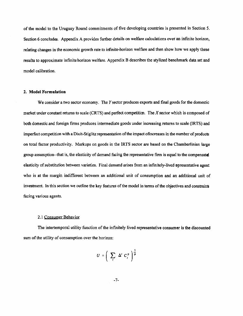
The intertemporal utility function of the infinitely lived representative consumer is the discounted

sum of the utility of consumption over the horizon:

u = ( E A' Cf P

-7-

In this equation the parameter p controls the intertemporal elasticity of substitutioti) and A is the single

period discount factor. Aggregate consumption in a given period (Q is a Cobb-Douglas aggregate of

consumption of domestic and imported final goods:

C =CD D CM Dt I f

We assume that imported final goods cannot be produced in the home market, due to technical

limitations of the domestic final goods sector. The agent's intertemporal and within-period consumption

decisions are weakly separable. Thus, the typical static first order condition applies on consumption decisions

within a time period, given a decision on how much b spend on consumption in any period. In the standard

manner, the intertemporal decision is based on the maximization of the utility function subject to the

constraint that the present value of consumption equals the present value of income:

max U = ( E A CD, CM t" P)p

s.t.

(1 + c) ( P t CD,t s j PM CM) = WI L + II

In this expression, all prices are defined in present value terms, discounted to period 0 (=1997). The

right side of the constraint, which is the present value of income, includes the present value of wage incomeO

together with profits from existing capital stocks and patents. T is the consumption tax, discussed below.

In a steady-state equilibrium, there are no pure profits, but along an adjustment path moving to a new steady

state there may be returns associated with existing capital and markups over marginal cost. In other words,

S) The intertemporal elasticity of substitution (T = 1/l-p- See table I for the assumed values of elasticities indifferent sectors.

9) Note that population is fixed over the time horizon. Economic growth results solely from productivityimprovements due to the accumulation of varieties, and the real wage increases over time relative to the prices ofdomestic output and imports.

-8-

pure profits and losses are only associated with current (extant) firms. All firms formedduring the model

horizon earn zero economic profit.

2.2 Government Revenue and Expenditure

The government provides public goods and services at an exogenous level through the infinite

horizon. While we presume that these goods are provided because they generate net benefits for the

representative consumer, we do not formally model the impactof public provision on consumer well-being.

Instead, we account for the cost of providing public sector services through the imposition of an equal-yield

constraint asserting that any change in tariff rates must be compensated by a permanent change in one of

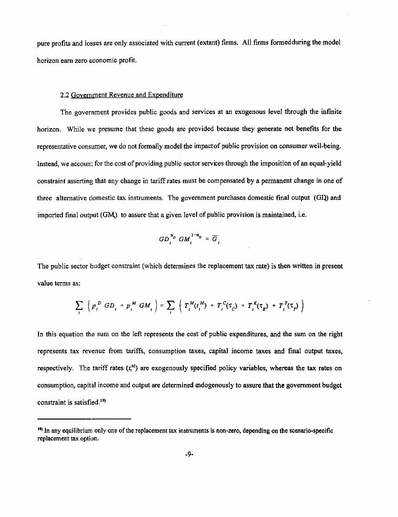
three alternative domestic tax instruments. The government purchases domestic final output (GD) and

imported final output (GM,) to assure that a given level of public provision is maintained, i.e.

GDD GM 1 GI

The public sector budget constraint (which determines the replacement tax rate) is then written in present

value terms as:

(p,D GD, + p,M GM,) = E ( T,M(ttM) + T,C(Tc) + T,K(CK) + T7Y(rY) )

In this equation the sum on the left represents the cost of public expenditures, and the sum on the right

represents tax revenue from tariffs, consumption taxes, capital income taxes and final output taxes,

respectively. The tariff rates (tQM) are exogenously specified policy variables, whereas the tax rates on

consumption, capital income and output are determined endogenously to assure that the government budget

constraint is satisfied.10)

10) In any equilibrium only one of the replacement tax instruments is non-zero, depending on the scenario-specificreplacement tax option.

-9-

2.3 Sales and Production of the Final Good

Good Y is produced as differentiated products for sale in the domestic and international markets. TIB

shares of sales at home and abroad are determined by relative prices. This iseffectively an Armington-style

differentiation of products in the export market. A constant elasticity of transformation (CET) function

relates the composite output level in a given period to domestic andexport sales. Firms producing the final

good maximize profit subject to the constraint:

y f (DJ + (1-T1D) (-| f

_~~~~ E

In this equation parameters D and E are the base year (1997) levels of output to the domestic and export

markets, and lD is the baseline value share of domestic sales in total sales (the base year production level is

scaled to unity).

Production of the Y composite is associated with a nested production function based on inputs of

labor (L) and differentiated intermediate inputs (xi ). Given prices of intermediate goods and labor, the

aggregate production sector operates so to minimize the costs of producing a given output subject to the

constraint:

IN a/p i ND P NF a/pL- i= -I- x PDS X

In this function, the intermediate inputs and labor enter in a Cobb-Douglas aggregate with value

shares determined by base year demands. It is evident from the production function that we have firm level

rather than national product differentiation. Since costs of varieties can differby foreign or domestic origin,

at the second level, within the intermediate input (X) nest, we account for substitution between domestic and

foreign varieties according to a constant-elasticity-of-substitution aggregation. The inputs of intermediates

-10-

from domestic and foreign firms represent the effective supply of X from these firm types. The effective

supply of all typef firms is described by:

( \ iipIp 1-p

Xf -- 1 ( X = (nfxf )XiP = nf Xf f E {D,F}

in which Xjf = Xf (by symmetry) is output of a representative typef firm, Xf = nff x,f is the total output from

typeffirms. Holding total output from type f firms constant, effective supply from type f firms increases wih

,-p I

nf P = nf,_ which is the "variety effect multiplier." The multiplier increases with 17 and increases as o

decreases toward 1 ( a >1). (The second equation in this expression reflects our assumption of symmetric

firm structure.) We then may express the aggregate production function as:

Y Li-a nL + p P _p COP

Following Romer and others, we assume that the value share ofX in aggregate production is related

to the elasticity of substitution between varietiesso that a=p, which implies that the elasticity itself is definel

by the value share as a = I/(1 -a). Making this substitution, we have the following expression for aggregate

output:

Y = (n L)I a * + ( L)a ?

2.4 Market Clearance Conditions

Output ofthe good Ysupplied to the domestic market can be consumed or invested. Investment in

XD andXF sectors involve forgone consumption of domestic output. The market clearance for macro output

sold in the domestic market is given by:

-1l-

D~ = CD~ +GD + p'DBf+ tnt( +D X,)D,C,G, E t MDF), ( , ,n, ( a,

This equation states that domestic output is purchased by households (CD,), government (GD ) and firms.

In turn, each firm type has four sources of demand for domestic output: (i) inputs to blue-print design

(D Bf), (ii) inputs to physical capital formation (I,), (iii) recurring fixed costs (np cD) and (iv) variable

costs of production (n a D X ). Both firm types (domestic and foreign) are treated symmetricaly, althoughft p f

we adopt parameters reflecting a relatively larger share of domestic inputs for the domestic firm. Domestic

firms are assumed to make investmnents in plant and equipment, whereas foreign firns who generally import

all the key components invest solely in distribution facilities such as warehouses and transportation

equipment.

The corresponding supply-demand balance for imported goods is as follows:

Mt CM, + GM, + (f ft aft xft)

Thus, imports enter into final demand by consumers and government and intermediate demand by firms.

Imported inputs ( p Bf) are required to establish either a domestic or foreign firm and are also required

for the fixed costs of operation (n afM xf,).ft p

2.5 Capital Stock Evolution

In our model, capital is firm-specific following installatbn, and investment rates may fall to zero as

a consequence of unanticipated changes in policy parameters. Following a standard Solow growth model,

investment in period t produces a unit of additional capital in the following year which may be used for

production in the future. Physical capital stock depreciates at a constant geometric rate:

-12-

K =XK + f e {D,F}ft+1 ft if,

whereas the number of blueprints (=number of firms) of each type are permanently in the market after they

are produced:

nf =n +Bf, f e {D,F}

2.6 Firms and Production Varieties

In sector Xthere is a one to one correspondence between firms and product varieties. The production

of good X involves both fixed and variable costs. Variable costs include inputs of aggregate output (domestb

and imported) and capital. Fixed costs can have two components: (i) "overhead", a recurring fixed capital

cost which is incurred in every period that the firm operates, and (ii) "setup costs", a one time research and

development (or blueprint) cost that must be incurred in order to design and market a new product. The

relative importance of blueprint and overhead costs are different for domestic and foreign firms. We asume

that foreign firms sell products which have been designed abroad, so their setup costs represert only the cost

of adapting an existing design to the domestic market. We model the productbn of blueprints by both types

of firm through the input of domestic and imported aggregates in fixed proportion. We assume in the present

model that there is no international trade in blueprints. Hence domestic firms may notlicense designs but

must purchase resources to develop new products from scratch.

We assume that most of the costs for foreign firms selling inthe domestic market are associated with

capital services and imported goods. In this setting the foreign firm's fixed costs of production may be

interpreted as the cost of maintaining a distribution system within the country.

The model is deterministicand firms have perfect (point) expectations of future prices. Hence, a new

firms will enter at time t if and only if there are positive net quasi-rents. This happens when the present value

-13-

of markup revenue"') over marginal costs into the future is equal to or greater than the present value of the

fixed costs of operation, including fixed operating costs (for foreign and domestic firms) and the fixed costs

of product development (for domestic firms). It is possible to interpret this decision using Tobin's q theory

(see Baldwin and Forslid, 1996). The rate of investment in blueprints occurs to the point that the stock marke

value of the net income (i.e., the present value of net surplus) equals the replacement costs, namely the

marginal cost of a blueprint, since R&D is perfectly competitive.

The Dixit-Stiglitz production function for good Xis perfectly symmetric with respect to domestic ard

foreign firms, i.e, we have firm level product differentiation, with no brand ornational preferences. Varieties

of different vintages are equally preferred but differentiated. In this framework, all domestic firms that

operate sell the same quantity of outputand their varieties sell for the same markup-inclusive price. Likewis

all foreign firms which operate sell the same quantity at the same price. Domestic and foreign firms enter

symmetrically in the final goods production function so the derived demand for domestic and foreign

intermediates is symmetric; but they remain differentiated and their prices may therefore differ. Since foreigi

and domestic firms are treated differently regarding their cost structures, their prices usually differ.

Furthermore, we assume that any firm producing at time t produces the same quantity as all other

firms irrespective of vintage, but differing according to whether it is foreign or domestic. This implies that

the share of total output produced by firms of vintage v is equal to the share of vintage v firms in the total

number of firms. These life cycle assumptions impose a symmetric structure on the equilibrium which maka

it possible to account for the share of markup revenue available in any period received by firms of vintage

V.

Unlike our previous model in which we tracked the level of investment for all vintages through the

model horizon, in the present model we achieve a considerable simplification byintroducing a state variable

This may be called "operating surplus", "operating profit" or "Ricardian surplus" by different authors.

-14-

for each firm type which tracks the present value of future markup earnings. This effectively treats the

human capital embodied in blueprint designs in the same analytic framework as is conventionally applied to

physical capital fornation. The underlying logic in unchanged from the previous model - the free-entry

assumption assures zero profit over the infinite horizon, and the time path of future prices affect not only

investment activity but the decisions by firms to enter markets and undertake product development.

Optimization over the infinite horizon applies not only to consumers and competitive firms, but also to the

managers of monopolistically competitive firms.

Our model is one of a small open economy. In particular, we assume that the small open economy

has only a negligible impact on the number of varieties available on world markets, and the cost of blueprint

for foreign firms. In general, we observe that there are many more varieties of products available on world

markets than are available in the small open economies. Accordingly, we assume that the decision facing

foreign firms is how many of the products for which blueprints akeady exist can be profitably introduced in

the local economy. The cost of the blueprint is a much smaller component of the cost of production for

foreign firms than for domestic firms -- and a larger fraction of the fixed costs of operation are associated

with recurring fixed costs of selling in the domestic market.

In the next section we investigate the properties of our model using numerical methods in vhich we

calibrate coefficients of utility and production functions to a reference growth path. Inthe results that follow,

we have assumed baseline data corresponding to table 1. These input parameters are reconciled to produce

the benchmark social accounts shown in table 2. For details on the translation of input data to model

parameters, see Appendix B.

-15-

3. Model Results

We consider a 54 year model horizon, defined over the years 1997-2050. Initially there is only one

distortion in the economy: a twenty percent tariff on imports of both goodX, the pure intermediate good

produced under IRTS and monopolistic competition, as well as the final good, produced under CRTS. In

order to establish a point of reference we calibrate a model to a "benchmark" steady-state equilibrium. In our

central counterfactual scenarios, we reduce the tariff from 20% to 10% on an ad valorem (net) basis and

compare the results in all scenarios to the benchmark steady-state equilibrium with the initial tariff in place.

Unless otherwise indicated, all key variables are reported as a percentage of their values in the benchmark

steady-state equilibrium.

In table 3 we present six model variants or scenarios. In our central model, we assume there are no

spillovers from the entry of foreign firms and that the lost tariff revenue is replaced by a lump sum tax on

consumption. In our second model, we allow for spillover effects of the entry of foreign firms which reduce

the costs of developing blueprints by domestic firms. In the third model, we assume all sectors opeate under

constant returns to scale and perfect competition; then there is no productivity boost in the Y sector as a resut

of additional varieties of the X good.

In all of our models we impose an "equal yield constraint" regarding government revenue. Unless

otherwise stated, the reduction in tariff revenue if offset by a consumption tax. Given he absence of a labor-

leisure choice, this is equivalent to a lump sum tax. We examine the impact of employing a final output tax

or a tax on capital as the replacement tax in the fourth and fifth models presented in table 3.

In our central model and unless otherwise stated, we assume thatthe country has difficulty accessing

international capital markets. This may be because it has imposed rstrictions on financial flows, or because

macroeconomic conditions in the country are such that it can not attract international investors. We takea

polar version of this assumption and assume that the country faces a balance of trade constraint in each

-16-

period, i.e., the value of its exports must equal the value of its imports (both a world prices) in each period.

We relax this constraint in the sixth model, where we allow the home country to borrow on international

capital markets provided any borrowing is repaid within the model horizon. Then,the present value of exports

must equal the present value of imports over the model horizon.

In all scenarios we present the Hicksian equivalent variation (EV). The EV is based on the

intertemporal utility function optimized over the 54 year model horizon, with an approximation for the

infinite horizon. We present EV in percentage terms, where the denominator is the present value of

benchmark consumption over the infinite horizon. In the figures, we present the 54 year time path for key

variables in percentage change relative to the steady-state. The variables we report are as follows: Figure 1:

Final Consumption, composite of domestic and imported final goods Figure 2: Real Exchange Rate; Figure

3: Rental Rate on Capital; Figure 4 and 5: Number of Domestic and Foreign Firms, respectively; Figure 6:

Consumption Paths for Alternate Replacement Taxes.

3.1 Tariff Reduction with Central Assumptions

We first consider the scenario in which we cut all tariffs from 20% to 10%. In this scenario, Hicksiai

equivalent variation (EV) increases by 10.7 percent of the present value of consumption over the infinite

horizon.

What is driving these results is the following. The removal of the tariff on imported intermediates

results in an increase in the tariff ridden demand curve for imports and an increase in the price foreign firms

receive for their products. This increases the present value of quasi-rents for foreign firms. Entry by foreign

firms occurs in any period until the present value of the quasi-rents are driven down to the one time start up

costs of establishing a domestic presence for the foreign firm plus present value of the fixed costs of

operating the domestic subsidiary. After about 1O years, the number of foreign varieties stabilizes for the

duration of the model horizon at about 30% more than in the steady state. (See figure 5.) The increase in

-17-

imports, however, results in a substitution effect that reduces the demand for and price ofdomestic varieties;

this shuts down investment and firm creation for the domestic variety for a period of about 6 years.

Although the increase in foreign varieties has the impact of decreasing the demand for domestic

varieties of the intertnediate good X, the domestic industry eventually stabilizes after 8 years rather than

progressively going into demise. (See figure 4.) The principal reason for this is that the marginal productivity

of domestic X in Y production increases as use of domestic X in Y declines. The entire labor force is

employed in the production of Y, and it is not possible to reduce labor usage applied to domestic Xwithout

also reducing labor usage in imported X. Thus, as domestic X declines due to substitution toward cheaper

imported X, its marginal product increases to eventually arrest the further decline of the dometic X industry.

The transitional dynamics of the model in the early years are dominated by theincrease in the number

of foreign firms. The increase in the number of firms has an immediate impact on theproductivity in the final

good sector inducing output of the final good sector to increase in the first year. This immediate increase in

productivity and output of the final goods sector allows the economy to satisfy two constraints painlessly:

(1) the economy is able to invest more in intermediate goods(it takes capital to produce the foreign variety)

without reducing consumption in the short run relative to the steady state. Although the economy facesa

Ramsey problem of determining the optimal tradeoff between consumption and investment, the tradeoff is

within the framework of an expanded choice set relative b the steady state. In fact, the economy consumes

about 7 percent more in the initial years compared with the benchmark steady state (see figure 1); and (2)

despite the period by period balance of trade constraint, the economy is able to import more foreign

intermediate varieties, without reducing its imports of final goods. The economy meets its balance of trade

constraint by exporting more of the final good. Thus, reducing the tariff does not result in any adjustment

costs in this model except for the losses that accrue to the specific capital owners in the domestic intermediat

goods sector. The surge in productivity results in both a 'level" effect and a growth effect regarding the

increase in consumption. The level effect can be observed by the jump in consumption in the first year. In

-18-

addition, however, due to an increase in the rental rate on capital (figure 3), the long run growth rate increases

from 2 to 2.1 percent.'2 )

3.2 Tariff Reduction with Spillovers

In this scenario, we cut the tariff on both final and intermediate inports from 20% to 10%, starting

in the initial period. Crucially, we allow an increase in the nunber of foreign firms to decrease the blueprint

costs for domestic firms, with a spillover elasticity equal to four percent. The equivalent variation of this

scenario is 10.9 percent of the present value of consumption, which differs by only a smal amount from the

10.7 percent for EV in the central model without spillovers.

The decrease in the tariff has the effect of increasing the number of foreign varieties, just as it does

in the central model. With spillovers, however, an increase in the number of foreign varieties has two

competing effects on investment in the domestic variety of X. On the one hand, as the number of foreign

varieties increases, the demand for the domestic variety decreases, so the quasi-rents available for domestic

firms decreases--decreasing the likelihood of domestic investment. On the other hand, the costs of domestic

blueprints decreases with the number of varieties--increasing the likelihood of investment. Inour formulation

of spillover effects, a 100 percent increase in the number of foreign varieties relative to the steady state,

reduces the blueprint costs of domestic firms by roughly 4 percent relative to the steady state blueprint costs

With these parameters, the spillover effect dominates after about 6 years, after which investnent h domestic

firms resumes. Relative to their steady state value, the number of domestic firms bottoms out at about 90

percent of their steady state value after about 7 years, and climbs to the benchmark steady state value by

'2) In this model the domestic and international rental rates on capital are decoupled, so a tariff reform produces apermanent increase in the domestic interest rate and a larger long-run increase in the growth rate. The domesticinterest rate is computed using the price of final consumption. This rate can temporarily depart from theinternational rental rate on capital in the model with perfect capital markets due to Armington differentiation ofdomestic and imported goods. In the long run, the domestic interest rate and the international rate convergeaymptotically.

-19-

2050.

It may appear puzzling that with spillovers, where the domestic industry has its costs reduced by

foreign varieties, the economy does not gain a significantly larger amount. The reason is that what is most

important to the welfare increase is the number of varieties rather than tin geographic source of them. With

spillovers, once the profitability of investment is restoredfor the domestic industry producing goodX, growth

of new foreign varieties falls-so there are more domestic firms and varieties, but fewer foreign varieties. TIC

loss of productivity due to the loss of foreign varieties almost fully offsets the gain in welfare due to the

increased number of domestic varieties.

3.3 Constant Returns to Scale (No Variety Multiplier)

In this model, we replace increasing returns to scale and imperfect competition in the intermediate

sector with constant returns to scale and perfect competition. Then only total output of the intermediate is

important (numbers of varieties are not counted), so there is no variety productivity effect. Although

consumers and decisions by investors optimize the consumption-capitd stock choice as in a Ramsey model,

there is no endogenous growth.

Equivalent variation for this scenario drops to 0.5 percent of the present value of consumption over

the infinite horizon. Without the variety multiplier, there is neither the initial "level" effect in consumption

nor the growth rate effect that obtained in our central and spillover models. Transitional dynamics are then

more painful, since in order to finance the additional investment in the earlier period, consumption falls in

the early years relative to the steady state. This result is similar to the results of Rutherford and Tarr (1997)

who showed that a Ramsey multisector model with constant returns to scale is insufficient to generate the

large welfare gains claimed for the trade liberalization paradigm .

3.4 Impact of Alternate Replacement Taxes

-20-

Except for the scenarios discussed in this subsection, we have employed a consumption tax as our

replacement tax. In the scenarios described here, we use two alternate taxes as the replacement tax for the

lost tariff revenue: a tax on output; and a tax on capital. The impact on the path of consumption, as a functicn

of the three replacement taxes, are presented in figure 10.

The curve labeled Consumption Tax is the same curve as in figure 1. Consumption increases to

between 7 and 12 percent of benchmark consumption during the model horizon. The consumption tax is a

Lump Sum distortionless tax in our model, but a tax on dormstic output introduces certain inefficiencies. In

particular, a domestic output tax discriminates against dometic output in favor of imports, and against final

output in favor of intermediate production. As a result of the relative inefficiency ofthe domestic output tax,

the path of consumption is cut by about 40-50 percent relative to the one with a tax on consumption and the

equivalent variation is reduced to a gain of 6.7 percent of the present value of consumption..

Finally, the tax on capital produces a consumption path that is inferior to the one with an cutput tax,

but preferable to the benchmark path with the tariff in place, i.e., the tax on capital is the most inefficient of

our three replacement taxes, but is better than a tariff in our model. In our model, the intermediate good X

uses capital intensively since only intermediate production uses capital as a primary input and only final

goods use labor as a primary input.'3 ) A tax on capital then discourages the introduction of new varieties

since it discourages the investment required for the introduction of new varieties of products and discourages

the production of intermediates relative to the production of final goods. The economy loses tie productivity

boost from the varieties and the gain in equivalent variation is less than only 4.7 percent of the value of

consumption. These results illustrate the importance of efficient tax replacement. With inappropriate

replacement tax mechanisms, the gains from trade liberalization can be drastically cut.

'3)Each good is used as an internediate input in production of the other good, and thus both goods use bothprimary factors of production indirectly.

-21-

3.5 Capital Flows

In this scenario, the tariff is reduced from 20% to 10%, but the country is assumed to be able to

borrow on international capital markets provided that the borrowing is repaid within the model horizon. Tha

the period-by-period balance of payments constraint is replaced by the constraint that the present value of

its exports less imports is zero over the model horizon, and all other assumptions in the central model

remained unchanged. In this scenario Hicksian equivalent variation (EV) is 37 percent of the present value

of benchmark consumption over the infinite horizon. There is an initial jump in consumption of about 23

percent, and relative to the steady state, the wage rate increases by about 110 percent by the year 2050.

Why is the increase in EV with capital flows more than three times the EV value without capital

flows? The decrease in the tariff implies that there is an incentive for new foregn firms to enter, as in the no

capital flows model. The ability of the country to borrow, however, allows the country to run trade deficits

and import much more in the periods immediately following tariff reduction. These additional imports are

used to finance the start up capital of new foreign firms and to pay for the additional imports of foreign

varieties. Foreign firms increase by almost 100 percent of their steady state value with capital flows by the

year 2003, as opposed to an increase of about 35 percent of their steady state value without capital flows. Tie

larger increase in foreign firms leads to a considerably larger increase in labor productivity and the wage rat

in the early years.

What is interesting is that there is a much larger increase in the number of domestic firmswith capital

flows-in fact, the number of domestic firms increases dramatically relative to the steady state value by the

end of the model horizon. This is explained by a real exchange rate effect. The economy finds it optimal to

run trade deficits in the early years of the model. These trade deficits finance additional inport varieties and

additional consumption in the early years."4 ) The capital inflows in the early years result in less real exchanW.

'4)The latter occurs because consumers optimize consumption over the model horizon subject to their lifetimeincome constraint or permanent income. With the ability to borrow on intemational capital markets, consumers can

-22-

rate depreciation in the early years of the model (in fact, they result in real exchange rate appreciation in the

first two years); but the capital outflows in the later years of the model result in a strong real exchange rate

depreciation in those years. (See figure 2.) The steeper real exchange rate depreciation with capital flows

in the years following 2020 (compared with central assumptions) raises the costs of importing foreign

varieties in those years, and shifts demand toward domestic varieties. Domestic agents, who fully anticipate

future real exchange rate movements, recognize profit opportunities and begin to invest by the year 2003.

Among the models we consider, it is perhaps ironic that the model with capital flows, where we see the

largest initial increase of foreign firms, ultimately leads to by far the strongest resurgence of domesic firms,

even compared to the model with spillovers.

3.5 Sensitivity Analysis

In table 4 we present the results of our sensitivity analysis for the key parameters in our model, and

we investigate the impact of different tariff changes. We present the Hicksian equivalent variation for each

scenario (with the approximation for the infinite horizon), and the growth rates calculated over three time

horizons: 1997-2010; 1997-2050; and 2049-2050, which is the projected growth rate into the infinite horizon

Except for the last three rows, in all scenarios the tariff rate is reduced from 20 to 10 percent.

As a point of reference, in row 0 we present the,results obtained with our central assumptions,

previously presented in row 1 of table 3. The result from row I illustrates that the larger the share of imported

in intermediate use (0), the larger the EV gains. The reason is that for a given ten percent cut in the tafiff, the

same proportional effect on the share of imports, generates more imported varieties, with the consequent

productivity boost, when this share is high. For the share of intermediates in final production (a), there are

offsetting effects: a higher share of intermediates in final production shotld increase the number of varieties

smooth consumption more easily.

-23-

because again the proportional change induced by a ten percent tariff cut should induce a larger increase in

the number of varieties; but the larger is a, the smaller is the variety multiplier for any number of varieties.

Thus, the impact of a change in this parameter on EV is ambiguous, and our two simulations presented in

rows 2 and 3 along with the central model show that EV as a function of a is not monotonic in the range of

our central elasticity values.

In the benchmark steady state, the rental rate on capital is 5 percent and thegrowth rate is 2 percent.

It is shown in appendix A that as these two rates approach each other, a given permanent increase in

consumption over the infinite horizon yields a larger EV. In rows 4 and 5, we illustrate the magnitude of the

change by varying each of these rates by one percent from the benchmark.

The results in row 6 indicate that, as is typical in comparative static models, themore elastic are the

substitution possibilities, the greater the gains. In particular, with a larger elasticity of transformation, the

economy is able to export more in response to a real exchange rate depreciation following tariff reduction,

which allows it to pay for more imports; and the additional intermediate imports provide a productivity b@st

through the additional varieties. The impact of this parameter is quite strong, as EV increases from 10.7 to

17.1 percent with a doubling of the elasticity of transformation.

Given that many developing countries in the past 30 years have started from protection levels well

above 20 percent and have implemented trade liberalizations considerably in excess of a ten percent tariff

cut, in rows 7, 8 and 9 we examine the impact of cutting the tariff from 2O percent to zero, from 40 percent

to 30 percent and from 40 percent to zero. For the results in rows 8 and 9, we generated a new baseline

steady state growth path with a 40 percent tariff in place. The results of rows 7 and 9 show that the gains are

very substantial for larger tariff cuts-the increase in EV from cutting the tariff from 40 percent to zero is moie

than 50 percent, which is more than double the gain of a cut from 20 percent to 0. Based on measurement

of Harberger triangles, comparative static models also produce the result that the gains increase more than

proportionately with the size of the tariff cut; but the result here is based on the fact that in our simulations

-24-

the number of varieties more tlhan doubles with a doubling of the tariff cut.

5. Application to the Uruguay Round Tariff Cuts of Five Developing Economies

In order to assess whether the large welfare results obtained above are dependent on possibly

unrealistic parameter values, we aply this model to five countries: Argentina, Brazil, Korea, Malaysia and

Thailand. We simulate the impact of the tariff cuts only on the intermediate products that these countries

agreed to as part of their Uruguay Round commitments. That is,we ignore the tariff cuts they made on final

products, as well as any liberalization in services.

For these countries., we employ the "GTAP" dataset (see Gelhar et al., 1997) and aggregate the

following GTAP sectors into our single intermediate goods sector: pulp and paper; chemicals, rubber and

plastics, non-metailic mineral products, primary ferrous metals, non-ferrous metals, fabricated metal

products, transport industries, machinery and equipment, other manufacturing products, and other services

(private). The resulting parameter values, including the tariff cuts are presented in table 5. Although all

countries have a share of intermediates over 60 percent, the share of imports in intermediates varies from 7

percent in Brazil to 71 percent in Malaysia. Tariff cuts on intermediates varies from 2 percent for Malaysia

to 8 percent for Brazil.

We examine the impact of these Uruguay Round tariff cuts in two models: first in our endogenous

growth model with central assumptions; and next in a constant returns to scale Ramsey model. In our central

model, the Hicksian equivalent variation increase ranges from 1.4 to 7.8 percent of the present value of

consumption over time. The largest value is in Thailand, which is theonly country of the five with a large

share of imported intermediates, and a relatively large tariff cut of seven percent. Argentina's low share of

imported intermrnediates and only five percent tariff cut explains its relatively low welfare gain.

These results are not intended to be a precise estimate of the gains from the Uruguay Round for these

economies (see Hlarrison, Rutherford and Tarr, 1 997a). Rather they suggest that the our large welfare gains

-25-

are not based on implausible parameter values. In the Ramsey model, the lack of variety induced productivity

increases results in quite small welfare increases, ranging from 0.1 percent in Korea and Malaysia to 0.4

percent in Thailand. Again, this indicates that estimated welfare gains are inthe range of the estimates from

competitive, static model.

5. Summary and Conclusions

This paper has investigated the effects of tariff liberalization in a small open economy in which

endogenous growth is linked to the introduction of new products by domestic or foreign firms. We have

developed a dynamic numerical model which allows us to trace out the dynamic adjustment path of all

variables and approximate the infinite-horizon welfare consequences of a change in policies. In our central

scenario, the tariff is cut from 20 percent to 10 percent, and we consider the impact both when the country

can access international capital markets and when it cannot.

We found that the welfare gain (Hicksian equivalentvariation) from tariff reform is 10.7 percent of

the present value of consumption in our central model,, a significant increase considering that the benchmak

tariff rate is only cut from 20 percent to 10 percent. We investigated the sensitivity of our results to all of

the key parameters in the model and found that the welfare estimates for the same briff cuts ranged up to 37

percent with capital flows, and down to 4.7 percent with inefficient replacement taxes. Larger tariff cuts,

which have characterized the experience of many developing countries in the past 30 years, resulted in

increases in the estimates of the welfare gains that were at least proportionate to the size of the cut.

We applied the model to five developing countries and estimated the impact of the tariff changes

which they plan to undertake as part of their Uruguay Round commitments. The gains of 0.7 percent to 7.8

percent that we estimate for these countries are large in relation to the comparative static or comparative

steady state estimates of the effects of the Uruguay Round for these countries.

Clearly these results support the paradigm that trade liberalization leads to significant income

-26-

increases, but they also illustrate the crucial importance of complementary reforms to fully realize the

potential gains from the trade reform. Notably, with the ability to access international capital markets, the

gains are more than doubled. Moreover, use of inefficient replacement taxes will significantly reduce the

gains. These combined results show that while there are indeed large gains possible from trade liberalizatioii

complementary macroeconomic, regulatory, and financial market reforms to allow capitalflows and efficient

alternate tax collection are crucial to realize the large gains.

-27-

References

Baldwin, Richard (1989), "The Growth Effects of 1992," Economic Policy, 0(9), October, 247-281.

Baldwin, Richard, Joseph Francois and Richard Portes (1997), "The Costs and Benefits of EasternEnlargement: the impact on the EU and central Europe," Economic Policy, April, 127-170.

Baldwin, Richard and Rikard Forslid (forthcoming), "Putting Growth Effects in CGE Models," in RichardBaldwin and Joseph Francois (eds.) Dynamic Issues in Applied Commercial Analysis, Cambridge:Cambridge University Press.

Crafts, Nicholas and Gianni Toniolo (1995), "Post-War Growth: An Overview," Discussion paper number1095, London: Centre for Economic Policy Research, January.

Dixit, A. and J. E. Stiglitz (1977), "Monopolistic Competition and Optimum Product Diversity," AmericanEconomic Review, 67, pp. 297-308.

Ethier, W. J. (1982), "National and International Returns to Scale in the Modem Theory of InternationalTrade," American Economic Review, 72, pp. 389-405.

Feenstra, Robert and James Markusen (1994), "Accounting for Growth with New Inputs," InternationalEconomic Review, 35 (1), pp. 429-447.

Francois, J. F. and C. R. Shiells (1993), "The Dynamic Effects of Trade Liberalization: A Survey," UnitedStates International Trade Commission Publication 2608, Washington, D. C.

Gehlhar, Mark; Gray, Denice; Hertel, Thomas W.; Huff, Karen; lanchovichina, Elena; McDonald, BradleyJ; McDougall, Robert; Tsigas, Marinos E., and Wigle, Randall (1997), "Overviewof the GTAP DataBase", in T.W. Hertel (ed.), Global Trade Analysis: Modeling and Applications, New York:Cambridge University Press.

Grossman, G. and E. Helpman (1991), Innovation and Growth in the Global Economy, MIT Press:Cambridge, MA.

Harris, Richard (1984), 'Applied General Equilibrium Analysis of Small Open Economies with ScaleEconomies and Imperfect Competition," American Economic Review, 74(5), December, 1016-1032.

Harrison, G. W., R. Jones. L. Kimbell, and R. Wigle, "How Robust Is Applied General EquilibriumAnalysis?",Journal ofPolicy Modeling, 15(1), 1993, 99-115.

Harrison, G. W., T. F. Rutherford, and D. G. Tarr (1993), "Trade Reform in the Partially LiberalizedEconomy of Turkey," The World Bank Economic Review, 7 (2), pp. 191-217.

Harrison, G. W., T. F. Rutherford, and D. G. Tarr (1996), "Increased Competition and Completion of theMarket in the European Union," Journal of Economic Integration, 11 (3), 332-36S.

-28-

Harrison, G. W., T. F. Rutherford, and D. G. Tarr (1997a), "Quantifying the Uruguay Round," EconomicJournal, 107, September, 1405-1430.

Harrison, G. W., T. F. Rutherford, and D. G. Tarr (1997b), "Economic Implications for Turkey of a CustomsUnion With the European Union," European Economic Review, 41, 861-870.

Keller, W. (1995), "Trade and the Transmission of Technology," Working Paper, Department of Economics,University of Wisconsin.

Keuschnigg, Christian and Wilhelm Kohler (1996), Economic Transition, Endogenous Innovation andCapital Accumulation," paper presented at the Centre for Economic Policy Research conferenceon Dynamic Issues in Applied Commercial Policy Analysis, January.

Markusen, J. R. (1991), "First Mover Advantages, Blocked Entry and the Economics of UnevenDevelopment," in E. Helpman and A. Razin (eds), International Trade and Trade Policy, CambridgeMA.: MIT Press.

Markusen, J. R. (1989), "Trade in Producer Services and Other Specialized Inputs,"American EconomicReview, 79, 85-95.

Melo, J. de and D. Tarr (1992), A General Equilibrium Analysis of US Foreign Trade Policy, CambridgeMA.: MIT Press.

Melo, J. de and D. Tarr (1990), "Welfare Costs of U.S. Quotas in Textiles, Steel and Autos," Review ofEconomics and Statistics, 72 (3), 489-497.

Melo, J. de and D. Tarr (1993), "Industrial Policy in the Presence of Wage Distortions: The Case of the USAuto and Steel Industries," International Economic Review, 34 (4), 833-851.

Mercenier, J. and P. Michel (1995), "Temporal Aggregation in a Multi-Sector Economy with EndogenousGrowth," Working Paper 554, Federal Reserve Bank of Minneapolis.

Mercenier, J. and P. Michel (1994), "Discrete time finite horizon approximation of optimal growth withsteady state invariance," Econometrica.

M. Morkre and David Tarr (1980), Effects of Restrictions on United States Imports: Five Case Studies andTheory, Washington, D.C.: Federal Trade Commission.

Morkre, M. and D. G. Tarr (1995), "Reforming Hungarian Agricultural Trade Policy: A QuantitativeEvaluation," Weltwirtschaftliches Archiv, pp. 106-131.

Roberts, Mark, Theresa Sullivan and James Tybout (1995), "What Makes Exports Boom? Evidence fromPlant-Level Data," The World Bank, mimeo.

Rodriguez-Clare, Andres (1997), "The Neoclassical Revival of Growth Economics: Has it Gone too Far?"Brookings 1997 Macroeconomics Annual.

-29-

Rodrik, Dani (1992 ), "The Limits of Trade Policy Reformn in Developing Countries," Journal of Economic

Perspectives, 6(1), Winter, 87-105.

Rodrik, Dani (1 997), "Discussion of Baldwin, Francois and Portes," Economic Policy, April, 170-173.

Romer, P. M. (1 987), "Growth Based on Increasing Returns due to Specialization," American EconomicReview, 77(2), 56-62.

Romer, P. M. (1 990), "Endogenous Technological Change," Journal of Political Economy, 98 (5), pp. 71-102.

Rutherford, Thomas, "Extensions of GAMS for complementarity problems arising in applied economics",Journal of Economic Dynamics and Contfrol, 1299-1324, December 1995.

Rutherford, Thomas F. and David G. Tarr (1 997), "Regional Trading Arrangements for Chile: Do the ResullsDiffer with a Dynamic Model7' Paper presented at the Allied Social Science Meetings, New Orleans,La., The World Bank, mimeo.

Rutherford, Thomas F. and David G. Tarr (forthcoming), "Blueprints, Spillovers and the Dynamic Gainsfrom Trade Liberalization in a Small Open Economy," in Richard Baldwin and Joseph Francois(eds.) Dynamic Issues in Applied Commercial Analysis, Cambridge: Cambridge University Press.

Sachs, J. D. and A. Warner (1995), "Economic Reform and the Process of Global Integration," BrookingsPapers on Economic Activity, W. C. Brainard and G. L. Perry (eds), Washington, D.C., pp. 1- 117.

Segerstrom, P. S., T. C. A. Anant, and E. Dinopoulos (1990), "A Schumpeterian Model of the Product LifeCycle," American Economic Review, 80, pp. 1077-1092.

Summers, Robert and Alan Heston (1991), "The Penn World Tables: an expanded set of internationalcomparison," Quarterly Journal of Economics, 106(2), May, 327-368.

Tarr, D. G. and M. Morkre (1 984), Aggregate Costs to the United States of Tari!ffs and Quotas on Imports,Washington, D.C., Federal Trade Commission.

-30-

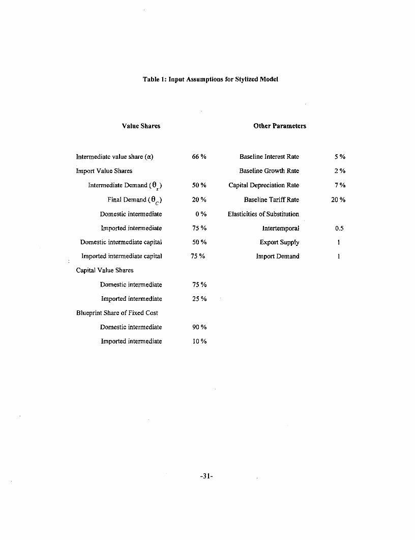
Table 1: Input Assumptions for Stylized Model

Value Shares Other Parameters

Intermediate value share (a) 66 % Baseline Interest Rate 5 %

Import Value Shares Baseline Growth Rate 2 %

Intermediate Demand (0X) 50 % Capital Depreciation Rate 7 %

Final Demand (O9 ) 20 % Baseline Tariff Rate 20 %

Domestic intermediate 0 % Elasticities of Substitution

Imported intermediate 75 % Intertemporal 0.5

Domestic intermediate capital 50 % Export Supply I

Imported intermediate capital 75 % Import Demand I

Capital Value Shares

Domestic intermediate 75 %

Imported intermediate 25 %

Blueprint Share of Fixed Cost

Domestic intermediate 90 %

Imported intermediate 10 %

Table 2: Benchmark Social Accounts (steady-state equilibrium)

L Y XD XM M I FD

PD 0.76 -0.11 -0.25 -0.40

PM -0.16 0.29 -0.02 -0.10

PX -0.66 0.33 0.33

PI 0.28 -0.28

PFX 0.24 -0.24

PL -0.34 _ 0.34

RK -0.11 -0.05 0.16

IMK I -0.11 -0.11 0.22

T I I I -0.05 0.05

Key:

Y Production of final PD Final goods

XD Domestic PM Final goods (imports)

XM Imported intermediate PX Final goods (exports)

M Imports PI Investment

I Investment PF Foreign exchange

FD Final Demand PL Wage rate

RK Return to capital

M Markup revenue

T Tariff revenue

-32-

Table 3: Estimated Welfare and Growth Effects of Tariff Reduction*

Model EV- G2010 G2050 Gterm

1. Central Assumptions 10.7 2.6 2.2 2.1

2. Spillovers 10.9 2.6 2.2 2.1

3. Constant Returns to Scale 0.5 2.0 2.0 2.0

4. Output Tax Replacement 6.7 2.5 2.1 2.0

5. Capital Income Tax Replacement 4.7 2.4 2.1 2.0

6. Capital Flows 37.0 4.2 2.7 2.2

* Parameter choices for all models are shown in table 1. Unless otherwiseindicated, all models include: lump sum replacement taxes, no spillover effect ofnew foreign varieties on the domestic cost of new blueprints, and period by periodbalance of trade constraint..

EVo Hicksian equivalent variation over the infinite horizon as a percentthe present value of benchmark steady state consumption

G2010 Average consumption growth 1997-2010G2050 Average consumption growth 1997-2050Gterm Terminal growth rate (from 2049 to 2050)

-33-

Table 4: Sensitivity Analysis

Parameter* Central Sensitivity Balance of trade constraint for each period:

Value Value EVoo G2010 G2050 Gterm

0 10.7 2.6 2.2 2.1

1. 01 0.5 0.25 4.6 2.3 2.1 2.1

2. a 0.66 0.80 11.0 2.5 2.3 2.2

3. a 0.66 0.50 11.3 2.8 2.2 2.0

4. G 0.02 0.03 14.6 3.8 3.3 3.1

5. R 0.05 0.04 13.0 2.7 2.2 2.1

6. qtDX 1 2 17.1 3.1 2.3 2.1

7. Tariff change 20% to 0% 23.7 3.4 2.5 2.2

8. Tariff change 40% to 30% 9.1 2.6 2.2 2.1

9.Tariff change 40%to0% 51.6 4.4 3.1 2.1

* The counterfactual scenarios use the sensitivity value. The central value is listed for reference only.Key:

EV°o Hicksian equivalent variation over the infinite horizonG2010 Average consumption growth 1997-2010G2050 Average consumption growth 1997-2050Gterm Terminal growth rate (from 2049 to 2050)0e Import share of intermediate inputsa Intermediate share of aggregate costG Baseline growth rateR Baseline interest rateTlDX Elasticity of transformation in aggregate production (domestic versus exports)Tariff Alternative pre-existing tariff rates and tariff reform programs (in the reference case, 20% is cut to 10%)

-34-

Table 5: Evaluation of the Uruguay Round Tariff Cuts for Five Developing Countries,with and without Product Variety Productivity Impacts

Data Welfare and Growth Estimates

import post-Country and Model intermediate share of benchmark Uruguay

value share intermediates ltariff Round tariff EV°o G20 10 G2050 Gterm

I Product Variety Productivityand Capital Flows

A. Korea 0.6 0.2 15.0 8.0 2.6 2.2 2.1 2.0

B. Malaysia 0.7 0.7 8.0 6.0 4.0 2.3 2.1 2.0

C. Thailand 0.6 0.6 32.0 25.0 7.8 2.5 2.2 2.0

D. Argentina 0.9 0.1 28.0 23.0 0.7 2.0 2.0 2.0

E. Brazil 0.6 0.1 30.0 22.0 1.4 2.1 2.0 2.0

II Constant Returns to Scaleand Capital Flows

A. Korea 0.1 2.0 2.0 2.0

B. Malaysia 0.1 2.0 2.0 2.0

C. Thailand - same as above - 0.4 2.0 2.0 2.0

D. Argentina 0.2 2.0 2.0 2.0

E. Brazil 0.1 2.0 2.0 2.0

Key : See table 3.Source : GTAP dataset for data, see Gehihar et al. (1997); and authors' estimates.

-35-

Appendix A: Growth and Welfare over the Infinite Horizon

This appendix derives algebraic relations relating changes in the growth rate of consumption to the

equivalent variation in infinite-horizon consumption. Itthen shows how these formula may be employed to

provide consistent estimates of infinite horizon welfare based on equilibrium choices over a finite horizon.

These functions relating growth to welfare are interesting for two reasons. First, they providesome intuition

as to the importance of changes in growth rates vis-a-vis the more conventional static efficiency estimates

of the welfare cost of protection. Second, these equations are required for estimating the infinite-horizon

welfare change, given welfare changes over the time horizon of the model, the terminal consumption level

and the terminal (steady-state) consumption growth rate.

We begin with a constant-elasticity of substitution utility function:

U(C) = Alc jl/p

The elasticity of intertemporal substitution is given by c=l/(l -p). The model is based on ordinal utility, so

the optimal consumer choices are unaffected by monotonic transformations of the utility function. For

example, this utility function is equivalent to:

U(C) =t=o 1-1/

The advantage of the former function is that because it is linearly homogeneous in consumption levels

(U(IC) = U(C)), a one percent change in U corresponds to a one percent equivalent variation in income.

If we let C denote a reference consumption path, and let C denote an alternative time path of consumption

levels, the equivalent variation in infinite-horizon welfare then corresponds to:

-36-

EV = ° - I

We now evaluate the equivalent variation of a permanent change in the consumption growth rate, assuming

that the initial level of consumption in period t=O is held constant. Take C, I( + g )' and

c, = ( 1 + g )'. It then follows that the equivalent variation in income is:

Er=tI - a (I +g)P I/P_I

EV = -A(--)1" II - a (i +g)P

In order to relate this expression to the calibrated equilibrium calculations such as those conducted in our

paper, it is helpful to replace the utility discount parameter, 4 by an expression based on the baseline growth

rate and interest rate. In other words, in order to compute a baseline equilibrium, we do not begin with a

given value of the utility dscountfactor. We instead assume a balanced baseline growth path with agiven

growth rate (g), and a given interest rate (r). It is then a simple matter to show that the utility discount

factor is given by:

l+r

Substituting into the equivalent variation equation, we then have:

_ _ l~~~~/pr - ( 1

EV= r-I+- ~ +g

I+9

This expression provides us with a useful check on the magnitude of welfare gains arising from our

calculations. Figure Al simply computes the Hicksian welfare metric for growth rate increases rangingfran

-37-

O to 1%. Two lines correspond to baseline growth rates of 1% and 2%. Both functions are based on a

baseline interest rate of 5% and an intertemporal elasticity of substitution equal to one half We see that

growth rate changes of a 0.5% produce welfare changes on the order of 10 to 15%, depending on the initial

growth rate. Holding constant the baseline interest rate, the welfare change increases in thebaseline growth

rate.

Figure A2 investigates the sensitivity of thisfunction to the baseline interest rate. As expected, the

higher the interest rate, the lower the welfare gain associated with a permanent change in the growth rate.

A higher interest rate implies a larger discount on future consumption increases, so that future gains in

consumption are less important.

Figure A3 illustrates the relationship between the intertemporal elasticity of substitution and the

welfare gain associated with a hafa percentage increase in the consumption growth rate. Again, the resuls

are intuitive. The higher the elasticiy of intertemporal substitution, the larger the achievable gain from an

increase in future consumption. When the intertemporal elasticity is close to zero, an increase in the growth

rate has not effect on welfare because period 0 consumption does not change. However, as the intertempord

elasticity increase from zero, the consumer benefits more as she is able to more easily substitute current

consumption for future consumption.

In our model calculations, we adopt afinite-horizon model which approximates the infinite-horizon

equilibrium. We apply terminal conditions which assure that terminal period investment is positive and

increasing with aggregate GDP (See Lau, Palke and Rutherford 1997 for details on the terminal

approximation.) Having computed equilibrium values for period 0 to T, we have an explicit utilityindex over

consumption in these periods, but this indexfails to accountfor consumption increase in the post-terminal

period We can approximate the infinite horizon welfare index, however, based on the followingfunctions

of thefinite-horizon model: (i) the welfare indexfor periods 0 to T, u ., (ii) terminalperiod consumption,

-38-

C7 and (iii) post-terminal growth, g. We produce an infinite-horizon welfareindex based on the assumption

that the economy exhibits steady-state growth at ratet from period T+l to the infinite horizon.

In order to lay out the formulae for this approximation, we begin by splitting the infinite-horizon

welfareintotwoperiods,t=0toTand t>T Weassumeagrowthrateofo_= Tc Tforthepost-termindCT

period, then:'5 )

. . I/p~~~~~~~~~~~/U(C) = E ' cfP

= [ AE d' C P + CA' { C (1 +g)()}P Ij

A L 'C p + C P / - = A' T I-A(I +g,f }When working with a calibrated model, it may be easier to begin from a reference balanced growth path.

SubstitutingforA as above, and denoting the average consumption growth rate through period t as 0,, the

equivalent variation in income can be written:

EV(f= ){ [4 -_±~I l +r) I =° t=O +r +g

+ T 1 g( r ) 1T1 I +g p- -I 1/

I+r JI I +r +g

Alternatively, this expression can be written in terms of the wefare level through period T and the level and

In the finite horizon model we use a utility function,

UT = ( S /vt CP)

in which there is no additional 'weight' on period T consumption. In the finite horizon model, a constraint on theterminal capital stock such that investment follows a steady-state growth path. Having computed the finite horizonequilibrium, we then compute the infinite horizon welfare index.

-39-

growth rate of consumption in the post-terminalperiod, i.e.

EV { 3 Up + (Ir-) I, }

In which we define: . = -b, where 0 = - and.

y (gX g) = 11+i V

In a constant growth rate model, the term y (g., g) is always unity, so the welfare then depends solely on

the utility index through model horizon and the terminal consumption level relative to the original steady-

state growth rate.

-40-

Appendix B: Benchmark Assumptions and Calibration

Consider the input data as outlined in Table 1. Scaling base yearfinal goods output to unity, we then

define imported and domestic intermediate inputs as:

x,W=o a and xD=(I -1) a'

Labor inputs for final goods production may then be inferred through exhaustion of product:

LM = ei (I-a) and L. = (1-01) (I-a).

Base year wage income is the sum of these values, L =LD +LM.

The interrnediate value share determines markups over marginal cost, and this in turn defines markip

revenues given assumed sales by firm type:

mkf = xf (1 -a), f e {D,M}

Capital returns in intermediate goods production are defined as a fraction of variable cost:

vkf = kvsf (xf - mk)

Imported inputs to intermediate goods production are also defined as a fraction of variable cost:

mxf = mvsf (xf - m9k)

Domestic inputs to intermediate production are determined by exhaustion of product:

dxf = (I-kvs,-mvs) (x,-mkp

The user cost of capital equals interest plus depreciation, so the initial capital stock in can then be inferred

from capital returns:

-41-

vkkx = f

f r+8

Fixed costs of intermediate goods production equal the sum of recurring fixed costs and blueprints. We use

a parameter fcshrf to define how these shares are separated:

fcOf = fcshr1 mkr

Blueprints do not depreciate, so the value of a firm's equity is related to the base year dividends through the

interest rate:

(1-fcshrf) mkf

ff - r

Base year furm creation is determined by the steady-state growth ram (there is no depreciation of blue-prints

in this model):

if = g f

Domestic and intermediate inputs to investment are based on the import value share in investment:

imjf = mvsIf if idf = (I-mvsi) if .

Base year capital investment in firms is sufficient to cover growth plus depreciation of the capital stock:

ixf = kxf (g + o) .

Net investment by households in the intermediate goods sector equals the total vahe of blueprint and capital

formation, less the value of markup revenue net of recurring fixed costs:

I = F_f if + ixf - (mkf + mkf - fc?

As we assume that tariff revenues are returned to the consumer in a lump sum, me must determine base year

tariff revenue and imports to final demand simultaneously. The following system of equations then

determine base year tariff revenue (7) and imports (c):

-42-

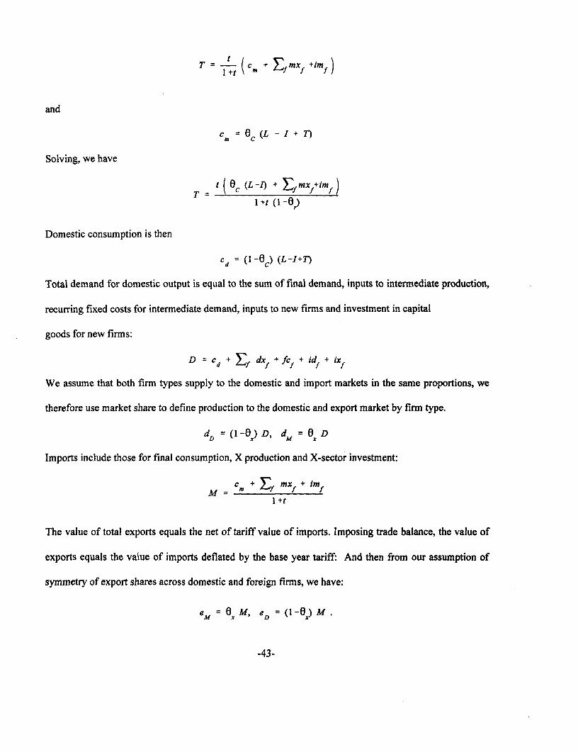
T = I +t ( C. + Efmxf im)

and

C. = 0c (L - I + 7)

Solving, we have

T=t ( (L-1) + ;,mx,+im,)

1 +t (1 -0)

Domestic consumption is then

Cd = (1-0c) (L-I+T)

Total demand for domestic output is equal to the sum of final demand, inputs to intermediate production,

recurring fixed costs for intermediate demand, inputs to new firms and investment in capital

goods for new firms:

D = cd + Er dxf + fcf + idf + ixf

We assume that both firm types supply to the domestic and import markets in the same proportions, we

therefore use market share to define production to the domestic and export market by firm type.

dD = (1-OX) D, dM =Ox D

Imports include those for final consumption, X production and X-sector investment:

M = cm + E, mx,f - im,I +t

The value of total exports equals the net of tariff value of imports. Imposing trade balance, the value of

exports equals the value of imports deflated by the base year tariff: And then from our assumption of

symmetry of export shares across domestic and foreign firms, we have:

e = M, eD = ( 1- ) M

-43-

Figure 1: Consumption Path following Tariff Reform

40

35

30 - CENTRAL, . CAPITAL FLOWS

25 CRTS@ 25/ SPILLOVERS ---

a< 20

a L00

15

n .... ............ . . . . . . . . . ... . . . . ... . .. . . . . . . .

2000 2010 2020 2030 2040 2050

.~~~~~~~~~~~~~~~~~~~~~~~~~~

Figure 2: The Real Exchange Rate following Tariff Reform

25 I -

20 -,

CENTRALCAPITAL FLOWS

15 CRTS. . . . . .= =. . . ......... SPILLOVERS -

10 7

0

I01

-10 1i0 0 20 , 2000 2010 2020 2030 2040 2050

Figure 3: Interest Rate following Tariff Reform8.5 , . .

CENTRAL7.5 l CAPITAL FLOWS

CRTS2 7 i, SPILLOVERS

6.5 A

64

5.5 IIt

5 ; ;: -- ------ ,----------------------- -- ,--

2000 2010 2020 2030 2040

Figure 4: Domestic Firms following Tariff Reform

250-------

200

CENTRALCAPITAL FLOWS

150 CRTS

SPELLOVERS

a)100

0 50

-502000 2010 2020 2030 2040 2050

Figure 5: Foreign Firms following Tariff Reform

100 ,/\ . .I 00~~~~

80 /| ''\\ ~~~~~~~~CENTAGrL

60 ~~~~~~~~~~~CAPITAL FLOWS60 , , |CRTS

., SPILLOVERS --

40 l

20

X g ~~.. ... . . .. ... .... ,,,..... .. . ....... ..... .... .. ,...:.,j. .... . .. ... .. . .

-20X

-20,

-40 , , , 2000 2010 2020 2030 2040 2050

Figure 6: Consumption Paths forAlternative Replacement Taxes

40 1 - - ,

35

CENTRAL30 CAPITAL FLOWS25" !OUTPUT TAX

CAPITAL TAX

20

0 20

X1510

1510 __ _

2000 2010 2020 2030 2040 2050

Policy Research Working Paper Series

ContactTitle Author Date for paper

WPS1952 Enterprise Isola;ion Programs in Simeon Djankov August 1998 R. VoTransition Econor.iss 33722

WPS1953 Trade Policies and Incentives M G5arry Purseil August 1998 L. TabadaIndian Agriculture: Methodology, 36896Backgrounid Statistics and Proteclion,and incentive indicators, 1965-95--Backgrounld Paoer 1, Suger andSugarcane

WPS1954 Politicians and Firms in SEven Stuni C!e4ee .s A.i-u5t 1998 R. VoCentral and Eastern European Simneon D;arlKo-v 33722Countries

WPS1955 Appraising Workfare Prcgrams Martin Ravaliicr A u g -st i998 P. Sader33902

WPS1956 Benefit Incidence and the Timing Peter Lanjouwv A..icic. 198 P. Saderof Program Capture Martin Ravaition 3.3902

WPS1957 Bidding for Concessions Michael Kl,e n nCc 5 ;3 a Oytarg37 161

WPS1958 Total Strar,gers or SCul Niates? J. Luis Guash .4u ; 8. TroncosoAntidumping and Competition Sarath Rajapatirane 37826Policies in Latin America and theCaribbean

WPS1959 Is There a Credit Crunch in Wei Ding A g -998 F FernandesEast Asia? lIker Doriar, 80453

Giovarvni Fecr.

WPS1960 Calm After the Storms: Income Francisco H. r. Fe-reirna A g -. 139 G. iIogonDistribution in Chile 1987-94 Julie A. Litchfield 33732

WPS1961 Protecting the Environment and the Gunnar S. Eskeland Augu st '998 C. BernardoPoor: A Public Goods Framework Chingying K.ong 31 143Applied to Indonesia

WPS1962 The Political Economy of Geore R. G Ciaron A s '998 P. Sintim-AboagyePrivatization An Empirical AnaiysIs Robert -Cii 38526of Bank. F'rivatization in Argenmna

WPS1 963 Commodity Risk Manaecement anld D F. an Arn z 1998 P. KokilaDevelopment .a, s V-ara, s 33715

Ni?nane vab.;i,ri

WPS1964 Pubiic Investment and Economic Uk-ituh Lachi 98 C. LazcanoGrowth in Mexico David Aian Asccnoauoe 37776

Policy Research Working Paper Series

ContactTitle Author Date for paper

WPS1965 Manufacturing Firms in Developing James Tybout August 1998 L. TabadaCountries: How Well Do They Do, 36869and Why

WPS1966 Sulfur Dioxide Control by Electric Curtis Carlson August 1998 T. TourouguiUtilities: What Are the Gains from Dallas Burtraw 87431Trade? Maureen Cropper

Karen L. Palmer

WPS1967 Agriculture and the Macroeconomy Maurice Schiff August 1998 A. ValdesAlberto Valdes 35491

WPS1968 The Economics and Law of Rent Kaushik Basu August 1998 M. MasonControl Patrick Emerson 30809

WPS1 969 Protecting the Poor in Vietnam's Dominique van de Walle September 1998 C. BernardoEmerging Market Economy 31148