WP-2015-018

Trade Liberalisation and Women's Employment Intensity: Analysisof India's Manufacturing Industries

Purna Banerjee and C. Veeramani

Indira Gandhi Institute of Development Research, MumbaiJune 2015

http://www.igidr.ac.in/pdf/publication/WP-2015-018.pdf

Trade Liberalisation and Women's Employment Intensity: Analysisof India's Manufacturing Industries

Purna Banerjee and C. VeeramaniIndira Gandhi Institute of Development Research (IGIDR)

General Arun Kumar Vaidya Marg Goregaon (E), Mumbai- 400065, INDIA

Email(corresponding author): veeramani@igidr.ac.in

AbstractIn the context of increasing contribution of developing countries in world trade, an important question

is whether trade can be used as an instrument to stimulate higher participation of women in the labour

market? Trade and industrial liberalization undertaken during the 1990s and 2000s marked the end of

India's nearly four decade experiment with state directed, heavy industry based, and import substituting

industrialization. In this context, we analyse the role of various trade and technology related factors in

determining female employment intensity (FEI), in a panel of India's manufacturing industries for the

period 1998-2008. We find that import tariff rates exert a negative effect on FEI, supporting the

hypothesis that firms, when exposed to international competition, tend to reduce costs by substituting

male with female workers. Further, the relative demand for female workers increases to the extent that

trade liberalization leads to resource reallocation in favour of unskilled labour intensive industries

where India holds comparative advantage. By contrast, greater use of new technology and capital

intensive production biases the gender composition of workforce against females. Liberalization has not

led to large growth of female employment in India's organized manufacturing sector because the

resource reallocation effect has not been strong enough to offset the negative technology effect.

Keywords: female employment intensity, trade liberalization, manufacturing, India

JEL Code: J16, J21, J82, F16, F66

Acknowledgements:

Earlier versions of the paper were presented at the 55th Indian Society of Labour Economics (ISLE) Conference 2013 (JNU, New

Delhi), IMR Doctoral Conference, (IIM, Bangalore) and IGIDR Silver Jubilee Conference (IGIDR, Mumbai). The authors are

thankful to participants for their helpful comments.

1

Trade Liberalisation and Women’s Employment Intensity: Analysis of India’s Manufacturing

Industries

Purna Banerjee and C. Veeramani

Indira Gandhi Institute of Development Research (IGIDR)

Gen A K Vaidya Marg, Goregaon East, Mumbai - 400065, India

Email: : purna@igidr.ac.in , veeramani@igidr.ac.in

1. Introduction

Promotion of gender equality and empowerment of women is one of the Millennium Development

Goals (MDGs) that the international community, under the aegis of the United Nations, has been

pursuing since 2000 (UN, 2014). Needless to say, creation of greater employment opportunities for

women is crucial for the achievement of this goal. Furthermore, participation of women in productive

employment plays an instrumental role in the achievement of several other MDGs such as ending

hunger and poverty, reducing child mortality, improving maternal health and attaining universal

primary education. A number of studies show that having an independent source of income gives

women greater bargaining power within the household, which in turn leads to better health outcomes

for children (see Duflo, 2012 for a survey).

In the context of increasing contribution of developing countries to world trade, an important question

is whether trade can be used as an instrument to stimulate higher participation of women in the labour

market? Greater international integration of the domestic market is expected to improve a country’s

export competitiveness and growth through efficient resource allocation, greater specialization,

diffusion of international knowledge and heightened competition. These changes, in turn, are likely to

exert major impacts on employment and other labour market outcomes, which could be gender

differentiated. There are four different channels through which trade liberalization can exert a gender

differentiated impact on employment: cost reduction effect, resource reallocation effect, technology

effect and scale effect. These channels are discussed in detail in Section 2.

2

India has initiated a process of major structural adjustment since the early 1990s. Trade and industrial

liberalization undertaken during the 1990s and 2000s marked the end of India’s nearly four decade

experiment with state directed, heavy industry based, and import substituting industrialization. The

quantitative restrictions (QRs) on importing capital goods and intermediates were mostly dismantled

in 1992. However, the ban on importing consumer goods continued, with some exceptions, until the

late 1990s. Apart from the removal of QRs, import tariff rates in the manufacturing industries were

also gradually reduced. Following the tariff reductions introduced in the March 2007 budget, India

has emerged as one of the world’s low protection and open industrial economies (Pursell et al, 2007).

A number of empirical studies, reviewed in the next section, show that trade liberalization and export

orientation have had a beneficial effect on women’s employment opportunities in several developing

countries. However, India has witnessed a declining trend in female workforce participation rates

since the late 1990s1. Further, India’s labour force participation rate (LFPR) for women, particularly

in the urban sector, is much lower than the norm for countries with similar levels of development

(Bhalla and Kaur, 2011; Thomas, 2012). Thus, unlike in the case of other developing countries,

liberalization has not led to higher employment opportunities for women in India. However, the

trends observed at the aggregate level could mask important heterogeneities across industry groups.

In order to understand why trade liberalization in India has failed to generate a beneficial impact on

female employment, it is necessary to consider variation across industries both in terms of female

employment intensity and degree of trade openness.

In this paper, we analyse the role of various trade and technology related factors in determining

female employment intensity (FEI), in a panel of India’s organized (formal) manufacturing industries

for the period 1998-2008. To the best of our knowledge, these issues have not been empirically

1 This trend is particularly stark in rural areas. See Mazumdar and Neetha (2011), Chowdhury (2011), Kannan and

Raveendran (2012), Chen and Raveendran (2012) and Abraham (2013). Rangarajan et al (2011, 2014) who argue that the

declining labour force participation rate (LFPR) of women is mainly on account of withdrawals of women from the

workforce due to rising participation in education among young females as well as the general improvement in rural income.

While most of these studies posit some possible explanations for the broad trends in female LFPR, there are very few studies

that econometrically test the underlying hypotheses using detailed data at the industry level.

3

examined in the context of India, a country which is home to about 17 percent of the world’s female

population and to roughly one-third of the world’s poor.

The focus of the current work on organized manufacturing industries is motivated by the fact that

these jobs are usually more sought after compared to poorly paid informal work. Organized sector

jobs provide a number of benefits in terms of higher wages, higher job security, better working

conditions and greater opportunities for upward mobility2. By contrast, a job in the unorganized

sector, more often than not, is a fall back option when formal sector jobs are not available.

Understanding the determinants of FEI in the organized manufacturing industries is crucial as higher

employment of women in these industries usually reflect broad improvements in the quality of their

employment. While data availability dictated the time period of our analysis (1998-2008)3, it may also

be noted that the most far-reaching trade liberalization initiatives, especially in consumer goods

industries, were undertaken in India during the study period, since the late 1990s.

The key results from this paper may be summarized as follows. The overall FEI, defined as the share

of female employment in total employment, in the formal manufacturing sector in India is quite low at

about 11%. However, FEI varies considerably across industries with the values being the highest and

growing in industries which are unskilled labour intensive and export oriented. We find that import

tariff rates exert a negative effect on FEI supporting the hypothesis that firms, when exposed to

international competition, tend to reduce costs by substituting male with female workers. The relative

demand for female workers would also increase to the extent that trade liberalization leads to resource

reallocation in favour of unskilled labour intensive industries where India holds comparative

advantage. The resource reallocation effect, however, has not been strong enough to generate huge

employment opportunities for women in India. Inflow of foreign technology, via FDI and capital

goods imports, has created a bias against female employment.

2 For the year 2009-10, organized manufacturing sector accounted for 10.52% of employment and 65.02% of value added in

the total manufacturing sector (Kapoor, 2014). 3 We use data at the 4-digit ISIC level from the UNIDO’s industrial database. For India, gender-wise data on manufacturing

employment is available at the 4-digit level since 1998 only.

4

The rest of the paper is organized as follows. Section 2 provides a review of related theoretical and

empirical literature. Section 3 provides a descriptive account of the general trends and patterns of

female employment in India’s organized manufacturing sector. Section 4 sets out the hypotheses

concerning the effects of various trade and technology related variables on FEI. This section also

provides the definition of the various explanatory variables. Section 5 discusses the regression

methodology and data sources. Results of the econometric analysis are discussed in Section 6.

Conclusions and implications of the findings are presented in Section 7. A detailed description of data

and variables is given in the Appendix (see Table A1).

2. Women’s Employment and Trade Liberalization: Theoretical Framework and Empirical

Literature

2.1 Theoretical Framework

The various channels through which trade liberalization can result in gender differentiated

employment outcome needs clear articulation. Analytically, it is useful to distinguish four separate

mechanisms by which a change in trade policy can exert an impact on FEI.

First, trade liberalization has a cost reduction effect resulting from heighted competitive pressure from

imports. Faced with international competition, firms may adopt a strategy of feminization of labour

force as women provide ‘cheap and flexible’ labour compared to men [Cagatay and Ozler, 1995;

Elson, 1999; Standing, 1999]. It has been observed that women workers are intensively employed in

industries where profit margins are protected by reducing labour costs, extending hours and

decreasing the numbers of formal production workers (Standing, 1999)4.

4 Furthermore, an implication of the Becker model of discrimination (1957) is that increased product market competition will

drive out costly discrimination against women in the labour market (Black and Brainerd, 2004). Thus, if trade liberalization

increases product market competition, employers may find it unaffordable to indulge their “taste for discrimination” leading

to an increase in the relative employment of women.

5

Second, there is a resource reallocation effect resulting from trade-induced changes in the pattern of

specialization. According to the Heckscher-Ohlin (H-O) model, countries specialize in and export

goods that use intensively the factors of production with which they are relatively abundantly

endowed. Given that developing countries, like India, are abundantly endowed with unskilled labour,

their true comparative advantage lies in industries that intensively use unskilled labour rather than

physical capital or skilled labour5. Therefore, it may be expected that trade liberalization would

stimulate faster growth of unskilled labour-intensive industries in India. This, in turn, can lead to an

increase in the relative employment of female workers if, as is often the case, unskilled-labour

intensive industries employ more female than male workers. In developing countries, such as India,

female employment intensity is generally higher in unskilled -labour intensive industries due to the

fact that the average female worker has lower educational attainment, and hence less skilled, than the

average male worker6.

Third, there is a technology effect associated with trade liberalization. While cost reduction and

resource reallocation effects may imply an increase in FEI, rapid inflow of foreign technology, via

FDI and increased imports of capital goods, may create a bias in favour of male employment. This

bias could arise because the new technology, mainly designed in the skill abundant industrialized

world, is skill-biased and exhibits capital-skill complementarities in production (Krusell et al, 2000)7.

Thus, the relative demand for male workers may rise if, as is often the case, the skill level of the

average male worker is higher than that of the average female worker8.

5 Educational attainment data for the 2010 shows than more than half of India’s population have either no schooling or only

primary attainment (Barro and Lee, 2013). 6 As per the NSSO data, the average woman had 2.1 years lesser education than the average man in 2007-08 (Bhalla and

Kaur, 2011). Fontana (2009) reviewed a large number of studies covering many countries and concludes that trade

liberalization benefits women the most in countries that are abundant in unskilled labour and have a comparative advantage

in the production of basic manufactures (Fontana, 2009). This is because women are disproportionately represented among

unskilled workers. 7 Capital-skill complementarity implies that the elasticity of substitution between capital equipment and unskilled labour is

higher than that between capital equipment and skilled labour (Krusell et al, 2000). 8 Even if male and female workers possess the same level of skill, employers may still prefer male workers for technology

intensive tasks. The theory of statistical discrimination provides an explanation for this preference. This theory states that

when employers have limited information about individual job seekers, they tend to use easily observable characteristics

such as gender or race to infer the expected productivity of individuals (Arrow, 1973; Aigner and Cain, 1977). In the case of

technology-intensive (high-skilled) jobs, firms may attempt to minimize training and replacement costs by choosing workers

with low quit propensity. Thus, if the perceived quit propensity is higher for women workers, employers may adopt a skill

6

Finally, there is also a scale effect which arises, ceteris paribus, when trade liberalization causes an

overall expansion of output and employment. The scale effect could be gender neutral if employment

for males and females grow at the same rate. Since we have no strong priors regarding the direction of

the relationship between scale and FEI, we leave this to be determined empirically.

Thus, on theoretical grounds, trade liberalization can exert a positive or negative impact on aggregate

female employment depending on the relative strength of the different channels. While the cost

reduction and resource reallocation effects can raise the employment share of women workers, the

technology effect can act as a countervailing force. There is a need to empirically analyse the different

channels through which liberalization affects female employment and this provides the motivation for

analysing the role of trade and technology related variables in influencing FEI.

2.2. Review of Related Empirical Studies

Aside from the theoretical reasons outlined in the previous section, there exists strong empirical

evidence suggesting that trade liberalization exerts differential impact for male and female

employment9. Based on a cross country analysis, Cagatay and Ozler (1995) concluded that countries

that have undertaken structural adjustment programs have recorded an increase in the female share of

their labour force. In the context of developing countries, in particular, the forces of global

integration have generally had a beneficial effect on women’s employment (Wood, 1991; Joekes,

1995; Mehra and Gammage, 1999; Nordas, 2003; Fontana 2009). The employment gains for women

have been driven by export-oriented industries, such as clothing, footwear and electronics assembly,

retention strategy by hiring male workers for tasks that involve high training and replacement costs. Given the social

customs related to marriage, child bearing and child rearing in developing countries such as India, employers may believe

that women are more likely to quit a job than man is. Therefore, women are likely to get relegated to the technologically

simpler tasks (with lower training and replacement costs) while men perform technologically complex tasks. 9 Keeping with the focus of the present paper, our review is confined to empirical studies analyzing the impact of trade

liberalization on female employment in the manufacturing sector. Studies focusing other sectors (agriculture, services and

informal sector) are not taken into account. In any case, employment gains for woman worker through export-orientation

appear to be more common in the manufacturing sector than in other sectors (Fontana, 2009). Also, studies analyzing the

impact of trade on gender wage inequality are not considered here. Interested readers are referred to Duflo (2012), who

provides a comprehensive survey.

7

mostly based in export processing zones. Women comprise between 53% and 90% of the employed in

many export sectors in middle-income developing countries (Korinek, 2005). These findings are

consistent with the prediction of the H-O model that opening up trade would lead to an expansion of

unskilled labour intensive industries in developing countries. Women workers benefit from this

process as their employment is largely concentrated in unskilled labour-intensive industries10

.

In addition to the cross country studies referred above, a number of country case studies also found

that trade liberalization had a positive effect on women’s employment opportunities via export

expansion. The gains in female employment are particularly pronounced in the four East Asian Tigers

(Hong Kong, Singapore, South Korea and Taiwan). Between 1966 and 1996, female labour force

participation rate increased from 24.2 percent to 51.5 percent in Singapore, from 32.6 percent to 45.8

percent in Taiwan and from 31.5 percent to 48.7 percent in South Korea. For Hong Kong, this

proportion increased from 36.8 percent in 1961 to 49.2 percent in 1996 (Chu, 2002). In line with the

experience of East Asia, South East Asian countries (Malaysia, Indonesia, Philippines and Thailand)

have witnessed a substantial increase in female employment in labour-intensive export-oriented

industries (Pearson 1998, Fontana 2009). While South Asia as a group records lower FEI compared

to East and South East Asia, export oriented garment industries of Bangladesh and Sri Lanka have

recorded significant increase in female employment (Mehra and Gammage, 1999; Nordas, 2003;

Rahman and Islam, 2013).

The major non-Asian developing countries where export expansion led to higher FEI include

Mauritius (Sub-Saharan Africa), Mexico (Latin America) and Turkey. There exists a consensus that

mobilization of female labour in the export processing zones played a key role in the export success of

Mauritius since the mid-1970s (Milner and Wright, 1998; Subramanian and Roy, 2001; Nordas,

2003). Aguayo-Tellez et al (2010) find that women’s relative employment position improved

10 The cross-country analysis by Wood (1991) found that expansion of manufactured exports to developed countries (North)

has been strongly associated with increases in the female intensity of manufacturing employment in the developing countries

(South). On the other hand, trade expansion with developing countries was found to exert a negative effect on FEI in most

developed countries (Kucera and Milberg, 2007).

8

significantly in Mexico during the 1990s, a period that witnessed major trade liberalization under

NAFTA. Their empirical analysis showed that trade liberalization resulted in substantial labour

reallocation across industries, shifting employment towards initially female-intensive sectors. They

also find that Mexico’s tariff reduction as well as its access to the US market via exports led to greater

employment opportunities for women11

. Cagatay and Berik (1991) and Ozler (2000) found that

greater export orientation was positively associated with female employment share in Turkish

manufacturing. Baslevent and Onaran (2004), however, find that a general positive effect of export

orientation is only observed in the case of non-married women in Turkey. In the case of married

women, the positive effect is limited to only conventionally female-dominated industries and with a

time lag.

While trade liberalization is likely to raise women’s employment in the early phase of export-driven

growth in developing countries, the process can be reversed in the later phases as export production is

restructured and becomes technologically more sophisticated. As noted in the case of the East Asian

and South-East Asian economies, there has been a process of de-feminization of the workforce as the

country proceeds on the development path (Berik, 2005). In South Korea, for example, female

employment expanded significantly during the 1970s and early 1980s when export production was

concentrated in labour intensive and low technology industries such as garments, footwear and simple

consumer goods (Kim and Kim, 1995; cited in Mehra and Gammage (1999)). However, the number

of female workers declined considerably during the late 1980s and early 1990s as South Korea’s

export composition changed in favour of technologically sophisticated products such as semi-

conductor devices and computer products. Similar trends were also observed in the export processing

zones of countries such as Mexico, Mauritius, Malaysia and Singapore (Fontana, 2009).

As noted earlier, unlike in the case of other developing countries, liberalization has not led to higher

employment opportunities for women in India. Why has liberalization failed to generate a beneficial

impact on female employment? The impact of trade liberalization on aggregate female employment is

11 See Nordas (2003) for reference to the earlier studies on Mexico.

9

determined by the relative strengths of different channels. For example, we may not observe an

increase in aggregate FEI if the technology effect dominates over other effects. While trade

liberalization might have led to an increase in FEI in some industry groups, technology related factors

may be forcing females out of employment in other industries. The trends observed at the aggregate

level could mask important heterogeneities across industry groups. Thus, in order to properly

understand the impact of liberalization on FEI, it is necessary to consider heterogeneities across

industries as well as the relative importance of different channels. To the best of our knowledge,

these issues have not been empirically examined in the context of Indian industries12

.

3. Female Employment in Manufacturing: General Trends and Patterns

3.1 Aggregate Trends

Figure 1 depicts the trends in the number of male and female workers engaged in India’s organized

manufacturing sector during the period 1998-2008. As expected, the number of female workers lags

far behind male workers, for e.g., 1.2 million female workers were employed in 2008 compared to 9.7

million male workers. During the beginning of the period, the number of female workers declined

from about 1.1 million in 1998 to 0.8 million in 1999. Detailed examination of data shows that this

decline was entirely driven by just one industry group – tobacco products (ISIC 1600) – where the

number of female employees declined dramatically from more than 0.3 million in 1998 to less than

0.09 million in 199913

. Subsequently, since 1999, female as well as male employment registered an

increase at 4% per annum. Since male employment grew at the same rate as female employment,

female employment intensity (FEI) remained roughly constant during 1999-2008 (see Figure 1). It is

evident that FEI in Indian manufacturing, with an average value of 11.3% for 1999-2008, is quite low

by international standards. Thus, at the aggregate level, we do not observe a process of feminization in

12 A few of the existing econometric studies focus on the importance of supply side factors related to demography, control

over assets, socio-cultural factors, household characteristics etc. in explaining the labour force participation rate (LFPR) for

women (Bhalla and Kaur, 2011; Srivastava and Srivastava, 2010). 13 The ‘bidi’ manufacturing industry accounts for over 90% of female employment in the group ‘tobacco products’. The

employment decline in tobacco is mainly driven by ‘bidi’ manufacturing, an industry which traditionally employs large

number of female workers. This industry also experienced a significant decline in the value of output in this period.

10

India’s organized manufacturing sector. However, as noted earlier, the trends observed at the

aggregate level could mask important heterogeneities across industry groups, to which we turn now.

Insert Figure 1 here

3.2 Gender-wise Distribution of Workers across Industry Groups

Having shown the aggregate trends, we now turn to discuss the gender-wise distribution of workers

across industry groups (at the 2-digit ISIC level) within manufacturing for selected years - 1999, 2003

and 200814

. In order to view labour market changes through the lens of Heckscher-Ohlin model, it is

useful to club industries based on their trade orientation and factor intensity. To this end, industries at

the 4-digit ISIC level are classified into three broad groups based on trade orientation: exporting,

import competing and non-competing15

. Further, we classify industries into three factor intensity

based groups: primary & resource intensive, unskilled labour intensive and capital intensive16

.

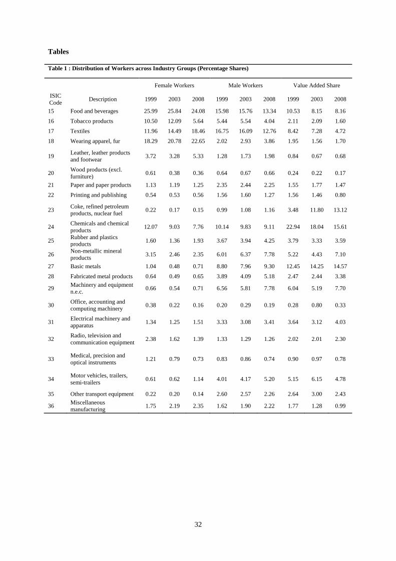
Table 1 reports the percentage share of female (male) workers in different industry groups in total

female (male) manufacturing employment17

. The table also contains information regarding the share

14 As noted above, female employment declined sharply in 1999 over the previous year, which can be clearly seen as an

aberration from the general trend (see Figure 1). We choose 1999, instead of 1998, in order to avoid any bias from this

change caused by just one industry group (tobacco products). 15 In order to classify industries according to trade orientation, we follow the methodology proposed by Krueger (1981) (see

also Krueger et al 1981; Erlat, 2000). Let C stands for consumption, where Q is production, X is exports and

M is imports. Then, T is defined as: = . If the value of T is less than zero, we say that

the industry in question is ‘exporting’. Based on the extent to which imports dominate over exports, industries with values of

T greater than zero are classified into two categories: import competing and non-competing. We consider 0.30 as the cut-off

and classify all industries with values of T above this cut-off as non-competing, while industries with T lying between 0 and

0.30 are classified as import competing. 16 We closely follow the factor intensity classification of International Trade Centre (ITC), adapted by Hinloopen and van

Marrewijk (2008). The classification is available at: (http://www2.econ.uu.nl/users/marrewijk/eta/intensity.htm) (Viewed on

14 June 2014). A total number of 240 items, at the 3-digit SITC level, have been grouped into five categories: primary,

natural-resource intensive, unskilled-labour intensive, human capital-intensive, technology-intensive, and unclassified. For

our purpose, we have matched the 3-digit SITC codes with the 4-digit ISIC codes. Our definition of capital-intensive sector

includes the industries belonging to technology as well as human capital- intensive groups. We have also clubbed the

primary and natural resource-intensive groups.

17 Percentage share of female employment in a given industry group i is defined as: 100

i

iii fwfwfs , where

the numerator, fwi, is the number of female workers employed in industry group i while the denominator is the total female

employment in manufacturing. The percentage share of male employment has been calculated in the similar manner.

11

of different industry groups in manufacturing value added. It is clear that female employment is

highly concentrated in a handful of industries while male employment shows greater dispersion. Just

six industry groups accounted for about 84% of female employment in 2008, which includes Food

and beverages (24%), Wearing apparel (23%), Textiles (18%), Chemicals (8%), Tobacco products

(6%), and Leather products (5%). These industries, however, accounted for only 45% of total male

employment. Male employment tends to be concentrated in sectors such as Machinery, Transport

equipment, Rubber and plastics, Metal products etc.

Insert Table 1 here

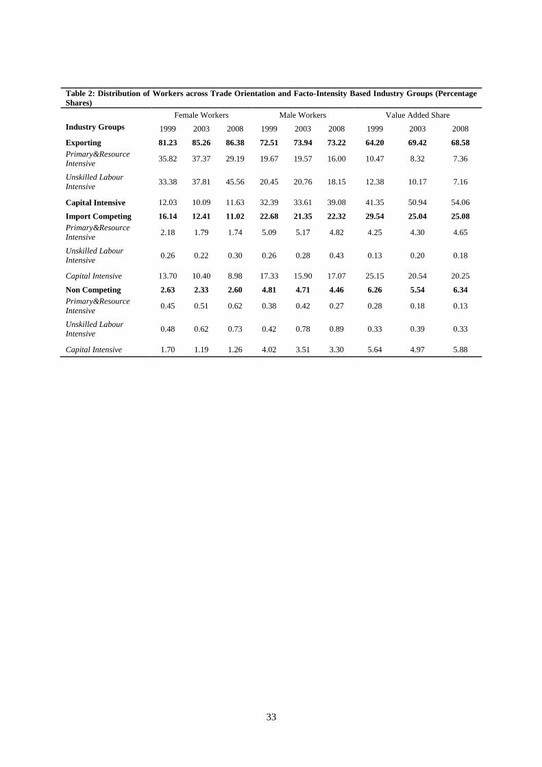
In Table 2, we present the distribution of female manufacturing workers across the industry groups

classified on the basis of trade orientation and factor intensity. It is evident that the exporting sector is

the largest contributor of employment for both female and male workers. However, female workers

are more heavily concentrated in this sector compared to their male counterparts and increasingly so.

For example, in 2008, a whopping 86% of the total female workers were engaged in the exporting

sector while the corresponding figure for the male workers was 73%. Within the exporting sector,

female workers are mainly employed in unskilled labour-intensive industries, increasing its share in

total female employment from 33% in 1999 to 46% in 2008 (Table 3)18

. The import competing sector

stands next to exporting sector both for females and males.

Finally, comparing the changes in the distribution of employment with that of real value added in

Table 2, we can observe an important contrast in the growth pattern of male and female employment.

While female workers are increasingly getting concentrated in slow growing unskilled-labour

intensive exporting industries, male employment growth is seen primarily in fast growing capital

intensive exporting industries.

18 Within the exporting sector, the pattern of male employment looks completely different from that of female employment.

Male workers in the exporting sectors are increasingly concentrated in capital-intensive industries, with a share of 32% in

1999 and 39% in 2008 (Table 2). In contrast, capital-intensive exporting industries accounted for just 12% of total female

workers both in 1999 and 2008.

12

Insert Table 2 here

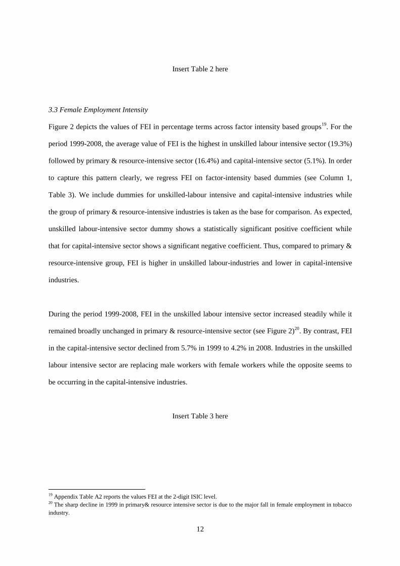
3.3 Female Employment Intensity

Figure 2 depicts the values of FEI in percentage terms across factor intensity based groups19

. For the

period 1999-2008, the average value of FEI is the highest in unskilled labour intensive sector (19.3%)

followed by primary & resource-intensive sector (16.4%) and capital-intensive sector (5.1%). In order

to capture this pattern clearly, we regress FEI on factor-intensity based dummies (see Column 1,

Table 3). We include dummies for unskilled-labour intensive and capital-intensive industries while

the group of primary & resource-intensive industries is taken as the base for comparison. As expected,

unskilled labour-intensive sector dummy shows a statistically significant positive coefficient while

that for capital-intensive sector shows a significant negative coefficient. Thus, compared to primary &

resource-intensive group, FEI is higher in unskilled labour-industries and lower in capital-intensive

industries.

During the period 1999-2008, FEI in the unskilled labour intensive sector increased steadily while it

remained broadly unchanged in primary & resource-intensive sector (see Figure 2)20

. By contrast, FEI

in the capital-intensive sector declined from 5.7% in 1999 to 4.2% in 2008. Industries in the unskilled

labour intensive sector are replacing male workers with female workers while the opposite seems to

be occurring in the capital-intensive industries.

Insert Table 3 here

19 Appendix Table A2 reports the values FEI at the 2-digit ISIC level. 20 The sharp decline in 1999 in primary& resource intensive sector is due to the major fall in female employment in tobacco

industry.

13

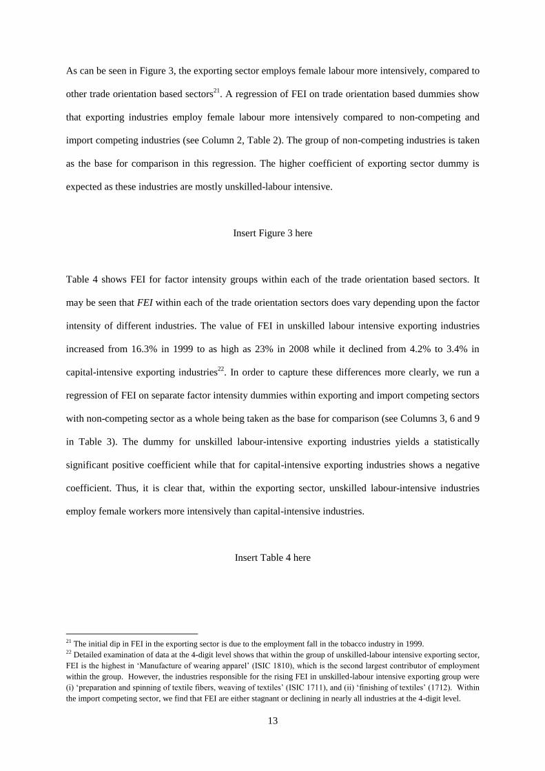
As can be seen in Figure 3, the exporting sector employs female labour more intensively, compared to

other trade orientation based sectors21

. A regression of FEI on trade orientation based dummies show

that exporting industries employ female labour more intensively compared to non-competing and

import competing industries (see Column 2, Table 2). The group of non-competing industries is taken

as the base for comparison in this regression. The higher coefficient of exporting sector dummy is

expected as these industries are mostly unskilled-labour intensive.

Insert Figure 3 here

Table 4 shows FEI for factor intensity groups within each of the trade orientation based sectors. It

may be seen that FEI within each of the trade orientation sectors does vary depending upon the factor

intensity of different industries. The value of FEI in unskilled labour intensive exporting industries

increased from 16.3% in 1999 to as high as 23% in 2008 while it declined from 4.2% to 3.4% in

capital-intensive exporting industries22

. In order to capture these differences more clearly, we run a

regression of FEI on separate factor intensity dummies within exporting and import competing sectors

with non-competing sector as a whole being taken as the base for comparison (see Columns 3, 6 and 9

in Table 3). The dummy for unskilled labour-intensive exporting industries yields a statistically

significant positive coefficient while that for capital-intensive exporting industries shows a negative

coefficient. Thus, it is clear that, within the exporting sector, unskilled labour-intensive industries

employ female workers more intensively than capital-intensive industries.

Insert Table 4 here

21 The initial dip in FEI in the exporting sector is due to the employment fall in the tobacco industry in 1999. 22 Detailed examination of data at the 4-digit level shows that within the group of unskilled-labour intensive exporting sector,

FEI is the highest in ‘Manufacture of wearing apparel’ (ISIC 1810), which is the second largest contributor of employment

within the group. However, the industries responsible for the rising FEI in unskilled-labour intensive exporting group were

(i) ‘preparation and spinning of textile fibers, weaving of textiles’ (ISIC 1711), and (ii) ‘finishing of textiles’ (1712). Within

the import competing sector, we find that FEI are either stagnant or declining in nearly all industries at the 4-digit level.

14

Further, it may be noted that capital-intensive exporting industries employ relatively fewer female

workers compared to non-competing sector as a whole. Irrespective of trade orientation, primary &

resource-intensive industries employ fewer female workers compared to unskilled labour intensive

industries. Compared to capital-intensive industries, however, primary & resource-intensive industries

show higher FEI in both exporting and import-competing sectors.

Overall, it is clear that women are intensively employed in unskilled labour intensive exporting

industries where India has a comparative advantage. By contrast, import competing and non-

competing industries record lower FEI. Irrespective of trade orientation, capital-intensive industries

tend to employ relatively more male workers. This is consistent with the argument that technological

modernization generally creates a bias in favour of male workers. While certain industry subgroups

indeed witnessed a process of feminization, trade liberalization did not lead to a major overall

employment gain for female workers as the traditionally female worker intensive industries recorded

lower growth rate of output compared to male worker intensive industries. Thus, contrary to the

expectation, the reallocation effect does not seem to have been favourable for women workers in

India. In the concluding section, we provide an explanation for this unexpected outcome.

It is clear that there exist considerable variation in the gender composition of workforce across

industries and that industry-specific factors related to trade orientation and technology plays an

important role in determining this variation. The rest of the paper deals with an econometric analysis

of the industry-specific determinants of FEI in a panel of Indian manufacturing industries.

4. Hypothesis and Variables

In what follows, we set out various hypotheses concerning the impact of different trade and

technology related characteristics on FEI across industries. Formulation of the hypotheses and choice

of the corresponding variables have been motivated in the light of our earlier discussion of the various

channels through which trade liberalization can exert an impact on FEI.

15

(a) Cost Reduction Effect

Since the onset of the trade liberalization process, firms in India’s domestic industries, which had

been operating under protective umbrellas, have been forced to respond to competitive pressure from

imports. Removal of product market distortions, through reduction of tariff and non-tariff barriers, has

compelled domestic producers to rationalize their production structure and reduce costs. In several

economies, this led to higher female employment since women provide ‘cheap and flexible’ labour

(Standing, 1999). In order to capture the cost-reduction effect of trade liberalization on female

employment we use the variable TARit defined as the average import tariff rate in industry i and year t.

(b) Resource reallocation effect

As discussed earlier, given the abundance of unskilled labour in the country, India’s comparative

advantage lies in industries which intensively employ this factor. Thus, trade liberalization would lead

to specialization and expansion of unskilled labour-intensive industries. The process of resource

reallocation, along the lines of comparative advantage, in turn, implies higher employment

opportunities for women assuming that the demand for women workers is concentrated at the lower

end of the skill spectrum. In order to capture this effect, we employ a variable EOit defined as the ratio

of exports to output in industry i at time t (

. The values of EOit, which

measures the export orientation of an industry, are generally higher in industries where a country has

comparative advantage – that is, unskilled labour-intensive industries in the case of developing

countries like India. Thus, we expect that EOit would influence FEI positively.

The counterpart of above argument is that India has a comparative disadvantage in capital and skill

intensive industries. Thus, trade liberalization may lead to a contraction of capital and skill intensive

industries and India is expected to become a net importer of these products. We use import

penetration rate (IMit), defined as the ratio of imports to apparent consumption in industry i, as an

explanatory variable (

where the denominator is measured as the

16

difference between output and net exports). Values of IMit are expected to be higher in industries

where India has a comparative disadvantage – that is capital and skill-intensive industries. These

industries are likely to exhibit capital-skill complementarities in production and hence lower FEI. We

expect this variable to exert a negative effect on FEI.

A high level of fragmentation (vertical specialization) based trade, which occurs when countries

specialize in particular stages of a good’s production sequence rather than in the entire good, has been

an important feature of globalization (Feenstra, 1998; Hummels et al, 2001; Athukorala, 2011). This

type of trade is the result of the increasing interconnected production processes that form a vertical

trading chain stretching across many countries, with each country specializing according to factor

intensities involved at different stages in production. Fragmentation of production process into smaller

and more specialized components allows firms to locate parts of production in countries where

intensively used resources are available at lower costs.

Labour abundant countries like India tend to specialize in low skilled labour-intensive activities

involved in the production of a final good while the capital and skill-intensive activities are being

carried out in countries where those factors are abundant. Thus, international firms might retain skill

and knowledge-intensive stages of production (such as R&D and marketing) in the high-income

headquarters (e.g., the U.S.A, E.U and Japan) but locate all or parts of their production in low wage

countries like India. These arguments imply that a higher degree of participation in global production

sharing leads to an expansion of low skilled production processes in India, which, in turn, increases

FEI. As a proxy for the extent of participation in global production sharing, we use a variable denoted

as GPSit, which is defined as the ratio of imported to total intermediate inputs used in industry i and

year t (

). We expect this variable to be positively associated

with FEI.

17

(c) Technology Effect

Liberalization can induce transfer of new technology from developed to developing countries via FDI

and capital goods imports. The new technology could be male-worker-biased for the reasons

discussed earlier. In order to analyse the foreign technology effect on FEI, we include two variables:

(i) capital goods import intensity (CGIit) defined as the ratio of capital goods imports to total sales in

an industry (

and (ii) extent of multinational involvement (FORit)

defined as the ratio of foreign firms’ output to total industry output,

(

). We expect that industries with greater intensity of capital goods

imports and with a greater degree of multinational involvement are likely to employ fewer number of

female workers compared to their male counterparts. Therefore, the coefficients of these variables are

expected to yield negative signs.

(d) Scale Effect

We include real value of output (

) to account for the scale effect. As

discussed earlier, the scale effect could be gender neutral if employment for males and females grow

at the same rate. This implies that we should expect the estimated coefficient of ROit to be statistically

indistinguishable from zero. Our descriptive data analysis in the previous section, however, indicated

that female workers are increasingly getting concentrated in slow growing industries while male

employment growth is seen primarily in fast growing industries. In this case, we may expect the

variable ROit to show a statistically significant negative coefficient.

(e) Other Industry Controls

In addition to industry group dummies, we use a number of other variables to control for industry

characteristics. All the regression specifications include relative wages (REWit) – the ratio of average

female wage rate to average male wage rate in industry i and year t (

18

). We expect REWit to be negatively related to FEI as an increase in the relative

wages of female workers may induce firms to hire fewer female workers compared to males.

In order to capture the effect of an industry’s skill intensity, we use the variable NPWit, defined as the

ratio of non-production workers to total workforce (

). A

higher value of this variable means that the industry in question is more skill intensive as it employs

relatively more non-production workers, who are more skilled, compared to production workers.

Thus, NPWit is expected to exert a negative influence on FEI. We also consider the impact of R&D

intensity by including the variable RDIit, defined as industry i’s expenditure on R&D divided by its

total sales. We expect this variable to be negatively associated with FEI.

In the aftermath of trade liberalization in India, it has been noted that, several industries have been

increasingly resorting to informalization of their workforce (Saha et al, 2013). Typically, the

relatively more technologically intensive tasks, which require higher skill and training, have been

reserved for the permanent/formal workers. In contrast, the production tasks carried out by unskilled

labour have been informalized by employing workers on temporary/contractual basis. In order to

measure the degree of informalization in an industry, we use the variable INFit, defined as the ratio of

contract workers to total workforce (

). Since women workers are

mostly engaged in unskilled labour-intensive tasks, we expect this variable to be negatively correlated

to FEI.

5. Methodology and Data

The dependent variable in our econometric analysis, FEI (

) defined as

the ratio of female employment to total employment), is measured for 125 manufacturing industries at

the 4-digit ISIC level for the period 1998-2008. The final dataset used for the regression analysis is an

19

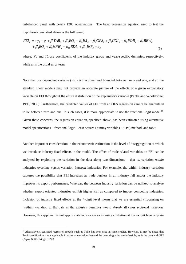
unbalanced panel with nearly 1200 observations. The basic regression equation used to test the

hypotheses described above is the following:

ititititit

ititititititittIit

INFRDINPWRO

REWFORCGIGPSIMEOTARFEI

111098

7654321

(1)

where, ϒI, and ϒt, are coefficients of the industry group and year-specific dummies, respectively,

while εit is the usual error term.

Note that our dependent variable (FEI) is fractional and bounded between zero and one, and so the

standard linear models may not provide an accurate picture of the effects of a given explanatory

variable on FEI throughout the entire distribution of the explanatory variable (Papke and Wooldridge,

1996, 2008). Furthermore, the predicted values of FEI from an OLS regression cannot be guaranteed

to lie between zero and one. In such cases, it is more appropriate to use the fractional logit model23

.

Given these concerns, the regression equation, specified above, has been estimated using alternative

model specifications – fractional logit, Least Square Dummy variable (LSDV) method, and tobit.

Another important consideration in the econometric estimation is the level of disaggregation at which

we introduce industry fixed effects in the model. The effect of trade related variables on FEI can be

analysed by exploiting the variation in the data along two dimensions – that is, variation within

industries overtime versus variation between industries. For example, the within industry variation

captures the possibility that FEI increases as trade barriers in an industry fall and/or the industry

improves its export performance. Whereas, the between industry variation can be utilized to analyse

whether export oriented industries exhibit higher FEI as compared to import competing industries.

Inclusion of industry fixed effects at the 4-digit level means that we are essentially focussing on

‘within’ variation in the data as the industry dummies would absorb all cross sectional variation.

However, this approach is not appropriate in our case as industry affiliation at the 4-digit level explain

23 Alternatively, censored regression models such as Tobit has been used in some studies. However, it may be noted that

Tobit specification is not applicable in cases where values beyond the censoring point are infeasible, as is the case with FEI

(Papke & Woolridge, 1996).

20

most of the variation in FEI24

. Once the 4-digit dummies are included, the model may not be able to

identify the impact of trade and technology related variables which, by their very nature, change

relatively slowly over time. Thus, our specification does not include 4-digit industry fixed effects as it

may defeat the very purpose of our analysis – that is, to study the impact of trade and technology

related industry characteristics on FEI. However, we have included industry group dummies at the 2-

digit ISIC level25

.

Data on employment, according to ISIC Rev 3 nomenclature, came from the UNIDO’s industrial

database, INDSTAT 4. Explanatory variables have been constructed using data from different sources

such as the UN-COMTRADE database, Annual Survey of Industries (ASI) from the Central

Statistical Organization (CSO), and Prowess database from the Centre for Monitoring Indian

Economy (CMIE). These sources provide data according to different commodity classification

systems. We have built a harmonised dataset by mapping the various classification systems with the

ISIC Rev 3 codes, the details of which is discussed in Appendix. Table A1, A3 and A4 in the

Appendix provide further details on variable construction, data sources, summary statistics and

correlation matrix of the variables included in the regression model. Overall, the correlation

coefficients among the explanatory variables are not very high except those between IM and EO

(0.6130) and RDI and FOR (0.5751). For the regression analysis, all explanatory variables in ratios

have been converted to percentages so as to make the coefficients of these variables comparable to

that of tariff rate, the latter being always defined in percentage terms.

6. Regression Results

Table 5 reports results of Fractional Logit and LSDV model specifications. The results from the Tobit

specifications have been reported in Table A5 in the Appendix. At the outset, it may be noted that

24 A regression analysis of FEI on 4-digit level industry dummies yield an adjusted R2 value of 0.8388. This means that

industry affiliation at the 4-digit level explain about 84% of the variation in FEI. 25 The amount of variation in FEI explained by membership in a particular 2-digit industry is much small since the adjusted

R2 for a regression using 21 dummy variables to control for the 22 industry groups at the 2-digit ISIC level is only 0.2870.

Inclusion of industry group dummies at the 2-digit level allows us to control for the influence of time invariant factors

operating at the relatively aggregate level of industrial grouping – for example, the influence of industry group associations.

21

different models give broadly similar results with respect to the signs and statistical significance of the

explanatory variables. For each model, the first five columns in Table 5 include industry group

dummies while the last column replaces these with factor-intensity dummies. These dummies are

included to control for time invariant sector specific effects on FEI.

The variable TARit is included to capture the cost-reduction effect of tariff reduction on FEI. We find

that this variable is negative and significant in all models giving credence to our hypothesis. In the

LSDV specification (see column 7), the estimated coefficient is -0.0002, which means that a 10

percentage point decline in tariff rates would increase the ratio of female to total employment by

0.002, which is not trivial given that the average value of FEI in our sample is only 0.068. The

corresponding fractional logit coefficient (see column 1) is larger (-0.0016) but the magnitude of the

coefficient is not directly comparable to the estimate from the LSDV model (Papke & Woolridge,

2008). However, the average marginal effects (AME) of the fractional logit regression can be

compared to the LSDV estimates and we find that the AME estimates, reported in Table 6, are similar

in magnitude to the LSDV estimates. Thus, firms tend to reduce costs by substituting male with

female workers as they are exposed to increased international competition through tariff reduction.

In order to gauge the importance of resource reallocation effect on FEI, we have included the

variables EOit, IMit and GPSit, all of which yield expected signs with statistical significance in most of

the specifications. We find that FEI is higher in industries characterized by higher export orientation

(EOit) and greater participation in global production sharing (GPSit). These results are consistent with

the argument that female workers are intensively employed in unskilled labour-intensive tasks, where

developing countries have comparative advantages. The magnitude of the coefficient in the LSDV

model suggests that a 10 percentage increase in EOit (percentage share of exports in output) would

increase FEI by about 0.007, a practically important effect (see column 7 in Table 5). For a similar

specification of the fractional logit model, the AME of EOit is about 0.006, which is comparable to the

LSDV estimate (see column 1 in Table 6).

22

Quantitatively, the effect of GPSit, the share of imported intermediates in total intermediate inputs,

appears even higher than that EOit. As expected, greater import penetration (IMit) exerts a negative

effect on FEI, which is consistent with the argument that import competing industries in developing

countries are skill and technology intensive and hence employ fewer female workers compared to

males. The magnitude of IMit’s coefficient is broadly comparable with that of EOit but, as expected,

with the opposite signs. Overall, these results imply that employment opportunities for women

workers in developing countries would increase to the extent trade liberalization leads to an expansion

of unskilled labour-intensive production activities in these countries.

The variables EOit and IMit are potentially collinear as we have noted a high degree of correlation

between them (see the correlation matrix in Appendix). Thus, we have run specifications by

alternatively dropping EOit and IMit and we find that the sign of these variables remain the same and

statistically significant (see columns 2, 3, 8 and 9 in Table 5). However, the point estimates turned out

to be smaller when we include only one of these variables compared to the specifications where we

include both. This is not surprising given that these variables exert opposite effects on the dependent

variable: while EOit is positively related to FEI, the other variable IMit exerts a negative effect. Thus,

due to the high degree of correlation between EOit and IMit, when only one of these variables is

included it could be capturing the effect of the excluded variable as well.

In order to examine the impact of new technology, we include the variables CGIit and FORit. The

variable representing the extent of multinational involvement (FORit.) yields statistically significant

negative coefficient in all specifications, which is consistent with the hypothesis that new technology

is biased against female workers. The variable representing capital goods import intensity (CGIit)

shows similar results in the LSDV regressions. This variable shows the expected negative coefficient

also in the fractional logit regression (see column 4 and 6) but not in all specifications26

. Overall,

these results suggest that use of newer technology creates a bias against female employment.

26 CGIit shows negative coefficient in the tobit specifications though not always statistically significant at the acceptable

level.

23

The variable measuring the intensity of R&D (RDIit) shows a significant negative coefficient in the

fractional logit specifications27

. The non-production worker ratio (NPWit), which is supposed to

control for the skill intensity of industries, is highly significant with the expected negative sign in all

specifications. The negative coefficients of skill and R&D variables provide further credence to the

view that employers prefer to employ men in technology-intensive tasks.

The logarithm of the variable ROit, representing real value of output, is negative and statistically

significant in most of the fractional logit specifications, which is in line with our observation, based

on descriptive data analysis, that female workers are increasingly getting concentrated in slow

growing industries while male employment growth is seen primarily in fast growing industries28

. The

fast growing industries in India are either skilled labour-intensive or capital-intensive but not the

traditional labour intensive industries (Panagariya, 2008). Thus, it is not surprising that, in contrast to

the experience of other developing countries, female employment has not increased significantly in

India under trade liberalization.

As expected, the variable REWit is negative and significant in all specifications indicating that a rise in

women’s relative wages would reduce their share in manufacturing employment. Finally, the variable

representing the degree of informalization in an industry (INFit) shows a significant negative

coefficient giving credence to the view that establishments are contracting out unskilled-labour

intensive and routine tasks where female workers are intensively employed. It has been argued that

India’s rigid labour laws create incentives for firms to minimize hiring of regular workers by resorting

to informalization. Our analysis shows that female workers disproportionately bear the burden of this

process as their jobs are becoming increasingly informal.

27 However, the variable RDIit fails to achieve statistical significance in the LSDV models when FORit is included as an

explanatory variable. This is due to the fact that these two variables are highly correlated (r = 0.58). RDIit always shows

statistical significance when FORit is dropped. 28 However, this variable is statistically indistinguishable from zero in LSDV and Tobit specifications (except in one of the

Tobit specifications where industry fixed effects are not included).

24

Insert Tables 5 and 6 here

7. Conclusion and Discussion

The employment effects of trade liberalization are not gender neutral and it can vary significantly

across industries. This paper analyses the role of different industry characteristics, in terms of trade

orientation, technology intensity and other factors, in determining female employment intensity (FEI)

in a panel of Indian manufacturing industries during 1998-2008, a period which witnessed significant

trade liberalization in India.

Our econometric analysis provides support for the hypothesis that tariff reduction would cause greater

employment opportunities for female workers as firms substitute male workers with low cost female

labour. We also find that the resource reallocation effect – that is, faster growth of unskilled labour

intensive industries, where India has a comparative advantage - contributes to female employment

growth. Further, greater participation in global production networks, along the lines of comparative

advantage, is found to increase FEI. By contrast, greater use of new technology and capital intensive

production would bias the gender composition of workforce against females.

Thus, trade liberalization can contribute positively or negatively towards overall female employment

depending on the relative importance of these opposing channels. While the cost reduction effect

resulting from heighted competitive pressure and resource reallocation effects stimulate greater

female employment, the technology channel works in the opposite direction. The fact that, at the

aggregate level, we fail to observe large growth of female employment in India’s organized

manufacturing during post liberalization period may imply that the negative technology effect may

have been offsetting the positive effects of trade liberalization on women’s employment.

The resource reallocation effect has not been strong enough to generate huge employment

opportunities for women at the aggregate level. This is consistent with the observation that the pattern

25

of India’s industrial specialization shows a fundamental disconnect with its relative endowments in

that despite being a labour-abundant country, India tends to specialize in capital and skill intensive

industries and services (Kochhar et al 2006; Panagariya, 2008; and Krueger, 2010). The fast growing

exports from the country are either skilled labour-intensive (such as drugs and pharmaceuticals and

fine chemicals) or capital-intensive (such as automobiles and parts). The share of capital-intensive

products in India’s manufacturing export basket more than doubled from about 23% in 1990 to nearly

54% in 2010 while the share of unskilled labour-intensive products nearly halved from 43% to 22%

(Veeramani, 2012). Due to its idiosyncratic specialization, India has also been locked out of the

vertically integrated global supply chains in manufacturing industries (Veeramani, 2013; Athukorala,

2014).

Thus, it is plausible to argue that the low growth of FEI in Indian industries is a consequence of

idiosyncrasies in the pattern of India’s industrial development. India’s industrial structure has been

built during the import substitution period by following a strategy which can be characterized as

‘comparative-advantage-defying’. While the earlier policy regime created a bias in favour of capital

and skill intensive manufacturing, the reforms since 1991 have not been comprehensive enough to

reduce, let alone remove, this bias. Though the post-1991 policy changes have gone a long way

toward product market liberalization by easing the entry barriers, the factor markets (labour and land)

are still plagued by severe distortions and policy induced rigidities. In particular, India’s archaic

labour laws create severe exit barriers and hence discourage large firms in manufacturing from

choosing labour-intensive activities and technologies (Panagariya, 2007). Trade liberalization by itself

does not guarantee specialization in line with the comparative advantage of a country if other policies

militate against the efficient pattern of resource allocation.

India’s labour laws, by encouraging capital-intensive production, provide an incentive to employ

relatively more male workers. It has also been noted that, due to rigid labour laws, there is

significant informalization of labour force in India’s formal manufacturing industries. Our

econometric analysis suggests that this process of informalisation has been occurring mainly at the

26

cost of regular employment for female workers. A flexible labour market, with appropriate social

safety nets, is a crucial necessary condition for the growth of formal manufacturing sector

employment for female workers in India.

References

Abraham, V. (2013). Missing Labour or consistent "De-Feminization"? Economic and Political

Weekly, 48(31), 99-108.

Aguayo-Tellez, E., Airola, J., & Juhn, C. (2010). Did trade liberalization help women? The case of

Mexico in the 1990s. NBER Working Paer Series, Working Paper 16195.

Aigner, D. J., & Cain, G. G. (1977). Statistical Theories of Discrimination in Labor Markets.

Industrial and Labour Relations Review, 30 (2), 175-187.

Arrow, K. J. (1973). The Theory of Discrimination. In O. Ashenfelter, & A. Rees (eds),

Discrimination in Labour Markets (pp. 3-33). N.J.: Princeton University Press.

Athukorala, P.-C. (2011). Production networks and trade patterns in East-Asia: Regionalization or

Globalization? Asian Economic Papers, 10(1), 65-95.

Athukorala, P.-C. (2014). How India fits into global production sharing: experience, prospects and

policy options. In India Policy Forum 2013-14, 10, Sage, India.

Barro, R. J., & Lee, J. W. (2013). A new set of educational attainment in the world, 1950-2010.

Journal of Development Economics, 104, 184-198.

Baslevent, C., & Onaran, O. (2004). The effect of export oriented growth on female labour market

outcomes in Turkey. World Devlopment, 32(8), 1375-1393.

Becker, G. (1957). The Economics of Discrimination. Chicago: University of Chicago Press.

27

Berik, G. (2005). Growth with Gender Inequity: Another look at East Asian Development. In Gender

Equalitty: striving for justice in an unequal world. UNRISD.

Bhalla, S. S., & Kaur, R. (2011). Labour Force Participation of Women in India: Some facts, some

queries. LSE Asia Research Centre, Working Paper 40.

Black, S. E., & Brainerd, E. (2004). Impoting equality? The impact of globalization on gender

discrimination. Industrial and Labor Relations Review, 57(4), 540-559.

Cagatay, N., & Berik, G. (1991). Transition to export-led growth in Turkey: is there a feminization of

employment? Capital and Class, 15(1), 153-177.

Cagatay, N., & Ozler, S. (1995, November). Feminization of the Labour Force: The Effects of Long-

Term Development and Structural Adjustment. World Development, 23(11), 1883-1894.

Chen, M. A., & Raveendran, G. (2012). Urban Employment in India: Recent Trends and Patterns.

Margin: The Journal of Applied Economic Research, 6(2), 159-179.

Chowdhury, S. (2011). Employment in India: what does the data show? Economic and Political

Weekly, 46(32), 23-26.

Chu, Y. W. (2002). Women and work in East Asia. Transforming Gender and Development in East

Asia, 61.

Duflo, E. (2012). Women Empowerment and Economic Development. Journal of Economic

Literature, 50(4), 1051-79.

Elson, D. (1999). Labour Markets as Gendered Institutions: Equality, Efficiency and Empowerment

Issues. World Development, 27(3), 611-627.

Erlat, G. (2000). Measuring the impact of trade flows on employment in the Turkish manufacturing

industry. Applied Economics, 32(9), 1169-1180.

28

Feenstra, R. (1998). Integration of trade and disintegration of production in the global economy.

Journal of Economic Perspectives, 12(4), 31-50.

Fontana, M. (2009). The Gender Effects of Trade Liberalization in Developing Countries: A Review

of the Literature. In M. Bussolo, & R. De Hoyos, Gender Aspects of the Trade and Poverty Nexus: A

Micro-Macro Approach. Palgrave Macmillan.

Hinloopen, J., & van Marrewijk, C. (2008). Empirical Trade Analysis (ETA) Center. Retrieved from

http://www2.econ.uu.nl/users/marrewijk/eta/intensity.htm

Hummels, D., Ishii, J., & Yi, K. M. (2001). The nature and growth of vertical specialization in world

trade. Journal of International Economics, 54(1), 75-96.

Joekes, S. (August, 1995). Trade related employment for women industry and services in developing

countries. Occasional Paper 5, UNDP, UNRISD, Geneva.

Kannan, K. P., & Raveendran, G. (2012). Counting and profiling the missing labour force. Economic

and Political Weekly, 47(6), 43-59.

Kapoor, R. (2014). Creating Jobs in India’s Organised Manufacturing Sector. ICRIER Working paper

(No. id: 6208).

Kim, T.H. and K.H. Kim, ``Industrial restructuring in Korea and it's consequences for women

workers,'' in Committee for Asian Women, Asian Women Workers Confront Challenges of Industrial

Restructuring. Research Papers and Consultation Recommendations on the Impact of Industrial

Restructuring on Women Workers in Asia (Hong Kong: Committee for Asian Women, 1995).

Kochhar, K., Kumar, U., Rajan, R., & Subramanium, A. (2006). India's psttern of development: what

happned, what follows? Journal of Monetary Economics, 53(5), 981-1019.

Korinek, J. (2005). Trade and Gender: issues and inteactions. OECD.

Krueger, A. O. (2010). Trade liberalization and growth in developing countries. In J. Siegfried, Better

living through economics. Harvard University Press

29

Krueger, A., Lary, H., & Monson, T. (1981). Trade and Employment in Developing Countries I:

individual studies. Chicago, University of Chicago Press.

Krusell, P., Ohanian, L. E., Rios-Rull, J.-V., & Violante, G. L. (2000). Capital-skill complementarity

and Inequlaity: a macroeconomic analysis. Econometrica, 68(5), 1029-1053.

Kucera, D., & Milberg, W. (2007). Gender segregation and gender bias in manufacturing trade

expansion. In I. v. Staveren, D. Elson, C. Grown, & N. Cagatay, The Feminist Economics of Trade

(pp. 185-214). Routledge.

Mazumdar, I., & Neetha, N. (2011). Gender Dimensions: Employment Trends in India 1993-94 to

2009-10. Economic and Political Weekly, 46(43), 118-126.

Mehra, R., & Gammage, S. (1999). Trends, countertrends, and gaps in women's employment. World

Development, 27(3), 533-550.

Milner, C., & Wright, P. (1998). Modelling labour market adjustment to trade liberalisation in an

industrialising economy. Economic Journal, 509-528.

Nordås, H. K. (2003). The impact of trade liberalization on women's job opportunities and earnings in

developing countries. World Trade Review, 2(02), 221-231

Ozler, S. (2000). Export orientation and female share of employment: evidence from Turkey. World

Devlopment, 28(7) 1239-1248.

Panagariya, A. (2007). Why India lags behind Chinda and How Can it Bridge the Gap. World

Economy, 30(2), 229-48.

Panagariya, A. (2008). India: The Emerging Giant. New York: Oxford University Press.

Papke, L. E., & Woolridge, J. M. (1996). Econometric Methods for Fractional Response Variables

with an Applicationto 401(k) Plan Participation Rates. Journal of Applied Econometrics, 11(6), 619-

632.

30

Papke, L. E., & Woolridge, J. M. (2008). Panel data methods for fractional response variables with an

application to test pass rates. Journal of Econometrics, 145(1), 121-133.

Pearson, R. (1998). Feminist visions of development research analysis and policy. London:

Routledge.

Pursell, G., Kishor, N., & Gupta, K. (2007). Manufacturing protection in India since independence.

In Australia South Asia Research Centre, Australian National University, paper presented at

conference August (pp. 20-21).

Rahman, R. I., & Islam, R. (2013). Female labour force participation in Bangaldesh: trends, drivers

and barriers. International Labour Organization.

Rangarajan, C., Iyer, P., & Kaul, S. (2011). Where is the missing labour force. Economic and

Political Weekly, 46(39), 39-71.

Rangarajan, C., Seema, & Vishesh, E. M. (2014). Developments in the workforce between 2009-10

and 2011-12. Economic and Political Weekly, 49(23), 117-121.

Saha, B., Sen, K., & Maiti, D. (2013). Trade openness, labour institutions and flexibilisation: Theory

and evidence from India. Labour Economics, 24, 180-195.

Srivastava, N., & Srivastava, R. (2010). Women, Work and Employment Outcomes in Rural India.

Economic and Political Weekly, 45(28), 49-63.

Standing, G. (1999). Global feminization through flexible labur: a theme revisited. World

Development, 27(3), 583-602.

Subramanian, A., & Roy, D. (2001). Who can explain the mauriritan miracle: Meade, Romer, Sachs

or Rodrik? IMF Working Paper.

Thomas, J. J. (2012). India's Labour Market During the 2000s. Economic and Political Weekly,

47(51).

31

United Nations. (2014). The Millennium Development Goals Report. New York: United Nations.

Veeramani, C. (2012). Anatomy of India's Merchandise Export Growth, 1993-94 to 2010-11.

Economic and Political Weekly, 47(1), 94-1014.

Veeramani, C. (2013). The 'Miracle' Still Waiting to Happen: Performance of India's Manufactured

Exports in Comparison to China. In M. S. Dev, India Development Report 2012-13 (pp. 132-150).

New Delhi: Oxford University Press.

Wood, A. (1991). North-South trade and female labour in manufacturing: an asymmetry. The Journal

of Development Studies, 27(2),168-189.

32

Tables

Table 1 : Distribution of Workers across Industry Groups (Percentage Shares)

Female Workers Male Workers Value Added Share

ISIC

Code Description 1999 2003 2008 1999 2003 2008 1999 2003 2008

15 Food and beverages 25.99 25.84 24.08 15.98 15.76 13.34 10.53 8.15 8.16

16 Tobacco products 10.50 12.09 5.64 5.44 5.54 4.04 2.11 2.09 1.60

17 Textiles 11.96 14.49 18.46 16.75 16.09 12.76 8.42 7.28 4.72

18 Wearing apparel, fur 18.29 20.78 22.65 2.02 2.93 3.86 1.95 1.56 1.70

19 Leather, leather products

and footwear 3.72 3.28 5.33 1.28 1.73 1.98 0.84 0.67 0.68

20 Wood products (excl.

furniture) 0.61 0.38 0.36 0.64 0.67 0.66 0.24 0.22 0.17

21 Paper and paper products 1.13 1.19 1.25 2.35 2.44 2.25 1.55 1.77 1.47

22 Printing and publishing 0.54 0.53 0.56 1.56 1.60 1.27 1.56 1.46 0.80

23 Coke, refined petroleum

products, nuclear fuel 0.22 0.17 0.15 0.99 1.08 1.16 3.48 11.80 13.12

24 Chemicals and chemical

products 12.07 9.03 7.76 10.14 9.83 9.11 22.94 18.04 15.61

25 Rubber and plastics

products 1.60 1.36 1.93 3.67 3.94 4.25 3.79 3.33 3.59

26 Non-metallic mineral

products 3.15 2.46 2.35 6.01 6.37 7.78 5.22 4.43 7.10

27 Basic metals 1.04 0.48 0.71 8.80 7.96 9.30 12.45 14.25 14.57

28 Fabricated metal products 0.64 0.49 0.65 3.89 4.09 5.18 2.47 2.44 3.38

29 Machinery and equipment

n.e.c. 0.66 0.54 0.71 6.56 5.81 7.78 6.04 5.19 7.70

30 Office, accounting and

computing machinery 0.38 0.22 0.16 0.20 0.29 0.19 0.28 0.80 0.33

31 Electrical machinery and

apparatus 1.34 1.25 1.51 3.33 3.08 3.41 3.64 3.12 4.03

32 Radio, television and

communication equipment 2.38 1.62 1.39 1.33 1.29 1.26 2.02 2.01 2.30

33 Medical, precision and

optical instruments 1.21 0.79 0.73 0.83 0.86 0.74 0.90 0.97 0.78

34 Motor vehicles, trailers,

semi-trailers 0.61 0.62 1.14 4.01 4.17 5.20 5.15 6.15 4.78

35 Other transport equipment 0.22 0.20 0.14 2.60 2.57 2.26 2.64 3.00 2.43

36 Miscellaneous

manufacturing 1.75 2.19 2.35 1.62 1.90 2.22 1.77 1.28 0.99

33

Table 2: Distribution of Workers across Trade Orientation and Facto-Intensity Based Industry Groups (Percentage

Shares)

Industry Groups

Female Workers Male Workers Value Added Share

1999 2003 2008 1999 2003 2008 1999 2003 2008

Exporting 81.23 85.26 86.38 72.51 73.94 73.22 64.20 69.42 68.58

Primary&Resource

Intensive 35.82 37.37 29.19 19.67 19.57 16.00 10.47 8.32 7.36

Unskilled Labour

Intensive 33.38 37.81 45.56 20.45 20.76 18.15 12.38 10.17 7.16

Capital Intensive 12.03 10.09 11.63 32.39 33.61 39.08 41.35 50.94 54.06

Import Competing 16.14 12.41 11.02 22.68 21.35 22.32 29.54 25.04 25.08

Primary&Resource

Intensive 2.18 1.79 1.74 5.09 5.17 4.82 4.25 4.30 4.65

Unskilled Labour

Intensive 0.26 0.22 0.30 0.26 0.28 0.43 0.13 0.20 0.18

Capital Intensive 13.70 10.40 8.98 17.33 15.90 17.07 25.15 20.54 20.25

Non Competing 2.63 2.33 2.60 4.81 4.71 4.46 6.26 5.54 6.34

Primary&Resource

Intensive 0.45 0.51 0.62 0.38 0.42 0.27 0.28 0.18 0.13

Unskilled Labour

Intensive 0.48 0.62 0.73 0.42 0.78 0.89 0.33 0.39 0.33

Capital Intensive 1.70 1.19 1.26 4.02 3.51 3.30 5.64 4.97 5.88

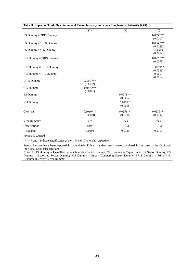
34

Table 3: Impact of Trade Orientation and Factor Intensity on Female Employment Intensity (FEI)

(1) (2) (3)

ES Dummy × PRIS Dummy

0.0655***

(0.0117)

ES Dummy × ULIS Dummy

0.0848***

(0.0129)

ES Dummy × CIS Dummy

-0.0089

(0.0054)

ICS Dummy × PRIS Dummy

0.0229***

(0.0078)

ICS Dummy × ULIS Dummy

0.0799**

(0.0336)

ICS Dummy × CIS Dummy

0.0065

(0.0062)

ULIS Dummy 0.0367***

(0.0137)

CIS Dummy -0.0479***

(0.0071)

ES Dummy

0.0271***

(0.0062)

ICS Dummy

0.0138**

(0.0058)

Constant 0.1010***

(0.0110)

0.0551***

(0.0108)

0.0539***

(0.0102)

Year Dummies Yes Yes Yes

Observations 1,193 1,193 1,193

R-squared 0.0980 0.0120 0.1110

Pseudo R-squared

***, ** and * indicate significance at the 1, 5 and 10% levels, respectively

Standard errors have been reported in parenthesis. Robust standard errors were calculated in the case of the OLS and

Fractional Logit specifications.

Notes: ULIS Dummy = Unskilled Labour Intensive Sector Dummy; CIS Dummy = Capital Intensive Sector Dummy; ES

Dummy = Exporting Sector Dummy; ICS Dummy = Import Competing Sector Dummy; PRIS Dummy = Primary &

Resource Intensive Sector Dummy

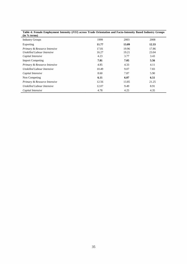
35

Table 4: Female Employment Intensity (FEI) across Trade Orientation and Facto-Intensity Based Industry Groups

(in % terms)

Industry Groups 1999 2003 2008

Exporting 11.77 13.09 12.33

Primary & Resource Intensive 17.81 19.96 17.86

Unskilled Labour Intensive 16.27 19.21 23.04

Capital Intensive 4.23 3.77 3.43

Import Competing 7.81 7.05 5.56

Primary & Resource Intensive 4.85 4.33 4.11

Unskilled Labour Intensive 10.49 9.07 7.83

Capital Intensive 8.60 7.87 5.90

Non Competing 6.11 6.07 6.51

Primary & Resource Intensive 12.56 13.85 21.25

Unskilled Labour Intensive 12.07 9.49 8.91

Capital Intensive 4.78 4.25 4.35

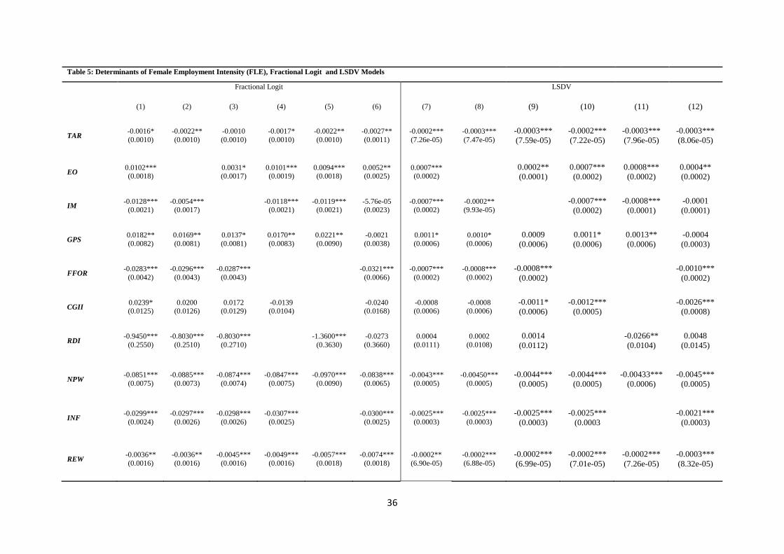
36

Table 5: Determinants of Female Employment Intensity (FLE), Fractional Logit and LSDV Models

Fractional Logit

LSDV

(1) (2) (3) (4) (5) (6) (7) (8) (9) (10) (11) (12)

TAR -0.0016*

(0.0010)

-0.0022**

(0.0010)

-0.0010

(0.0010)

-0.0017*

(0.0010)

-0.0022**

(0.0010)

-0.0027**

(0.0011)

-0.0002***

(7.26e-05)

-0.0003***

(7.47e-05)

-0.0003***

(7.59e-05)

-0.0002***

(7.22e-05)

-0.0003***

(7.96e-05)

-0.0003***

(8.06e-05)

EO 0.0102*** (0.0018)

0.0031* (0.0017)

0.0101*** (0.0019)

0.0094*** (0.0018)

0.0052** (0.0025)

0.0007*** (0.0002)

0.0002**

(0.0001)

0.0007***

(0.0002)

0.0008***

(0.0002)

0.0004**

(0.0002)

IM -0.0128***

(0.0021) -0.0054***

(0.0017) -0.0118***

(0.0021) -0.0119***

(0.0021) -5.76e-05 (0.0023)

-0.0007*** (0.0002)

-0.0002** (9.93e-05)

-0.0007***

(0.0002)

-0.0008***

(0.0001)

-0.0001

(0.0001)

GPS 0.0182**

(0.0082)

0.0169**

(0.0081)

0.0137*

(0.0081)

0.0170**

(0.0083)

0.0221**

(0.0090)

-0.0021

(0.0038)

0.0011*

(0.0006)

0.0010*

(0.0006)

0.0009

(0.0006)

0.0011*

(0.0006)

0.0013**

(0.0006)

-0.0004

(0.0003)

FFOR -0.0283***

(0.0042)

-0.0296***

(0.0043)

-0.0287***

(0.0043)

-0.0321***

(0.0066)

-0.0007***

(0.0002)

-0.0008***

(0.0002)

-0.0008***

(0.0002)

-0.0010***

(0.0002)

CGII 0.0239* (0.0125)

0.0200 (0.0126)

0.0172 (0.0129)

-0.0139 (0.0104)

-0.0240 (0.0168)

-0.0008 (0.0006)

-0.0008 (0.0006)

-0.0011*

(0.0006)

-0.0012***

(0.0005)

-0.0026***

(0.0008)

RDI -0.9450***

(0.2550)

-0.8030***

(0.2510)

-0.8030***

(0.2710)

-1.3600***

(0.3630)

-0.0273

(0.3660)

0.0004

(0.0111)

0.0002

(0.0108)

0.0014

(0.0112)

-0.0266**

(0.0104)

0.0048

(0.0145)

NPW -0.0851***

(0.0075)

-0.0885***

(0.0073)

-0.0874***

(0.0074)

-0.0847***

(0.0075)

-0.0970***

(0.0090)

-0.0838***

(0.0065)

-0.0043***

(0.0005)

-0.00450***

(0.0005)

-0.0044***

(0.0005)

-0.0044***

(0.0005)

-0.00433***

(0.0006)

-0.0045***

(0.0005)

INF -0.0299***

(0.0024)

-0.0297***

(0.0026)

-0.0298***

(0.0026)

-0.0307***

(0.0025)

-0.0300***

(0.0025)

-0.0025***

(0.0003)

-0.0025***

(0.0003)

-0.0025***

(0.0003)

-0.0025***

(0.0003

-0.0021***

(0.0003)

REW -0.0036**

(0.0016)

-0.0036**

(0.0016)

-0.0045***

(0.0016)

-0.0049***

(0.0016)

-0.0057***

(0.0018)

-0.0074***

(0.0018)

-0.0002**

(6.90e-05)

-0.0002***

(6.88e-05)

-0.0002***

(6.99e-05)

-0.0002***

(7.01e-05)

-0.0002***

(7.26e-05)

-0.0003***

(8.32e-05)

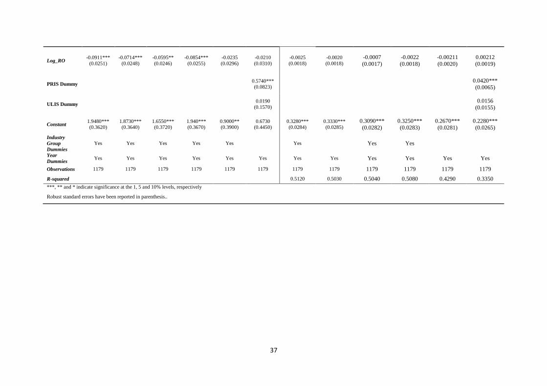
37

Log_RO -0.0911***

(0.0251)

-0.0714***

(0.0248)

-0.0595**

(0.0246)

-0.0854***

(0.0255)

-0.0235

(0.0296)

-0.0210

(0.0310)

-0.0025

(0.0018)

-0.0020

(0.0018)

-0.0007

(0.0017)

-0.0022

(0.0018)

-0.00211

(0.0020)

0.00212

(0.0019)

PRIS Dummy

0.5740*** (0.0823)

0.0420***

(0.0065)

ULIS Dummy

0.0190

(0.1570)

0.0156

(0.0155)

Constant 1.9480*** (0.3620)

1.8730*** (0.3640)

1.6550*** (0.3720)

1.940*** (0.3670)

0.9000** (0.3900)

0.6730 (0.4450)

0.3280*** (0.0284)

0.3330*** (0.0285)

0.3090***

(0.0282)

0.3250***

(0.0283)

0.2670***

(0.0281)

0.2280***

(0.0265)

Industry

Group

Dummies

Yes Yes Yes Yes Yes

Yes

Yes Yes

Year

Dummies Yes Yes Yes Yes Yes Yes Yes Yes Yes Yes Yes Yes

Observations 1179 1179 1179 1179 1179 1179 1179 1179 1179 1179 1179 1179

R-squared

0.5120 0.5030 0.5040 0.5080 0.4290 0.3350

***, ** and * indicate significance at the 1, 5 and 10% levels, respectively

Robust standard errors have been reported in parenthesis..

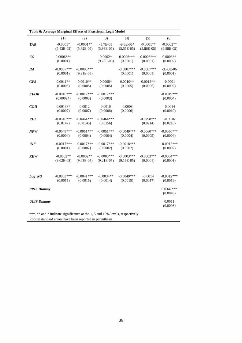
38

Table 6: Average Marginal Effects of Fractional Logit Model

(1) (2) (3) (4) (5) (6)

TAR -0.0001*

(5.43E-05)

-0.0001**

(5.82E-05)

-5.7E-05

(5.98E-05)

-9.6E-05*

(5.55E-05)

-0.0001**

(5.86E-05)

-0.0002**

(6.88E-05)

EO 0.0006***

(0.0001)

0.0002*

(9.78E-05)

0.0006***

(0.0001)

0.0006***

(0.0001)

0.0003**

(0.0002)

IM -0.0007***

(0.0001)

-0.0003***

(9.91E-05)

-0.0007***

(0.0001)

-0.0007***

(0.0001)

-3.43E-06

(0.0001)

GPS 0.0011**

(0.0005)

0.0010**

(0.0005)

0.0008*

(0.0005)

0.0010**

(0.0005)

0.0013**

(0.0005)

-0.0001

(0.0002)

FFOR -0.0016***

(0.00024)

-0.0017***

(0.0003)

-0.0017***

(0.0003)

-0.0019***

(0.0004)

CGII 0.00138*

(0.0007)

0.0012

(0.0007)

0.0010

(0.0008)

-0.0008

(0.0006)

-0.0014

(0.0010)

RDI -0.0545***

(0.0147)

-0.0464***

(0.0145)

-0.0464***

(0.0156)

-0.0798***

(0.0214)

-0.0016

(0.0218)

NPW -0.0049***

(0.0004)

-0.0051***

(0.0004)

-0.0051***

(0.0004)

-0.0049***

(0.0004)

-0.0060***

(0.0005)

-0.0050***

(0.0004)

INF -0.0017***

(0.0001)

-0.0017***

(0.0002)

-0.0017***

(0.0002)

-0.0018***

(0.0002)

-0.0012***

(0.0002)

REW -0.0002**

(9.02E-05)

-0.0002**

(9.05E-05)

-0.0003***

(9.21E-05)

-0.0003***

(9.16E-05)

-0.0003***

(0.0001)

-0.0004***

(0.0001)

Log_RO -0.0053***

(0.0015)

-0.0041***

(0.0015)

-0.0034**

(0.0014)

-0.0049***

(0.0015)

-0.0014

(0.0017)

-0.0012***

(0.0019)

PRIS Dummy 0.0342***

(0.0049)

ULIS Dummy 0.0011

(0.0093)

***, ** and * indicate significance at the 1, 5 and 10% levels, respectively

Robust standard errors have been reported in parenthesis.

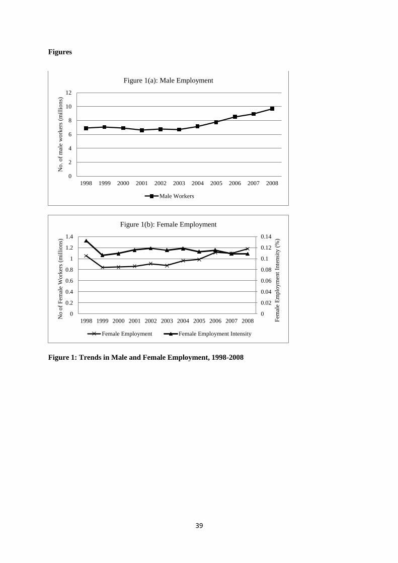
39

Figures

Figure 1: Trends in Male and Female Employment, 1998-2008

0

2

4

6

8

10

12

1998 1999 2000 2001 2002 2003 2004 2005 2006 2007 2008

No

. o

f m

ale

wo

rker

s (m

illi

on

s)

Figure 1(a): Male Employment

Male Workers

0

0.02

0.04

0.06

0.08

0.1

0.12

0.14

0

0.2

0.4

0.6

0.8

1

1.2

1.4

1998 1999 2000 2001 2002 2003 2004 2005 2006 2007 2008 Fem

ale

Em

plo

ym

ent

Inte

nsi

ty (

%)

No

of

Fem

ale

Wo

rker

s (m

illi

on

s)

Figure 1(b): Female Employment

Female Employment Female Employment Intensity

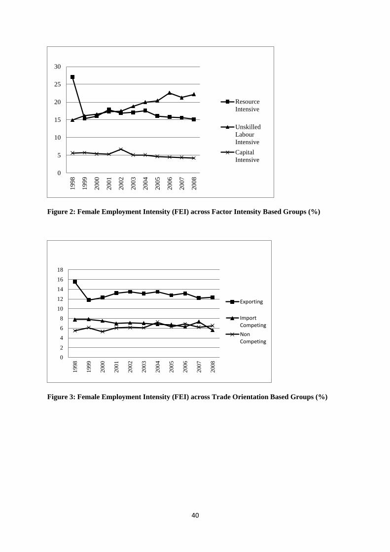
40

Figure 2: Female Employment Intensity (FEI) across Factor Intensity Based Groups (%)

Figure 3: Female Employment Intensity (FEI) across Trade Orientation Based Groups (%)

0

5

10

15

20

25

301

99

8

199

9

200

0

200

1

200

2

200

3

200

4

200

5

200

6

200

7

200

8

Resource

Intensive

Unskilled

Labour

Intensive

Capital

Intensive

0

2

4

6

8

10

12

14

16

18

199

8

199

9

200

0

200

1

200

2

200

3

200

4

200

5

200

6

200

7

200

8

Exporting

ImportCompeting

NonCompeting

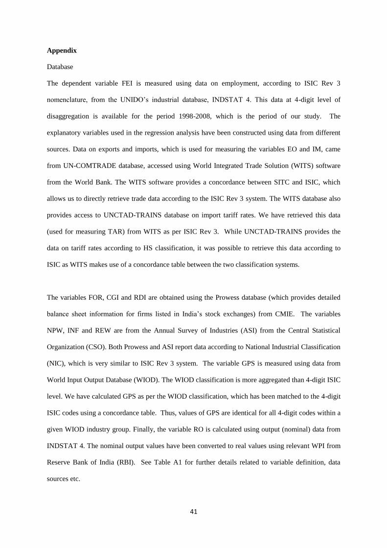
41

Appendix

Database

The dependent variable FEI is measured using data on employment, according to ISIC Rev 3

nomenclature, from the UNIDO’s industrial database, INDSTAT 4. This data at 4-digit level of

disaggregation is available for the period 1998-2008, which is the period of our study. The

explanatory variables used in the regression analysis have been constructed using data from different

sources. Data on exports and imports, which is used for measuring the variables EO and IM, came

from UN-COMTRADE database, accessed using World Integrated Trade Solution (WITS) software

from the World Bank. The WITS software provides a concordance between SITC and ISIC, which

allows us to directly retrieve trade data according to the ISIC Rev 3 system. The WITS database also

provides access to UNCTAD-TRAINS database on import tariff rates. We have retrieved this data

(used for measuring TAR) from WITS as per ISIC Rev 3. While UNCTAD-TRAINS provides the

data on tariff rates according to HS classification, it was possible to retrieve this data according to

ISIC as WITS makes use of a concordance table between the two classification systems.

The variables FOR, CGI and RDI are obtained using the Prowess database (which provides detailed

balance sheet information for firms listed in India’s stock exchanges) from CMIE. The variables

NPW, INF and REW are from the Annual Survey of Industries (ASI) from the Central Statistical

Organization (CSO). Both Prowess and ASI report data according to National Industrial Classification

(NIC), which is very similar to ISIC Rev 3 system. The variable GPS is measured using data from

World Input Output Database (WIOD). The WIOD classification is more aggregated than 4-digit ISIC

level. We have calculated GPS as per the WIOD classification, which has been matched to the 4-digit

ISIC codes using a concordance table. Thus, values of GPS are identical for all 4-digit codes within a

given WIOD industry group. Finally, the variable RO is calculated using output (nominal) data from

INDSTAT 4. The nominal output values have been converted to real values using relevant WPI from

Reserve Bank of India (RBI). See Table A1 for further details related to variable definition, data

sources etc.

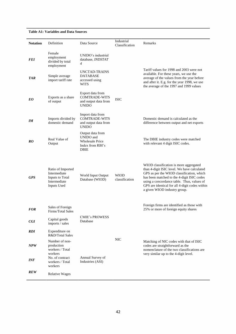
42

Table A1: Variables and Data Sources

Notation Definition Data Source Industrial

Classification Remarks

FEI

Female

employment

divided by total

employment

UNIDO’s industrial

database, INDSTAT

4

ISIC

TAR Simple average

import tariff rate

UNCTAD-TRAINS

DATABASE

accessed using

WITS

Tariff values for 1998 and 2003 were not

available. For these years, we use the

average of the values from the year before

and after it. E.g. for the year 1998, we use

the average of the 1997 and 1999 values

EO Exports as a share

of output

Export data from

COMTRADE-WITS

and output data from

UNIDO

IM Imports divided by

domestic demand

Import data from

COMTRADE-WITS

and output data from

UNIDO

Domestic demand is calculated as the

difference between output and net exports

RO Real Value of

Output

Output data from

UNIDO and

Wholesale Price

Index from RBI’s

DBIE

The DBIE industry codes were matched

with relevant 4 digit ISIC codes.

GPS

Ratio of Imported

Intermediate

Inputs to Total

Intermediate

Inputs Used

World Input Output

Database (WIOD)

WIOD

classification

WIOD classification is more aggregated

than 4-digit ISIC level. We have calculated

GPS as per the WIOD classification, which

has been matched to the 4-digit ISIC codes

using a concordance table. Thus, values of

GPS are identical for all 4-digit codes within

a given WIOD industry group.

FOR Sales of Foreign

Firms/Total Sales

CMIE’s PROWESS

Database

NIC

Foreign firms are identified as those with

25% or more of foreign equity shares

CGI Capital goods

imports / sales

Matching of NIC codes with that of ISIC

codes are straightforward as the

nomenclature of the two classifications are

very similar up to the 4-digit level.

RDI Expenditure on

R&D/Total Sales

NPW

Number of non-

production

workers / Total

workers Annual Survey of

Industries (ASI) INF

No. of contract

workers / Total

workers

REW Relative Wages

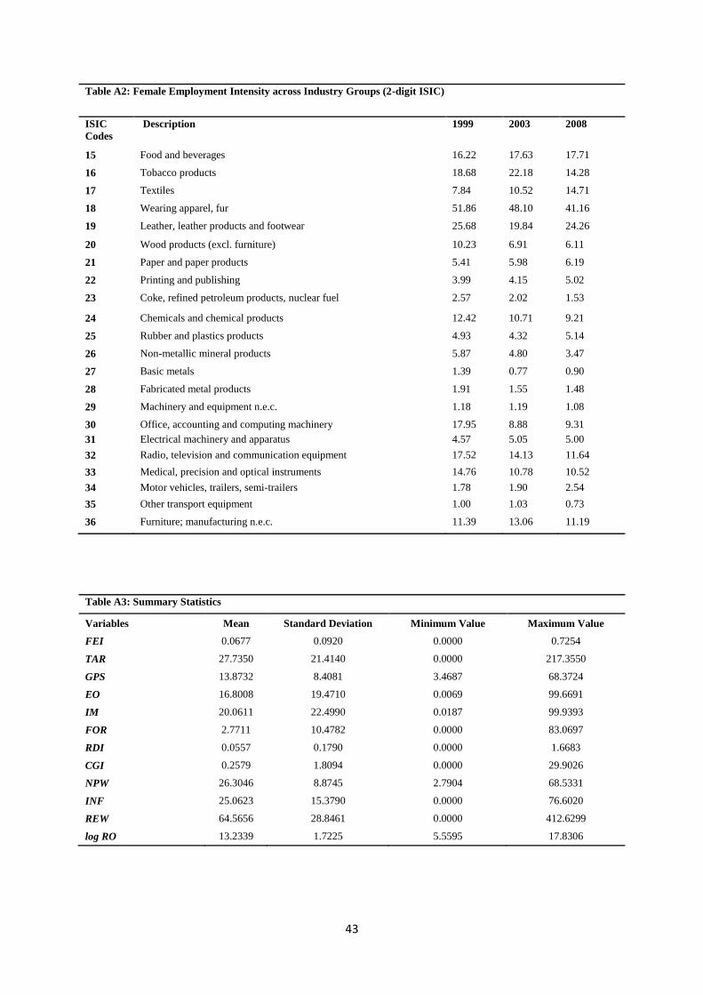
43

Table A2: Female Employment Intensity across Industry Groups (2-digit ISIC)

ISIC

Codes

Description 1999

2003

2008

15 Food and beverages 16.22 17.63 17.71

16 Tobacco products 18.68 22.18 14.28

17 Textiles 7.84 10.52 14.71

18 Wearing apparel, fur 51.86 48.10 41.16

19 Leather, leather products and footwear 25.68 19.84 24.26

20 Wood products (excl. furniture) 10.23 6.91 6.11

21 Paper and paper products 5.41 5.98 6.19

22 Printing and publishing 3.99 4.15 5.02

23 Coke, refined petroleum products, nuclear fuel 2.57 2.02 1.53

24 Chemicals and chemical products 12.42 10.71 9.21

25 Rubber and plastics products 4.93 4.32 5.14

26 Non-metallic mineral products 5.87 4.80 3.47

27 Basic metals 1.39 0.77 0.90

28 Fabricated metal products 1.91 1.55 1.48

29 Machinery and equipment n.e.c. 1.18 1.19 1.08

30 Office, accounting and computing machinery 17.95 8.88 9.31

31 Electrical machinery and apparatus 4.57 5.05 5.00

32 Radio, television and communication equipment 17.52 14.13 11.64

33 Medical, precision and optical instruments 14.76 10.78 10.52

34 Motor vehicles, trailers, semi-trailers 1.78 1.90 2.54

35 Other transport equipment 1.00 1.03 0.73

36 Furniture; manufacturing n.e.c. 11.39 13.06 11.19

Table A3: Summary Statistics

Variables Mean Standard Deviation Minimum Value Maximum Value

FEI 0.0677 0.0920 0.0000 0.7254

TAR 27.7350 21.4140 0.0000 217.3550

GPS 13.8732 8.4081 3.4687 68.3724

EO 16.8008 19.4710 0.0069 99.6691

IM 20.0611 22.4990 0.0187 99.9393

FOR 2.7711 10.4782 0.0000 83.0697

RDI 0.0557 0.1790 0.0000 1.6683

CGI 0.2579 1.8094 0.0000 29.9026

NPW 26.3046 8.8745 2.7904 68.5331

INF 25.0623 15.3790 0.0000 76.6020

REW 64.5656 28.8461 0.0000 412.6299

log RO 13.2339 1.7225 5.5595 17.8306

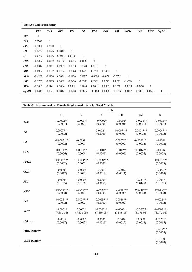
44

Table A4: Correlation Matrix

FEI TAR GPS EO IM FOR CGI RDI NPW INF REW log RO

FEI 1

TAR 0.0560 1

GPS -0.1080 -0.3200 1

EO 0.1275 -0.1925 0.0840 1

IM -0.0762 -0.2886 0.1945 0.6130 1

FOR -0.1362 -0.0390 0.0177 -0.0915 -0.0528 1

CGI -0.0342 -0.0161 0.0958 -0.0018 0.0028 0.1165 1

RDI -0.0992 -0.0532 0.0154 -0.0563 -0.0476 0.5751 0.3423 1

NPW -0.4209 -0.1168 0.0094 -0.1153 0.1997 -0.0004 -0.072 -0.0052 1

INF -0.1759 -0.0113 0.1037 -0.0455 -0.1306 0.0959 0.0245 0.0706 -0.2712 1

REW -0.1669 -0.1441 0.1084 0.0002 0.1420 0.1663 0.0395 0.1721 0.0919 -0.0276 1

log RO -0.0411 -0.0521 0.0842 -0.1233 -0.1817 -0.1183 0.0096 -0.0816 0.0137 0.1856 0.0555 1

Table A5: Determinants of Female Employment Intensity: Tobit Models

Tobit

(1) (2) (3) (4) (5) (6)

TAR -0.0002**

(0.0001)

-0.0003**

(0.0001)

-0.0002*

(0.0001)

-0.0002*

(0.0001)

-0.0025**

(0.0001)

-0.0003**

(0.0001)

EO 0.0007***

(0.0002)

0.0002**

(0.0001)

0.0007***

(0.0002)

0.0008***

(0.0002)

0.0004***

(0.0002)

IM -0.0007***

(0.0002)

-0.0002*

(0.0001)

-0.0007***

(0.0002)

-0.0008***

(0.0002)

-0.0001

(0.0002)

GPS 0.0011**

(0.0006)

0.0011**

(0.0006)

0.0010*

(0.0006)

0.0012**

(0.0006)

0.0014**

(0.0006)

-0.0004

(0.0003)

FFOR -0.0007***

(0.0002)

-0.0008***

(0.0003)

-0.0008***

(0.0003)

-0.0010***

(0.0003)

CGII -0.0008

(0.0012)

-0.0008

(0.0012)

-0.0011

(0.0012)

-0.0013

(0.0011)

-0.0027*

(0.0014)

RDI -0.0005

(0.0155)

-0.0007

(0.0156)

0.0005

(0.0156)

-0.0274*

(0.0145)

0.0057

(0.0161)

NPW -0.0045***

(0.0003)

-0.0046***

(0.0003)

-0.0046***

(0.0004)

-0.0045***

(0.0003)

-0.0045***

(0.0003)

-0.0050***

(0.0003)

INF -0.0025***

(0.0002)

-0.0025***

(0.0002)

-0.0025***

(0.0002)

-0.0026***

(0.0002)

-0.0021***

(0.0002)

REW -0.0001*

(7.58e-05)

-0.0002**

(7.63e-05)

-0.0002**

(7.63e-05)

-0.0002**

(7.54e-05)

-0.0002*

(8.17e-05)

-0.0003***

(8.17e-05)

Log_RO -0.0012

(0.0017)

-0.0007

(0.0017)

0.0006

(0.0016)

-0.0010

(0.0017)

-0.0007

(0.0018)

0.0029**

(0.0015)

PRIS Dummy

0.0433***

(0.0064)

ULIS Dummy

0.0159

(0.0098)

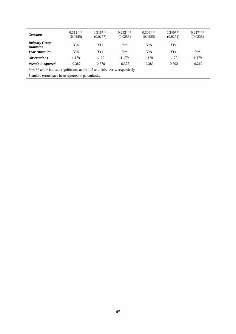
45

Constant 0.312***

(0.0255)

0.316***

(0.0257)

0.292***

(0.0253)

0.309***

(0.0255)

0.249***

(0.0272)

0.217***

(0.0238)

Industry Group

Dummies Yes Yes Yes Yes Yes

Year Dummies Yes Yes Yes Yes Yes Yes

Observations 1,179 1,179 1,179 1,179 1,179 1,179

Pseudo R-squared -0.387 -0.378 -0.378 -0.383 -0.302 -0.219

***, ** and * indicate significance at the 1, 5 and 10% levels, respectively

Standard errors have been reported in parenthesis.