Trade in Intermediate Inputsand Business Cycle Comovement

Robert C. Johnson∗

First Draft: October 2010This Draft: June 2011

Abstract

In data, bilateral trade is strongly correlated with bilateral GDP comovement.This paper examines whether trade in intermediate inputs explains this empirical fact.I integrate input trade into a many country, multi-sector model and calibrate themodel to data on bilateral input-output linkages. With estimated productivity shocks,the model generates an aggregate trade-comovement correlation 30-40% as large asin data. This moderate aggregate correlation emerges because the model matchesobserved correlations of goods production well, but fails to match services correlations.With independent shocks across countries, the model accounts for one-quarter of thetrade-comovement relationship for gross output of goods. However, because shocks aretransmitted through input linkages, they synchronize gross output, not value added.Moreover, contrary to conventional wisdom, input complementarity does not reconcilemodel and data. Finally, using simulated data, I argue that caution is needed ininterpreting trade-comovement regressions that include proxies for vertical linkages.

∗Economics Department, Dartmouth College, robert.c.johnson@dartmouth.edu. I thank RudolfsBems, Andrew Bernard, Stefania Garetto, Jean Imbs, Luciana Juvenal, Esteban Rossi-Hansberg, Nina Pavc-nik, and Kei-Mu Yi for helpful conversations, as well as participants in presentations at the Dallas FederalReserve, Johns Hopkins (SAIS), Penn State, Stanford, the St. Louis Federal Reserve, UC Santa Cruz, the2011 AEA meetings, and the 2010 EIIT Conference.

1

1 Introduction

A large empirical literature suggests that international trade transmits shocks and synchro-

nizes economic activity across borders. For example, bilateral trade is strongly (and robustly)

correlated with bilateral GDP comovement.1 Though standard international real business

cycle (IRBC) models predict a positive correlation between trade and comovement, they

cannot replicate the quantitative magnitude of the empirical correlation. For example, Kose

and Yi (2006) show that the change in bilateral comovement generated by an exogenous

change in bilateral trade intensity is at most one-tenth the size of the partial correlation

between trade and comovement observed in the data. They have dubbed this the “trade

comovement puzzle.”

In addressing this puzzle, recent empirical work has turned attention to the role of inter-

mediate goods trade as a conduit for shocks. For example, Ng (2010) documents that proxies

for bilateral production fragmentation predict bilateral GDP correlations, while Di Giovanni

and Levchenko (2010) document that bilateral trade is more important in explaining output

comovement for home and foreign sectors that use each other as intermediates. Further,

Burstein, Kurz, and Tesar (2008) show that countries that intensively engage in intra-firm

trade with United States multinational parents display higher manufacturing output corre-

lations with the U.S.2

This focus on input trade is potentially important, since intermediate inputs account

for roughly two-thirds of international trade. To examine the role of input trade in shock

propagation, I develop a many country, multi-sector extension of the standard international

real business cycles model with trade in both intermediate and final goods. I then calibrate

the model to data on bilateral final and intermediate goods trade flows for 22 countries and a

composite rest-of-the-world region, and simulate model responses to sector-specific produc-

tivity shocks. Using simulated data, I assess the ability of the model with intermediates to

explain observed bilateral output correlations, highlighting the role of input trade in driving

comovement.

In the model, input trade transmits shocks across borders independent of, and in addition

to, standard IRBC transmission mechanisms. In the cannonical model, idiosyncratic shocks

generate output comovement by inducing comovement in factor supplies. Specifically, a

positive shock in the home country raises home output and depreciates home’s terms of

1See, for example, Frankel and Rose (1998), Imbs (2004), Baxter and Kouparitsas (2005), Kose andYi (2005), Calderon, Chong, and Stein (2007), Inklaar, Jong-A-Pin, and Haan (2008), Di Giovanni andLevchenko (2010), and Ng (2010).

2In a related vein, Bergin, Feenstra, and Hanson (2009) find that Mexican export assembly (maquiladora)industries are twice as volatile as their US counterparts, suggesting possibly strong transmission of US shocksto Mexico via production sharing linkages.

2

trade, which induces increased factor supply and hence output abroad.3 This mechanism

continues to operate in the augmented model with intermediate inputs. However, with

traded intermediates, productivity shocks are passed downstream through the production

chain directly.4 One implication of this is that input linkages generate comovement in gross

output even if factor supply is exogenous, which in turn implies that comovement in gross

output may be delinked from comovement in real value added. Thus, the production chain

puts significant additional structure to how shocks are transmitted.

To evaluate these channels quantitatively, I calibrate the model to data on bilateral final

and intermediate goods trade. Following Johnson and Noguera (2010), I use data from

national input-output tables combined with data on bilateral trade to construct a synthetic

global input-output framework. This framework describes how individual sectors in each

country source intermediate goods from both home and bilateral import sources, as well

as how each country sources final goods. This data has several advantageous features for

calibration of international macro models. First, the framework respects national accounts

definitions of final and intermediate goods, and therefore is consistent with standard macro

aggregates. Second, the framework explicitly accounts for the “double counting” problem in

gross trade statistics, wherein the gross exports exceeds the value added content of exports.

These features provide for a more realistic calibration of openness and bilateral linkages than

has been previously possible in the literature.

Proceeding to the numerical analysis, I first simulate the model using an estimated pro-

ductivity process in which shocks are allowed to be correlated across countries, as in the data.

This model generates an aggregate trade-comovement correlation 30-40% the size of the ob-

served correlation. Disaggregating this result, the model generates strong cross-country

correlations for goods, but not for services. For example, a trade-comovement regression

for gross output of goods returns a coefficient roughly 3/4 the size of the correlation in the

data, as compared to a correlation for services that is insignificantly different from zero. The

aggregate trade-comovement coefficient then lies between these extremes, which implies that

generating higher aggregate comovement from the model requires modifying the model in

ways that raise the correlation of services.

These initial results represent an upper bound on the role of trade in propagating shocks,

as they they confound the effects of idiosyncratic shock propagation with the correlation of

3Several recent papers strenthen this mechanism by lowering the short run elasticity of substitutionbetween home and foreign goods, for example by introducing durable goods (Engel and Wang (2011)) orsearch and matching frictions (Drozad and Nosal (2008)).

4Productivity shocks travel unidirectionally downstream when intermediate goods are aggregated in aCobb-Douglas fashion, the case considered in the benchmark model below. More generally, productivityshocks travel both downstream to input users and upstream to input suppliers.

3

shocks across countries themselves. To isolate the propagation mechanism, I simulate the

model again using shocks that are uncorrelated across countries. In these simulations, the

trade-comovement correlation falls substantially for real value added, both in the aggregate

and at the sector level. This implies that the correlation of shocks across countries is primarily

responsible for value added comovement.

Interestingly however, there is significant propagation of idiosyncratic shocks for gross

output. For gross output, idiosyncratic shocks account for roughly one-quarter of the trade-

comovement correlation in the data. This discrepancy between the comovement in real

value added versus intermediate goods points to the role of intermediates in the model.

Specifically, gross output in the model is a composite of real value added and intermediate

inputs. Therefore, gross output can be correlated across countries either because real value

added is correlated, or because intermediate use is correlated. In the model, comovement

following idiosyncratic shocks is primarily due to comovement in intermediate use. This is

because intermediate trade is the primary conduit through which shocks travel in the model.

Using this framework, I explore whether complementarity of intermediates amplifies co-

movement. I introduce complementarity in two different ways: first making intermediates

complements among themselves, and second making intermediates complementary with non-

produced factor inputs (i.e., capital and labor). Contrary to conventional wisdom, comple-

mentarity fails to narrow the gap between the model and data in both cases. Complemen-

tarity within the input bundle raises output comovement dramatically, but does not amplify

real value added comovement. Complementarity between intermediates and factor inputs

constrains fluctuations in demand for intermediates, thereby lowering comovement in gross

output.

Finally, one advantage to simulating a many country model is that I generate an en-

tire data set similar to those used in empirical work. To exploit this, I use my simulated

data to examine whether trade-comovement regressions that control for ‘vertical linkages’

or cross-border ‘fragmentation’ are capable of cleanly identifying the role of intermediates

in generating comovement. I argue that coefficients on proxies for production sharing in

trade-comovement regressions are difficult to interpret, as they appear to be correlated with

omitted shocks driving output correlations.

In addition to the empirical work cited above, this paper is related to a number of

recent attempts to incorporate production sharing into business cycle models. The closest

antecedent to the model developed below is a two-country, two-sector IRBC model with

intermediates by Ambler, Cardia, and Zimmerman (2002).5 This paper is distinguished

5Both Ambler et al. and this paper are also related to Cole and Obstfeld (1991) who write down a twocountry model with intermediate linkages and full depreciation of capital in the spirit of Long and Plosser

4

from Amber et al. in both scope and focus. Whereas Amber et al. focus on a stylized two

country case, I calibrate and simulate a many country model to match data on bilateral

production sharing relations. Further, I hone the empirical focus toward understanding the

trade-comovement puzzle, in contrast to the focus on general business cycle properties of

the model in Ambler et al. Lastly, my exposition and analysis of the basic mechanisms

underlying international comovement differs substantially from Ambler et al.6

This paper is also related in spirit to recent models by Burstein, Kurz, and Tesar (2008)

and Arkolakis and Ramanarayan (2009). Burstein, Kurz, and Tesar (2008) specify a two sec-

tor IRBC model in which the production sharing sector has a lower elasticity of substitution

between home and foreign goods than the non-production sharing sector, which effectively

lowers the aggregate elasticity of substitution and raises comovement.7 Arkolakis and Ra-

manarayan (2009) adopt a multi-stage production function, an approach that is significantly

different and less tractable in a multi-country setting than the approach in this paper.

More broadly, the basic structure of the model in this paper has important characteris-

tics in common with models of sectoral linkages within the domestic economy, such as those

analyzed by Long and Plosser (1983), Horvath (1998, 2000), Dupor (1999), Shea (2002), Car-

valho (2008), or Foerster, Sarte, and Watson (2011). These papers provide many insights

into the role input-linkages play in translating idiosyncratic shocks into aggregate fluctua-

tions that could be applied to understanding regional business cycles using the framework

and data introduced below. However, there is an important difference to keep in mind.

Within the domestic economy, factors may be reallocated across sectors following a shock,

whereas factors are comparatively immobile across countries in the international framework

considered below.

Finally, in simulating a international macro model with more than two heterogeneous

countries, the paper is also related to work by Zimmerman (1997), Kose and Yi (2006),

Ishise (2009, 2010), and Juvenal and Monteiro (2010). These papers emphasize that third-

country effects may be important in driving bilateral correlations, effects that are picked up

in my many country framework. None feature trade in inputs, however.

(1983). This seems to be an under-appreciated contribution of their paper.6Ambler et al. devote attention to analyzing the role of investment frictions in their framework and

explaining the differences between their empirical findings and those of Long and Plosser (1983) by appealingto different assumptions regarding capital depreciation.

7In contrast to the model in this paper, the performance of the Burstein et al. model is identical regardlessof whether they assume that goods cross borders only once or whether there is back-and-forth shipment ofgoods across the border associated with production sharing.

5

2 Mechanics of Output Comovement

I begin by articulating a stylized static model that isolates some key features of the full

dynamic model. The general formulation of the static model combines international trade in

both final and intermediate goods with endogenous factor supply. This framework nests two

separate channels for transmitting shocks across borders and generating output comovement.

To develop intuition, I compare two polar opposite cases of the framework that clearly

separate the two channels.

In the first case, I assume that there is no trade in intermediate goods. This case cor-

responds to the static version of the standard multi-good international real business cycle

model, in which comovement is driven by endogenous factor supply.8 In the second case,

I assume that there is no trade in final goods and that factor supply is exogenous. This

case isolates the role of intermediate goods linkages in generating output comovement, and

highlights an important distinction between comovement in gross output versus value added.

2.1 A Benchmark Model

Consider a static world economy with many countries (i, j ∈ {1, . . . , N}). Country i produces

a single tradable Armington differentiated good using labor Li and composite intermediate

good Xi, which is a CES aggregate of intermediate goods produced by different source

countries. The aggregate production function is Cobb-Douglas in the domestic factor and

the composite intermediate:

Qi = Zi (Xi)θ L1−θ

i

with Xi =

(∑j

ωxjiXρji

)1/ρ

,(1)

where Xi is a CES aggregate of intermediate inputs produced in j and shipped to i (with

technology weights ωxji), θ is the intermediate input share in production, and Zi is exogenous

productivity.

Each country is populated by a representative consumer. The consumer is endowed with

8See Backus, Kehoe, and Kydland (1994) or Baxter (1995).

6

labor that it supplies to firms and consumes final goods. The consumer has preferences:

Ui(Ci, Li) = log(Ci)−χε

1 + εL

(1+ε)/εi

with Ci =

(∑j

ωcjiCγji

)1/γ

,(2)

where Ci is a CES aggregate of final goods produced in j and shipped to i (with preference

weights ωcji), χ measures the disutility of working, and ε is the Frisch elasticity of labor

supply.

For simplicity, I assume there exists a social planner.9 The planner maximizes a so-

cial welfare function that is the weighted sum of utility of consumers from each country:∑i µiUi(Ci, Li), where µi is the welfare weight assigned to the consumer in country i. The

social planner is constrained by the following adding-up condition for output from each coun-

try: Qi =∑

j Cij +Xij. This states that output in each country equals the sum of shipments

of final and intermediate goods from country i to all destinations j.

The social planners problem is then to choose {{Cji, Xji}∀j, Li}∀i to solve:

max∑i

µi

[log(Ci)−

χε

1 + εL

(1+ε)/εi

]s.t. Qi = Zi (Xi)

θ L1−θi

and Qi =∑j

Cij +Xij,

(3)

where Ci and Xi are defined above.

The production structure here differs in an important way from the standard IRBC

framework.10 The standard framework does not admit multi-stage, vertically specialized

production processes in which imports are used to produce exports. In contrast, the produc-

tion function and resource constraints above represent a multi-stage production process with

an effectively infinite number of production stages, where value is added at each stage in

a decreasing geometric sequence. Because production requires both domestic and imported

intermediates, gross trade will be a multiple over actual value exchanged between countries,

9I elect to have a social planner here for expositional simplicity. No result depends on this assumption.Moreover, in Section 2.3, I discuss the mechanics of the model in a case with Cobb-Douglas preferences andtechnologies, which implies that perfect risk sharing obtains through terms of trade effects even without theexistence of a social planner.

10Some semantic confusion may arise in comparing these frameworks. Starting at least with Backus,Kehoe, and Kydland (1994), IRBC models typically talk about trade in “intermediate goods,” which areaggregated to produce a “composite final good.” Despite this nomenclature, trade in these models shouldbe thought of as trade in quasi-final goods, wherein each good crosses an international border only once.

7

as goods cross borders many times throughout the production process. In contrast, the

domestic value added content of exports is equal to one in the standard framework.

2.2 Case One: No Intermediate Goods Trade

To mimic the IRBC framework, I assume here that there are no intermediate goods in the

model, setting θ = 0, which necessarily eliminates trade in intermediates.11 In this event,

the production function is linear in labor: Qi = ZiLi. As such, if productivity innovations

are independent across countries, output in country i is correlated with output in country j

only if factor supplies Li and Lj co-move.

To understand when these factor supplies co-move, we can turn to the first-order condi-

tions for the social planners problem in this case. Using the first-order condition for labor,

we can write factor supply in country i as:

Li =

(λiZiχµi

)ε, (4)

where λi is the shadow price of output in country i. Labor supply here is increasing in

productivity and the shadow price of output in country i, as both raise the marginal revenue

product of labor. Using the production function, then output can be written as:

Qi = Z1+εi λεi(χµi)

−ε. (5)

Given a productivity innovation in country i, the resulting change in output is given by:

Qi = (1 + ε)Zi + ελi. (6)

Obviously, the shadow price of output λi itself depends on productivity, but this formulation

is instructive because it highlights three channels for understanding the effect of productivity

on output. First, a productivity shock directly raises output. Second, a productivity shock

raises the amount of labor supplied, holding the output price fixed. Third, a productivity

shock will tend to drive down the shadow price of output (λi), which will attenuate the

amount by which labor supply (and hence output) rises.

In this formulation, a productivity shock spills across borders via relative prices. As

productivity rises in country i, the relative price of output in country i falls, equivalently the

relative price of output in country j rises. As the relative price of output in country j rises,

11A natural alternative assumption would be that each country uses only its own good as an intermediate.This yields similar results to assuming that there are no intermediates in the model.

8

this induces the representative consumer in j to supply more labor, which raises country j’s

output. Thus, output in country i rises due to the direct effect of productivity on output

and the indirect effect of productivity in raising labor supply, while output in country j rises

because terms of trade movements raise the return to supplying labor.

In this version of model, endogenous factor supply is the basic mechanism that drives

comovement, as in IRBC models more generally.12 The strength with which productivity

shocks spill across borders then depends on: (a) how responsive relative prices are to the

underlying shocks; (b) the elasticity of factor supply. In the extreme, when labor supply

is inelastic and productivity shocks are independent across countries, there is no output

comovement across countries.

2.3 Case Two: No Final Goods Trade, Exogenous Factor Supply

Traded intermediate goods serve to synchronize output movements across countries, inde-

pendent of the standard endogenous factor supply mechanism discussed above. To illustrate

this point, I consider a second case of the general framework in which I shut down endoge-

nous factor supply entirely and assume labor supply is exogenous, set to Li in country i.

Further, I assume there is no trade in final goods to focus attention on intermediate goods

linkages. This can be thought of as a restriction that ωcji = 0 ∀j 6= i and ωcii = 1. Then

output from each country is allocated across uses to satisfy: Qi = Cii +∑

j Xij.

This model can be solved in a general case to relate output in each country to productivity

shocks in all other countries via intermediate goods linkages. To develop intuition regarding

how comovement depends on the input sourcing structure, I focus here on an analytically

tractable special case and relegate the general model and detailed algebra to Appendix A.

Specifically, I assume that the the intermediate goods aggregator takes a Cobb Douglas form.

The production function is then:

Qi = ZiXθi L

1−θi

with Xi =∏j

(Xji)θji/θ , (7)

with∑

j θji = θ.

With this set-up, one can show that the proportional change in output following produc-

12With capital, factor supply continues to play an important role. However, the “resource shifting effect”whereby agents reallocate capital to the country with the positive productivity shock and falls in othercountries attenuates output comovement. Specifically, resource shifting induces a negative correlation incapital across countries which offsets the positive correlation in labor supply across countries that arises dueto terms of trade effects. See Kose and Yi (2006) for additional analysis of these issues.

9

tivity innovations is given by:

Q = Θ′Q+ Z. (8)

The Θ matrix is a global bilateral input-output matrix that summarizes flows of intermediate

goods across countries, with elements θij equal to the share of expenditure on intermediates

that j directly purchases from i as a fraction of the value of output in country j. Rearranging

this equation, I write the change in log output as a reduced form function of productivity

innovations:

Q = [I −Θ′]−1Z. (9)

The matrix [I −Θ′]−1 provides a set of weights that indicate how production in country

i responds to productivity shocks in country j. The weights can be interpreted as the total

cost share of intermediates from j in production in country i, taking into account both

direct and indirect purchases of inputs from j. These cost shares reflect global production

sharing relationships. This is intuitive, since a positive productivity shock in country k

benefits countries that use country k goods as inputs. This is true whether they use k goods

directly or whether they rely on country k goods indirectly, in the sense that they source

intermediates from some third country that itself relies heavily on inputs from country k.

This has the implication that output will be correlated for country i and country j when

they have similar overall sourcing patterns.13 I discuss this intuition for a three country

version of the model at greater length in Appendix B.

2.3.1 Gross Output versus Value Added

Thus far, I have implicitly focused the discussion of comovement via intermediate goods

linkages on comovement in gross output. This is because there is an important distinction

between gross output and value added in models with intermediate goods that does not arise

in standard IRBC models without intermediates. To make this distinction explicit, I rewrite

the production function in equation (1) as:

Qi = V 1−θi Xθ

i

with Vi ≡ Z1

1−θi Li.

(10)

The quantity Vi is real value added. Real value added in this framework is a sub-function

of gross output, which itself a composite of productivity and factor inputs (labor). Gross

output then is a composite, homogeneous of degree one, function of real value added and

13There are two distinct elements to differences in sourcing patterns. First, the overall level of trade willdiffer across countries. Second, conditional on overall openness, bilateral trade patterns also differ.

10

intermediate goods.14 This set-up implies that real value added can be computed using the

“double-deflation” method, the current best practice in sector-level national accounts. Under

double deflation, nominal output and nominal input purchases for each sector are deflated

via their own price indices. Real value added growth is then equal to: Vi = 1(1−θ)

(Qi − θXi

),

where Qi and Xi are directly measured in the national accounts.15

One important implication of this distinction between real value added and gross output

is that output comoves across countries for two reasons. First, real value added may comove

across countries. Second, input use may comove across countries. In this section with

exogenous factor supply, value added comoves across countries if and only if productivity

shocks are correlated across countries. On the other hand, gross output can comove across

countries even if productivity shocks are uncorrelated if input use is correlated. Intermediate

goods linkages imply that input use will in fact be correlated, most intensely so for countries

that either have strong bilateral production sharing linkages or are exposed to common

shocks originating in an input supplier to both countries.

With endogenous factor supply, the logic is obviously more complicated, as one layers

this mechanism on top of the standard IRBC transmission of shocks via relative prices and

factor supply. However, distinguishing output and value added comovement in this special

case yields important intuition regarding mechanics that I will exploit below.

2.3.2 Consumption Comovement

One final point to note about this simple model is that consumption (alternatively, real

income or expenditure) comoves across countries, even if real value added does not.16 To see

this, note first that C = −λ. This says that nominal consumption expenditure is constant

in each country, consistent with perfect risk sharing. Further, manipulating market clearing

and first order conditions, one can show that Q = −λ. This means the nominal value of gross

output is also constant in each country (i.e., relative quantities are proportional to relative

relative prices), as is standard in models with Cobb-Douglas preferences/technologies.

Putting these together naturally implies: C = Q. Thus, consumption inherits the co-

movement properties of gross output, such that consumption comoves across countries fol-

lowing idiosyncratic shocks. This consumption comovement occurs despite the fact that real

value added does not comove following idiosyncratic shocks in this simple model. To under-

14To generalize the definition of real value added, consider a general production function (supressingcountry subscripts and time indexation): Q = f(K,L,X). Then if the production function is weaklyseparable in capital and labor, it can be rewritten as: Q = f(h(K,L), X). The sub-function h(K,L) is then“real value added.”

15Of course, input shares θ are also measured in national accounts.16See Appendix A for the detailed algebra underlying this argument.

11

stand this disconnect, note that consumption is drawn from the stream of gross output, not

the stream of real value added. A productivity shock abroad increases the supply intermedi-

ates used in production, which increases gross output even if it is combined with a constant

level of domestic real value added.

One straightforward implication of this is that one needs to be careful to match real

GDP measured on the production side in the data to real value added in the model, not real

consumption or expenditure. A more important point is that input trade may synchronize

consumption across countries even it does not synchronize real value added, a point that has

been overlooked in the existing literature.

3 Dynamic Many Country, Multi-Sector Sector Model

The full model extends the benchmark model in a number of directions. First, the full model

includes both transmission channels discussed above: endogenous factor supply (capital

and labor) and intermediate goods linkages. The model admits both trade in final and

intermediate goods, as well as dynamic adjustment of capital. Second, the full model includes

multiple sectors. Disaggregating the model is important because sectors differ substantially

in both overall openness and integration into cross-border production chains. In specifying

equilibrium in the full model, I need to take a stand on financial market structure. In

what follows, I focus on the case of financial autarky (equivalently, balanced trade) on the

grounds that financial autarky has been shown to generate terms of trade movements and

cross-country correlations that align more closely with data.17

3.1 Production

Consider a multi-period world economy with many countries (i, j ∈ {1, . . . , N}). Country

i produces a tradable differentiated good in sector s using capital Kit(s), labor Lit(s), and

composite intermediate good Xit(s), which is an aggregate of intermediate goods produced

by different source countries. The aggregate production function is Cobb-Douglas in the

domestic factor and the composite intermediate:

Qit(s) = Zit(s)Kit(s)αi(s)Xit(s)

θi(s)Lit(s)1−αi(s)−θi(s)

with Xit(s) = Xi(. . . , Xjit(s′, s), . . . ; s)

(11)

17For example, see Heathcote and Perri (2002) and Kose and Yi (2006). Financial autarky tends to deliverstronger comovement because it shuts down “resource-shifting” effects where in capital is reallocated towardcountries with positive productivity shocks.

12

where Xi(·; s) is an aggregator of intermediate inputs for sector s in country i, Xjit(s′, s) is

the quantity of intermediate goods from sector s′ in country j used by sector s in country

i, {θi(s), αi(s)} are the intermediate input and capital shares in production for sector s and

country i, and Zit(s) is exogenous sector-specific productivity.

Output is produced under conditions of perfect competition. A representative firm in

country i, sector s takes the prices for it’s output and inputs as given, and the firm rents

capital and hires labor to solve:

max pit(s)Qit(s)− witLit(s)− ritKit(s)−N∑j=1

S∑s′=1

pjt(s′)Xjit(s

′, s)

s.t. Lit(s), Kit(s), Xjit(s′, s) ≥ 0

(12)

where pit(s) denotes the price of output, wit is the wage, rit is the rental rate for capital, and

the production function for Qit(s) is given above by (11).

Labor, capital, and intermediate goods choices for production in country i satisfy:

αi(s)pit(s)Qit(s) = ritKit(s) (13)(θi(s)pit(s)Qit(s)

Xit(s)

)∂Xit(s)

∂Xjit(s′, s)= pjt(s

′) (14)

(1− αi(s)− θi(s))pit(s)Qit(s) = witLit(s). (15)

Output is used as an intermediate good in production and to produce a composite fi-

nal good for consumption and investment. Within each sector, perfectly competitive firms

aggregate final goods from all sources to form a sector-level composite using production

function: Fit(s) = Fi(. . . , Fjit(s), . . . ; s). These sector composites are then aggregated to

form an aggregate final good via a Cobb-Douglas technology: Fit =∏s

Fit(s)γi(s), where

γi(s) is the expenditure share on final goods of type s in country i. Note that I assume that

there is no value added at this stage to be consistent with the accounting conventions in my

input-output data which records the value of retail and distribution services as production

of a separate services sector.

A representative final goods firms maximizes:

max pfitFit −N∑j=1

S∑s=1

pjt(s)Fjit(s), (16)

where pfit is the price of the composite final good and Fit is defined above. Purchases of

13

individual final goods Fjit for aggregation into the final good satisfy:(γi(s)p

fitFit

Fit(s)

)∂Fit(s)

∂Fjit(s)= pjt(s). (17)

Aggregate final goods are used for consumption and investment: Fit = Cit + Iit.18 Gross

output equals total purchases used as intermediates and to produce final composite goods:

Qit(s) =N∑j=1

S∑s′=1

Fijt(s) +Xijt(s, s′).

3.2 Consumption and Labor Supply

Each country is populated by a representative consumer. The consumer is endowed with

labor (with time endowment normalized to one) that it supplies to firms and consumes final

goods. The representative consumer also owns the capital stock in her country and makes

investment decisions. The capital stock evolves according to: Kit+1 = Iit + (1 − δ)Kit,

where Kit =∑S

s=1Kit(s). Under financial autarky (balanced trade), expenditure on final

goods must equal income in each period for the consumer: pfitFit = witLit + ritKit, where

Lit =∑S

s=1 Lit(s).

The consumer chooses {Cit, Lit, Kit+1} to solve:

max E0

∞∑t=0

βtUi(Cit, Lit)

s.t. pfit(Cit + Iit) = witLit + ritKit

and Kit+1 = Iit + (1− δ)Kit.

(18)

The Euler equation and first-order condition for labor supply are then:

∂Ui(Cit, Lit)

∂Cit= βEt

[∂Ui(Cit+1, Lit+1)

∂Cit+1

(rit+1

pfit+1

+ (1− δ)

)](19)

∂Ui(Cit, Lit)

∂Lit=∂Ui(Cit, Lit)

∂Cit

wit

pfit. (20)

3.3 Equilibrium

Given a stochastic process for productivity, an equilibrium in the model is a collection of

quantities {Cit, Fit} for each country, {Qit(s), Kit(s), Lit(s), {Fjit(s)}j, {Xjit(s′, s)}j,s′}i,s for

18Note that this assumption implies that the aggregator is the same for consumption goods and investmentgoods. This assumption could be relaxed.

14

each country-sector, and prices {rit, wit, pfit, {pit(s)}s}i. These must satisfy the producers’

first order conditions (13)-(15) and (17) and the consumer’s Euler equation (19) and first-

order condition for labor supply (20). They must also satisfy market clearing conditions

Qit(s) =∑

j

∑s′ Fijt(s) +Xijt(s, s

′) and Fit = Cit+Kit+1− (1− δ)Kit, the budget constraint

pfitFit = witLit + ritKit, and the production function (11). The equilibrium conditions are

collected explicitly in Appendix C.

3.4 Calibration

3.4.1 Functional Forms

To calibrate the model, I need to specify functional forms for preferences, the final goods

aggregator, and the intermediate goods aggregator. I assume that preferences are given by:

Ui(Cit, Lit) = log(Cit) − χε1+ε

L(1+ε)/εit . Further, I assume that the final goods are produced

via a CES production function: Fit(s) =(∑

j ωfji(s)Fjit(s)

ρ)1/ρ

, where {ωfji(s)} and ρ are

parameters to be calibrated.

In the benchmark calibration, I assume that the intermediate goods aggregator is Cobb-

Douglas: Xit(s) =∏

j

∏s′ (Xjit(s

′, s))θji(s′,s)/θi(s), where {θji(s′, s)} are parameters be cali-

brated. If the elasticity of substitution between final goods is greater than one, this Cobb-

Douglas assumption implies that the elasticity of substitution within intermediates is lower

than that between final goods. This is consistent with existing work such as Burstein, Kurz,

and Tesar (2008) or Jones (2011), among others, who argue that the scope for substitution

across intermediate goods is lower than for final goods. I discuss modifications of the produc-

tion function that modify the degree of complementarity of intermediates among themselves

or with value added in Section 4.3.

3.4.2 Technology and Preferences

With these assumptions, I need values for the following parameters: {β, ε} for preferences and

{αi(s), θi(s), {θji(s′, s)}, ρ, {ωfji(s)}, δ} for the technology.19 I set ρ = .33, δ = .1, β = .96, and

ε = 4 based on standard values in the literature.20 I calibrate the remaining parameters using

the GTAP 7.1 Data Base, which contains benchmark production, input-output and trade

19Note, some parameters are not needed to simulate the model. For example, χ governs the level of laborsupplied in the steady state, but model dynamics are independent of this value due to the constant elasticityof labor supply.

20On the Frisch elasticity, see King and Rebelo (1999) or Chetty, Guren, Manoli, and Weber (2011). Whilea Frisch elasticity of 4 is required to generate fluctuations in hours worked similar to data in the standardRBC model, it has been criticized as too high relative to micro estimates. In unreported results, I haveexamined the results of lowering the Frisch elasticity of labor supply to 1, and the performance of the modelis both qualitatively and quantitatively similar.

15

data for 2004. Due to limitations on the availability of time series data on gross production

and productivity data (see below), I extract country level data for 22 countries from GTAP,

covering approximately 80% of world GDP, and aggregate the remaining countries to form

a composite “rest-of-the world” region.

The GTAP data allow me to match data for output and value added in each country

for two composite sectors, defined as “goods” (including agriculture, natural resources, and

manufacturing) and “services.” I calculate the intermediate goods share of output in each

country and sector θi(s). The median intermediate share for goods producing sectors is 0.65

for my country sample, while the corresponding share for services is 0.46. Then, I calculate

the capital share in gross output as αi(s) = (1/3) ∗ (1− θi(s)), equal to an assumed capital

share in value added (1/3) times the value added to output ratio (1− αi(s)).A key part of the calibration is accurate data on bilateral intermediate and final goods

flows. I construct these flows by combining input-output tables with data on bilateral trade

(both from GTAP), as in Johnson and Noguera (2010).21 Bilateral intermediate and final

goods shipments then serve as data targets for {θji(s′, s)} and {ωfji(s)}. See Appendix D for

details on the source data, the procedure for constructing bilateral final and intermediate

goods shipments, and further calibration details.

In the data, trade is unbalanced. Therefore, in calibrating the model, I allow steady

state trade to be unbalanced as well to recover ‘true’ preference and technology parameters.

I then solve for dynamics in the model by linearizing around this unbalanced steady state,

assuming that trade imbalances are constant.22 The linearized equilibrium conditions are

included in Appendix C.

3.4.3 Productivity

To estimate stochastic processes for productivity, I use sectoral productivity data from the

Groningen Growth and Development Centre’s EU KLEMS and 10-Sector databases. Because

data on TFP is not available for many countries over long periods of time, I follow the

literature and estimate the productivity process using data on labor productivity.23 I take

21Similar approaches have been used by Daudin, Rifflart, and Schweisguth (forthcoming), Koopman,Powers, Wang, and Wei (2010), and Trefler and Zhu (2010).

22An alternative approach would be to calibrate the model to the unbalanced steady state, then solve forand linearize around the corresponding balanced trade equilibrium. In practice, the differences in behaviorof the model linearized around balanced steady state versus imbalanced steady states are second order.

23The main data constraint is that estimates of sector level capital stocks and/or labor quality are difficultto obtain. Though motivated by data constraints, using labor productivity in place of TFP implicitlyassumes that capital and/or labor quality dynamics do not drive variation in labor productivity at businesscycle frequencies. This assumption is common in the aggregate IRBC literature: see Backus, Kehoe, andKydland (1992), Heathcote and Perri (2002), or Kose and Yi (2006) for example. Examining countries in theGroningen data for which both TFP and labor productivity growth rates are available for specific periods,

16

sectoral labor productivity growth for 19 OECD countries over the period 1970-2007 from

the EU KLEMS data, where labor productivity growth is computed as the difference between

real value added growth and growth in hours worked for each sector.24 I turn to the 10-Sector

data to compute productivity growth rates for three large emerging markets – Brazil, India,

and Mexico – over the same period. Productivity in this data is measured as the difference

between real value added growth less growth in the number of workers employed.

For each country and sector, I estimate univariate, trend stationary productivity process.

Suppressing constants and time trends, the estimating equation is:

logLP V Ait (s) = λi(s) logLP V A

it−1(s) + εit(s), (21)

where LP V Ait (s) is the level labor productivity (measured using value added) and λi(s) is

the persistence parameter.25 The correlation of productivity shocks εit(s) is unrestricted.

To compute this correlation, I estimate equation 21 for each country and sector separately,

recover regression residuals εit(s), and then construct the covariance matrix of the shocks

as: Σ ≡ 1T

∑t εtε

′t.

26 To simulate the model, I need to convert the covariance matrix Σ,

constructed using residuals from estimation of the process for productivity measured using

real value added, into an equivalent covariance matrix for shocks to productivity measured

on a gross output basis. The adjustment multiplies each residual by the ratio of value added

to output: ˆεit(s) ≡ (1− θi(s))εit(s). See Appendix D for details.

In the simulations below, I will use this covariance matrix in two ways. One set of

simulations will allow shocks to be correlated across countries, with correlations determined

by the estimated covariance matrix. This is the standard approach in the literature. The

shortcoming of this approach is that comovement in this set of simulations is driven both by

the year-on-year growth rates of TFP and labor productivity are roughly proportional, which suggests thisassumption is innocuous.

24Countries include Australia, Austria, Belgium, Canada, Denmark, Spain, Finland, France, Germany,Greece, Ireland, Italy, Japan, Korea, Netherlands, Portugal, Sweden, United Kingdom, and the UnitedStates. I omit most Central and Eastern European countries in the data with short time series starting inthe mid-1990s.

25In a modest departure from the existing literature, I restrict cross-country spillovers to be equal to zeroand further assume that there are no spillovers across sectors withing a country. I restrict cross-countryspillovers as a matter of necessity. With N countries and 2 sectors, there are too many unrestricted spilloverparameters to estimate given the relatively short length of the time series available. I have experimentedwith estimation of cross-sector spillovers within countries. Point estimates for cross-sector spillovers aregenerally unstable across countries and imprecisely estimated (often indistinguishable from zero).

26For three of the forty-four country-sector pairs, the estimated persistence parameters exceed one. Ex-amination of the data indicates that this is due to breaks in the trend for these country-sector time series.For these countries, I estimate productivity processes assuming that each experiences only aggregate pro-ductivity shocks (i.e., productivity growth in goods and services is equal to aggregate productivity growth).These three countries are Italy, India, and Mexico.

17

transmission of shocks across countries via trade linkages and the direct correlation of the

underlying shocks themselves.

To more cleanly identify the trade transmission mechanism, I will also simulate the

model under the (counterfactual) assumption that shocks are uncorrelated across countries.

To parameterize this counterfactual scenario, I zero out the “off-diagonal” elements of the

covariance matrix.27 Specifically, I impose cov(Zit(s), Zjt(s′)) = 0 for all i 6= j. This allows

shocks to be correlated across sectors within countries, but uncorrelated for any cross-country

sector pairs. While this eliminates cross-country correlations in shocks, it should be noted

that cov(Zit(s), Zit(s′)) is an upper bound to the size of the truly independent productivity

shocks.28 This implies that simulated shocks using this method will be somewhat too large

relative to the truly idiosyncratic shocks that countries face. Thus, one should interpret

simulation results using these idiosyncratic shocks as an upper bound on the ability of the

model to generate comovement from true (correctly measured) idiosyncratic country shocks.

One last detail regarding the simulation is that I include a composite rest-of-the-world

region in the simulations, but do not have directly measured productivity data for this

composite region. Therefore, I assume that productivity shocks in the rest-of-the-world

are uncorrelated with productivity shocks to countries in my sample.29 I parameterize the

persistence, variance, and cross-sector correlations of the shocks to this region based on

median values in the data.

4 Results

I begin by examining the model’s ability to replicate the aggregate trade-comovement rela-

tionship with estimated productivity shocks. In this baseline analysis, I allow productivity

shocks to be correlated across countries, as in the data. To isolate the role of trade in prop-

agation of shocks, I turn to simulations with “orthogonalized” productivity shocks. Here

I focus on contrasting the performance of the model for gross output versus value added,

and examine whether introducing stronger complementarity for intermediate goods into the

production function strengthens propagation. Finally, I explore whether augmented trade-

comovement regressions with vertical linkages isolate the causal influence of input linkages

on comovement.

27This approach is adapted from Horvath (1998).28For example, suppose that there are global shocks and i.i.d. country shocks. Then cov(Zit(s), Zit(s

′))is equal to the sum of the variance of the global shock plus the variance of the idiosyncratic country shock,and hence an upper bound on the variance of the idiosyncratic shock.

29This assumption will likely bias downward the trade-comovement correlation in the model with correlatedshocks, since in reality the rest-of-the-world productivity is likely positively correlated with most in-samplecountries.

18

4.1 Trade-Comovement Correlations: Model vs. Data

To compare the model and data, I compute the correlation of year-on-year aggregate growth

rates of gross output or real value added for each country pair. I also compute sector-level

correlations across countries for three sector pairs: goods-goods, goods-services, and services-

services.30 Correlations in the model are computed as averages over 500 replications of 35

years each, roughly the same period over which correlations are computed in the data.

For aggregate output and value added, model-based correlations are positively related

to data-based correlations, though the fit is imperfect. A regression line of best fit for

correlations of real value added in model versus data is ρij(data) = .26 + .46ρij(model) with

standard error on the slope of .08 and R2 = .14. The positive intercept indicates that the

model generally under predicts the average correlation in the data, which is quite reasonable

given that there are other shocks not included in the model (e.g., demand shocks) that may

be positively correlated across countries.31

To evaluate the aggregate trade-comovement relationship directly, I regress bilateral cor-

relations in the data and model on bilateral trade intensity. Aggregate bilateral trade inten-

sity is defined as: log(EXij+EXjiGDPi+GDPj

), computed for the benchmark 2004 year in my data.32

Table 1 and Table 2 contain results for gross output and real value added, respectively.33

Panel A contains results from data, while Panel B contains results from the baseline model

with correlated shocks.

Looking at the first column of Panel A in the tables, aggregate comovement is positively

correlated with log bilateral trade intensity in the data. Further, comparing Tables 1 and

2, the quantitative magnitude of this relationship is similar for both gross output and real

value added. Turning to model simulations in Panel B, the aggregate trade-comovement

correlation is weaker, but evidently positive. Regression coefficients in the simulated data

are roughly 30-40% as large as those in the actual data. Thus, while the model does not

30Note that for each country pair, there are two possible cross-sector (goods-services) correlations. In theanalysis, I pool these correlations, so that the correlation of goods in country i with services in country j istreated the same as the correlation of services in country i with goods in country j.

31One possible candidate for these omitted shocks would be monetary shocks. Indeed, examining themodel’s fit for EU-pairs versus non-EU pairs (or Eurozone versus non-Eurozone), the model does a betterjob explaining variation in bilateral correlations for non-EU pairs than among EU-pairs. While the modeldoes not fit EU-pairs in the aggregate, I show below that it does fit EU-pairs well for the goods sector. Thisis indirect evidence that demand shocks could be an important driver of services correlations observed inthe data that cannot be explained by the model.

32Because trade shares are stable over time, results are not sensitive as to whether one computes bilateraltrade intensity using trade data single year or averages bilateral trade over time prior to computing themetric. The basic results also hold if the level, rather than log, of bilateral trade intensity is used.

33Gross output correlations are computed using the Groningen EU KLEMS database, which implies thatI cannot calculate correlations for pairs involving Brazil, India, and Mexico. Therefore, I also omit them incalculating gross output correlations in the model.

19

explain the aggregate trade-comovement correlation entirely, it accounts for a significant

share of it.

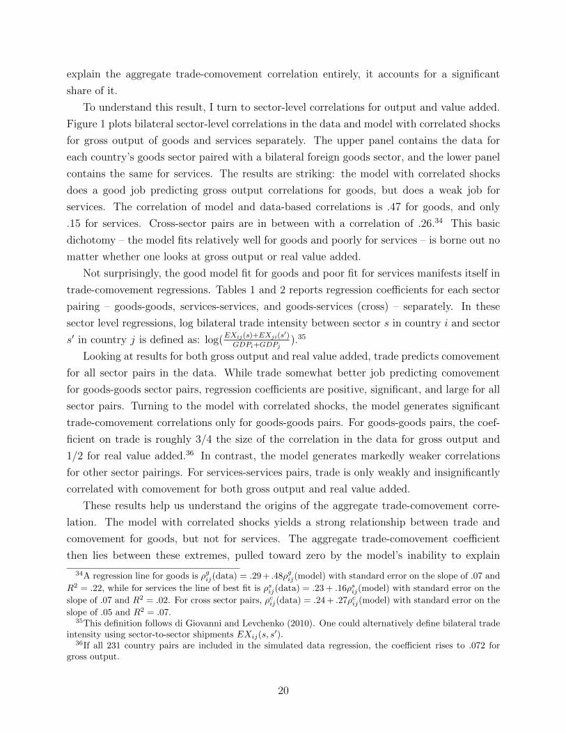
To understand this result, I turn to sector-level correlations for output and value added.

Figure 1 plots bilateral sector-level correlations in the data and model with correlated shocks

for gross output of goods and services separately. The upper panel contains the data for

each country’s goods sector paired with a bilateral foreign goods sector, and the lower panel

contains the same for services. The results are striking: the model with correlated shocks

does a good job predicting gross output correlations for goods, but does a weak job for

services. The correlation of model and data-based correlations is .47 for goods, and only

.15 for services. Cross-sector pairs are in between with a correlation of .26.34 This basic

dichotomy – the model fits relatively well for goods and poorly for services – is borne out no

matter whether one looks at gross output or real value added.

Not surprisingly, the good model fit for goods and poor fit for services manifests itself in

trade-comovement regressions. Tables 1 and 2 reports regression coefficients for each sector

pairing – goods-goods, services-services, and goods-services (cross) – separately. In these

sector level regressions, log bilateral trade intensity between sector s in country i and sector

s′ in country j is defined as: log(EXij(s)+EXji(s

′)

GDPi+GDPj).35

Looking at results for both gross output and real value added, trade predicts comovement

for all sector pairs in the data. While trade somewhat better job predicting comovement

for goods-goods sector pairs, regression coefficients are positive, significant, and large for all

sector pairs. Turning to the model with correlated shocks, the model generates significant

trade-comovement correlations only for goods-goods pairs. For goods-goods pairs, the coef-

ficient on trade is roughly 3/4 the size of the correlation in the data for gross output and

1/2 for real value added.36 In contrast, the model generates markedly weaker correlations

for other sector pairings. For services-services pairs, trade is only weakly and insignificantly

correlated with comovement for both gross output and real value added.

These results help us understand the origins of the aggregate trade-comovement corre-

lation. The model with correlated shocks yields a strong relationship between trade and

comovement for goods, but not for services. The aggregate trade-comovement coefficient

then lies between these extremes, pulled toward zero by the model’s inability to explain

34A regression line for goods is ρgij(data) = .29 + .48ρgij(model) with standard error on the slope of .07 and

R2 = .22, while for services the line of best fit is ρsij(data) = .23 + .16ρsij(model) with standard error on the

slope of .07 and R2 = .02. For cross sector pairs, ρcij(data) = .24 + .27ρcij(model) with standard error on the

slope of .05 and R2 = .07.35This definition follows di Giovanni and Levchenko (2010). One could alternatively define bilateral trade

intensity using sector-to-sector shipments EXij(s, s′).

36If all 231 country pairs are included in the simulated data regression, the coefficient rises to .072 forgross output.

20

services sector correlations. To raise the model implied trade-comovement correlation would

require introducing elements that raise the correlation of services sectors across countries.

Put differently, neither the measured correlation of services productivity shocks across coun-

tries, nor the transmission of idiosyncratic shocks through trade, is strong enough to generate

a large aggregate correlation of trade with aggregate output comovement in this model.

4.2 Propagation of Idiosyncratic Shocks via Trade

The model-based trade-comovement correlations reported above represent an upper bound

on the role of trade in generating comovement. Specifically, the trade-comovement regres-

sions confound two possible reasons why trade predicts comovement. Bilateral trade can

predict comovement either because it propagates shocks across border, or because it is a

proxy for another force that generates comovement. Of principal concern, countries that

trade more may have more correlated underlying productivity shocks.

To focus on pure propagation of idiosyncratic shocks, I turn to simulated data from the

model with uncorrelated shocks. Panel C of Tables 1 and 2 report trade-comovement regres-

sions for these simulations. In the first column, the aggregate trade-comovement correlation

declines substantially once one removes common shocks from the productivity process. This

decline is particularly pronounced for real value added in Table 2, where the coefficient is

roughly one-fifth the size of the coefficient in the model with correlated shocks and only

one-twentieth the size of the coefficient in the data.

The inability of the model here to generate a sizable correlation between trade and

comovement when shocks are uncorrelated is the analog to the Kose and Yi (2006) puzzle in

my framework. In a three-country IRBC model, Kose and Yi vary bilateral trade-intensity

exogenously by manipulating trade costs, holding the correlation of shocks across countries

constant. Then comparing value added correlations across equilibria with different trade

costs, they compute a trade-comovement quasi-regression coefficient that is at most 1/10th

the size of the coefficient in the data, a similar order of magnitude to the coefficients here.

Given that Kose-Yi examine a model without intermediate goods trade, this leads to the

conclusion that input trade does not “solve” the trade-comovement puzzle, at least in this

standard class of models. Despite the introduction of input trade into the IRBC model,

trade does not propagate shocks strongly enough to generate much comovement in aggregate

GDP. This implies that the positive coefficient on bilateral trade in data and the model with

correlated shocks arises because bilateral trade intensity proxies for the correlation of shocks

themselves.

An important caveat, however, is that there is significant propagation of idiosyncratic

21

shocks for gross output. The trade-comovement correlation in the model with uncorrelated

shocks is roughly 60% of the correlation in the model with correlated shocks. Thus, there

is an important discrepancy between the model’s ability to generate comovement in gross

output versus comovement in real value added. This result deserves separate attention, as

it highlights the role that intermediates play in this framework.

The discrepancy between the propagation mechanism for gross output versus real value

added is mostly clearly illustrated by examining cross-country correlations for goods pro-

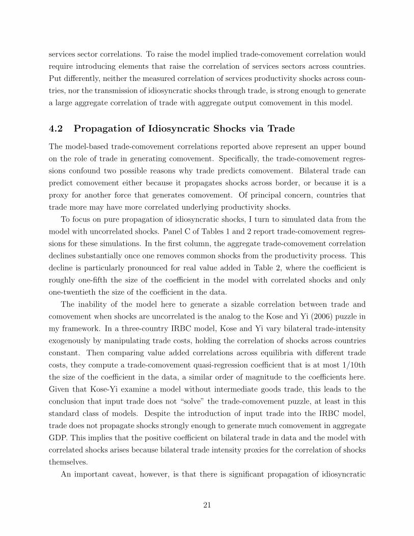
duction, so I focus on this sub-set of the data. For gross output of goods, propagation of

independent shocks explains roughly one-third of the observed comovement in the data. Fig-

ure 2 plots actual gross output correlations for goods against those predicted by the model

with uncorrelated shocks. There is a clear positive relationship, particularly among EU

country pairs. The U.S.-Canada outlier is particularly instructive. The predicted correlation

is roughly .23, while the actual correlation in the data is near .75, roughly a ratio of three

to one. More generally, this magnitude is consistent with the overall spread in the data. Fo-

cusing on EU-pairs, predicted correlations vary in the range (0, .15) while actual correlations

lie in the range (.25, .75), so the ratio of the ranges is roughly .5/.15 or three to one.37

These relationships are borne out in looking at the trade-comovement regressions for

goods trade in Panel C of Table 1, where the coefficient generated by the model with un-

correlated shocks is one-third the size of the coefficient in the model with correlated shocks

and one-quarter of that in the data. Thus, while two-thirds of the goods trade-comovement

relationship for gross output is due to correlated shocks in the model, one-third is explained

by the propagation of uncorrelated shocks across countries. At the same time, the model

generates much weaker comovement in real value added, even for goods-goods sector pairs.

One can see this by comparing the trade-comovement regression for goods in Panel C of

Table 2 to those in Table 1, where the coefficient for value added is near zero (just more

than 1/10 that for gross output).

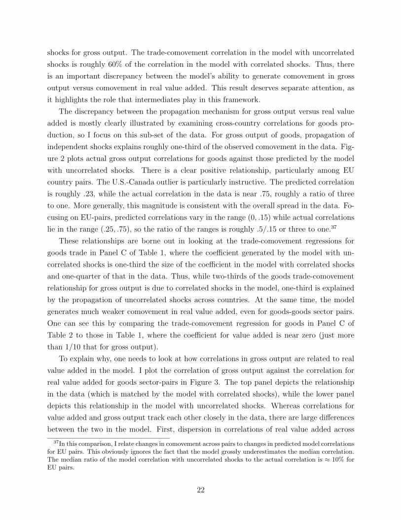
To explain why, one needs to look at how correlations in gross output are related to real

value added in the model. I plot the correlation of gross output against the correlation for

real value added for goods sector-pairs in Figure 3. The top panel depicts the relationship

in the data (which is matched by the model with correlated shocks), while the lower panel

depicts this relationship in the model with uncorrelated shocks. Whereas correlations for

value added and gross output track each other closely in the data, there are large differences

between the two in the model. First, dispersion in correlations of real value added across

37In this comparison, I relate changes in comovement across pairs to changes in predicted model correlationsfor EU pairs. This obviously ignores the fact that the model grossly underestimates the median correlation.The median ratio of the model correlation with uncorrelated shocks to the actual correlation is ≈ 10% forEU pairs.

22

country is much smaller than the variance of correlations in gross output. Second, the

correlation of gross output is typically larger (sometimes much larger) than the correlation

of real value added for individual country pairs.

These discrepancies shed light on the role of intermediate goods in the model. Recall

from the discussion in previous sections that gross output is a composite of real value added

and intermediate inputs, as in Equation (D3). The correlation of gross output can then be

decomposed into a weighted sum of the correlation of real value added across countries, the

correlation of input use across countries, and the cross-correlation of real value added and

input use:

ρij(Q) = wvvij ρij(V ) + wxxij ρij(X) + wvxij ρij(V,X) + wxvij ρij(V,X), (22)

where wvvij , wxxij , w

vxij , w

xvij are the appropriate weighting terms for each correlation, themselves

functions of the Cobb-Douglas share parameters and standard deviations of gross output, real

value added, and input use. To provide a visual sense of how these correlations aggregate, I

plot the correlations ρij(V ) and ρij(X) for select country pairs in Figure 4. As is evident, the

correlation in input use across countries dwarfs the correlation in real value added. Further,

the correlation of output lies somewhere in between, near the simple average of these two

correlations.38 Thus, the correlation of gross output is high because intermediate use is

highly correlated, not because value added is highly correlated.

The fact that intermediate use is highly correlated is direct evidence that productivity

shocks are being forcefully transmitted through cross-border production chains in the model.

Because the share of intermediates in gross output for goods is roughly 2/3, this translates

into significant output comovement. On the other hand, value added comovement is not high.

Recall that one reason value added comoves in the model is that factor supply responds to

relative prices. The low comovement of real value added indicates this channel is relatively

weak in the model. To raise comovement in value added, one would need to strengthen

this channel. In particular, the model would need to be adapted to translate the relatively

strong comovement in intermediate use into stronger comovement in value added. With this

motivation, I turn to analyzing whether input complementarity amplifies comovement.

38In the simulated data, the weights on each term are approximately equal (roughly 1/4) and the typicalcross-correlation (ρij(V,X) or ρij(V,X)) is relatively close to ρij(Q), lying between the extremes of ρij(V )and ρij(X). Hence, the simple average of ρij(V ) and ρij(X) approximates ρij(Q) quite well.

23

4.3 Complementarity and Comovement

A recent strain of thought holds that disruptions in input-sourcing produce large output

losses because inputs are complements in production. This argument surfaces in Burstein,

Kurz, and Tesar (2008), Jones (2011), Di Giovanni and Levchenko (2010), or news coverage of

the economic repercussions of the 2011 earthquake and tsunami in Japan for global supply

chains. This is intuitively plausible, as negative supply shocks in a particular country or

sector should be particular painful to upstream input users who have limited ability to

substitute toward using inputs from alternative suppliers, or toward using non-produced

factors of production (i.e., capital and labor) more intensively.

Building on these ideas, there are two distinct ways to introduce limited substitution for

intermediates into the production function used in previous sections. First, inputs may com-

plements to each other. In this instance, complementaries among inputs could be symmetric,

or complementaries could vary among subsets of inputs (e.g., home and foreign inputs could

be complements, while foreign inputs are substitutable among themselves). Second, inputs

may be complementary to other factors of production. Put differently, inputs may be com-

plementary to value added. To my knowledge, there is scant evidence as to which form of

complementarity is more important empirically, particularly, particularly in contexts with

imported intermediates. Therefore, I consider both types of complementarity in turn.

To generalize the set-up used above, I now assume that the production function is given

by:

Qit(s) = Zit(s) (θi(s)Vit(s)σ + (1− θi(s))Xit(s)

σ)1/σ

with Xit(s) =

(∑j

∑s′

ωxi (s′, s)Xjit(s′, s)η

)1/η

with Vit(s) = Kit(s)φLit(s)

1−φ,

(23)

where Vit(s) now denotes a Cobb-Douglas composite domestic factor, composed of capital and

labor, and φ denotes the capital share in this composite. The elasticity parameter σ controls

the substitution possibilities between intermediates and factor inputs, while η governs the

(symmetric) substitution among intermediates. Finally, θi(s) here is redefined as a share

parameter that can be chosen to match the intermediate input share in gross output, and

ωxi (s′, s) are share parameters that are calibrated to match bilateral intermediate goods flows.

There is scant evidence in the IRBC literature that guides calibration of complementarity

in the production function. Perhaps this is unsurprising, as nearly all IRBC models ignore

input trade and model production and consumption in value added terms. To illustrate the

24

consequences of complementarity, I simulate the model for two extreme cases. In the first

case, I assume the production function is Cobb-Douglas (setting σ effectively to zero) and

the intermediate goods aggregator is near-Leontief (setting η = −19, corresponding to an

elasticity of substitution equal to .05). In the second case, I assume the intermediate goods

aggregator is Cobb-Douglas (setting η effectively to zero) and the production function is

near-Leontief in Vit(s) and Xit(s) (setting σ = −19).39

Using this set-up, I re-simulate the model with uncorrelated productivity shocks as in

previous sections and run trade-comovement regressions in this new simulated data. I present

the results for sector-level correlations for the goods-goods sector pairing in Table 3. The

column labeled “benchmark” repeats results from previous tables for reference. The column

labeled “Complements w/in X” presents results for the simulation with σ = 0 and η = −19,

while the column labeled “Complements b/n V & X” presents results for the simulation with

σ = −19 and η = 0.

The results point to problems with the conventional view that complementarity is impor-

tant in explaining comovement. Introducing complementarity among intermediates (column

2) does substantially strengthen the propagation of shocks for gross output. In fact, the

model here generates a trade-comovement coefficient that exceeds the coefficient in data.

However, even with this extreme comovement in output, the model does not generate much

comovement in real value added. This implies that even extremely strong transmission of

shocks through input linkages fails to generate enough comovement in factor supplies across

countries to replicate real value added correlations.

In contrast, complementarity between inputs and factors fails on both counts: it nei-

ther generates comovement in gross output, nor real value added. In particular, the trade-

comovement correlation for gross output is even lower than in the benchmark model. What

is going on here? When agents are unable to substitute between factor inputs (V) and inter-

mediate inputs (X), the less responsive input effectively constrains fluctuations in demand

for the other input. In the model, factor input supply is fairly inelastic. This dampens

fluctuations in input use, which weakens the transmission of shocks through intermediate

linkages and lowers comovement in gross output.

These results seem to run counter to the received wisdom regarding the role of intermedi-

ates in propagation of shocks. In particular, they seem to contradict simulation evidence in

Burstein, Kurz, and Tesar (2008) that suggests complementary intermediates are important

for understanding the trade-comovement relationship. The results in this paper and their

39Strong complementary between factors and intermediates is common within the static computable gen-eral equilibrium trade literature, where Leontief production functions have been commonly employed. SeeKehoe and Kehoe (1994), for example.

25

work are, in fact, less contradictory than they first seem. The key difference is that Burstein

et al. specify complementarity in terms of value added, whereas I specify complementarity

in terms of gross output. In their model, the “production-sharing” (vertically integrated)

sector features a low elasticity of substitution between home and foreign value added. As

in the standard IRBC model, this low elasticity amplifies comovement, because low elas-

ticities imply volatile relative prices and strong transmission through the channel discussed

in Section 2.2. I do not directly assume home and foreign value added are complemen-

tary, but rather embed complementarity into the production function for gross output. One

way of reading my results is that complementarity of this form is not sufficient to induce

the complementarity between home and foreign value added needed to replicate observed

comovement.

4.4 Vertical Linkages in Trade-Comovement Regressions

In previous sections, I have used simple bivariate trade-comovement regressions to compare

model and data. Several recent papers have attempted to isolate the role of intermediates

in explaining comovement using more sophisticated specifications. Specifically, Di Giovanni

and Levchenko (2010) and Ng (2010) both construct proxies for bilateral vertical linkages

by combining trade and input-output data, and look at the partial effect of these linkages

controlling for overall bilateral trade intensity. Further, Di Giovanni and Levchenko also

estimate sector-level regressions with sector-pair and/or country-pair fixed effects to control

for common shocks across countries. It is an open question whether these augmented trade-

comovement regressions with vertical linkages can be interpreted as evidence of a causal

relationship between vertical linkages and output comovement. I therefore explore this ques-

tion using my simulated data.

Because Di Giovanni and Levchenko (2010) examine sector-level data, it is straightfor-

ward to map their empirical exercise to my framework and therefore I focus on their work. Di

Giovanni and Levchenko attack the identification problem by estimating trade-comovement

regressions at the sector level, pooling across sectors, and adding fixed effects to absorb par-

ticular unobservable shocks. Specifically, they construct a metric of bilateral vertical linkages

at the sector level to capture the intensity with which exports from sector s in country i

are used as intermediates by sector s′ in country j (and vice versa). This takes the form:[IO(s, s′)× Exportsij(s) + IO(s′, s)× Exportsji(s

′)], where IO(s, s′) is a measure of input-

output linkages between sectors s and s′ taken from a single country’s input-output table

and Exportsij(s) = log(

EXij(s)

GDPi+GDPj

)is the log of exports from i to j in sector s normalized

26

by the sum of value added in the source and destination countries.40

Then, Di Giovanni and Levchenko estimate the following regression:

ρij(s, s′) =α + βTradeij(s, s

′)

+ γ[IO(s, s′)× Exportsij(s) + IO(s′, s)× Exportsji(s

′)]

+ FE + εij(s, s′),

(24)

where Tradeij(s, s′) ≡ log

(EXij(s)+EXji(s

′)GDPi+GDPj

)and FE denotes fixed effects that vary by spec-

ification. One specification includes sector-pair fixed effects, while a second specification

includes sector-pair fixed effects and country-pair fixed effects. These fixed effects are intro-

duced to address concerns about omitted common shocks. The sector pair effects control

for worldwide sector-specific shocks (possibly correlated across sectors) that hit all countries

simultaneously. The country pair fixed effects control for aggregate shocks that may be

correlated across countries, but hit all sectors symmetrically within each country.41

I report the results of running these regressions in my data in Table 4. Focusing on results

for gross output, the regression results in the actual data are generally consistent with those

reported in Di-Giovanni and Levchenko. Both bilateral trade and vertical linkages (Trade×IO) are positively correlated with bilateral sector-level comovement. Vertical linkages are

significant in both specifications, while trade intensity is not significant when country fixed

are included (though the t-stat of 1.47 is sizable).42

Examining results in the model with correlated shocks, vertical linkages remain significant

and the coefficient magnitudes are the same or larger than those found in the data. Turning

to the model with uncorrelated shocks, however, the magnitude of the coefficient on vertical

linkages drops significantly, explaining at most 1/5 of the magnitude of the coefficients in

the data. Further, looking at real value added, the model with correlated shocks continues

to generate coefficients on vertical linkages similar to those in the data, though smaller in

magnitude. However, the sign on vertical linkages actually flips sign in regressions in the

simulated data with uncorrelated shocks.

Recall that the fixed effects are intended to control for correlated shocks driving corre-

lations in the data. If these fixed effects adequately control for these shocks, one should

expect that regression results in the model with uncorrelated shocks to be similar to those

40I use the direct input-requirements IO(s, s′) the U.S. to proxy for cross-sector input links. Di Giovanniand Levchenko also use input links for a single country.

41Ng (2010) embeds a vertical linkages metric into an aggregate trade-comovement regression, and thereforecannot use pair fixed effects to absorb common shocks. Instead, he includes other possible determinants ofcorrelations (e.g., financial openness, output composition, etc.) directly as control variables in the regression.

42One point to note is that my country sample is much smaller than Di Giovanni and Levchenko (2010),so lower significance levels may be expected.

27

in the data (alternatively, the model with correlated shocks). Given that they are not, this

suggests that vertical linkages proxies in the data may themselves be picking up shocks that

vary by country-pair and sector-pair that the fixed effects cannot absorb. As such, these

regressions are of dubious value as evidence that vertical linkages play an important role in

propagation of shocks.

5 Conclusion

This paper uses a multi-sector, many country extension of the IRBC model with trade

in both final and intermediate goods to dissect the trade-comovement puzzle. Using the

model, I attempt to refine our understanding of the trade comovement puzzle along several

dimensions.

First, input trade does not resolve the aggregate trade-comovement puzzle in a straight-

forward manner. That said, input trade does appear to play a role in explaining the relatively

good fit of the model for the gross output of goods. Surprisingly, however, transmission of

shocks through intermediate input channels does not generate strong comovement in value

added. Moreover, complementarity for intermediates within the production function does

not resolve this problem, or strengthen the trade transmission mechanism.

Second, and more generally, the aggregate trade-comovement correlation in the model

is induced by correlation of shocks across countries. In this, the low aggregate correlation

of trade with comovement in the model is due to the low correlation of shocks to services

productivity across countries. This suggests that closing the gap between model and data

will require expanding the set of shocks considered beyond productivity to include shocks

that synchronize services more forcefully.

Third, trade-comovement regressions are difficult to interpret because it is not generally

possible to control unobservable common shocks. This is true for plain-vanilla specifications,

as well as augmented specifications that include proxies for vertical linkages and/or employ

sector-level data with fixed effects. Model simulations with uncorrelated shocks suggest that

the “causal” role of bilateral trade and/or vertical linkages is much smaller than suggested

by raw regression estimates.

Despite these generally pessimistic results regarding the role of intermediates in gener-

ating comovement, there is promising evidence here that the introduction of intermediates

into macro models alters the role of trade as a conduit of shocks. While intermediates in this

benchmark IRBC framework do not replicate observed value added comovement, this may

speak to the shortcomings of the IRBC framework rather than to the role of inputs per se.

That is, there may be an important role for intermediates in models that capture the micro-

28

structure of trading relationships more accurately. For example, the bulk of intermediates

are traded within multinational firms, and this concentration of input trade among largest

firms in the economy may mean shocks to intermediate suppliers are passed to aggregates.

It is also true that many traded intermediates are tailored to a specific input purchaser –

e.g., screens for the iPad. This specificity at the firm-product level is difficult to capture in

the type of aggregate model developed in this paper. More careful consideration of these

microeconomic features of input trade would be useful in future work.

29

References

Ambler, S., E. Cardia, and C. Zimmerman (2002): “International transmission of thebusiness cycle in a multi-sector model,” European Economic Review, 46, 273–300.

Arkolakis, C., and A. Ramanarayanan (2009): “Vertical Specialization and Inter-national Business Cycle Synchronization,” Scandinavian Journal of Economics, 111(4),655–680.

Backus, D., P. Kehoe, and F. Kydland (1994): “Dynamics of the Trade Balance andthe Terms of Trade: The J-Curve?,” The American Economic Review, 84(1), 84–103.

Baxter, M. (1995): “International Trade and Business Cycles,” in Handbook of Interna-tional Economics, ed. by G. Grossman, and K. Rogoff, vol. 3, chap. 35, pp. 1801–1864.Elsevier.

Baxter, M., and M. Kouparitsas (2005): “Determinants of business cycle comovement:a robust analysis,” Journal of Monetary Economics, 52, 113–157.

Bems, R., R. Johnson, and K.-M. Yi (2010): “Demand Spillovers and the Collapse ofTrade in the Global Recession,” IMF Economic Review, 58(2), 295–326.

Bergin, P., R. Feenstra, and G. Hanson (2009): “Offshoring and Volatility: Evidencefrom Mexico’s Maquiladora Industry,” The American Economic Review, 99(4), 4.

Burstein, A., C. Kurz, and L. Tesar (2008): “Trade, production sharing, and theinternational transmission of business cycles,” Journal of Monetary Economics, 55, 775–795.

Calderon, C., A. Chong, and E. Stein (2007): “Trade intensity and business cyclesychronization: Are developing countries any different?,” Journal of International Eco-nomics, 71, 2–21.

Carvalho, V. M. (2008): “Aggregate Fluctuations and the Network Structure of Intersec-toral Trade,” Unpublished, CREi and Universitat Pompeu Fabra.

Chetty, R., A. Guren, D. Manoli, and A. Weber (2011): “Does Indivisible LaborExplain the Difference between Mico and Macro Elasticities? A Meta-Analysis of Exten-sive Margin Elasticities,” American Economic Review Papers and Proccedings, 101(2).

Cole, H., and M. Obstfeld (1991): “Commodity trade and international risk sharing,”Journal of Monetary Economics, 28, 3–24.

Conley, T., and B. Dupor (2003): “A Spatial Analysis of Sectoral Complementarity,”Journal of Political Economy, 111, 311–352.

Daudin, G., C. Rifflart, and D. Schweisguth (forthcoming): “Who Produces forWhom in the World Economy?,” Canadian Journal of Econoimcs.

30

di Giovanni, J., and A. Levchenko (2010): “Putting the Parts Together: Trade, Verti-cal Linkages and Business Cycle Comovement,” American Economic Journal: Macroeco-nomics, 2(2), 95–124.

Drozad, L., and J. Nosal (2008): “Long-Run Price Elasticity of Trade and the Trade-Comovement Puzzle,” Unpublished, University of Wisconsin.

Dupor, B. (1999): “Aggregation and irrelevance in multi-sector models,” Journal of Mon-etary Economics, 43, 391–409.

Engel, C., and J. Wang (2011): “International Trade in Durable Goods: UnderstandingVolatility, Cyclicality, and Elasticities,” Journal of International Economics, 83(1), 37–52.

Foerster, A., P.-D. Sarte, and M. Watson (2011): “Sectoral vs. Aggregate Shocks: AStructural Factor Analysis of Industrial Production,” The Journal of Political Economy,119(1), 1–38.

Frankel, J., and A. Rose (1998): “The Endogeneity of the Optimum Currency AreaCriteria,” The Economic Journal, 108, 1009–1025.

Heathcote, J., and F. Perri (2002): “Financial autarky and international businesscycles,” Journal of Monetary Economics, 49, 601–627.

Horvath, M. (1998): “Cyclicality and Sectoral Linkages: Aggregate Fluctuations fromIndependent Sectoral Shocks,” Review of Economic Dynamics, 1, 781–808.

(2000): “Sectoral shocks and aggregate fluctuations,” Journal of Monetary Eco-nomics, 45, 69–106.

Imbs, J. (2004): “Trade, Finance, Specialization, and Synchronization,” The Review ofEconomics and Statistics, 86, 723–734.

Inklaar, R., R. Jong-A-Pin, and J. de Haan (2008): “Trade and business cycle syn-chronization in OECD countries – A re-examination,” European Economic Review, 52(4),646–666.

Ishise, H. (2009): “Trade Costs and Business Cycle Transmission in a Multi-Country,Multi-Sector Model,” Unpublished Manuscript, Boston University.

(2010): “The World Has More Than Two Countries: Implications of Multi-CountryInternational Real Business Cycle Models,” Unpublished Manuscript, Boston University.

Johnson, R., and G. Noguera (2010): “Accounting for Intermediates: Production Shar-ing and Trade in Value Added,” Unpublished Manuscript, Dartmouth College.

Jones, C. (2011): “Intermediate Goods and Weak Links in the Theory of Economic Devel-opment,” American Economic Journal: Macroeconomics, 3(2), 1–28.

Juvenal, L., and P. S. Monteiro (2010): “Trade and Synchronization in a Multi-Country Economy,” Federal Reserve Bank of St. Louis Working Paper 2010-038C.

31

Kehoe, P., and T. Kehoe (1994): “A Primer on Static Applied General EquilibriumModels,” Federal Reserve Bank of Minneapolis Quarterly Review, 18(1), 2–16.

King, R., and S. Rebelo (1999): “Resuscitating Real Business Cycles,” in Handbook ofMacroeconomics, ed. by J. B. Taylor, and M. Woodford, vol. 1, chap. 14, pp. 927–1007.Elsevier.

Koopman, R., W. Powers, Z. Wang, and S.-J. Wei (2010): “Give Credit Where CreditIs Due: Tracing Value Added in Global Production Chains,” NBER Working Paper 16426.

Kose, M. A., and K. M. Yi (2006): “Can the standard international business cyclemodel explain the relation between trade and comovement?,” Journal of InternationalEconomics, 68, 267–295.

Long, J., and C. Plosser (1983): “Real Business Cycles,” Journal of Political Economy,91(1), 39–69.

Ng, E. C. (2010): “Production fragmentation and business-cycle comovement,” Journal ofInternational Economics, 82(1), 1–14.

O’Mahoney, M., and M. Timmer (2009): “Output, Input and Productivity Measures atthe Industry Level: The EU KLEMS Database,” The Economic Journal, 119, F374–F403.

Shea, J. (2002): “Complementarities and Comovements,” Journal of Money, Credit, andBanking, 34, 412–433.

Trefler, D., and S. C. Zhu (2010): “The Structure of Factor Content Predictions,”Journal of International Economics, 82, 195–207.

Uhlig, H. (1999): “A toolkit for analysing nonlinear dynamic stochastic models easily,”in Computational Methods for the Study of Dynamic Economies, ed. by R. Marimon, and

A. Scott, chap. 3, pp. 30–61. Oxford University Press.

Zimmerman, C. (1997): “International Real Business Cycles among Heterogeneous Coun-tries,” European Economic Review, 41, 319–355.

32

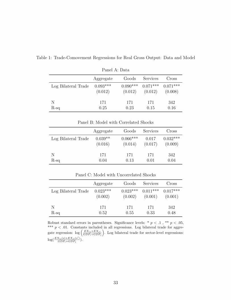
Table 1: Trade-Comovement Regressions for Real Gross Output: Data and Model

Panel A: Data

Aggregate Goods Services Cross

Log Bilateral Trade 0.093*** 0.090*** 0.071*** 0.071***(0.012) (0.012) (0.012) (0.008)

N 171 171 171 342R-sq 0.25 0.23 0.15 0.16

Panel B: Model with Correlated Shocks

Aggregate Goods Services Cross

Log Bilateral Trade 0.039** 0.066*** 0.017 0.032***(0.016) (0.014) (0.017) (0.009)

N 171 171 171 342R-sq 0.04 0.13 0.01 0.04

Panel C: Model with Uncorrelated Shocks

Aggregate Goods Services Cross

Log Bilateral Trade 0.023*** 0.023*** 0.011*** 0.017***(0.002) (0.002) (0.001) (0.001)

N 171 171 171 342R-sq 0.52 0.55 0.33 0.48

Robust standard errors in parentheses. Significance levels: * p < .1 , ** p < .05,*** p < .01. Constants included in all regressions. Log bilateral trade for aggre-

gate regression: log(

EXij+EXji

GDPi+GDPj

). Log bilateral trade for sector-level regressions:

log(EXij(s)+EXji(s

′)GDPi+GDPj

).

33

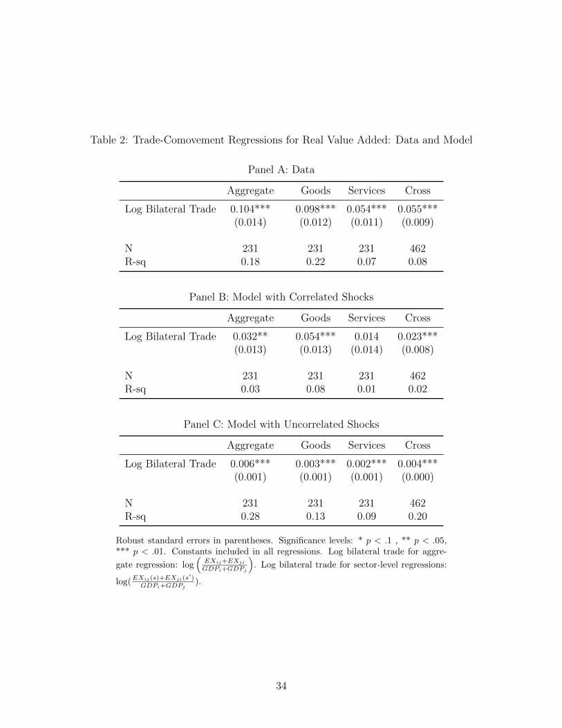
Table 2: Trade-Comovement Regressions for Real Value Added: Data and Model

Panel A: Data

Aggregate Goods Services Cross

Log Bilateral Trade 0.104*** 0.098*** 0.054*** 0.055***(0.014) (0.012) (0.011) (0.009)

N 231 231 231 462R-sq 0.18 0.22 0.07 0.08

Panel B: Model with Correlated Shocks

Aggregate Goods Services Cross

Log Bilateral Trade 0.032** 0.054*** 0.014 0.023***(0.013) (0.013) (0.014) (0.008)

N 231 231 231 462R-sq 0.03 0.08 0.01 0.02

Panel C: Model with Uncorrelated Shocks

Aggregate Goods Services Cross

Log Bilateral Trade 0.006*** 0.003*** 0.002*** 0.004***(0.001) (0.001) (0.001) (0.000)

N 231 231 231 462R-sq 0.28 0.13 0.09 0.20

Robust standard errors in parentheses. Significance levels: * p < .1 , ** p < .05,*** p < .01. Constants included in all regressions. Log bilateral trade for aggre-

gate regression: log(

EXij+EXji

GDPi+GDPj

). Log bilateral trade for sector-level regressions:

log(EXij(s)+EXji(s

′)GDPi+GDPj

).

34

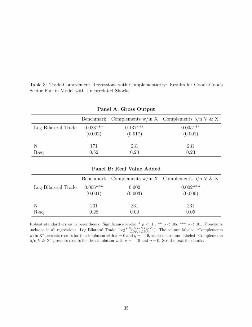
Table 3: Trade-Comovement Regressions with Complementarity: Results for Goods-GoodsSector Pair in Model with Uncorrelated Shocks

Panel A: Gross Output

Benchmark Complements w/in X Complements b/n V & X

Log Bilateral Trade 0.023*** 0.137*** 0.005***(0.002) (0.017) (0.001)

N 171 231 231R-sq 0.52 0.23 0.23

Panel B: Real Value Added

Benchmark Complements w/in X Complements b/n V & X

Log Bilateral Trade 0.006*** 0.002 0.002***(0.001) (0.003) (0.000)

N 231 231 231R-sq 0.28 0.00 0.05

Robust standard errors in parentheses. Significance levels: * p < .1 , ** p < .05, *** p < .01. Constants

included in all regressions. Log Bilateral Trade: log(EXij(s)+EXji(s

′)GDPi+GDPj

). The column labeled “Complements

w/in X” presents results for the simulation with σ = 0 and η = −19, while the column labeled “Complementsb/n V & X” presents results for the simulation with σ = −19 and η = 0. See the text for details.

35

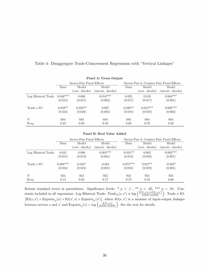
Table 4: Disaggregate Trade-Comovement Regressions with “Vertical Linkages”

Panel A: Gross Output

Sector-Pair Fixed Effects Sector-Pair & Country-Pair Fixed EffectsData Model Model Data Model Model

(corr. shocks) (uncorr. shocks) (corr. shocks) (uncorr. shocks)

Log Bilateral Trade 0.046*** 0.008 0.014*** 0.025 0.019 0.004***(0.013) (0.015) (0.002) (0.017) (0.017) (0.001)

Trade x IO 0.059** 0.058** 0.007 0.036** 0.054*** 0.008***(0.024) (0.028) (0.005) (0.018) (0.018) (0.002)

N 684 684 684 684 684 684R-sq 0.23 0.09 0.49 0.68 0.70 0.92

Panel B: Real Value Added

Sector-Pair Fixed Effects Sector-Pair & Country-Pair Fixed EffectsData Model Model Data Model Model

(corr. shocks) (uncorr. shocks) (corr. shocks) (uncorr. shocks)

Log Bilateral Trade 0.021 0.006 0.004*** -0.031** 0.002 0.002***(0.014) (0.013) (0.001) (0.013) (0.016) (0.001)

Trade x IO 0.088*** 0.044* -0.001 0.075*** 0.047** -0.002*(0.024) (0.024) (0.001) (0.016) (0.019) (0.001)

N 924 924 924 924 924 924R-sq 0.13 0.04 0.17 0.70 0.58 0.66

Robust standard errors in parentheses. Significance levels: * p < .1 , ** p < .05, *** p < .01. Con-

stants included in all regressions. Log Bilateral Trade: Tradeij(s, s′) ≡ log

(EXij(s)+EXji(s

′)GDPi+GDPj

). Trade x IO:[

IO(s, s′)× Exportsij(s) + IO(s′, s)× Exportsji(s′)], where IO(s, s′) is a measure of input-output linkages

between sectors s and s′ and Exportsij(s) = log(

EXij(s)GDPi+GDPj

). See the text for details.

36

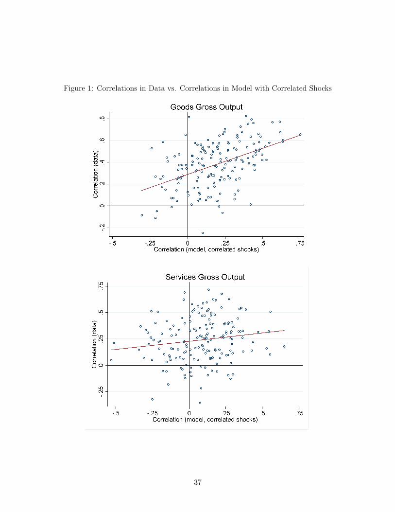
Figure 1: Correlations in Data vs. Correlations in Model with Correlated Shocks

37

Figure 2: Correlations in Data vs. Correlations in Model with Uncorrelated Shocks

38

Figure 3: Correlations in Gross Output vs. Correlations in Value Added: Model and Data

39

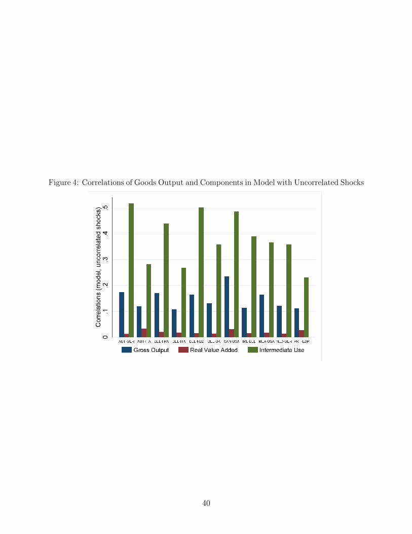
Figure 4: Correlations of Goods Output and Components in Model with Uncorrelated Shocks

40

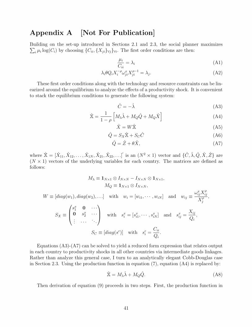
Appendix A [Not For Publication]

Building on the set-up introduced in Sections 2.1 and 2.3, the social planner maximizes∑i µi log(Ci) by choosing {Cii, {Xji}∀j}∀i. The first order conditions are then:

µiCii

= λi (A1)

λiθQiX−ρi ωxjiX

ρ−1ji = λj. (A2)

These first order conditions along with the technology and resource constraints can be lin-earized around the equilibrium to analyze the effects of a productivity shock. It is convenientto stack the equilibrium conditions to generate the following system:

C = −λ (A3)

X =1

1− ρ

[Mλλ+MQQ+MQX

](A4)

X = W X (A5)

Q = SXX + SCC (A6)

Q = Z + θX, (A7)

where X = [X11, X12, . . . , X1N , X21, X22, . . .]′

is an (N2 × 1) vector and {C, λ, Q, X, Z} are(N × 1) vectors of the underlying variables for each country. The matrices are defined asfollows:

Mλ ≡ 1N×1 ⊗ IN×N − IN×N ⊗ 1N×1,

MQ ≡ 1N×1 ⊗ IN×N ,

W ≡ [diag(w1), diag(w2), . . .] with wi = [wi1, · · · , wiN ] and wij ≡ωxijX

ρij

Xρj

,

SX ≡

sx1 0 · · ·0 sx2 · · ·... · · · . . .

with sxi = [sxi1, · · · , sxiN ] and sxij =Xij

Qi

,

SC ≡ [diag(sc)] with sci =CiiQi

.

Equations (A3)-(A7) can be solved to yield a reduced form expression that relates outputin each country to productivity shocks in all other countries via intermediate goods linkages.Rather than analyze this general case, I turn to an analytically elegant Cobb-Douglas casein Section 2.3. Using the production function in equation (7), equation (A4) is replaced by:

X = Mλλ+MQQ. (A8)

Then derivation of equation (9) proceeds in two steps. First, the production function in

41

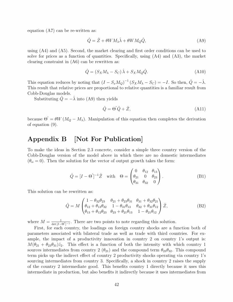
equation (A7) can be re-written as:

Q = Z + θWMλλ+ θWMQQ, (A9)

using (A4) and (A5). Second, the market clearing and first order conditions can be used tosolve for prices as a function of quantities. Specifically, using (A4) and (A3), the marketclearing constraint in (A6) can be rewritten as:

Q = (SXMλ − SC) λ+ SXMQQ. (A10)

This equation reduces by noting that (I − SxMQ)−1 (SXMλ − SC) = −I. So then, Q = −λ.This result that relative prices are proportional to relative quantities is a familiar result fromCobb-Douglas models.

Substituting Q = −λ into (A9) then yields

Q = Θ′Q+ Z, (A11)

because Θ′

= θW (MQ −Mλ). Manipulation of this equation then completes the derivationof equation (9).

Appendix B [Not For Publication]

To make the ideas in Section 2.3 concrete, consider a simple three country version of theCobb-Douglas version of the model above in which there are no domestic intermediates(θii = 0). Then the solution for the vector of output growth takes the form:

Q = [I −Θ′]−1Z with Θ =

0 θ12 θ13

θ21 0 θ23

θ31 θ32 0

. (B1)

This solution can be rewritten as:

Q = M

1− θ32θ23 θ21 + θ23θ31 θ31 + θ32θ21

θ12 + θ13θ32 1− θ31θ13 θ32 + θ31θ12

θ13 + θ12θ23 θ23 + θ21θ13 1− θ21θ12

Z, (B2)

where M = 1det [I−Θ′ ]−1 . There are two points to note regarding this solution.

First, for each country, the loadings on foreign country shocks are a function both ofparameters associated with bilateral trade as well as trade with third countries. For ex-ample, the impact of a productivity innovation in country 2 on country 1’s output is:M(θ21 + θ23θ31)z2. This effect is a function of both the intensity with which country 1sources intermediates from country 2 (θ21) and the compound term θ23θ32. This compoundterm picks up the indirect effect of country 2 productivity shocks operating via country 1’ssourcing intermediates from country 3. Specifically, a shock in country 2 raises the supplyof the country 2 intermediate good. This benefits country 1 directly because it uses thisintermediate in production, but also benefits it indirectly because it uses intermediates from

42

country 3 and country 3 intermediates are in turn produced using country 2 goods. Thus, thestructure of the entire production chain matters, not just bilateral input sourcing patterns.43

Second, there is multiplier effect that controls the magnitude of effect of shocks on eachcountry. To see this clearly, I re-write output growth for country 1 as:

Q1 = M1

[Z1 +

(θ21 + θ23θ31

1− θ32θ23

)Z2 +

(θ31 + θ32θ21

1− θ32θ23

)Z3

], (B3)

where I define M1 = 1−θ32θ23det [I−Θ′ ]−1 to be country 1’s multiplier. M1 summarizes how much

country 1 output increases with shocks to its own productivity and is generally greater thanone. Thus, the sensitivity of output to shocks for different countries can be decomposed intoa country specific effect Mi and a vector of weights on different shocks that varies acrosscountries.

Appendix C [Not For Publication]

The equilibrium conditions for the model in Section 3 are collected here. The first orderconditions for the consumer and production problems are given by:

∂Ui(Cit, Lit)

∂Cit= βEt

[∂Ui(Cit+1, Lit+1)

∂Cit+1

(rit+1

pfit+1

+ (1− δ)

)](C1)

∂Ui(Cit, Lit)

∂Lit=∂Ui(Cit, Lit)

∂Cit

wit

pfit(C2)

γi(s)pfitFit = pfit(s)Fit(s) (C3)

∂Fit(s)

∂Fjit(s)=pjt(s)

pfit(s)(C4)

αi(s)pit(s)Qit(s) = ritKit(s) (C5)

θi(s)pit(s)Qit(s) = pxit(s)Xit(s) (C6)

∂Xit(s)

∂Xjit(s′, s)=pjt(s

′)

pxit(s)(C7)

(1− αi(s)− θi(s))pit(s)Qit(s) = witLit(s). (C8)

43In a concrete example, the U.S. benefits from productivity increases in China not only because it importsfrom China, but also because the U.S. sources intermediates from Japan and Japan uses Chinese goods asinputs in production.

43

The market clearing conditions are given by:

Qit(s) =N∑j=1

S∑s′=1

Fijt(s) +Xijt(s, s′) (C9)

Fit = Cit +Kit+1 − (1− δ)Kit (C10)

pfitFit = witLit + ritKit + Ti (C11)

Kit =S∑s=1

Kit(s) (C12)

Lit =S∑s=1

Lit(s). (C13)

And remaining production functions and composite aggregators are given by:

Qit(s) = Zit(s)Kit(s)αi(s)Xit(s)

θi(s)Lit(s)1−αi(s)−θi(s) (C14)

Xit(s) = Xi(. . . , Xjit(s′, s), . . . ; s) (C15)

Fit(s) = Fi(. . . , Fjit(s), . . . ; s) (C16)

Fit =∏s

Fit(s)γi(s). (C17)

These equations represent 7N + 8(S × N) + 6N2 equations (minus one after choosinga numeraire) in the same number of unknowns. The unknowns include {Cit, Fit, Kit, Lit}for each country, {Qit(s), Kit(s), Xit(s), Lit(s), Fit(s), {Fjit(s)}j, {Xjit(s

′, s)}j,s′}i,s for each

country-sector, and prices {rit, wit, pfit, {pfit(s), p

xit(s), pit(s)}s}i.44 The {Ti} terms in the bud-

get constraint represent time-invariant transfers across countries, which allow me to fit themodel to a steady state with unbalanced trade. As discussed in the calibration section,I linearize around this unbalanced trade equilibrium assuming that trade imbalances areconstant.

With the functional forms for preferences and production functions given in Section3.4.1, these equilibrium can be linearized as follows. The linearized and stacked first order

44The equilibrium here can be easily reduced to the equilibrium defined in the main text via substitution.

44

conditions are given by:

0 = Et

[Ct − Ct+1 + β(1− δ)rt+1

](C18)

0 =1

εLt + Ct − wt + pft (C19)

0 = pft + Ft − pft (s)− Ft(s) (C20)

0 = Ft(s) +1

1− ρMipt(s)−

1

1− ρMj p

ft (s)−MjFt(s) (C21)

0 = pt(s) + Qt(s)− rt − Kt(s) (C22)

0 = pt(s) + Qt(s)− pxt (s)− Xt(s) (C23)

0 = X(s′, s)−Mj pt(s) +Mipt(s′)−MjQt(s) (C24)

0 = pt(s) + Qt(s)− wt − Lt(s), (C25)

where Mi ≡ IN×N ⊗ 1N×1 and Mj ≡ 1N×1 ⊗ IN×N . Here {rt, wt, pft , pft (s), p

xt (s), pt(s)} and

{Ct, Lt, Ft, Qt(s), Xt(s), Kt(s), Lt(s), Ft(s)} are vectors of prices and quantities, with elementi equal to the relevant variable for country i. The vector Ft(s) is a N2 dimensional vectorthat records final goods shipments for sector s, while Xt(s

′, s) is a N2 dimensional vectorthat records intermediates goods flows from sector s′ to sector s:

Ft(s) = [F11t(s), F12t(s), . . . , F1Nt(s), F21t(s), F22t(s), . . .]′

Xt(s′, s) = [X11t(s

′, s), X12t(s′, s), . . . , X1Nt(s

′, s), X21t(s′, s), X22t(s

′, s), . . .]′

The stacked and linearized market clearing conditions are given by:

0 = Qt(s)− SF (s)Ft(s)−∑s′

SX(s, s′)X(s, s′) (C26)

0 = Ft − diag(CiFi

)Ct − diag

(Ki

Fi

)Kt+1 + diag

(Ki(1− δ)

Fi

)Kt (C27)

0 = pft + Ft − diag

(wiLi

pfi Fi

)(wt + Lt)− diag

(riKi

pfi Fi

)(rt + Kt) (C28)

0 = Kt −S∑s=1

diag

(Ki(s)

Ki

)Kt(s) (C29)

0 = Lt −S∑s=1

diag

(Li(s)

Li

)Lt(s). (C30)

The bar notation denotes steady state values. The matrices SF (s) and SX(s, s′) collect the

45

share of output allocated to final and intermediate use in destinations as follows:

SF (s) ≡

sf1(s) 0 · · ·0 sf2(s) · · ·... · · · . . .

and SX(s, s′) ≡

sx1(s, s′) 0 · · ·0 sx2(s, s′) · · ·... · · · . . .

with sfi (s) = [sfi1(s), · · · , sfiN(s)], sfij(s) =

Fij(s)

Qi(s),

sxi (s, s′) = [sxi1(s, s′), · · · , sxiN(s, s′)], sxij(s, s

′) =Xij(s, s

′)

Qi(s).

Finally, the stacked and linearized production functions and aggregators are given by:

0=Qt(s)−Zt(s)−diag(αi(s))Kt(s)−diag(θi(s))Xt(s)−diag(1−αi(s)−θi(s))Lt(s) (C31)

0 = Xt(s)−∑s′

WX(s′, s)Xt(s′, s) (C32)

0 = Ft(s)−WF (s)Ft(s) (C33)

0 = Ft −∑s

diag(γi(s))Ft(s). (C34)

The matrices WF (s) and WX(s′, s) are sourcing shares for final and intermediate goods givenby:

WF (s) ≡ [diag(wf1 (s)), diag(wf2 (s)), . . .]

and WX(s′, s) ≡ [diag(wx1(s′, s)), diag(wx2(s′, s)), . . .]

with wfi (s) = [wfi1(s), · · · , wfiN(s)], wfij(s) ≡ωfij(s)Fij(s)

ρ

Fj(s)ρ,

and wxi (s′, s) = [θi1(s′, s), · · · , θiN(s′, s)].

To compute the dynamics, one needs to modify these conditions to reflect the choiceof numeraire. Further, to reduce the computational burden, I manually substitute out forfinal and intermediate goods shipments {{Fjit(s)}j, {Xjit(s

′, s)}j,s′}i,s}, thereby reducing thesize of the system by 6N2 (3174 with 23 countries) elements. Obviously other manualsubstitutions further reduce the dimensionality, but eliminating unknowns that increase inthe square of the number of countries is most important. I use Harald Uhlig’s “Toolkit forAnalyzing Nonlinear Dynamic Stochastic Models” in MATLAB to compute solutions to thissystem.45.

45See Uhlig (1999) or http://www2.wiwi.hu-berlin.de/institute/wpol/html/toolkit.htm

46

Appendix D [Not For Publication]

D.1 Final and Intermediate Goods Data and Calibration

The GTAP 7.1 Database is assembled by the Global Trade Analysis Project at Purdue Uni-versity based on three main sources: (1) World Bank and IMF macroeconomic and Balance ofPayments statistics; (2) United Nations Commodity Trade Statistics (Comtrade) Database;and (3) input-output tables from national statistical sources. To reconcile data from thesedifferent sources, GTAP researchers adjust the input-output tables to be consistent with in-ternational data sources. The data set includes internally consistent bilateral trade statisticscombined with domestic and import input-output tables for 94 countries plus 19 compositeregions covering 57 sectors in 2004.

From the GTAP database, I extract disaggregate input use tables for domestic inputpurchases and imported inputs. I then use bilateral trade data to split imported input useacross bilateral partners, assuming that input purchases from each source are proportionalto bilateral trade shares within a given sector. I split final goods imports across sourcecountries using trade shares in a similar way. This yields bilateral final and intermediategoods shipments for 57 sectors. I then aggregate data on sectoral production, trade, finaland intermediate shipments across sectors to form two composite sectors, defined as “goods”(including agriculture, natural resources, and manufacturing) and “services.”

This data is the main input to calibrating {θji(s′, s)} and {ωfji(s)}. According to theproducer’s first order condition (14), θji(s

′, s) is the ratio of expenditure on inputs fromcountry j to gross output:

θji(s′, s) =

pj(s′)Xji(s

′, s)

pi(s)Qi(s). (D1)

To calibrate {ωfji(s)}, note that the final goods producer’s first order condition (17) can berewritten in share form as:

pi(s)Fij(s)

pfjFj= γj(s)ω

fij(s)

(pi(s)

pfj (s)

)−ρ/(1−ρ)

, (D2)

wherepi(s)Fij(s)

pfj Fjis the share of final goods of sector s sourced from country i in total final

goods expenditure in j. The share of final expenditure on goods of sector s – γj(s) – canbe computed directly in the data. Then, choosing quantity units so that the price of grossoutput and the final goods are equal to one in the steady state, {ωfij} can computed bycombining these expenditure shares.

D.2 Productivity Adjustment

To understand the productivity adjustment, recall the discussion in Section 2.3.1 aboutdistinguishing gross output from real value added. At the sector level, gross output is a

47

composite of real value added and intermediate inputs:

Qit(s) = Vit(s)1−θi(s)Xit(s)

θi(s)

with Vit(s) ≡ Z1

1−θi(s)it Kit(s)

αi(s)

1−θi(s)Lit(s)1−αi(s)−θi(s)

1−θi(s)(D3)

Then, TFP measured using gross output is TFPQ

it(s) = Zit(s), while TFP measured us-

ing real value added is TFPV

it (s) = 11−θi(s)Zit(s). The two TFP measures are related by

TFPQ

it(s) = (1− θi(s))TFPV

it (s), so shocks to productivity measured using value added willbe larger than the corresponding shocks measured using gross output. This explains the needto adjust Σ and means that the correct covariance matrix for simulation is Σ = 1

T

∑tˆεtˆε′t,

where ˆεit(s) ≡ (1−θi(s))εit(s) as in the main text. The persistence parameter λi(s) obtainedin estimation of (21) can be directly used in simulations, as it does not depend on whichdefinition of productivity is used in the estimation.

48