
Trade Facilitation and the EU-ACP Economic Partnership ...
42
Trade Facilitation and the EU-ACP Economic Partnership Agreements: Who Has the Most to Gain? Maria Persson * April 24, 2007 Abstract The aim of the paper is to assess the potential benefits from trade facilitation in terms of increased trade flows both on average and specifically for the six regional groupings of ACP countries negotiating Economic Partnership Agreements (EPAs) with the EU. We use data from the World Bank’s Doing Business Database on the time required to export or import as indicators of cross-border transaction costs. A gravity model on two-way bilateral trade between 22 EU countries and 106 developing countries is estimated using a sample selection approach. We find that time delays both on the part of the exporter and the importer on average significantly decrease trade flows. We also find that this relationship is not linear: an extra day of waiting has smaller marginal effects if the time requirements are already high. On average, lowering border delays in the exporting country with one day from the sample mean would yield an export increasing effect of about 1 percent, while the same reduction in the importing country would give an import increase of about 0.5 percent. More specifically, we also find that countries negotiating in the EPA groups for SADC, West Africa, Eastern and Southern Africa (ESA), and the Caribbean have negative and significant effects from export transaction costs, as do EU and non-ACP developing countries. The effects for the SADC, West Africa and ESA groups are the largest. Countries in the Pacific, SADC, West Africa and the EU have significantly negative effects from import transaction costs, with the effects being largest for the two former groups. The results are generally robust to a number of alternative estimation methods such as Poisson estimation, IV estimation and the sample selection approach suggested by Helpman, Melitz and Rubinstein (2007). JEL classification: C21, F15, O24 Keywords: Trade Facilitation, EU, ACP, Economic Partnership Agreements, Gravity Model, Sample Selection * Lund University, Department of Economics, P.O. Box 7082, SE-220 07 Lund, Sweden; e-mail: [email protected] . The author thanks Yves Bourdet, Joakim Gullstrand, Karin Olofsdotter and Therese Nilsson for helpful comments.
Transcript of Trade Facilitation and the EU-ACP Economic Partnership ...
Trade Facilitation and the EU-ACP Economic
Partnership Agreements: Who Has the Most to Gain?
Maria Persson*
April 24, 2007
Abstract The aim of the paper is to assess the potential benefits from trade facilitation in terms of increased trade flows both on average and specifically for the six regional groupings of ACP countries negotiating Economic Partnership Agreements (EPAs) with the EU. We use data from the World Bank’s Doing Business Database on the time required to export or import as indicators of cross-border transaction costs. A gravity model on two-way bilateral trade between 22 EU countries and 106 developing countries is estimated using a sample selection approach. We find that time delays both on the part of the exporter and the importer on average significantly decrease trade flows. We also find that this relationship is not linear: an extra day of waiting has smaller marginal effects if the time requirements are already high. On average, lowering border delays in the exporting country with one day from the sample mean would yield an export increasing effect of about 1 percent, while the same reduction in the importing country would give an import increase of about 0.5 percent. More specifically, we also find that countries negotiating in the EPA groups for SADC, West Africa, Eastern and Southern Africa (ESA), and the Caribbean have negative and significant effects from export transaction costs, as do EU and non-ACP developing countries. The effects for the SADC, West Africa and ESA groups are the largest. Countries in the Pacific, SADC, West Africa and the EU have significantly negative effects from import transaction costs, with the effects being largest for the two former groups. The results are generally robust to a number of alternative estimation methods such as Poisson estimation, IV estimation and the sample selection approach suggested by Helpman, Melitz and Rubinstein (2007). JEL classification: C21, F15, O24 Keywords: Trade Facilitation, EU, ACP, Economic Partnership Agreements, Gravity Model, Sample Selection * Lund University, Department of Economics, P.O. Box 7082, SE-220 07 Lund, Sweden; e-mail: [email protected]. The author thanks Yves Bourdet, Joakim Gullstrand, Karin Olofsdotter and Therese Nilsson for helpful comments.
1 Introduction
The subject of trade facilitation, i.e. loosely speaking measures to lower transaction costs
related to cross-border trade procedures, has emerged as an important issue in the current
trade policy debate. This increased focus is no doubt related to the fact that many tariff
and non-tariff barriers have been reduced or eliminated in the past rounds of multilateral
trade negotiations, thus increasing the relative costs of inefficient trade procedures. It is
perhaps also an easier subject to tackle than some other imminent questions, considering
that no country gains in any obvious sense from having burdensome procedures. In the
words of European Union (EU) Trade Commissioner Peter Mandelson: “there are no
losers from trade facilitation reform, only winners”1.
In the World Trade Organization (WTO), trade facilitation is one of the four so-
called Singapore issues,2 all of which at one stage was supposed to be included in the
Doha Development Agenda, but where trade facilitation now is the only one remaining.3
Negotiations on trade facilitation in the Doha Round have been successful, but the
general breakdown of negotiations in the summer of 2006 made several countries
increase their attention to regional trade agreements and negotiations. In the context of
the EU’s trade relations with developing countries, much of the focus was transferred to
the ongoing negotiations about creating Economic Partnership Agreements (EPAs) with
six regional groups following the Cotonou Agreement’s pledge to replace the current
non-reciprocal and non-WTO compatible preferences for African, Caribbean and Pacific
(ACP) countries. Besides covering, among other things, issues of tariff and non-tariff
barriers to trade, these negotiations are supposed to address all Singapore issues.
In this paper, our goal is firstly to assess how large effects export and import
transaction costs related to cross-border trade procedures have on trade flows on average
and hence how big the potential benefits from trade facilitation are, and secondly, to
decompose these effects to see the specific potential for each EPA negotiating group as
1 See Nath and Mandelson (2006). Obviously, this is not strictly true, since some parties, such as customs officials, might lose from the inability to charge bribes, or from losing their jobs due to more efficient cross-border procedures. From a country welfare perspective though, one does indeed expect gains. 2 The others being trade and investment, competition policy and transparency in government procurements. 3 For an overview of the work going on in the WTO and in the negotiations, see WTO (2006).
well as for the EU.4 To this end, we use data from the World Bank’s (2007) Doing
Business Database on the time required to export or import in 2005 as indicators of trade
transaction costs. We estimate a gravity model on two-way bilateral trade between 22 EU
countries and 106 developing countries using a sample selection approach. In the model,
the average effects from export and import transaction costs are estimated separately, and
the relationship between transaction costs and trade flows is allowed to be non-linear
through the inclusion of quadratic transaction cost terms. By including several interaction
terms, we can also estimate the specific effect that trade transaction costs have on the EU
and each EPA group. Hence, we can get an estimate on how much trade would increase if
the transaction costs could be lowered, i.e. by successful trade facilitation reform, both on
average and specifically for EPA negotiating groups and the EU.
To the best of our knowledge, the potential effects of trade facilitation on EPA
groups have not been estimated before. Besides looking at a new question, on of the main
contributions of the paper compared with other papers in the general area of trade
facilitation, is that it uses a less restrictive model, allowing trade facilitation in both the
exporting and the importing country to affect bilateral trade flows, as well as allowing the
effect of trade facilitation to be non-linear. Further, it takes recent methodological
developments into account and, besides the main alternative of Heckman estimation,
estimates the model using a Poisson Pseudo-Maximum-Likelihood estimator,
instrumental variables estimation, and a new sample selection approach suggested by
Helpman, Melitz and Rubinstein (2007). The data on the time requirements for exports
have been used before, but not the data on border delays in the importing country.
To summarize our results, we find that time delays both on the part of the exporter
and the importer, proxying export and import transaction costs, on average significantly
decrease trade flows. We also find that this relationship is not linear: an extra day of
waiting has smaller marginal effects if the time requirements are already high. On
average, lowering border delays in the exporting country with one day (from the sample
4 Trade facilitation could affect a country’s economy through several links, such as trade flows, flows of foreign direct investment (FDI) or government revenue through the collection of trade taxes. In this paper, we only assess the effects on trade flows. For a discussion of these possible links, as well as an overview of studies, see Engman (2005).
3
mean) would yield an export increasing effect of about 1 percent, while the same
reduction in the importing country would give an import increase of about 0.5 percent.
Further, we find that countries negotiating in the EPA groups for the Southern
African Development Community (SADC), West Africa, Eastern and Southern Africa
(ESA), and the Caribbean have negative and significant effects from export transaction
costs, as do EU and non-ACP developing countries. Countries in the Pacific, SADC,
West Africa and the EU have significantly negative effects from import transaction costs.
Reducing border delays with one day from the within-group mean would increase exports
with between 1 and 8 percent, and the percentage effects of reducing import border
delays are generally of the same magnitude.
The next section will define trade facilitation more thoroughly and give an
overview of the framework for the EPA negotiations. Section three presents some
previous research. In section four, the methodology and data are discussed, where after
the estimation results are presented and interpreted. Section five summarizes and
concludes.
2 Background
2.1 Trade Facilitation Defined
Despite the recent years’ increased attention to trade facilitation, there is no real
consensus on how the term should be defined. Generally, there are at least two broad
ways of looking at the issue: either to use a narrow focus on what has been called “at the
border” procedures, or to use a wider perspective and also include so called “behind the
border” measures.
One common way to narrowly define trade facilitation originates with the WTO,
and is e.g. used by Engman (2005), stating that trade facilitation is “the simplification and
harmonization of international trade procedures”, where international trade procedures
are the “activities, practices and formalities involved in collecting, presenting,
communicating and processing data required for the movement of goods in international
trade”. This definition clearly limits the attention to what happens around the border.
4
With a slightly less narrow definition, the Doha Ministerial Declaration (WTO
2001) refers to trade facilitation as the “expediting [of] the movement, release and
clearance of goods, including goods in transit”. This leaves some room for looking at, for
instance, transport infrastructure.5
Defining trade facilitation even more broadly, Wilson, Mann and Otsuki (2003;
2005) include both direct border elements such as port efficiency and customs
administration, and some working more “inside the border”, such as domestic regulatory
environment and services infrastructure.
A nice summing up of the various ways to look at the matter is presented in Roy
and Bagai (2005). They say that “trade facilitation [...] aims to make trade procedures as
efficient as possible through the simplification and harmonization of documentation,
procedures and information flows.” They go on by saying that
In a narrow sense, it addresses the logistics of moving goods through ports or customs.
More broadly, it encompasses several inter-related factors such as customs and border
agencies, transport infrastructure (roads, ports, airports etc.), services and information
technology (as it relates to better logistics), regulatory environment, product standards,
Technical Barriers to Trade [...] etc. in order to lower [the] cost of moving goods between
destinations and across international borders.
In this study, we choose to work with the same kind of narrow perspective on trade
facilitation as Engman (2005). Borrowing a line from Roy and Bagai (2005), our
definition might be summarized as measures to decrease the transaction costs arising
from the “moving [of] goods through ports or customs”.6
2.2 Economic Partnership Agreements
In June 2000, relations between the EU and ACP countries began to change with the
signing of the Cotonou Agreement. This agreement, which entered into force in April 5 Note that the negotiations in the WTO are supposed to cover GATT article V (freedom of transit), article VIII (fees and formalities connected with importation and exportation) and article X (publication and administration of trade regulations); see WTO (2006). 6 Trade facilitation is clearly linked to the broader issue of Non-Tariff Barriers to Trade (NTBs), but the latter includes many more obstacles to trade. Even more generally, trade facilitation belongs to the literature on trade costs – for an overview see Anderson and van Wincoop (2004).
5
2003, stipulates that the non-reciprocal trade preferences previously applying to EU-ACP
trade only should remain in place until December 31, 2007, at the latest. At this date, new
WTO-compatible trade arrangements – Economic Partnership Agreements (EPAs) –
should enter into force.7
Negotiations between the EU and ACP countries have now been underway since
September 2002 to agree on the terms of the envisioned EPAs. The first phase of the
negotiations took place at an all-ACP-EU level and addressed general issues of interest to
all parties. A second phase of negotiations, launched 2003-2004, now takes place at a
regional level, where six groupings of ACP countries negotiate separately with the EU.
These regional negotiating groups are presented in table 1, with least developed countries
(LDCs) in italics. It is evident that not only are the EPA-negotiating groups quite
heterogeneous and contain both LDCs and non-LDCs, but there is also not necessarily
any straightforward connection between these EPA groups and existing regional
integration arrangements.8
Trade facilitation was not explicitly mentioned in the Cotonou Agreement, but in
an explanatory memorandum outlining the mandate authorizing the European
Commission to negotiate EPAs with ACP countries, it is stated that “EPAs should [...]
aim at simplifying the requirements and procedures related to imports and exports”
(European Commission 2002). In subsequent documents, it seems clear that the EU sees
all Singapore issues, including trade facilitation, as important parts of EPA agreements
(see European Commission 2007a). The ACP countries on their part mentioned trade
facilitation as one of several trade issues in the guidelines for negotiations (ACP Council
of Ministers 2002). Now, trade facilitation is explicitly an issue in all six EPA
negotiations. For an overview of trade facilitation in the EPA negotiations, see Nyamache
(2006).
7 Since the existing preferences do not apply to all developing countries, they are not covered by the Enabling Clause, and hence have to operate under a WTO-waiver. For the new preferences to be WTO-compatible, they would have to be reciprocal. For a description of ACP preferences since the 1960s and an estimation of their effects, see Persson and Wilhelmsson (forthcoming). 8 For a discussion of this and other EPA-related matters, see for instance Hinkle et al (2006).
6
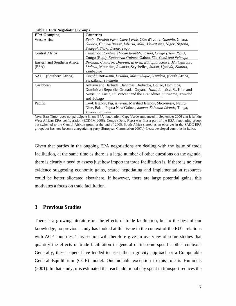
Table 1. EPA Negotiating Groups EPA Grouping Countries West Africa
Benin, Burkina Faso, Cape Verde, Côte d’Ivoire, Gambia, Ghana, Guinea, Guinea-Bissau, Liberia, Mali, Mauritania, Niger, Nigeria, Senegal, Sierra Leone, Togo
Central Africa
Cameroon, Central African Republic, Chad, Congo (Dem. Rep.), Congo (Rep.), Equatorial Guinea, Gabon, São Tomé and Principe
Eastern and Southern Africa (ESA)
Burundi, Comoros, Djibouti, Eritrea, Ethiopia, Kenya, Madagascar, Malawi, Mauritius, Rwanda, Seychelles, Sudan, Uganda, Zambia, Zimbabwe
SADC (Southern Africa)
Angola, Botswana, Lesotho, Mozambique, Namibia, (South Africa), Swaziland, Tanzania
Caribbean
Antigua and Barbuda, Bahamas, Barbados, Belize, Dominica, Dominican Republic, Grenada, Guyana, Haiti, Jamaica, St. Kitts and Nevis, St. Lucia, St. Vincent and the Grenadines, Suriname, Trinidad and Tobago
Pacific Cook Islands, Fiji, Kiribati, Marshall Islands, Micronesia, Nauru, Niue, Palau, Papua New Guinea, Samoa, Solomon Islands, Tonga, Tuvalu, Vanuatu
Note: East Timor does not participate in any EPA negotiation. Cape Verde announced in September 2006 that it left the West African EPA configuration (ECDPM 2006). Congo (Dem. Rep.) was first a part of the ESA negotiating group, but switched to the Central African group at the end of 2005. South Africa started as an observer in the SADC EPA group, but has now become a negotiating party (European Commission 2007b). Least developed countries in italics.
Given that parties in the ongoing EPA negotiations are dealing with the issue of trade
facilitation, at the same time as there is a large number of other questions on the agenda,
there is clearly a need to assess just how important trade facilitation is. If there is no clear
evidence suggesting economic gains, scarce negotiating and implementation resources
could be better allocated elsewhere. If however, there are large potential gains, this
motivates a focus on trade facilitation.
3 Previous Studies
There is a growing literature on the effects of trade facilitation, but to the best of our
knowledge, no previous study has looked at this issue in the context of the EU’s relations
with ACP countries. This section will therefore give an overview of some studies that
quantify the effects of trade facilitation in general or in some specific other contexts.
Generally, these papers have tended to use either a gravity approach or a Computable
General Equilibrium (CGE) model. One notable exception to this rule is Hummels
(2001). In that study, it is estimated that each additional day spent in transport reduces the
7
probability that the US will import from a particular country by 1 – 1.5 percent. Also,
each day that is saved in terms of shipping is estimated to represent 0.8 percent of the
value of manufactured goods.
3.1 Gravity Model Studies
Wilson, Mann and Otsuki (2005) use four separate indicators to measure trade
facilitation: port efficiency, customs environment, regulatory environment and service
sector infrastructure. The indicators are included in a gravity model for both the exporting
and importing country (except for the customs environment, which is only included for
the importing country). The underlying data, notably survey data from the Global
Competitiveness Report, is only available for rather few countries, leaving them with a
sample of 75 countries.9
The model is estimated with OLS with the dependent variable being manufactures
imports. All trade facilitation indicators are positive and significant in the regressions.
The authors further use these estimates to simulate what would happen if countries that
are below-average on a certain trade facilitation indicator would improve halfway to the
average for all countries. According to their findings, such a scenario would result in an
increase in trade of about 10 percent, out of which 0.8 percent would come from customs
environment improvements. Using a very similar design, Wilson, Mann and Otsuki
(2003) looks at the effect of trade facilitation on trade within the Asia Pacific Economic
Cooperation (APEC), with the main difference being that this paper only includes
measures of trade facilitation for the importer, and uses fixed effects for exporters. In the
authors’ preferred specification, all trade facilitation indicators are significant.
Djankov, Freund and Pham (2006) use the same data as this paper, i.e. World
Bank (2007), and estimate how time delays affect exports with the use of a gravity
9 Specifically, they have few developing countries, and especially only have data for Mauritius, Nigeria and South Africa for Sub-Saharan Africa. This is one major reason why we do not use the same data, since this would make it impossible to estimate effects on most EPA groups. Note that the variable customs environment, which is only included for the importing country, is the one that most closely resembles our indicators for potential trade facilitation.
8

model.10 Their preferred way of estimation is a difference gravity equation estimated on
similar exporters, i.e. exporters that are similar in location and factor endowments and
face the same trade barriers in foreign markets. Looking only at delays in the exporting
country, their main result is that, on average, for each additional day that a product is
delayed, trade is reduced by at least 1 percent. They also find that developing country
exports are significantly more affected by delays, and that exports of time-sensitive goods
are more influenced by exporters having to wait at the border.
Nordås, Pinali and Grosso (2006) estimate a gravity model with a Heckman
selection process to see both how time delays affect the size of observed trade flows, and
also the probability that trade between two countries will occur. The authors study
exports from 192 countries to Australia, Japan and the United Kingdom from 1996 to
2004. For all years but 2004, time for exports is proxied by a measure of the control of
corruption, while data for 2004 appears to come from the World Bank’s Doing Business
Report. Control of corruption is generally found to affect both the probability and volume
of exports positively, while the time for exports in most cases have a negative impact on
both the probability to export and the exported volumes.
Soloaga, Wilson and Mejía (2006) use the same methodology and type of data as
in Wilson, Mann and Otsuki (2005), but estimate the gravity model with a negative
binomial regression. Unlike in the latter study, they choose to include customs efficiency
also for the exporter. Most of the results are fairly similar to those obtained in Wilson,
Mann and Otsuki (2005), but puzzlingly, while they find the expected positive and
significant effect from customs efficiency in the exporting country, the corresponding
coefficient is robustly negative and significant for the importing country.
3.2 Studies Using CGE Models
OECD (2003) uses the GTAP model and database to explicitly assess benefits of trade
facilitation. Trade transaction costs are divided into direct and indirect costs, where the
former e.g. constitute costs for providing documentation, while the latter are costs
associated with delays at the border. Estimates of border waiting times for 80 countries 10 Note though that they use an earlier version of the data that has now been somewhat modified for a number of countries.
9
from the World Business Environment Survey are translated into direct costs using
Hummels’ (2001) estimate of the percentage trade value of saving a day of shipping time.
For measures of indirect costs, the authors use an index of border process quality
somewhat similar to the one used by Wilson, Mann and Otsuki (2005), and the country
with the highest quality indicator is then assumed to have direct costs of 1 percent of the
value of traded goods, while the country with the lowest quality indicator is assumed to
have costs of 15 percent.
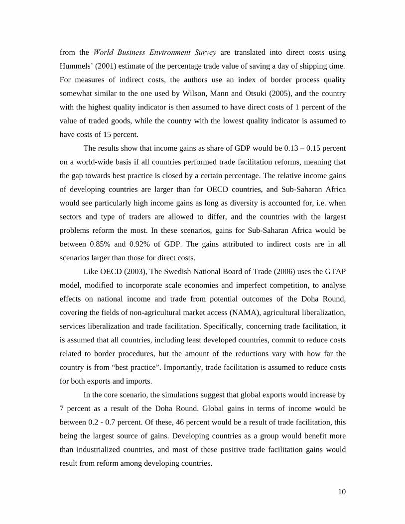
The results show that income gains as share of GDP would be 0.13 – 0.15 percent
on a world-wide basis if all countries performed trade facilitation reforms, meaning that
the gap towards best practice is closed by a certain percentage. The relative income gains
of developing countries are larger than for OECD countries, and Sub-Saharan Africa
would see particularly high income gains as long as diversity is accounted for, i.e. when
sectors and type of traders are allowed to differ, and the countries with the largest
problems reform the most. In these scenarios, gains for Sub-Saharan Africa would be
between 0.85% and 0.92% of GDP. The gains attributed to indirect costs are in all
scenarios larger than those for direct costs.
Like OECD (2003), The Swedish National Board of Trade (2006) uses the GTAP
model, modified to incorporate scale economies and imperfect competition, to analyse
effects on national income and trade from potential outcomes of the Doha Round,
covering the fields of non-agricultural market access (NAMA), agricultural liberalization,
services liberalization and trade facilitation. Specifically, concerning trade facilitation, it
is assumed that all countries, including least developed countries, commit to reduce costs
related to border procedures, but the amount of the reductions vary with how far the
country is from “best practice”. Importantly, trade facilitation is assumed to reduce costs
for both exports and imports.
In the core scenario, the simulations suggest that global exports would increase by
7 percent as a result of the Doha Round. Global gains in terms of income would be
between 0.2 - 0.7 percent. Of these, 46 percent would be a result of trade facilitation, this
being the largest source of gains. Developing countries as a group would benefit more
than industrialized countries, and most of these positive trade facilitation gains would
result from reform among developing countries.
10
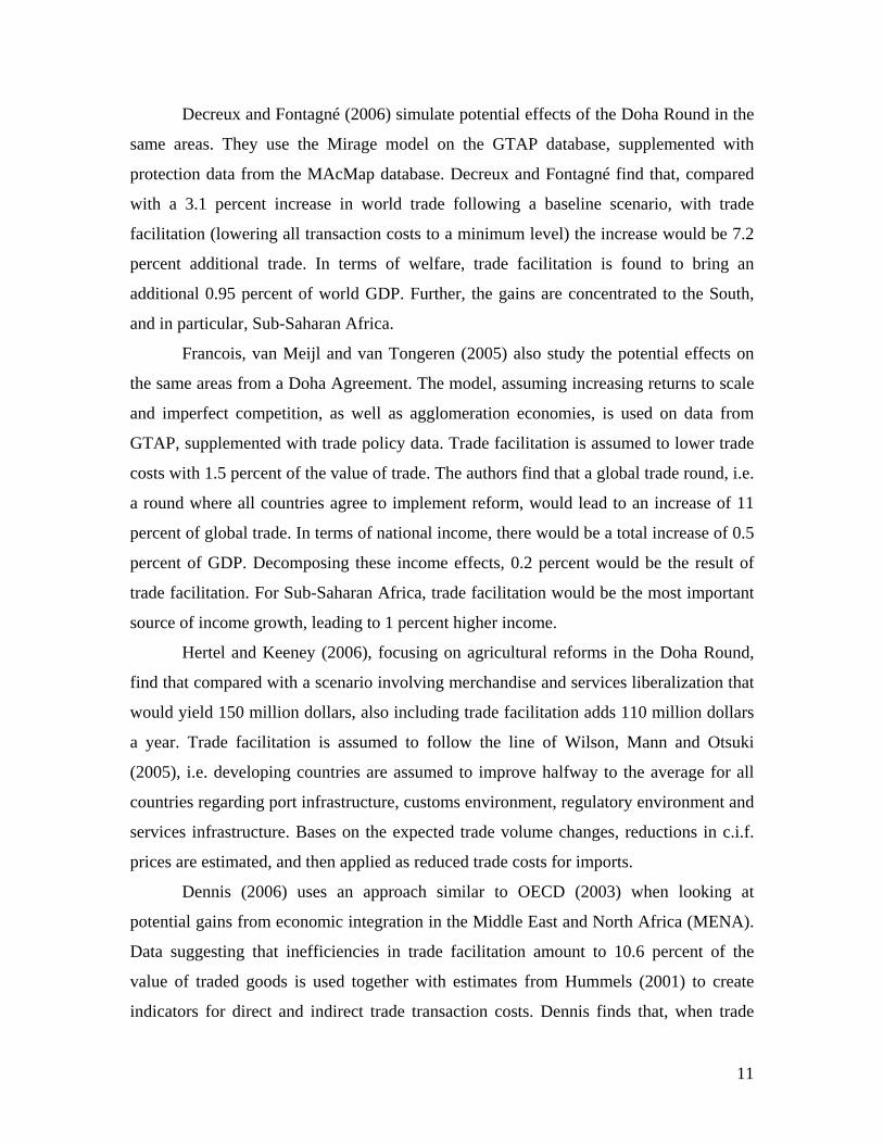
Decreux and Fontagné (2006) simulate potential effects of the Doha Round in the
same areas. They use the Mirage model on the GTAP database, supplemented with
protection data from the MAcMap database. Decreux and Fontagné find that, compared
with a 3.1 percent increase in world trade following a baseline scenario, with trade
facilitation (lowering all transaction costs to a minimum level) the increase would be 7.2
percent additional trade. In terms of welfare, trade facilitation is found to bring an
additional 0.95 percent of world GDP. Further, the gains are concentrated to the South,
and in particular, Sub-Saharan Africa.
Francois, van Meijl and van Tongeren (2005) also study the potential effects on
the same areas from a Doha Agreement. The model, assuming increasing returns to scale
and imperfect competition, as well as agglomeration economies, is used on data from
GTAP, supplemented with trade policy data. Trade facilitation is assumed to lower trade
costs with 1.5 percent of the value of trade. The authors find that a global trade round, i.e.
a round where all countries agree to implement reform, would lead to an increase of 11
percent of global trade. In terms of national income, there would be a total increase of 0.5
percent of GDP. Decomposing these income effects, 0.2 percent would be the result of
trade facilitation. For Sub-Saharan Africa, trade facilitation would be the most important
source of income growth, leading to 1 percent higher income.
Hertel and Keeney (2006), focusing on agricultural reforms in the Doha Round,
find that compared with a scenario involving merchandise and services liberalization that
would yield 150 million dollars, also including trade facilitation adds 110 million dollars
a year. Trade facilitation is assumed to follow the line of Wilson, Mann and Otsuki
(2005), i.e. developing countries are assumed to improve halfway to the average for all
countries regarding port infrastructure, customs environment, regulatory environment and
services infrastructure. Bases on the expected trade volume changes, reductions in c.i.f.
prices are estimated, and then applied as reduced trade costs for imports.
Dennis (2006) uses an approach similar to OECD (2003) when looking at
potential gains from economic integration in the Middle East and North Africa (MENA).
Data suggesting that inefficiencies in trade facilitation amount to 10.6 percent of the
value of traded goods is used together with estimates from Hummels (2001) to create
indicators for direct and indirect trade transaction costs. Dennis finds that, when trade
11

facilitation is added to regional liberalization initiatives within the MENA region, or with
the EU, the welfare gains become between 3 and 4 times higher.
4 Methodology
This section starts by discussing the model that we estimate to find potential effects of
trade facilitation on average and on each single EPA grouping. Then, we describe the
data used to measure the trade transaction costs that trade facilitation is meant to lower.
Lastly, the estimation results are presented and interpreted.
4.1 Model and Estimation Issues
To answer the question how cumbersome cross-border trade procedures affect trade
flows on average, and also specifically what the effects look like for the EPA groups and
the EU, we estimate a gravity equation including measures for export and import
transaction costs. The model is estimated on two-way trade flows between EU countries
and developing countries.
The gravity equation has been widely used to estimate the effects of e.g.
preferential trading arrangements and various trade costs,11 but has also at times been
criticized for lacking a solid theoretical basis. There is, however, a growing consensus
that this is not the case, and among the papers often cited are Anderson (1979),
Bergstrand (1985; 1989), Helpman and Krugman (1985) and Deardorff (1998). We
choose to use a model originating with Anderson and van Wincoop (2003). They derive
the gravity model using assumptions of constant elasticity of consumption (CES)
preferences and goods being differentiated by place of origin. In the model, Anderson
and van Wincoop assume unitary income elasticities, and include so called multilateral
resistance terms.12
11 For an overview of its application to preferential trade, see Greenaway and Milner (2002). 12 Capturing the fact that for any given level of bilateral barriers between countries i and j, if i has high barriers to its other trade partners, this will reduce the relative price of country j goods, and hence increase imports from j.
12
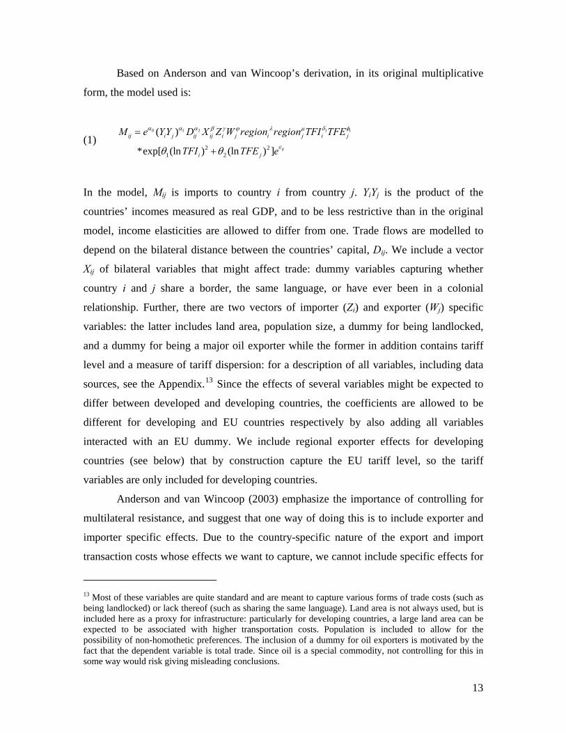
Based on Anderson and van Wincoop’s derivation, in its original multiplicative
form, the model used is:
(1) 0 1 2 1
2 21 2
( )
*exp[ (ln ) (ln ) ] ij
ij i j ij ij i j i j i j
i j
1M e YY D X Z W region region TFI TFE
TFI TFE e
α α α δβ γ ϕ λ μ
εθ θ
=
+
φ
In the model, Mij is imports to country i from country j. YiYj is the product of the
countries’ incomes measured as real GDP, and to be less restrictive than in the original
model, income elasticities are allowed to differ from one. Trade flows are modelled to
depend on the bilateral distance between the countries’ capital, Dij. We include a vector
Xij of bilateral variables that might affect trade: dummy variables capturing whether
country i and j share a border, the same language, or have ever been in a colonial
relationship. Further, there are two vectors of importer (Zi) and exporter (Wj) specific
variables: the latter includes land area, population size, a dummy for being landlocked,
and a dummy for being a major oil exporter while the former in addition contains tariff
level and a measure of tariff dispersion: for a description of all variables, including data
sources, see the Appendix.13 Since the effects of several variables might be expected to
differ between developed and developing countries, the coefficients are allowed to be
different for developing and EU countries respectively by also adding all variables
interacted with an EU dummy. We include regional exporter effects for developing
countries (see below) that by construction capture the EU tariff level, so the tariff
variables are only included for developing countries.
Anderson and van Wincoop (2003) emphasize the importance of controlling for
multilateral resistance, and suggest that one way of doing this is to include exporter and
importer specific effects. Due to the country-specific nature of the export and import
transaction costs whose effects we want to capture, we cannot include specific effects for
13 Most of these variables are quite standard and are meant to capture various forms of trade costs (such as being landlocked) or lack thereof (such as sharing the same language). Land area is not always used, but is included here as a proxy for infrastructure: particularly for developing countries, a large land area can be expected to be associated with higher transportation costs. Population is included to allow for the possibility of non-homothetic preferences. The inclusion of a dummy for oil exporters is motivated by the fact that the dependent variable is total trade. Since oil is a special commodity, not controlling for this in some way would risk giving misleading conclusions.
13
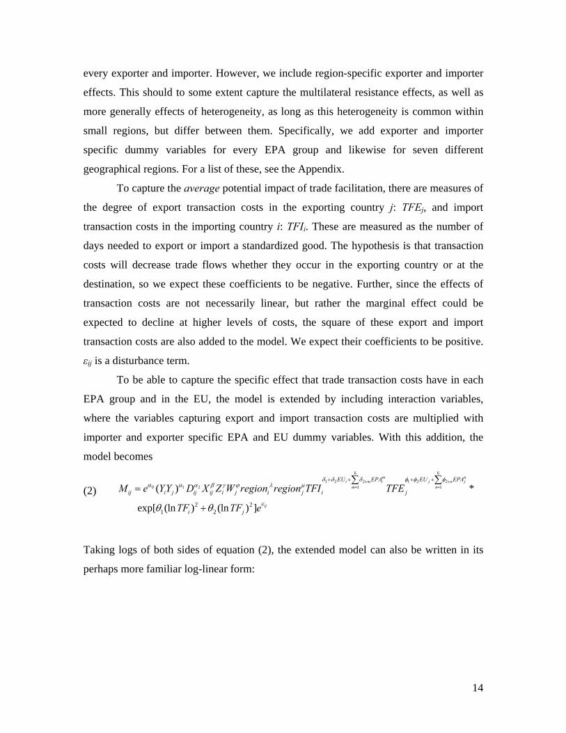
every exporter and importer. However, we include region-specific exporter and importer
effects. This should to some extent capture the multilateral resistance effects, as well as
more generally effects of heterogeneity, as long as this heterogeneity is common within
small regions, but differ between them. Specifically, we add exporter and importer
specific dummy variables for every EPA group and likewise for seven different
geographical regions. For a list of these, see the Appendix.
To capture the average potential impact of trade facilitation, there are measures of
the degree of export transaction costs in the exporting country j: TFEj, and import
transaction costs in the importing country i: TFIi. These are measured as the number of
days needed to export or import a standardized good. The hypothesis is that transaction
costs will decrease trade flows whether they occur in the exporting country or at the
destination, so we expect these coefficients to be negative. Further, since the effects of
transaction costs are not necessarily linear, but rather the marginal effect could be
expected to decline at higher levels of costs, the square of these export and import
transaction costs are also added to the model. We expect their coefficients to be positive.
εij is a disturbance term.
To be able to capture the specific effect that trade transaction costs have in each
EPA group and in the EU, the model is extended by including interaction variables,
where the variables capturing export and import transaction costs are multiplied with
importer and exporter specific EPA and EU dummy variables. With this addition, the
model becomes
(2)
6 6
1 2 2 1 2 20 1 11 2
2 21 2
( )
exp[ (ln ) (ln ) ]
m ni m i j n j
m n
ij
EU EPA EU EPA
ij i j ij ij i j i j i j
i j
M e YY D X Z W region region TFI TFE
TF TF e
δ δ δ φ φ φα α α β γ ϕ λ μ
εθ θ
+ += =
+ + + +∑ ∑=
+
*
Taking logs of both sides of equation (2), the extended model can also be written in its
perhaps more familiar log-linear form:
14
(3)
0 1 2
6
1 2 21
6
1 2 21
2 21 2
ln ln( ) ln
ln *ln *ln
ln *ln ln
(ln ) (ln )
ij i j ij ij i j i j
mi i i m i i
m
nj j j n j j
n
i j ij
M YY D X Z W region region
TFI EU TFI EPA TFI
TFE EU TFE EPA TFE
TFI TFE
α α α β γ ϕ λ μ
δ δ δ
φ φ φ
θ θ ε
+=
+=
= + + + + + + +
+ + +
+ + +
+ +
∑
∑
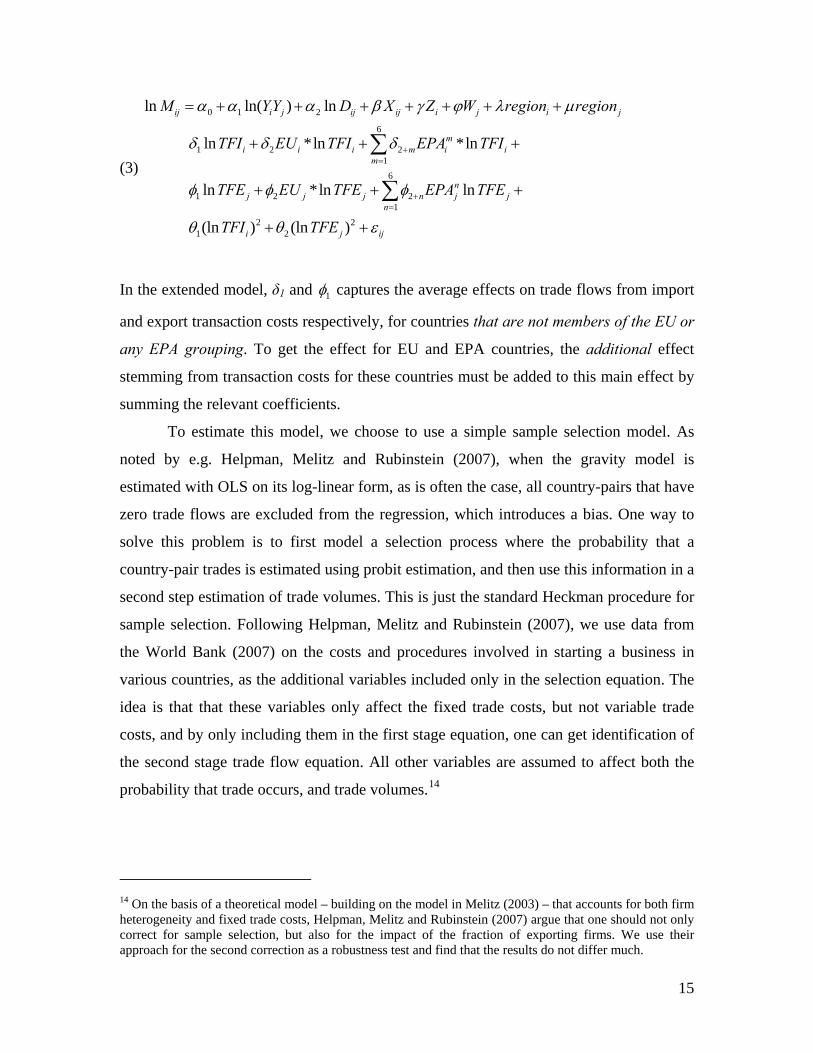
In the extended model, δ1 and 1φ captures the average effects on trade flows from import
and export transaction costs respectively, for countries that are not members of the EU or
any EPA grouping. To get the effect for EU and EPA countries, the additional effect
stemming from transaction costs for these countries must be added to this main effect by
summing the relevant coefficients.
To estimate this model, we choose to use a simple sample selection model. As
noted by e.g. Helpman, Melitz and Rubinstein (2007), when the gravity model is
estimated with OLS on its log-linear form, as is often the case, all country-pairs that have
zero trade flows are excluded from the regression, which introduces a bias. One way to
solve this problem is to first model a selection process where the probability that a
country-pair trades is estimated using probit estimation, and then use this information in a
second step estimation of trade volumes. This is just the standard Heckman procedure for
sample selection. Following Helpman, Melitz and Rubinstein (2007), we use data from
the World Bank (2007) on the costs and procedures involved in starting a business in
various countries, as the additional variables included only in the selection equation. The
idea is that that these variables only affect the fixed trade costs, but not variable trade
costs, and by only including them in the first stage equation, one can get identification of
the second stage trade flow equation. All other variables are assumed to affect both the
probability that trade occurs, and trade volumes.14
14 On the basis of a theoretical model – building on the model in Melitz (2003) – that accounts for both firm heterogeneity and fixed trade costs, Helpman, Melitz and Rubinstein (2007) argue that one should not only correct for sample selection, but also for the impact of the fraction of exporting firms. We use their approach for the second correction as a robustness test and find that the results do not differ much.
15
4.2 Data
The data used to measure the potential for trade facilitation comes from the World Bank
(2007) Doing Business Database. In the Trading Across Borders section of the database,
local trade professionals have answered a number of survey questions about, among other
things, how much time it would take to export or import a certain standardized good.15
Transaction costs at border crossings can arise due to a number of reasons, but
likely, the time required to export or import a good will be a good proxy for all these
transaction costs. For instance, having to collect many signatures or fill out many
documents might involve direct costs, but it will also increase the time needed to get the
good through customs. Port congestion and waiting due to insufficient staffing etc, will
also lead to higher time requirements. In turn, as noted by Djankov, Freund and Pham
(2006), long time delays will act as a tax on exports (or imports) due to at least three
factors: depreciation of the good, resources being allocated to storage and transport
instead of other uses, and the fact that long delays are associated with increased
uncertainty about delivery times. Therefore, we argue that border delays are not only a
good indicator for the customs environment, but more specifically, a good proxy for the
transaction costs that trade facilitation is meant to lower.16
The data on the number of days needed to export or import the standardized good
is available for 155 countries for 2005. Part of the data has been used to measure trade
facilitation in Djankov, Freund and Pham (2006). However, unlike that paper, we use the
data over time needed for both exports and imports, corresponding to the hypothesis that
15 To make the data comparable across countries, it is assumed that the hypothetical trading firm is a private and fully domestically owned business with a minimum of 200 employees that is located in the country’s most populous city and exports more than 10 percent of its sales to international markets. The good is assumed to be non-hazardous and not include any military arms or equipment, not to require refrigeration or any special environment, not to require any special phytosanitary or environmental safety standards, and to be shipped in a dry-cargo, 20-foot, full container load. Trade is assumed to take place by ocean transportation through the closest or main port from the most populous city (the port may be located in another city or country). For more specifics, see World Bank (2007), or Djankov, Freund and Pham (2006) that offers an excellent review of the data. 16 As we are working with a relatively narrow definition of trade facilitation, concentrating on what happens at the border, there might be some concern that the time measure picks up too many aspects, i.e. also obstacles behind the border. This should not be a major problem however, since about 75 percent of the delays in the sample are due to “administrative hurdles” – customs procedures, tax procedures, clearances and cargo inspections (Djankov, Freund and Pham, 2006).
16
not only what a country does on its own matters, but the situation in its trading partners
will also affect bilateral trade flows.
There are some possible concerns with using this data as an indicator of potential
trade facilitation. OECD (2003) note that the indirect costs that arise due to waiting at the
border might differ, not only between countries, which we do measure with our data, but
also within countries due to the sensitivity of the good and the size of the firm. If this is
the case, the measure of trade facilitation we use is not ideal, since this by design only
captures the time it takes a large firm to export or import a relatively time-insensitive
good. A further problem with the data, related to this, is that for every country, we only
know the average time needed to export or import to all countries. If the composition of
trade varies with trading partners, this is not a very good measure for the transaction costs
in a specific bilateral trade flow. We try to explore the consequences of this in the
robustness section below, but we would argue that the specific sample that we use
reduces the problem. We include bilateral trade flows between EU countries and
developing countries, where the composition of trade can be expected to be more even
than if we had also included trade between developing countries, or between
industrialized countries. Further, there is likely a high correlation between the time
requirements for different kinds of goods, so if border delays for the survey’s
standardized good are large, this should be a good indicator of a generally inefficient
customs environment.
Using the Doing Business Database to measure the potential for trade facilitation
gives us a sample of 22 EU countries: Cyprus, Luxembourg and Malta disappear. To get
a well-defined sample of developing countries, all countries that were eligible for
preferences under the Generalized System of Preferences (GSP) are included. As is the
case with the EU, some countries disappear due to missing data. The sample of
developing countries can be seen in the Appendix, together with a description of the other
data used, including sources.
Descriptive Statistics
It is interesting to look at some descriptive statistics for the measures of potential trade
facilitation. Starting with the time that is required to export a good, as is evident from
17
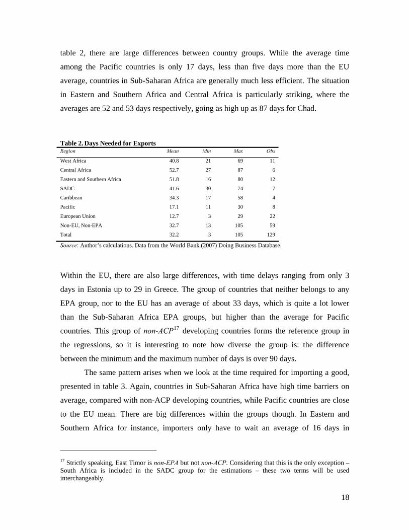
table 2, there are large differences between country groups. While the average time
among the Pacific countries is only 17 days, less than five days more than the EU
average, countries in Sub-Saharan Africa are generally much less efficient. The situation
in Eastern and Southern Africa and Central Africa is particularly striking, where the
averages are 52 and 53 days respectively, going as high up as 87 days for Chad.
Table 2. Days Needed for Exports Region Mean Min Max Obs
West Africa 40.8 21 69 11
Central Africa 52.7 27 87 6
Eastern and Southern Africa 51.8 16 80 12
SADC 41.6 30 74 7
Caribbean 34.3 17 58 4
Pacific 17.1 11 30 8
European Union 12.7 3 29 22
Non-EU, Non-EPA 32.7 13 105 59
Total 32.2 3 105 129
Source: Author’s calculations. Data from the World Bank (2007) Doing Business Database.
Within the EU, there are also large differences, with time delays ranging from only 3
days in Estonia up to 29 in Greece. The group of countries that neither belongs to any
EPA group, nor to the EU has an average of about 33 days, which is quite a lot lower
than the Sub-Saharan Africa EPA groups, but higher than the average for Pacific
countries. This group of non-ACP17 developing countries forms the reference group in
the regressions, so it is interesting to note how diverse the group is: the difference
between the minimum and the maximum number of days is over 90 days.
The same pattern arises when we look at the time required for importing a good,
presented in table 3. Again, countries in Sub-Saharan Africa have high time barriers on
average, compared with non-ACP developing countries, while Pacific countries are close
to the EU mean. There are big differences within the groups though. In Eastern and
Southern Africa for instance, importers only have to wait an average of 16 days in
17 Strictly speaking, East Timor is non-EPA but not non-ACP. Considering that this is the only exception – South Africa is included in the SADC group for the estimations – these two terms will be used interchangeably.
18
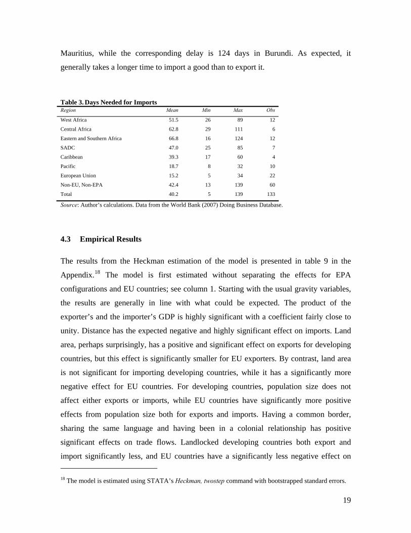
Mauritius, while the corresponding delay is 124 days in Burundi. As expected, it
generally takes a longer time to import a good than to export it.
Table 3. Days Needed for Imports Region Mean Min Max Obs
West Africa 51.5 26 89 12
Central Africa 62.8 29 111 6
Eastern and Southern Africa 66.8 16 124 12
SADC 47.0 25 85 7
Caribbean 39.3 17 60 4
Pacific 18.7 8 32 10
European Union 15.2 5 34 22
Non-EU, Non-EPA 42.4 13 139 60
Total 40.2 5 139 133
Source: Author’s calculations. Data from the World Bank (2007) Doing Business Database.
4.3 Empirical Results
The results from the Heckman estimation of the model is presented in table 9 in the
Appendix.18 The model is first estimated without separating the effects for EPA
configurations and EU countries; see column 1. Starting with the usual gravity variables,
the results are generally in line with what could be expected. The product of the
exporter’s and the importer’s GDP is highly significant with a coefficient fairly close to
unity. Distance has the expected negative and highly significant effect on imports. Land
area, perhaps surprisingly, has a positive and significant effect on exports for developing
countries, but this effect is significantly smaller for EU exporters. By contrast, land area
is not significant for importing developing countries, while it has a significantly more
negative effect for EU countries. For developing countries, population size does not
affect either exports or imports, while EU countries have significantly more positive
effects from population size both for exports and imports. Having a common border,
sharing the same language and having been in a colonial relationship has positive
significant effects on trade flows. Landlocked developing countries both export and
import significantly less, and EU countries have a significantly less negative effect on 18 The model is estimated using STATA’s Heckman, twostep command with bootstrapped standard errors.
19
exports from being landlocked. LDCs both export and import significantly less, as do
major oil exporters. The average tariff in developing countries has a significant negative
impact on imports, and there is also a significant negative effect from the tariff dispersion
variable: if high tariffs are concentrated on certain sectors, interpreted as tariff peaks, this
is negative for trade flows.
Looking at the variables of real interest, both the average level of export
transaction costs and import transaction costs have the expected negative coefficients,
and both are highly significant. The magnitude of the coefficient for export transaction
costs is somewhat larger at -1.5, with the corresponding coefficient for import transaction
costs being about -1.3. These coefficients are of the same magnitude as the coefficient for
distance. Interestingly, the squared trade facilitation variables are also significant and
have the expected positive sign. A reasonable interpretation must therefore be that border
delays, proxying indirect trade transaction costs, on average have a significant negative
effect on trade flows both when they occur in the exporting country, and at the
destination. The marginal effect of an extra day of waiting is however not constant: when
the level of transaction costs is already high, waiting a little longer will be less harmful
than it would have been at lower levels.19
Turning now to the baseline model estimated with interaction effects for EPA
groups and the EU, the results can be seen in column two of table 9. For most variables,
the results are very similar to the model without interaction effects. The results for the
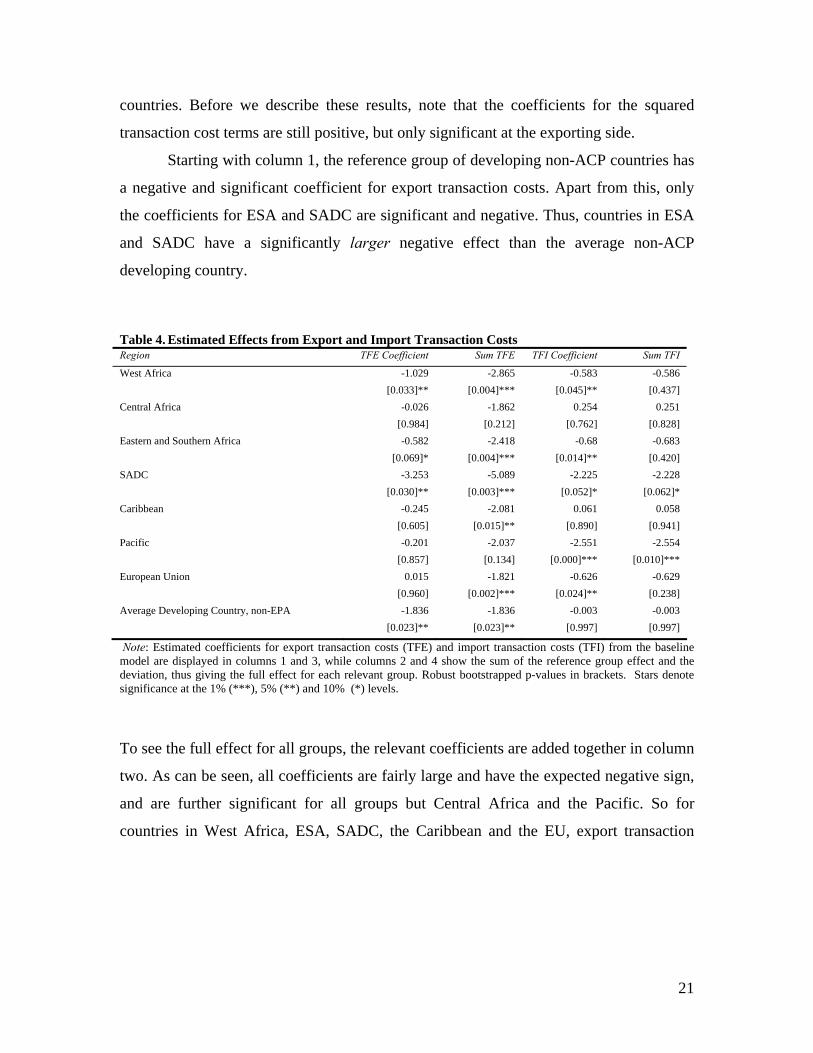
trade facilitation variables are reproduced in table 4. It is important to note the different
interpretation: Before the inclusion of interaction effects for EPA and EU countries, the
main transaction cost variables for exports, TFE, and imports, TFI, measured the average
effect of transaction costs for all countries. Now, they measure the average effect for the
reference group not included in any interaction terms, i.e. developing, non-ACP
19 Since we use a Heckman procedure, the first stage probit estimation gives us some extra results concerning the impact of various variables on the likelihood that positive trade flows occur between two countries. This paper focuses on the effect on trade volumes from trade transaction costs, so we will not have much to say about this issue, but the results are displayed in table 9. For most variables, the effect on the likelihood of trade and on trade volumes goes in the same direction, but there are some exceptions, such as the fact that being a major oil exporter has a negative effect on import volumes, but increases the likelihood that imports at all will take place. Further, in some specifications, we get different signs for the import transaction costs variables in the first and second stage estimations. We do not have a good explanation for this.
20
countries. Before we describe these results, note that the coefficients for the squared
transaction cost terms are still positive, but only significant at the exporting side.
Starting with column 1, the reference group of developing non-ACP countries has
a negative and significant coefficient for export transaction costs. Apart from this, only
the coefficients for ESA and SADC are significant and negative. Thus, countries in ESA
and SADC have a significantly larger negative effect than the average non-ACP
developing country.
Table 4. Estimated Effects from Export and Import Transaction Costs Region TFE Coefficient Sum TFE TFI Coefficient Sum TFI
West Africa -1.029 -2.865 -0.583 -0.586 [0.033]** [0.004]*** [0.045]** [0.437] Central Africa -0.026 -1.862 0.254 0.251 [0.984] [0.212] [0.762] [0.828] Eastern and Southern Africa -0.582 -2.418 -0.68 -0.683 [0.069]* [0.004]*** [0.014]** [0.420] SADC -3.253 -5.089 -2.225 -2.228 [0.030]** [0.003]*** [0.052]* [0.062]* Caribbean -0.245 -2.081 0.061 0.058 [0.605] [0.015]** [0.890] [0.941] Pacific -0.201 -2.037 -2.551 -2.554 [0.857] [0.134] [0.000]*** [0.010]*** European Union 0.015 -1.821 -0.626 -0.629 [0.960] [0.002]*** [0.024]** [0.238] Average Developing Country, non-EPA -1.836 -1.836 -0.003 -0.003 [0.023]** [0.023]** [0.997] [0.997]
Note: Estimated coefficients for export transaction costs (TFE) and import transaction costs (TFI) from the baseline model are displayed in columns 1 and 3, while columns 2 and 4 show the sum of the reference group effect and the deviation, thus giving the full effect for each relevant group. Robust bootstrapped p-values in brackets. Stars denote significance at the 1% (***), 5% (**) and 10% (*) levels.
To see the full effect for all groups, the relevant coefficients are added together in column
two. As can be seen, all coefficients are fairly large and have the expected negative sign,
and are further significant for all groups but Central Africa and the Pacific. So for
countries in West Africa, ESA, SADC, the Caribbean and the EU, export transaction
21
costs have significantly negative effects on export flows. The largest negative effects are
found for SADC.20
Looking now at the corresponding coefficients for import transaction costs, a first
thing to notice in column three is that the reference group coefficient is not significantly
different from zero. Hence, we cannot find any negative effects from import transaction
costs for the average non-ACP developing country. This means that the other coefficients
in column three really could be interpreted as the full import transaction cost effects,
since they capture the deviation from the reference group, i.e. the deviation from zero.
Noting that the coefficients for Western Africa, ESA, SADC, the Pacific and the EU all
are negative and significant, one can therefore interpret this as saying that these groups,
unlike the average non-ACP developing countries, experience a significantly negative
effect from import transaction costs. For completeness, the relevant coefficients are also
added together in column four, but we would argue that column three is the relevant one
to study. One interesting thing to notice is that, for almost all cases, the coefficients for
export transaction costs are larger than for import transaction costs, suggesting that
border delays at the origin would be more of a problem than inefficient border procedures
at the destination. The only exception to this rule is the group of Pacific countries, where
we cannot find any evidence of significant effects from export transaction costs, while
they have a large, significantly negative effect from import transaction costs.
Having found evidence suggesting that delays at the border by giving rise to
transaction costs can influence trade flows, a natural policy question is how much that
can be gained by reducing these border delays. Using coefficients from the baseline
regression without interaction effects, we find that for the whole sample, lowering border
delays from the mean with one day would yield an export increasing effect of about 1
20 It is important to note that because of the quadratic term included in the model, these coefficients are not actual elasticities. The expression for the elasticities will also include the level of transaction costs, so that higher levels of costs are associated with smaller elasticities.
22
percent. The corresponding import trade facilitation would result in an increase of about
0.5 percent.21
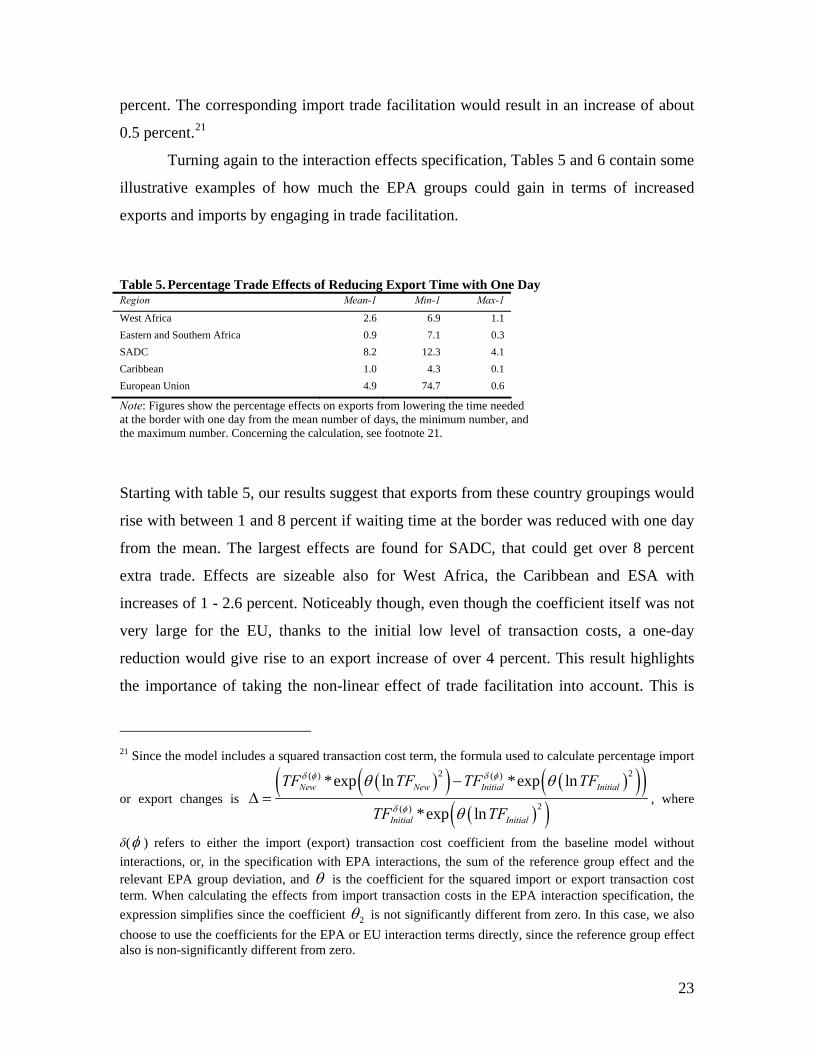
Turning again to the interaction effects specification, Tables 5 and 6 contain some
illustrative examples of how much the EPA groups could gain in terms of increased
exports and imports by engaging in trade facilitation.
Table 5. Percentage Trade Effects of Reducing Export Time with One Day Region Mean-1 Min-1 Max-1
West Africa 2.6 6.9 1.1 Eastern and Southern Africa 0.9 7.1 0.3 SADC 8.2 12.3 4.1 Caribbean 1.0 4.3 0.1 European Union 4.9 74.7 0.6
Note: Figures show the percentage effects on exports from lowering the time needed at the border with one day from the mean number of days, the minimum number, and the maximum number. Concerning the calculation, see footnote 21.
Starting with table 5, our results suggest that exports from these country groupings would
rise with between 1 and 8 percent if waiting time at the border was reduced with one day
from the mean. The largest effects are found for SADC, that could get over 8 percent
extra trade. Effects are sizeable also for West Africa, the Caribbean and ESA with
increases of 1 - 2.6 percent. Noticeably though, even though the coefficient itself was not
very large for the EU, thanks to the initial low level of transaction costs, a one-day
reduction would give rise to an export increase of over 4 percent. This result highlights
the importance of taking the non-linear effect of trade facilitation into account. This is
21 Since the model includes a squared transaction cost term, the formula used to calculate percentage import
or export changes is ( )( ) ( )( )( )
( )( )2 2( ) ( )
2( )
*exp ln *exp ln
*exp ln
New New Initial Initial
Initial Initial
TF TF TF TF
TF TF
δ φ δ φ
δ φ
θ θ
θ
−Δ = , where
δ(φ ) refers to either the import (export) transaction cost coefficient from the baseline model without interactions, or, in the specification with EPA interactions, the sum of the reference group effect and the relevant EPA group deviation, and θ is the coefficient for the squared import or export transaction cost term. When calculating the effects from import transaction costs in the EPA interaction specification, the expression simplifies since the coefficient 2θ is not significantly different from zero. In this case, we also choose to use the coefficients for the EPA or EU interaction terms directly, since the reference group effect also is non-significantly different from zero.
23
further illustrated in columns two and three, where it is evident that countries that already
have small border delays would get larger effects from reducing them with one day.
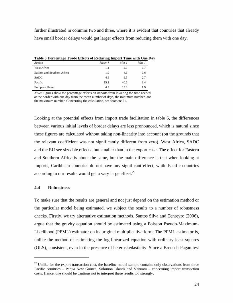
Table 6. Percentage Trade Effects of Reducing Import Time with One Day Region Mean-1 Min-1 Max-1
West Africa 1.1 2.3 0.7 Eastern and Southern Africa 1.0 4.5 0.6 SADC 4.9 9.5 2.7 Pacific 15.1 40.6 8.4 European Union 4.3 15.0 1.9
Note: Figures show the percentage effects on imports from lowering the time needed at the border with one day from the mean number of days, the minimum number, and the maximum number. Concerning the calculation, see footnote 21.
Looking at the potential effects from import trade facilitation in table 6, the differences
between various initial levels of border delays are less pronounced, which is natural since
these figures are calculated without taking non-linearity into account (on the grounds that
the relevant coefficient was not significantly different from zero). West Africa, SADC
and the EU see sizeable effects, but smaller than in the export case. The effect for Eastern
and Southern Africa is about the same, but the main difference is that when looking at
imports, Caribbean countries do not have any significant effect, while Pacific countries
according to our results would get a vary large effect.22
4.4 Robustness
To make sure that the results are general and not just depend on the estimation method or
the particular model being estimated, we subject the results to a number of robustness
checks. Firstly, we try alternative estimation methods. Santos Silva and Tenreyro (2006),
argue that the gravity equation should be estimated using a Poisson Pseudo-Maximum-
Likelihood (PPML) estimator on its original multiplicative form. The PPML estimator is,
unlike the method of estimating the log-linearized equation with ordinary least squares
(OLS), consistent, even in the presence of heteroskedasticity. Since a Breusch-Pagan test
22 Unlike for the export transaction cost, the baseline model sample contains only observations from three Pacific countries – Papua New Guinea, Solomon Islands and Vanuatu – concerning import transaction costs. Hence, one should be cautious not to interpret these results too strongly.
24
for heteroskedasticity suggests that this might indeed be a problem, we try estimating
with the PPML estimator on the gravity equation in its multiplicative form.23 The results
are displayed in table 9. We consider the Poisson estimation to be the main alternative to
a sample selection process, so the model is estimated both with (column 3) and without
(column 4) interaction terms for EPA groups.
Further, as noted by Djankov, Freund and Pham (2006), endogeneity might be a
concern, since trade volumes might not only be affected by border delays, but also in its
turn affect waiting time. For instance, large trade volumes might cause congestion, thus
intensifying the problems with inefficient procedures, or, it could on the other hand put
more pressure on the government to actually use efficient procedures. To see whether this
affects our results, we estimate the model with IV estimation, using the number of
documents needed for exports and imports and the level of corruption in the exporting
and importing country as instruments for the trade transaction variables.24 The results are
shown in column 5 of table 9.
As noted above, Helpman, Melitz and Rubinstein (2007) argue that when
estimating the gravity equation, one should not only control for sample selection, which
the ordinary Heckman procedure does, but also for the fraction of exporting firms. We
use their proposed estimation strategy (from now on the HMR approach), but unlike
them, we do not estimate the second stage non-linear equation with maximum likelihood,
but choose to use non-linear least squares. The results are shown in column 6.
Reassuringly, for almost all variables, the results are the same regardless of
estimation method. Looking specifically at the transaction cost variables, export
transaction costs have a very robust negative significant effect on trade flows, and the
squared term is also robustly positively significant. Results for import transaction costs
are somewhat less robust: ignoring for now the specification with interaction terms, the
import transaction cost coefficient is negative and significant using Heckman, IV and the
23 Santos Silva and Tenreyro (2006) note that for the PPML estimator to be consistent, the data do not have to be Poisson distributed, and in fact, the dependent variable does not even have to be an integer. The model is estimated on the original multiplicative form of the model using STATA’s poisson command with robust standard errors. 24 These variables are less likely to be influenced by trade flows. The model is estimated using STATA’s ivreg2 command with robust standard errors. We find it difficult to instrument for all interaction terms, so we use the model with only average effects for all countries.
25
HMR approach, but not using Poisson estimation. The corresponding squared term is
always positive, but only significant using Heckman or HMR. This suggests firstly that
one may be slightly more confident regarding the export transaction costs results, and
secondly that even if endogeneity is a problem, taking it into account does not alter any
results in a fundamental way.
Looking also at the results for the EPA interaction terms, table 10 reproduces
table 4, but also includes the same coefficients estimated with Poisson. Here, it is evident
that even though the magnitude of the coefficients might differ, in almost all cases the
qualitative conclusions are the same. The only exceptions to this rule is that in the
Poisson estimation, all EPA groups and the EU have significant, negative total effects
from export transaction costs, while Central Africa and the Pacific do not in the Heckman
estimation, and further that the EU does not have any negative effect from import
transaction costs in the Poisson regression. This further strengthens the conclusion that
our results are general: even though the average effect of import transaction costs is not
significant with a Poisson estimation, the effects for our regions of special interest is very
similar also when using Poisson.
Besides estimation methods, another important robustness check is to make sure
that the conclusions are not the results of one single model specification. Since adding
more variables nearly always leads to a loss of observations – especially in a developing
country context – we choose to keep the baseline model parsimonious, but in table 11 in
the Appendix, the model is estimated with various additional control variables.
To make sure that our trade facilitation variables are not picking up wider aspects
of trade costs, we follow Wilson, Mann and Otsuki (2005) and include separate measures
for what they call port efficiency, regulatory environment, and service sector
infrastructure. In the first category, they include indices of port facilities and inland
waterways plus air transport. The closest thing we can come to this without loosing
unacceptably many observations is to include the number of aircraft departures. In the
second category Wilson, Mann and Otsuki include transparency of government policy
and control of corruption. We include control of corruption. Lastly, Wilson, Mann and
Otsuki include speed and cost of internet access and effect of internet on business as
26
measures of service sector infrastructure. We include the similar number of internet users
per 1000 people.
We also include the proportion of GDP coming from agriculture. The reason for
this is that our measures for cross-border transaction costs really only apply to a certain
standardized good that is not very time-sensitive. Agricultural exports are likely more
time-sensitive, which means that problems with long waiting at the border could be worse
for agricultural exporters. We also try including the share of exports and imports
respectively from the US, again as a way to control for the content of trade.
Including these extra control variables generally does very little to alter the
results. With the only exception of the squared export transaction cost variable that
becomes insignificant in the specification including control of corruption, all results for
the transaction cost variables remain the same. Control of corruption further has the
expected positive coefficient: less corrupt countries both export and import more. Besides
this, the only additional variable that has a significant effect is share of agriculture in
GDP: having a large agricultural sector is associated with larger imports.
The conclusions we draw from these robustness tests are that our model and
results are quite robust to both alternative estimation approaches and different
specifications, and that our conclusions regarding the specific effects on EPA groups also
seem to hold. In fact, our estimation strategy reassuringly seems to be both robust and
conservative, in that in all almost cases for which it yields significant effects, the main
alternative of Poisson estimation also yields the same result, but the latter generally
suggest larger effects and also significance in some extra cases. This suggests that we
may be fairly confident about the results we find. It should be borne in mind though that
the average results for export transaction costs seem more robust than those for import
transaction costs: the latter are significant with three of our estimation choices, but not
using Poisson estimation.
27
5 Conclusions
In this paper, we have assessed how large effects export and import transaction costs
related to cross-border trade procedures have on trade flows on average and hence how
big the potential benefits from trade facilitation are. We have further also estimated these
effects separately for EPA negotiating groups and for the EU. Using data from the World
Bank’s (2007) Doing Business Database on the time required to export or import as
indicators of trade transaction costs, we have estimated a gravity model on two-way
bilateral trade between EU countries and developing countries using a sample selection
approach.
We find that time delays both on the part of the exporter and the importer,
proxying export and import transaction costs, on average significantly decrease trade
flows. We also find that this relationship is not linear: an extra day of waiting has smaller
marginal effects if the time requirements are already high. The effects of export
transaction costs are larger. On average, lowering border delays in the exporting country
with one day (from the sample mean) would yield an export increasing effect of about 1
percent, while the same reduction in the importing country would give an import increase
of about 0.5 percent.
Moreover, countries negotiating in the EPA groups for SADC, West Africa,
Eastern and Southern Africa, and the Caribbean have negative and significant effects
from export transaction costs, as do EU and non-ACP developing countries. The effects
for the SADC, West African and ESA groups are the largest. Reducing border delays
with one day from the within-group mean would increase exports with between 1 and 8
percent. The results are somewhat different for import transaction costs, where countries
in the Pacific, SADC, West Africa and the EU have significantly negative effects from
import transaction costs, with the effects being the largest for the two former groups. The
percentage effects of reducing import border delays with one day are generally of the
same magnitude as those for export border delays, with the exception of the Pacific
countries, where results suggest increases of around 15 percent.
Concerning the average effects of trade facilitation, our results confirm the
conclusions drawn by Djankov, Fruend and Pham (2006), Nordås, Pinali and Grosso
28

(2006) and Soloaga, Wilson and Mejía (2006) that export trade facilitation have positive
potential effects, and the magnitude of these effects closely resemble those suggested by
Djankov, Freund and Pham (2006). Estimations of the potential effects of import trade
facilitation have been rarer in the literature, but our results do confirm those obtained by
Wilson, Mann and Otsuki (2003; 2005). Our results highlight a number of issues though.
Firstly, they illustrate the importance of including indicators for trade facilitation in both
the exporting and the importing country: inefficient border procedures matter, regardless
or where they occur. Secondly, our results clearly suggest that the effect of cumbersome
border procedures is not linear, so a failure to take this into account can risk biasing ones
results. This will be particularly important when analysing the policy implications of
trade facilitation reforms. Thirdly, and related to this, it seems to be important to allow
the effects of trade facilitation to differ for country groups. By just estimating one
average effect and then using this to calculate potential trade impact of reform, one will
run a serious risk of drawing misleading conclusions.
To draw some policy conclusions, our results suggest that there are indeed
positive gains to be won by making it simpler for goods to cross borders. This general
conclusion also holds for most, though not necessarily all, EPA groups. For some, gains
would even be considerably larger than for the average country. Obviously, reforming
the customs environment can entail certain costs, but compared with other areas of
negotiation in the current discussions with the EU about EPAs, at least the benefits from
trade facilitation are clear and sizeable. It is important to note, though, that the potential
benefits from trade facilitation are not necessarily tied to the EPA framework: the
relevant countries could increase their trade unilaterally by engaging in their own reform.
Since trade facilitation has positive effects both when it is performed at the origin and at
the destination, an agreement about mutual reforms would, however, yield larger
potential gains. If ACP countries e.g. aim to increase their exports, one way of doing this
would be through EU import trade facilitation. This emphasizes the importance of
reaching an agreement. Moreover, since trade facilitation can involve not only
simplification but also harmonization, one could argue that EPA countries perhaps have a
better chance of influencing which standards one is to harmonize around through
negotiations, rather than just unilateral reform.
29
References
ACP Council of Ministers (2002), “ACP Guidelines for the Negotiations of Economic
Partnership Agreements”, ACP/61/056/02 [FINAL].
Anderson, James E. (1979), “A Theoretical Foundation for the Gravity Equation”, American
Economic Review, Vol. 69, No. 1, pp. 106-116.
Anderson, James E. and Eric van Wincoop (2003), “Gravity with Gravitas: A Solution to the
Border Puzzle”, American Economic Review, Vol. 93, No. 1, pp. 170-192.
Anderson, James E. and Eric van Wincoop (2004), “Trade Costs”, Journal of Economic
Literature, Vol. 42, No. 3, pp. 691-751.
Bergstrand, Jeffrey H (1985), “The Gravity Equation in International Trade: Some
Microeconomic Foundations and Empirical Evidence”, Review of Economics and Statistics,
Vol. 67, No. 3, pp. 474-481.
Bergstrand, Jeffrey H. (1989), “The Generalized Gravity Equation, Monopolistic Competition,
and the Factor-Proportions Theory in International Trade”, Review of Economics and
Statistics, Vol. 71, No. 1, pp. 143-153.
Bouët, Antoine, Yvan Decreux, Lionel Fontagné, Sébastien Jean and David Laborde (2004), “A
Consistent, Ad-Valorem Equivalent Measure of Applied Protection Across the World : The
MAcMap-HS6 Database”, CEPII Working Paper No. 2004-22.
CEPII (2006), “Distances”, http://www.cepii.fr/anglaisgraph/bdd/distances.htm.
CEPII (2007), “HS2 Aggregation: Applied rates from MAcMap HS6 v1.1 and Bound Tariffs”,
http://www.cepii.fr/anglaisgraph/bdd/macmap/form_macpmap/download.asp.
Deardorff, Alan V. (1998), “Determinants of Bilateral Trade: Does Gravity Work in a
Neoclassical World”, in J. A. Frankel (ed.), The Regionalization of the World Economy.
Chicago: University of Chicago Press, pp. 7-22.
Decreux, Yvan and Lionel Fontagné (2006), “A Quantitative Assessment of the Outcome of the
Doha Development Agenda”, CEPII Working Paper No. 2006-10.
Dennis, Allen (2006), “The Impact of Regional Trade Agreements and Trade Facilitation in the
Middle East North Africa Region”, World Bank Policy Research Working Paper No. 3837.
Djankov, Simeon, Caroline Freund and Cong S. Pham (2006), “Trading on Time”, World Bank
Policy Research Working Paper No. 3909.
ECDPM (2006), “Overview of the Regional EPA Negotiations: West Africa-EU Economic
Partnership Agreement”, ECDPM InBrief 14B, Maastricht: www.ecdpm.org/inbrief14b.
30
Engman, Michael (2005), “The Economic Impact of Trade Facilitation”, OECD Trade Policy
Working Paper, No. 21.
European Commission (2002), “Explanatory Memorandum. Commission Draft Mandate 9 April
2002”, http://trade.ec.europa.eu/doclib/docs/2006/september/tradoc_112023.pdf.
European Commission (2006), http://ec.europa.eu/comm/external_relations/.
European Commission (2007a), “Economic Partnership Agreements (EPAs). Negotiations: A
New Approach to ACP-EU Trade Cooperation”,
http://ec.europa.eu/trade/issues/bilateral/regions/acp/epas.htm.
European Commission (2007b), “The EU Welcomes South Africa in the SADC EPA
negotiation”,
http://ec.europa.eu/trade/issues/bilateral/countries/southafrica/pr140207_en.htm
Francois, Joseph, Hans van Meijl and Frank van Tongeren (2005), “Trade Liberalization in the
Doha Development Round”, Economic Policy, Vol. 20, No. 42, pp. 349-391.
Greenaway, David and Chris Milner (2002), “Regionalism and Gravity”, Scottish Journal of
Political Economy, Vol. 49, No. 5, pp. 574-585.
Helpman, Elhanan and Paul R. Krugman (1985), Market Structure and Foreign Trade,
Cambridge, Massachusetts: MIT Press.
Helpman, Elhanan, Marc J. Melitz and Yona Rubinstein (2007), “Estimating Trade Flows:
Trading Partners and Trading Volumes”, NBER Working Paper No. 12927.
Hertel, Thomas W. and Roman Keeney (2006), “What is at Stake: The Relative Importance of
Import Barriers, Export Subsidies, and Domestic Support”, in Kym Anderson and Will
Martin (eds.), Agricultural Trade Reform & the Doha Development Agenda, Washington
D.C.: The World Bank and Hampshire and New York: Palgrave Macmillan, pp. 37-62.
Hinkle, Lawrence, Mombert Hoppe and Richard Newfarmer (2006), “Beyond Cotonou:
Economic Partnership Agreements in Africa”, in Richard Newfarmer, (ed.), Trade, Doha,
and Development: A Window into the Issues, Washington, D.C.: The World Bank, pp. 263-
276.
Hummels, David (2001), “Time as a Trade Barrier”, mimeo, Purdue University.
IMF (2006), Direction of Trade Statistics. CD-ROM.
Melitz, Marc J. (2003), “The Impact of Trade on Intra-Industry Reallocations and Aggregate
Industry Productivity”, Econometrica, Vol 71, No. 6, pp. 1695-1725.
Nath, Kamal and Peter Mandelson (2006), “Doha Round: It’s not only what we trade, but how”,
International Herald Tribune, July 5, 2006.
31
Nordås, Hildegunn Kyvik, Enrico Pinali and Massimo Geloso Grosso (2006), “Logistics and
Time as a Trade Barrier”, OECD Trade Policy Working Paper, No. 35.
Nyamache, Nyachienga (2006), “Trade Facilitation”, EU-ACP Negotiations in Focus, Project
Management Unit, http://www.euacpepa.org:8080/index.php?page=43&lg=en.
OECD (2003), “Quantitative Assessment of the Benefits of Trade Facilitation”,
TD/TC/WP(2003)31/FINAL
Persson, Maria and Fredrik Wilhelmsson (forthcoming 2007), “Assessing the Effects of EU Trade
Preferences for Developing Countries”, in Yves Bourdet, Joakim Gullstrand and Karin
Olofsdotter (eds.): The European Union and Developing Countries: Trade, Aid and Growth
in an Integrating World. Cheltenham and Northampton: Edward Elgar, pp. 29-48.
Roy, Jayanta and Shweta Bagai (2005), “Key Issues in Trade Facilitation. Summary of World
Bank/EU Workshops in Dhaka and Shanghai in 2004”, World Bank Policy Research
Working Paper No. 3703.
Santos Silva, João M. C. and Silvana Tenreyro (2006), “The Log of Gravity”, Review of
Economics and Statistics, Vol. 88, No. 4, pp. 641-658.
Soloaga, Isidro, John S. Wilson and Alejandro Mejía (2006), “Moving Forward Faster: Trade
Facilitation Reform and Mexican Competitiveness”, World Bank Policy Research Working
Paper No. 3953.
Swedish National Board of Trade (2006), Economic Implications of the Doha Round, Stockholm.
Transparency International (2006), Corruption Perceptions Index,
http://www.icgg.org/corruption.cpi_2006.html.
Wilson, John S., Catherine L. Mann and Tsunehiro Otsuki (2003), “Trade Facilitation and
Economic Development: A New Approach to Quantifying the Impact”, World Bank
Economic Review, Vol. 17, No. 3, pp. 367-389.
Wilson, John S., Catherine L. Mann and Tsunehiro Otsuki (2005), “Assessing the Benefits of
Trade Facilitation: A Global Perspective”, World Economy, Vol. 28, No. 6, pp. 841-71.
World Bank (2006), World Development Indicators Online.
World Bank (2007), Doing Business Database,
http://www.doingbusiness.org/ExploreTopics/TradingAcrossBorders/.
WTO (2001) Ministerial Conference, Fourth Session, Doha, 9-14 November 2001, “Ministerial
Declaration”, WT/MIN(01)/DEC/1, 20 November.
WTO (2006), “Trade Facilitation”, http://www.wto.org/english/tratop_e/tradfa_e/tradfa_e.htm.
32
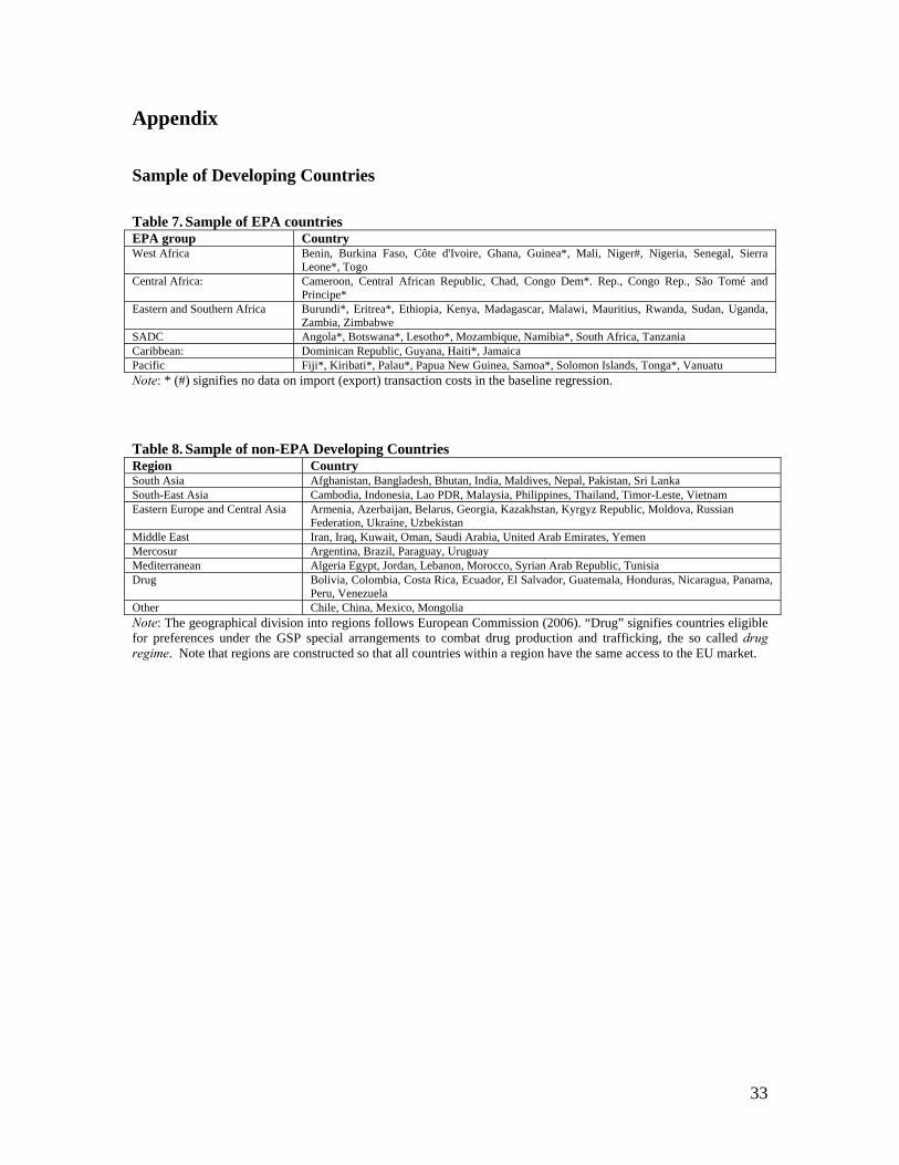
Appendix
Sample of Developing Countries
Table 7. Sample of EPA countries EPA group Country West Africa Benin, Burkina Faso, Côte d'Ivoire, Ghana, Guinea*, Mali, Niger#, Nigeria, Senegal, Sierra
Leone*, Togo Central Africa: Cameroon, Central African Republic, Chad, Congo Dem*. Rep., Congo Rep., São Tomé and
Principe* Eastern and Southern Africa Burundi*, Eritrea*, Ethiopia, Kenya, Madagascar, Malawi, Mauritius, Rwanda, Sudan, Uganda,
Zambia, Zimbabwe SADC Angola*, Botswana*, Lesotho*, Mozambique, Namibia*, South Africa, Tanzania Caribbean: Dominican Republic, Guyana, Haiti*, Jamaica Pacific Fiji*, Kiribati*, Palau*, Papua New Guinea, Samoa*, Solomon Islands, Tonga*, Vanuatu Note: * (#) signifies no data on import (export) transaction costs in the baseline regression.
Table 8. Sample of non-EPA Developing Countries Region Country South Asia Afghanistan, Bangladesh, Bhutan, India, Maldives, Nepal, Pakistan, Sri Lanka South-East Asia Cambodia, Indonesia, Lao PDR, Malaysia, Philippines, Thailand, Timor-Leste, Vietnam Eastern Europe and Central Asia Armenia, Azerbaijan, Belarus, Georgia, Kazakhstan, Kyrgyz Republic, Moldova, Russian
Federation, Ukraine, Uzbekistan Middle East Iran, Iraq, Kuwait, Oman, Saudi Arabia, United Arab Emirates, Yemen Mercosur Argentina, Brazil, Paraguay, Uruguay Mediterranean Algeria Egypt, Jordan, Lebanon, Morocco, Syrian Arab Republic, Tunisia Drug Bolivia, Colombia, Costa Rica, Ecuador, El Salvador, Guatemala, Honduras, Nicaragua, Panama,
Peru, Venezuela Other Chile, China, Mexico, Mongolia Note: The geographical division into regions follows European Commission (2006). “Drug” signifies countries eligible for preferences under the GSP special arrangements to combat drug production and trafficking, the so called drug regime. Note that regions are constructed so that all countries within a region have the same access to the EU market.
33
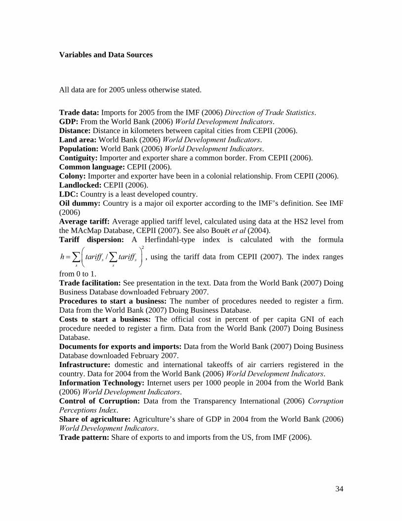
34
2
/s ss s
h tariff tariff⎛ ⎞= ⎜ ⎟⎝ ⎠
∑ ∑
Variables and Data Sources
All data are for 2005 unless otherwise stated.
Trade data: Imports for 2005 from the IMF (2006) Direction of Trade Statistics. GDP: From the World Bank (2006) World Development Indicators. Distance: Distance in kilometers between capital cities from CEPII (2006). Land area: World Bank (2006) World Development Indicators. Population: World Bank (2006) World Development Indicators. Contiguity: Importer and exporter share a common border. From CEPII (2006). Common language: CEPII (2006). Colony: Importer and exporter have been in a colonial relationship. From CEPII (2006). Landlocked: CEPII (2006). LDC: Country is a least developed country. Oil dummy: Country is a major oil exporter according to the IMF’s definition. See IMF (2006) Average tariff: Average applied tariff level, calculated using data at the HS2 level from the MAcMap Database, CEPII (2007). See also Bouët et al (2004). Tariff dispersion: A Herfindahl-type index is calculated with the formula
, using the tariff data from CEPII (2007). The index ranges
from 0 to 1. Trade facilitation: See presentation in the text. Data from the World Bank (2007) Doing Business Database downloaded February 2007. Procedures to start a business: The number of procedures needed to register a firm. Data from the World Bank (2007) Doing Business Database. Costs to start a business: The official cost in percent of per capita GNI of each procedure needed to register a firm. Data from the World Bank (2007) Doing Business Database. Documents for exports and imports: Data from the World Bank (2007) Doing Business Database downloaded February 2007. Infrastructure: domestic and international takeoffs of air carriers registered in the country. Data for 2004 from the World Bank (2006) World Development Indicators. Information Technology: Internet users per 1000 people in 2004 from the World Bank (2006) World Development Indicators. Control of Corruption: Data from the Transparency International (2006) Corruption Perceptions Index. Share of agriculture: Agriculture’s share of GDP in 2004 from the World Bank (2006) World Development Indicators. Trade pattern: Share of exports to and imports from the US, from IMF (2006).
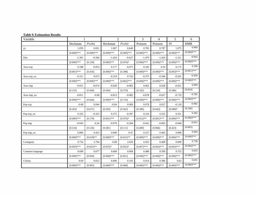
Table 9. Estimation Results Variable 1 2 3 4 5 6 Heckman Probit Heckman Probit Poisson Poisson IV HMR yy 1.059 0.651 1.067 0.648 0.783 0.787 1.075 0.909
[0.000]*** [0.000]*** [0.000]*** [0.000]*** [0.000]*** [0.000]*** [0.000]*** [0.000]***
Dist -1.301 -0.566 -1.424 -0.627 -1.479 -1.424 -1.311 -0.942
[0.000]*** [0.139] [0.000]*** [0.076]* [0.000]*** [0.000]*** [0.000]*** [0.000]***
Area exp 0.188 -0.053 0.177 -0.075 0.245 0.24 0.175 0.196
[0.001]*** [0.416] [0.006]*** [0.398] [0.000]*** [0.000]*** [0.003]*** [0.001]***
Area exp_eu -0.311 0.673 -0.319 0.743 -0.375 -0.346 -0.261 -0.459
[0.000]*** [0.006]*** [0.000]*** [0.002]*** [0.000]*** [0.000]*** [0.000]*** [0.000]***
Area imp -0.051 -0.074 -0.028 -0.082 0.062 0.028 -0.021 0.009
[0.155] [0.560] [0.566] [0.579] [0.182] [0.524] [0.586] [0.824]
Area imp_eu -0.811 -0.08 -0.813 -0.082 -0.678 -0.637 -0.719 -0.785
[0.000]*** [0.644] [0.000]*** [0.710] [0.000]*** [0.000]*** [0.000]*** [0.000]***
Pop exp -0.08 0.044 -0.04 0.069 0.078 0.037 -0.118 -0.082
[0.262] [0.671] [0.595] [0.562] [0.396] [0.643] [0.098]* [0.240]
Pop exp_eu 0.335 -0.323 0.275 -0.397 0.224 0.255 0.351 0.382
[0.000]*** [0.179] [0.001]*** [0.076]* [0.012]** [0.001]*** [0.000]*** [0.000]***
Pop imp -0.045 -0.26 -0.079 -0.284 -0.041 -0.003 -0.048 -0.031
[0.516] [0.126] [0.281] [0.111] [0.490] [0.966] [0.423] [0.603]
Pop imp_eu 0.806 0.423 0.849 0.47 0.527 0.465 0.808 0.684
[0.000]*** [0.018]** [0.000]*** [0.031]** [0.000]*** [0.000]*** [0.000]*** [0.000]***
Contiguity 0.754 2.794 0.68 2.634 0.425 0.469 0.909 0.758
[0.003]*** [0.025]** [0.055]* [0.055]* [0.007]*** [0.003]*** [0.003]*** [0.004]***
Common language 0.698 0.077 0.668 0.094 0.488 0.509 0.732 0.653
[0.000]*** [0.850] [0.000]*** [0.821] [0.000]*** [0.000]*** [0.000]*** [0.000]***
Colony 0.69 0.022 0.696 0.102 0.414 0.386 0.63 0.691
[0.000]*** [0.993] [0.000]*** [0.968] [0.000]*** [0.000]*** [0.000]*** [0.000]***
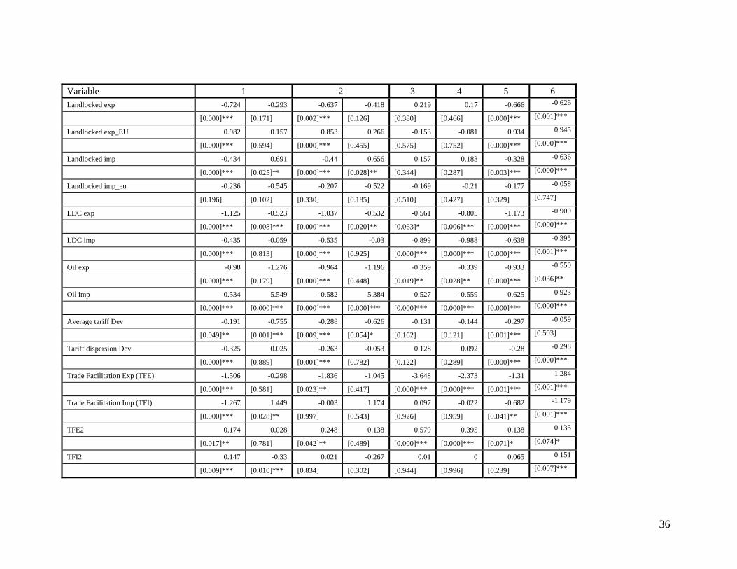
Variable 1 2 3 4 5 6 Landlocked exp -0.724 -0.293 -0.637 -0.418 0.219 0.17 -0.666 -0.626
[0.000]*** [0.171] [0.002]*** [0.126] [0.380] [0.466] [0.000]*** [0.001]***
Landlocked exp_EU 0.982 0.157 0.853 0.266 -0.153 -0.081 0.934 0.945
[0.000]*** [0.594] [0.000]*** [0.455] [0.575] [0.752] [0.000]*** [0.000]***
Landlocked imp -0.434 0.691 -0.44 0.656 0.157 0.183 -0.328 -0.636
[0.000]*** [0.025]** [0.000]*** [0.028]** [0.344] [0.287] [0.003]*** [0.000]***
Landlocked imp_eu -0.236 -0.545 -0.207 -0.522 -0.169 -0.21 -0.177 -0.058
[0.196] [0.102] [0.330] [0.185] [0.510] [0.427] [0.329] [0.747]
LDC exp -1.125 -0.523 -1.037 -0.532 -0.561 -0.805 -1.173 -0.900
[0.000]*** [0.008]*** [0.000]*** [0.020]** [0.063]* [0.006]*** [0.000]*** [0.000]***
LDC imp -0.435 -0.059 -0.535 -0.03 -0.899 -0.988 -0.638 -0.395
[0.000]*** [0.813] [0.000]*** [0.925] [0.000]*** [0.000]*** [0.000]*** [0.001]***
Oil exp -0.98 -1.276 -0.964 -1.196 -0.359 -0.339 -0.933 -0.550
[0.000]*** [0.179] [0.000]*** [0.448] [0.019]** [0.028]** [0.000]*** [0.036]**
Oil imp -0.534 5.549 -0.582 5.384 -0.527 -0.559 -0.625 -0.923
[0.000]*** [0.000]*** [0.000]*** [0.000]*** [0.000]*** [0.000]*** [0.000]*** [0.000]***
Average tariff Dev -0.191 -0.755 -0.288 -0.626 -0.131 -0.144 -0.297 -0.059
[0.049]** [0.001]*** [0.009]*** [0.054]* [0.162] [0.121] [0.001]*** [0.503]
Tariff dispersion Dev -0.325 0.025 -0.263 -0.053 0.128 0.092 -0.28 -0.298
[0.000]*** [0.889] [0.001]*** [0.782] [0.122] [0.289] [0.000]*** [0.000]***
Trade Facilitation Exp (TFE) -1.506 -0.298 -1.836 -1.045 -3.648 -2.373 -1.31 -1.284
[0.000]*** [0.581] [0.023]** [0.417] [0.000]*** [0.000]*** [0.001]*** [0.001]***
Trade Facilitation Imp (TFI) -1.267 1.449 -0.003 1.174 0.097 -0.022 -0.682 -1.179
[0.000]*** [0.028]** [0.997] [0.543] [0.926] [0.959] [0.041]** [0.001]***
TFE2 0.174 0.028 0.248 0.138 0.579 0.395 0.138 0.135
[0.017]** [0.781] [0.042]** [0.489] [0.000]*** [0.000]*** [0.071]* [0.074]*
TFI2 0.147 -0.33 0.021 -0.267 0.01 0 0.065 0.151
[0.009]*** [0.010]*** [0.834] [0.302] [0.944] [0.996] [0.239] [0.007]***
36
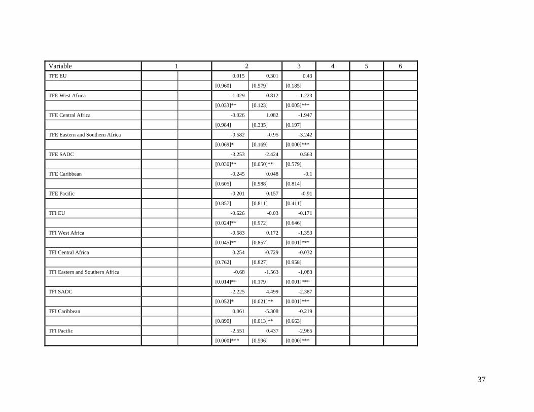
Variable 1 2 3 4 5 6 TFE EU 0.015 0.301 0.43
[0.960] [0.579] [0.185]
TFE West Africa -1.029 0.812 -1.223
[0.033]** [0.123] [0.005]***
TFE Central Africa -0.026 1.082 -1.947
[0.984] [0.335] [0.197]
TFE Eastern and Southern Africa -0.582 -0.95 -3.242
[0.069]* [0.169] [0.000]***
TFE SADC -3.253 -2.424 0.563
[0.030]** [0.050]** [0.579]
TFE Caribbean -0.245 0.048 -0.1
[0.605] [0.988] [0.814]
TFE Pacific -0.201 0.157 -0.91
[0.857] [0.811] [0.411]
TFI EU -0.626 -0.03 -0.171
[0.024]** [0.972] [0.646]
TFI West Africa -0.583 0.172 -1.353
[0.045]** [0.857] [0.001]***
TFI Central Africa 0.254 -0.729 -0.032
[0.762] [0.827] [0.958]
TFI Eastern and Southern Africa -0.68 -1.563 -1.083
[0.014]** [0.179] [0.001]***
TFI SADC -2.225 4.499 -2.387
[0.052]* [0.021]** [0.001]***
TFI Caribbean 0.061 -5.308 -0.219
[0.890] [0.013]** [0.663]
TFI Pacific -2.551 0.437 -2.965
[0.000]*** [0.596] [0.000]***
37
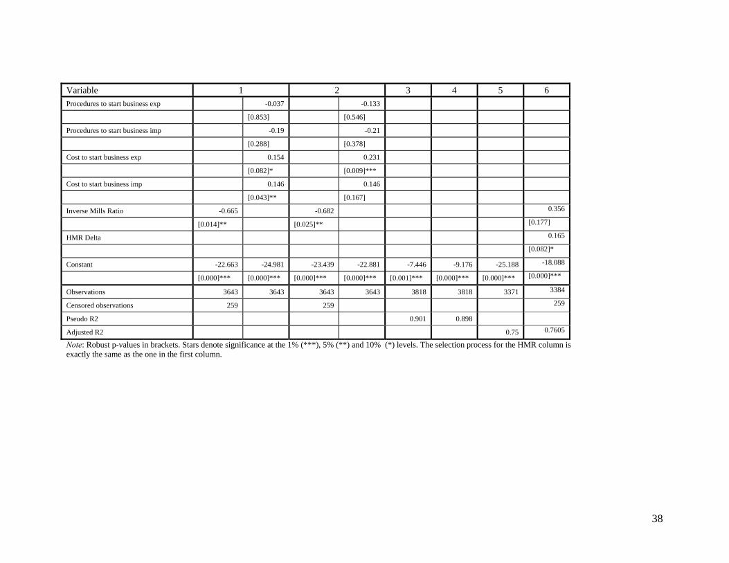
Variable 1 2 3 4 5 6 Procedures to start business exp -0.037 -0.133
[0.853] [0.546]
Procedures to start business imp -0.19 -0.21
[0.288] [0.378]
Cost to start business exp 0.154 0.231
[0.082]* [0.009]***
Cost to start business imp 0.146 0.146
[0.043]** [0.167]
Inverse Mills Ratio -0.665 -0.682 0.356
[0.014]** [0.025]** [0.177]
HMR Delta 0.165
[0.082]*
Constant -22.663 -24.981 -23.439 -22.881 -7.446 -9.176 -25.188 -18.088
[0.000]*** [0.000]*** [0.000]*** [0.000]*** [0.001]*** [0.000]*** [0.000]*** [0.000]***
Observations 3643 3643 3643 3643 3818 3818 3371 3384
Censored observations 259 259 259
Pseudo R2 0.901 0.898
Adjusted R2 0.75 0.7605
Note: Robust p-values in brackets. Stars denote significance at the 1% (***), 5% (**) and 10% (*) levels. The selection process for the HMR column is exactly the same as the one in the first column.
38
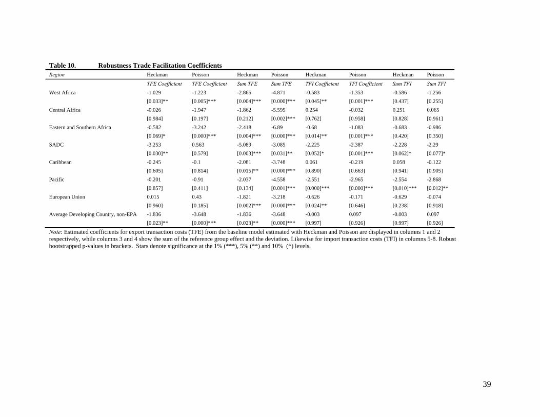
Table 10. Robustness Trade Facilitation Coefficients Region Heckman Poisson Heckman Poisson Heckman Poisson Heckman Poisson
TFE Coefficient TFE Coefficient Sum TFE Sum TFE TFI Coefficient TFI Coefficient Sum TFI Sum TFI West Africa -1.029 -1.223 -2.865 -4.871 -0.583 -1.353 -0.586 -1.256 [0.033]** [0.005]*** [0.004]*** [0.000]*** [0.045]** [0.001]*** [0.437] [0.255] Central Africa -0.026 -1.947 -1.862 -5.595 0.254 -0.032 0.251 0.065 [0.984] [0.197] [0.212] [0.002]*** [0.762] [0.958] [0.828] [0.961] Eastern and Southern Africa -0.582 -3.242 -2.418 -6.89 -0.68 -1.083 -0.683 -0.986 [0.069]* [0.000]*** [0.004]*** [0.000]*** [0.014]** [0.001]*** [0.420] [0.350] SADC -3.253 0.563 -5.089 -3.085 -2.225 -2.387 -2.228 -2.29 [0.030]** [0.579] [0.003]*** [0.031]** [0.052]* [0.001]*** [0.062]* [0.077]* Caribbean -0.245 -0.1 -2.081 -3.748 0.061 -0.219 0.058 -0.122 [0.605] [0.814] [0.015]** [0.000]*** [0.890] [0.663] [0.941] [0.905] Pacific -0.201 -0.91 -2.037 -4.558 -2.551 -2.965 -2.554 -2.868 [0.857] [0.411] [0.134] [0.001]*** [0.000]*** [0.000]*** [0.010]*** [0.012]** European Union 0.015 0.43 -1.821 -3.218 -0.626 -0.171 -0.629 -0.074 [0.960] [0.185] [0.002]*** [0.000]*** [0.024]** [0.646] [0.238] [0.918] Average Developing Country, non-EPA -1.836 -3.648 -1.836 -3.648 -0.003 0.097 -0.003 0.097 [0.023]** [0.000]*** [0.023]** [0.000]*** [0.997] [0.926] [0.997] [0.926]
Note: Estimated coefficients for export transaction costs (TFE) from the baseline model estimated with Heckman and Poisson are displayed in columns 1 and 2 respectively, while columns 3 and 4 show the sum of the reference group effect and the deviation. Likewise for import transaction costs (TFI) in columns 5-8. Robust bootstrapped p-values in brackets. Stars denote significance at the 1% (***), 5% (**) and 10% (*) levels.
39
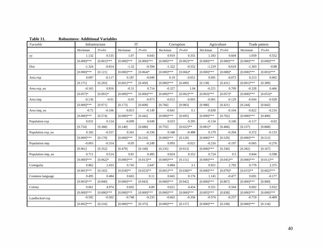
Table 11. Robustness: Additional Variables Variable Infrastructure IT Corruption Agriculture Trade pattern Heckman Probit Heckman Probit Heckman Probit Heckman Probit Heckman Probit
yy 1.132 0.535 1.07 0.643 0.919 0.355 1.183 0.604 1.059 0.552
[0.000]*** [0.001]*** [0.000]*** [0.000]*** [0.000]*** [0.002]*** [0.000]*** [0.000]*** [0.000]*** [0.000]***
Dist -1.324 -0.814 -1.32 -0.594 -1.322 -0.552 -1.219 -0.619 -1.303 -0.88
[0.000]*** [0.121] [0.000]*** [0.064]* [0.000]*** [0.066]* [0.000]*** [0.088]* [0.000]*** [0.003]***
Area exp 0.097 -0.117 0.187 -0.049 0.19 -0.051 0.091 -0.072 0.213 0.065
[0.171] [0.293] [0.001]*** [0.450] [0.000]*** [0.499] [0.138] [0.431] [0.001]*** [0.389]
Area exp_eu -0.165 0.816 -0.31 0.714 -0.327 1.04 -0.221 0.709 -0.328 0.466
[0.057]* [0.091]* [0.000]*** [0.006]*** [0.000]*** [0.002]*** [0.003]*** [0.057]* [0.000]*** [0.053]*
Area imp -0.136 -0.01 -0.05 -0.073 -0.012 -0.003 -0.001 -0.129 -0.044 -0.028
[0.000]*** [0.971] [0.173] [0.608] [0.766] [0.983] [0.986] [0.421] [0.244] [0.842]
Area imp_eu -0.72 -0.166 -0.815 -0.149 -0.841 0.1 -0.838 -0.104 -0.822 -0.216
[0.000]*** [0.574] [0.000]*** [0.442] [0.000]*** [0.695] [0.000]*** [0.702] [0.000]*** [0.400]
Population exp 0.031 0.154 -0.099 0.049 0.023 0.395 -0.134 0.106 -0.117 -0.02
[0.724] [0.368] [0.140] [0.686] [0.755] [0.022]** [0.081]* [0.484] [0.157] [0.868]
Population exp_eu 0.182 -0.557 0.341 -0.336 0.348 -0.488 0.179 -0.204 0.372 -0.133
[0.009]*** [0.179] [0.000]*** [0.210] [0.000]*** [0.120] [0.006]*** [0.529] [0.000]*** [0.512]
Population imp -0.003 -0.314 -0.05 -0.249 0.093 -0.021 -0.216 -0.197 -0.065 -0.276
[0.961] [0.352] [0.479] [0.168] [0.235] [0.913] [0.006]*** [0.330] [0.282] [0.167]
Population imp_eu 0.711 0.514 0.81 0.495 0.824 0.352 0.724 0.5 0.844 0.598
[0.000]*** [0.062]* [0.000]*** [0.013]** [0.000]*** [0.151] [0.000]*** [0.045]** [0.000]*** [0.011]**
Contiguity 0.862 2.433 0.745 2.647 0.884 3.1 0.921 2.792 0.779 2.375
[0.001]*** [0.102] [0.018]** [0.023]** [0.001]*** [0.038]** [0.000]*** [0.079]* [0.015]** [0.002]***
Common language 0.495 0.484 0.665 0.11 0.665 0.176 1.145 -0.477 0.691 -0.177
[0.003]*** [0.840] [0.000]*** [0.943] [0.000]*** [0.942] [0.000]*** [0.807] [0.000]*** [0.900]
Colony 0.661 4.974 0.692 4.89 0.621 4.454 0.351 0.504 0.692 5.032
[0.000]*** [0.000]*** [0.000]*** [0.000]*** [0.000]*** [0.000]*** [0.005]*** [0.838] [0.000]*** [0.000]***
Landlocked exp -0.592 -0.502 -0.748 -0.233 -0.663 -0.356 -0.574 -0.257 -0.719 -0.409
[0.002]*** [0.216] [0.000]*** [0.375] [0.000]*** [0.157] [0.000]*** [0.238] [0.000]*** [0.134]
40
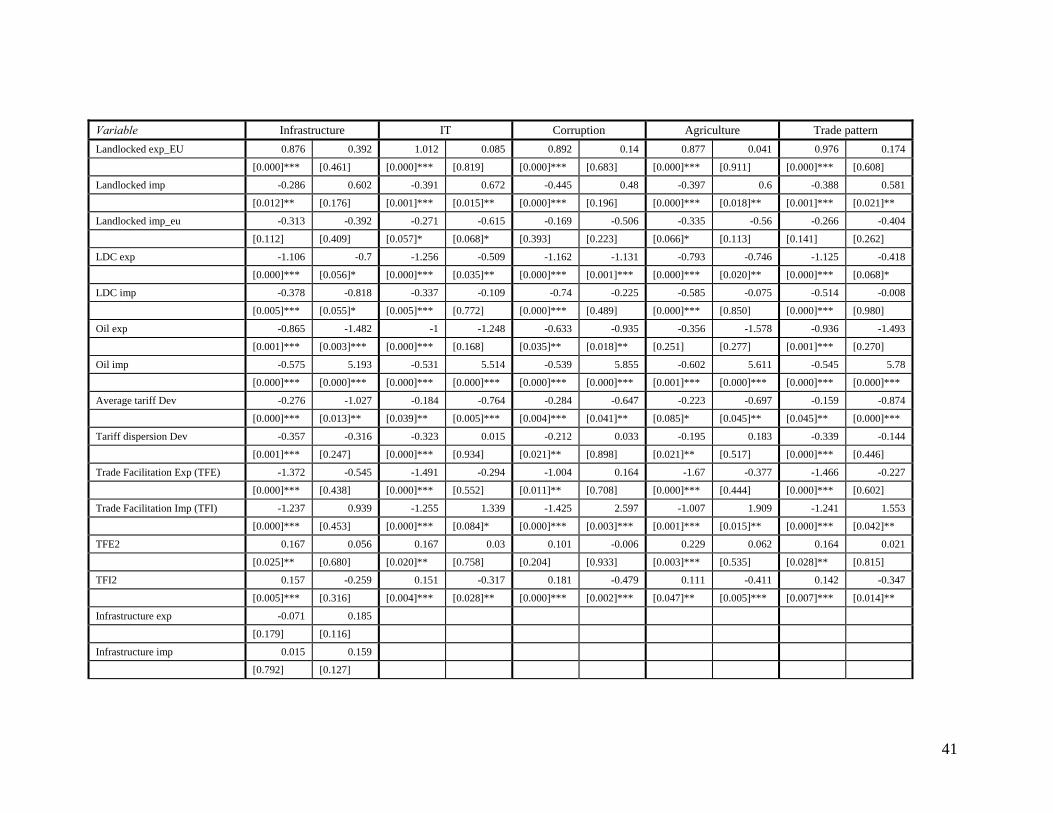
Variable Infrastructure IT Corruption Agriculture Trade pattern Landlocked exp_EU 0.876 0.392 1.012 0.085 0.892 0.14 0.877 0.041 0.976 0.174
[0.000]*** [0.461] [0.000]*** [0.819] [0.000]*** [0.683] [0.000]*** [0.911] [0.000]*** [0.608]
Landlocked imp -0.286 0.602 -0.391 0.672 -0.445 0.48 -0.397 0.6 -0.388 0.581
[0.012]** [0.176] [0.001]*** [0.015]** [0.000]*** [0.196] [0.000]*** [0.018]** [0.001]*** [0.021]**
Landlocked imp_eu -0.313 -0.392 -0.271 -0.615 -0.169 -0.506 -0.335 -0.56 -0.266 -0.404
[0.112] [0.409] [0.057]* [0.068]* [0.393] [0.223] [0.066]* [0.113] [0.141] [0.262]
LDC exp -1.106 -0.7 -1.256 -0.509 -1.162 -1.131 -0.793 -0.746 -1.125 -0.418
[0.000]*** [0.056]* [0.000]*** [0.035]** [0.000]*** [0.001]*** [0.000]*** [0.020]** [0.000]*** [0.068]*
LDC imp -0.378 -0.818 -0.337 -0.109 -0.74 -0.225 -0.585 -0.075 -0.514 -0.008
[0.005]*** [0.055]* [0.005]*** [0.772] [0.000]*** [0.489] [0.000]*** [0.850] [0.000]*** [0.980]
Oil exp -0.865 -1.482 -1 -1.248 -0.633 -0.935 -0.356 -1.578 -0.936 -1.493
[0.001]*** [0.003]*** [0.000]*** [0.168] [0.035]** [0.018]** [0.251] [0.277] [0.001]*** [0.270]
Oil imp -0.575 5.193 -0.531 5.514 -0.539 5.855 -0.602 5.611 -0.545 5.78
[0.000]*** [0.000]*** [0.000]*** [0.000]*** [0.000]*** [0.000]*** [0.001]*** [0.000]*** [0.000]*** [0.000]***
Average tariff Dev -0.276 -1.027 -0.184 -0.764 -0.284 -0.647 -0.223 -0.697 -0.159 -0.874
[0.000]*** [0.013]** [0.039]** [0.005]*** [0.004]*** [0.041]** [0.085]* [0.045]** [0.045]** [0.000]***
Tariff dispersion Dev -0.357 -0.316 -0.323 0.015 -0.212 0.033 -0.195 0.183 -0.339 -0.144
[0.001]*** [0.247] [0.000]*** [0.934] [0.021]** [0.898] [0.021]** [0.517] [0.000]*** [0.446]
Trade Facilitation Exp (TFE) -1.372 -0.545 -1.491 -0.294 -1.004 0.164 -1.67 -0.377 -1.466 -0.227
[0.000]*** [0.438] [0.000]*** [0.552] [0.011]** [0.708] [0.000]*** [0.444] [0.000]*** [0.602]
Trade Facilitation Imp (TFI) -1.237 0.939 -1.255 1.339 -1.425 2.597 -1.007 1.909 -1.241 1.553
[0.000]*** [0.453] [0.000]*** [0.084]* [0.000]*** [0.003]*** [0.001]*** [0.015]** [0.000]*** [0.042]**
TFE2 0.167 0.056 0.167 0.03 0.101 -0.006 0.229 0.062 0.164 0.021
[0.025]** [0.680] [0.020]** [0.758] [0.204] [0.933] [0.003]*** [0.535] [0.028]** [0.815]
TFI2 0.157 -0.259 0.151 -0.317 0.181 -0.479 0.111 -0.411 0.142 -0.347
[0.005]*** [0.316] [0.004]*** [0.028]** [0.000]*** [0.002]*** [0.047]** [0.005]*** [0.007]*** [0.014]**
Infrastructure exp -0.071 0.185
[ 0.179] 0.116][
Infrastructure imp 0.015 0.159
[ 0.792] 0.127][
41
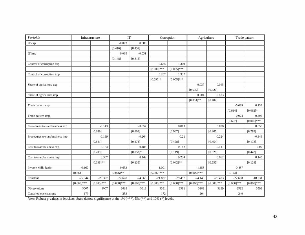
Variable Infrastructure IT Corruption Agriculture Trade pattern IT exp -0.073 0.086
[ 0.416] 0.459][
IT imp 0.065 -0.031
[ 0.148] 0.812][
Control of corruption exp 0.685 1.309
[0.000]*** [0.005]***
Control of corruption imp 0.287 1.337
[0.092]* [0.005]***
Share of agriculture exp -0.037 0.045
[ 0.630] 0.820][
Share of agriculture imp 0.204 0.183
[0.0 14] 0.482]** [
Trade pattern exp -0.029 0.139
[ 0.614] .062]*[0
Trade pattern imp 0.024 0.303
[0.607] [0.005]***
Procedures to start business exp -0.143 -0.057 0.013 0.038 0.058
[0.689] [0.803] [0.967] [0.905] [0.789]
Procedures to start business imp -0.199 -0.264 -0.21 -0.224 -0.348
[0.641] [0.174] [0.428] [0.454] [0.173]
Cost to start business exp 0.154 0.188 0.182 0.111 0.07
[0.209] [0.052]* [0.119] [0.328] [0.442]
Cost to start business imp 0.307 0.142 0.234 0.062 0.145
[0.038]** [0.135] [0.042]** [0.555] [0.124]
Inverse Mills Ratio -0.162 -0.633 -1.091 -1.158 -0.487
[0.664] [0.026]** [0.007]*** [0.000]*** [0.123]
Constant -25.944 -20.397 -22.678 -24.965 -21.837 -29.457 -24.146 -25.433 -22.608 -18.331
[0.000]*** [0.005]*** [0.000]*** [0.000]*** [0.000]*** [0.000]*** [0.000]*** [0.000]*** [0.000]*** [0.000]***
Observations 3007 3007 3618 3618 3381 3381 3189 3189 3592 3592
Censored observations 179 253 172 204 240
Note: Robust p-values in brackets. Stars denote significance at the 1% (***), 5% (**) and 10% (*) levels.
42


