Trade Effects of the New Silk Road -...

Policy Research Working Paper 8694

Trade Effects of the New Silk Road

A Gravity Analysis

Suprabha BaniyaNadia RochaMichele Ruta

Macroeconomics, Trade and Investment Global Practice January 2019

Pub

lic D

iscl

osur

e A

utho

rized

Pub

lic D

iscl

osur

e A

utho

rized

Pub

lic D

iscl

osur

e A

utho

rized

Pub

lic D

iscl

osur

e A

utho

rized

Produced by the Research Support Team

Abstract

The Policy Research Working Paper Series disseminates the findings of work in progress to encourage the exchange of ideas about development issues. An objective of the series is to get the findings out quickly, even if the presentations are less than fully polished. The papers carry the names of the authors and should be cited accordingly. The findings, interpretations, and conclusions expressed in this paper are entirely those of the authors. They do not necessarily represent the views of the International Bank for Reconstruction and Development/World Bank and its affiliated organizations, or those of the Executive Directors of the World Bank or the governments they represent.

Policy Research Working Paper 8694

This paper takes a first look at the trade effects of China’s Belt and Road Initiative, also referred to as the New Silk Road, on the 71 countries potentially involved. The initia-tive consists of several infrastructure investment projects to improve the land and maritime transportation in the Belt and Road Initiative region. The analysis first uses geo-ref-erenced data and geographical information system analysis to compute the bilateral time to trade before and after the Belt and Road Initiative. Then, it estimates the effect of improvement in bilateral time to trade on bilateral export values and trade patterns, using a gravity model and a com-parative advantage model. Finally, the analysis combines the

estimates from the regression analysis with the results of the geographical information system analysis to quantify the potential trade effects of the Belt and Road Initiative. The paper finds that (i) the Belt and Road Initiative increases trade flows among participating countries by up to 4.1 percent; (ii) these effects would be three times as large on average if trade reforms complemented the upgrading in transport infrastructure; and (iii) products that use time sensitive inputs and countries that are highly exposed to the new infrastructure and integrated in global value chains have larger trade gains.

This paper is a product of the Macroeconomics, Trade and Investment Global Practice. It is part of a larger effort by the World Bank to provide open access to its research and make a contribution to development policy discussions around the world. Policy Research Working Papers are also posted on the Web at http://www.worldbank.org/research. The authors may be contacted at [email protected].

Trade Effects of the New Silk Road: A Gravity Analysis

Suprabha Baniya, Nadia Rocha, Michele Ruta1

Keywords: Belt and Road Initiative, Transport Infrastructure, GIS Analysis, Trade Flows, Time

Sensitivity, Input‐output Linkages

JEL Codes: F14, F15, R41

1 Suprabha Baniya, Clark University ([email protected]), Nadia Rocha, World Bank ([email protected]), Michele Ruta, World Bank ([email protected]). We would like to thank Alvaro Espitia for his excellent research assistantship during the project. We are also grateful to Caroline Freund, Francois de Soyres, Lionel Fontagne, Mauricio Mesquita Moreira, Alen Mulabdic, Siobhan Murray, and seminar participants at University of Bologna, GTAP conference, IADB, Rand Corporation, World Bank for helpful comments. The findings, interpretations, and conclusions expressed in this paper are entirely those of the authors. They do not necessarily represent the views of the International Bank for Reconstruction and Development/World Bank and its affiliated organizations, or those of the Executive Directors of the World Bank or the governments they represent.

2

1. Introduction

A stated goal of China’s Belt and Road initiative is to strengthen economic integration and policy

coordination in the broad Eurasia region. The initiative includes a series of transportation

infrastructure projects, which are proposed along two pillars: the Silk Road Economic Belt and

the 21st Century Maritime Silk Road. Specifically, the “Belt” links China to Central and South Asia

and onward to Europe, while the “Road” links China to the nations of Southeast Asia, the Gulf

countries, East and North Africa, and on to Europe. Six economic corridors have been identified:

(1) the China‐Mongolia‐Russia Economic Corridor; (2) the New Eurasian Land Bridge; (3) the

China–Central Asia–West Asia Economic Corridor; (4) the China–Indochina Peninsula Economic

Corridor; (5) the China‐Pakistan Economic Corridor, and (6) the Bangladesh‐China‐India‐

Myanmar Economic Corridor.

This paper offers a first assessment of the impact of the new and improved BRI transport

infrastructure on trade flows of BRI countries.2 Specifically, we examine the potential trade

effects of the BRI using a combination of geographic and econometric analysis. First, we assess

the impact of the BRI on trading times using a new database on transport projects linked to the

BRI (de Soyres et al., 2018; Reed and Trubetskoy, 2018). Georeferenced data and geographical

information systems (GIS) analysis are used to compute the bilateral trade time between capitals,

ports and major cities (>100K) in the Belt and Road countries before and after the proposed

interventions.3 Second, we use a gravity model (Head and Mayer, 2014) to estimate the total

effect of bilateral trade time on bilateral exports and a comparative advantage model à la Nunn

(2007) to estimate the impact of bilateral time to trade on the export pattern in time sensitive

products and in products that rely on time sensitive inputs.

To assess the trade impact of the BRI, the GIS analysis and econometric estimates are combined.

These results are also used to investigate whether there is complementarity between

infrastructure improvements and policy reforms that promote trade facilitation, market access

2 There is no official list of “BRI countries”. In this paper, we focus on a list of 71 economies, including China, that are geographically located along the “Belt” and the “Road” (see Table A. 1). 3 The list of proposed interventions can be found in de Soyres et al. (2018).

3

and further regional integration between BRI countries. Specifically, the paper provides a series

of simulations on how the potential impact of BRI could be boosted once BRI countries work

towards reducing time delays at the border, decrease tariffs or sign “deep” trade agreements,

i.e. agreements that go beyond tariff reductions. To test the complementarity between transport

infrastructure improvements and trade reforms, we augment the gravity model to introduce an

interaction term between our main variable of interest, bilateral trading times, and the average

applied tariffs between two countries at the sectoral level or the “depth” of bilateral trade

agreements signed between BRI countries.

An important issue in the estimation of the trade effects of transportation infrastructure is

endogeneity. The plan to invest in these infrastructure projects could be driven by China’s rising

trade prospects with BRI countries (Constantinescu and Ruta, 2018). We address the potential

endogeneity between infrastructure and trade in different ways. First, we eliminate nodal

countries and the extractive sector from the analysis. Intuitively, if the goal of the BRI is for China

to access larger markets or to secure energy supplies, an analysis focused on transit countries

and non‐energy sectors should mitigate endogeneity problems. Second, we use an Instrumental

Variable (IV) approach. Specifically, we employ the physical geography features of transit

countries along any trade route as instruments for the bilateral transport time between the

trading partners. Third, in the comparative advantage model, we estimate a difference‐in‐

difference estimation that allows us to introduce a richer set of fixed effects, including country‐

pair and country‐sector, to control for other sources of omitted variable biases.

The results from the econometric analysis confirm that there is a negative relationship between

trading times and trade: a one‐day reduction in trading times increases exports between BRI

economies by 5.2 percent on average. In addition, trading times are particularly important for

time sensitive products that are used as inputs in production processes, suggesting that

reductions in shipping times are key in the presence of global value chains. Last, we find that

reducing border delays, having better market access to countries and signing deeper trade

agreements would magnify the trade impact of a reduction of time to trade due to new and

improved transport infrastructure.

4

We combine the estimates from the regressions with the results of the GIS analysis to quantify

the potential trade effects of the BRI. An upper‐bound estimate is that total BRI trade increases

by 4.1 percent. This assumes that trade in all products can switch transportation modes relatively

easily to take advantage of the improved transport links. A lower‐bound estimate, which assumes

that products cannot switch transportation mode, is that trade increases by 2.5 percent. The

trade effects of the BRI present a large variation across individual countries and across sectors.

Largest improvements in trade are predicted for countries in Sub‐Saharan Africa, Central and

Western Asia and for products that use time sensitive inputs such as chemicals. Complementing

BRI infrastructure improvements with trade reforms such as deepening trade agreements or

better market access would boost trade by respectively, 7.9 and 12.9 percent.

While there is much debate surrounding the Belt and Road Initiative, little rigorous economic

analysis on its effects has been done so far. Exceptions include Villafuerte, Coron and Zhuang

(2016) and Zhai (2018), who use a Computable General Equilibrium (CGE) model to assess the

impact of the BRI on trade and economic growth.4 Differently from the CGE approach, our paper

builds on a number of recent econometric studies. First, there is a recent literature that aims at

assessing the impact that reduction in time to trade, due to trade facilitation reforms or

infrastructure improvements, has on trade flows (e.g. Djankov, Freund and Pham, 2010;

Hummels and Schaur, 2013; and Baniya, 2017). Second, several studies analyze the trade effects

of infrastructure projects (Donaldson, 2013; Duranton, Morrow and Turner, 2012; Alder, 2015).

Finally, a subset of this literature also relies on georeferenced data and GIS analysis to assess the

trade and spatial effects of transport infrastructure (e.g. Roberts, Deichmann, Fingleton and Shi,

2010; Roberts, Deichmann, Fingleton and Shi, 2010).

The rest of the paper is organized as follows. Section 2 presents the GIS analysis. The econometric

strategy and results are discussed in Section 3. Section 4 outlines the trade impact of the BRI.

Concluding remarks follow.

4 Related work by de Soyres et al., Mulabdic and Ruta (2018) and Maliszewska and van der Mensbrugghe (2018) uses the data on trade costs from de Soyres et al. (2018) in a structural and CGE trade model respectively.

5

2. Estimating trading times using network analysis

To estimate the shipping times between two BRI locations, we use georeferenced data combined

with GIS analysis on a country’s transport network.5 The main objective of the network analysis

is to quantify the connectivity between capitals, ports and major cities (>100K) of BRI countries

before and after various planned interventions (see Figure 1).6 Trading times are assessed with

the transport network in 2013 (i.e. before the official launch of BRI) for a set of 1,818 cities across

71 BRI economies listed in Appendix Table A. 1. This section reviews the main steps that are

performed to assess the time it takes to trade across countries before the Belt and Road

interventions (the assessment of the updated transport network on trade times is discussed in

Section 4). It also highlights the main statistics deriving from this exercise.

A network analysis provides a more accurate measure of the real time it takes to ship goods

across countries, as it takes into account factors such as the quality and quantity of infrastructure,

physical obstacles (rough terrain) or other barriers (border and other delays). It also provides a

more realistic description of the travel routes of goods that are shipped between cities compared

to other measures such as the distance between capitals or main cities that are commonly used

in the trade literature.

5 The details of the methodology and data are discussed in de Soyres et al. (2018). 6 The list of interventions under the BRI has been identified in Reed and Trubetskoy (2018).

6

Figure 1: BRI transport projects

Source: Reed and Trubetskoy (2018)

A network solution involves finding the shortest path between two locations, where the length

of a path is the sum of a cumulative variable such as travel time (hours). Routing is determined

by minimum time cost path, where travel time is a function of physical distance, geographical

characteristics, speed and mode of transportation. In the baseline scenario, existing rail speed

(50 kph) and sea routes (25 kph) are assumed along the network. Other variables such as the

number of borders crossed along the route or how long it takes to load or unload the

merchandise at the port can also affect trading times and therefore can change the shortest path

connecting two locations. To account for this, information on border and port delays is included

in the GIS analysis. The total time spent at the border that is assigned to each pair of countries is

based on the importing and exporting trading times information from the Doing Business data

7

set. Estimates on the time it takes to load and unload the goods at the ports is taken from Slack

e al. (2018).

Before transportation infrastructure projects are implemented, bilateral trading times between

BRI economies are on average 383.1 hours, equivalent to 16 days, and they range between a

minimum of 0.9 hours to a maximum of 40.6 days (see Table 1). To perform the econometric

analysis on the impact of trading times on bilateral trade flows, the minimum time it takes to

connect cities is aggregated at the country pair level. To control for the fact that the economic

activity varies across cities, we compute a population weighted average of the shipping times

between each pair of cities that are in a pair of countries.

Table 1: Summary statistics of bilateral shipping times pre‐BRI

Obs. Mean Std. Dev. Min Max

Travel Time (hours) 4,891 383.112 192.625 0.89 974.781

At the regional level, before BRI transport projects, the East Asia & Pacific region has the highest

trading times vis‐a‐vis all the other regions, particularly with countries in Central & Eastern

Europe and Central & Western Asia (see Table 2). For example, it takes on average more than 30

days to ship goods between China and countries in Central & Eastern Europe such as Estonia,

Poland and Croatia. Shipping times between China and Central Asian countries such as Georgia

and Armenia are also high, amounting to 32.3 and 32.1 days on average. 7

Table 2: Average pre‐BRI trading times between regions

Avg. Travel time (days) CEE CWA EAS MEA SAS SSF

Central and Eastern Europe 3.6

Central and Western Asia 13.1 10.8

East Asia & Pacific 25.9 23.4 8.1

Middle East & North Africa 13.1 14.2 20.7 8.9

South Asia 22.3 19.6 16.2 14.9 11.8

Sub‐Saharan Africa 19.6 22.3 21.4 14.3 17.6 4.0

Regional 13.9 16.1 19.7 14.1 17.8 18.5

Note: Averaged over all country‐pairs in each region‐pair

7 Table A. 8 presents simple average trading times for all countries.

8

3. The impact of trading times on trade

i. Methodology

In this section, we build on the literature on trade times and trade discussed in the Introduction

and investigate how time to trade affects trade values between BRI economies. Intuitively, longer

time delays act as a tax on exports, especially in the context of global value chains, where goods

need to be shipped on time in order to ensure that production processes are not disrupted.

We begin by estimating the following augmented gravity equation:

𝑋 exp 𝛽 𝛽 𝐺𝑖𝑠𝑇𝑖𝑚𝑒 𝛽 𝑇𝑎𝑟𝑖𝑓𝑓 𝛽 𝑃𝑇𝐴 𝑑𝑒𝑝𝑡ℎ 𝐺𝑟𝑎𝑣𝑖𝑡𝑦 𝜆 𝛾

𝜀 , (1)

where the i,j and g subscripts correspond to the exporter, the importer and the hs6 product,

respectively; the dependent variable 𝑋 represents bilateral exports of product g from country

i to country j; 𝐺𝑖𝑠𝑇𝑖𝑚𝑒 represents our variable of interest and is calculated as the minimum

time it takes to transport a good from country i to country j in the baseline scenario presented in

Section 2. 𝐺𝑟𝑎𝑣𝑖𝑡𝑦 includes a set of gravity‐type variables associated with the exporter and the

importer such as sharing the same official language or border or past colonial relationship and

the strength of market penetration; 𝑃𝑇𝐴 𝑑𝑒𝑝𝑡ℎ captures the level of depth of preferential

trade agreements between the exporter and importer and is measured as the number of legally

enforceable8 disciplines that are included in a PTA. 𝑇𝑎𝑟𝑖𝑓𝑓 refers to the logarithm of the

average tariff applied by country j to country i for hs4‐level product k plus one. Finally, we include

exporter‐product (𝜆 and importer‐product (𝛾 fixed effects to control for factors such as

comparative advantage, foreign industrial demand for intermediate inputs that can increase the

exports, availability of intermediate inputs in the local economy that can raise the industrial

8 The legal enforceability of the PTA disciplines is established according to the language used in the text of the agreements. In other words, it is assumed that commitments expressed with a clear, specific and imperative legal language can more successfully be invoked by a complainant in a dispute settlement proceeding and therefore are more likely to be legally enforceable. In contrast, unclear legal language might be related to policy areas that are covered but that might not be legally enforceable. See Hofmann, Osnago and Ruta (2017).

9

expenditure on inputs and thereby raise the production and exports, market potential, trade

intensity, and agglomeration forces or co‐location effects (see Hummels and Hillberry, 2002).

The data for the main variable of interest (𝐺𝑖𝑠𝑇𝑖𝑚𝑒 ) were described in detail in the previous

section. Other variables that are used in the econometric analysis come from usual sources.

Export flows are collected from Comtrade at the hs6 level for the year 2013. Information on the

gravity variables (common language or border or past colonial relationship and the strength of

market penetration) comes from BACI data set produced at Center for Prospective Studies and

International Information. Product‐level information on preferential and Most Favored Nation

tariffs imposed by countries comes from the new ITC‐World Bank data set on preferential tariffs

(Espitia et al, 2018). Data on the depth of preferential trade agreements come from the new

World Bank database on the content of preferential trade agreements (Hofmann, Osnago and

Ruta, 2017). Table A. 2 in the appendix presents the correlation between all the variables that

are used in the estimations.

ii. Results

Table 3 presents the results of the estimation of equation 1 for a set of 71 countries and 5,039

HS‐6 products in 2013. Regressions are estimated both using a linear model (OLS) and a Poisson

pseudo maximum likelihood model (PPML) to control for the presence of zero trade flows. The

results confirm a negative relationship between trading time and exports. The coefficient of the

𝐺𝑖𝑠𝑇𝑖𝑚𝑒 variable represents the percentage change in exports to a one hour increase in trading

times. Results from the PPML model suggest that a one‐day increase in trading times decreases

exports by 5.2 (0.00217*100*24hrs) percent on average. Our results are in line with what has

been found in the literature on the impact of trading times on exports. Papers such as Djankov,

Freund and Pham (2010) find that, on average, each additional day that a product is delayed prior

to being shipped reduces trade by at least 1 percent. They also find that the impact of delays is

significantly higher for developing countries. Other papers focusing on the Sub‐Saharan Africa

region find that a one‐day reduction in inland travel times leads to a 7 percent increase in exports

(Freund and Rocha, 2011).

10

Table 3: Effects of Time to Trade on Trade Values

OLS PPML

(1) (2)

GIS Time ‐0.00233*** ‐0.00217***

(0.000187) (0.000153)

Ln(tariff+1) ‐1.315*** ‐1.871***

(0.376) (0.285)

PTA Depth 0.0208*** 0.0195***

(0.00290) (0.00211)

Observations 1,205,865 8,287,250

R‐squared 0.619 0.499

Note: Standard errors in parentheses are clustered by exporter‐importer pair. *** p<0.01, ** p<0.05, * p<0.1

The coefficient of our control variable, PTA depth, suggests that BRI countries with deeper

agreements trade more on average. Specifically, having one extra provision included in the

agreement increases trade by 1.9 percent on average. This result is in line with the literature on

the trade effects of deep trade agreements.9 In terms of tariffs, a 1 percent increase in tariff rates

will reduce exports by 1.8 percent on average. Other standard gravity variables (not reported)

have the usual signs found in the literature.

Different products are likely to respond differently to changes in trade time because time

sensitivity varies by product. To take a first look into the potential heterogeneity that the variable

trading times can have on exports at the product level, we run equation (1) for each hs4 product10

‐‐we come back to this issue in Section 3.iv using a different specification based on Nunn (2007).

Specifically, we estimate the following equation:

𝑋 exp 𝛽 𝛽 𝐺𝑖𝑠𝑇𝑖𝑚𝑒 𝛽 𝑇𝑎𝑟𝑖𝑓𝑓 𝛽 𝑃𝑇𝐴 𝑑𝑒𝑝𝑡ℎ 𝐺𝑟𝑎𝑣𝑖𝑡𝑦 𝜆 𝛾 𝜀

9 Papers such as Orefice and Rocha (2014) find that deeper agreements increase trade across countries by 2 percent on average. More recent research by Mattoo, Mulabdic and Ruta (2017) finds that trade between country pairs that sign an agreement with the highest depth increases by around 12.5 percent. 10 Regressions cannot be run at the hs6 level as some of the products have very few observations and the PPML does not always converge.

11

Notice that now the fixed effects that are included in the regression are at the country level

instead of country‐product level.

Results for the product‐level estimations aggregated at the sectoral level are presented in Table

4. The negative impact of time delays on exports ranges between ‐0.002 and ‐0.06. For sectors

such as wood/wood products (e.g. chemical wood pulp and wood wool) and vegetable products

(e.g. ground nut oil and its fractions, mate, and cucumbers and gherkins), the GIS time coefficient

is the highest, suggesting that these sectors are more sensitive to time variations. Specifically, a

one‐day increase in export delays decreases exports in these industries by more than 25 percent

on average. For other sectors such as footwear/headwear, miscellaneous products (works of art

and clocks/watches) and transportation equipment, the impact of a one‐day increase on exports

is much lower and equal to 3.9 percent on average.

Table 4: Average effect of GIS Time to trade – At the 4‐digit level aggregated by sector

Sector Coefficient

Wood & Wood Products ‐0.058

Vegetable Products ‐0.051

Stone / Glass ‐0.011

Mineral Products ‐0.010

Raw Hides, Skins, Leather, & Furs ‐0.007

Animal & Animal Products ‐0.005

Foodstuffs ‐0.003

Plastics / Rubbers ‐0.003

Chemicals & Allied Industries ‐0.003

Metals ‐0.003

Textiles ‐0.003

Machinery / Electrical ‐0.003

Transportation equipment ‐0.003

Miscellaneous (Hs 90‐97) ‐0.002

Footwear / Headgear ‐0.002

12

iii. Robustness checks

The previous results might be subject to endogeneity deriving from omitted variables bias and

reverse causality. Omitted variables bias arises when there are unobserved country‐pair specific

policy variables (peaceful relationship, common legal origin, etc.) that affect both exports and

trading times. The rich set of fixed effects that are included in the regressions together with the

policy controls that vary at the country‐pair level control for a significant degree of the omitted

variables. Moreover, in a second exercise that is presented in sub‐section (iv), we estimate the

impact of trading times on exports of time sensitive products using a difference in difference

approach. In this case, the higher number of fixed effects that are included in the regression

allows us to fully control for omitted variables (see section‐below).

Reverse causality may arise when the time to export variables are likely to be correlated with

country exports. An improvement of rail or ports infrastructure and administrative time costs has

positive effects on exports. However, trade partners that have better trade prospects or that

wish to improve their current trade volume will also invest more on such trade facilitating

infrastructure. Such incentives of infrastructure reform are clearly important in the case of the

Belt and Road Initiative. In particular, the rising trade prospects of China and its increasing need

for energy supplies are some of the major incentives to improve infrastructure in the context of

the BRI. To control for reverse causality, we use three types of robustness checks. First, we

estimate the regressions excluding the nodal countries in the BRI, mainly Europe and China,

which are those that are trading more between them. Second, we re‐estimate the regressions

excluding the extractive industries. Third, we follow an instrumental variable approach to

estimate equation (1).

For the instrumental variables estimation, we follow the literature and instrument travel times

between trading partners using the mean physical geography features of transit countries along

any trade route.11 The set of geographical variables that are used to compute the instruments

are taken from Nunn and Puga (2009) and include the percentage of moderately to highly rugged

11 Geographical characteristics of a country have been used in the past by papers such as Limao and Venables (2001) to instrument for transport infrastructure.

13

land area and the proximity to the coast (percentage of land area within 100km of the nearest

ice‐free coastline). These geographical features are clearly exogenous to trade as countries are

naturally endowed with them. In addition, they have a direct impact on the ability of bilateral

trade partners to transport goods on time. Trade routes that are highly rugged (presence of rough

and uneven land surfaces) tend to have lower quality of land transportation infrastructure, while

trade routes that are closer to the coast tend to have well established maritime ports and

transport infrastructure.

Results from the first stage regression (see appendix

14

Table A. 3 and Table A. 4) confirm that the proposed instruments are a good predictor of

transport infrastructure. Trading routes that are less rugged and near to the coast have lower

bilateral time to trade. The F‐statistics reported in

15

Table A. 3 and Table A. 4 also confirm that the instruments are not weak. In addition, the low

correlations between export values and geographical features (see Table A. 5) support the fact

that they meet the exclusion restriction criteria.

To control for the potential reverse causality of other explanatory variables such as the depth of

preferential trade agreements, we instrument PTA depth between country i and country j with

the trade weighted average depth of all the agreements signed by i and j with third countries.

This type of instrumental variable approach has already been used in the literature (see, for

instance, Orefice and Rocha, 2014 and Laget et al., 2018). We aggregate tariffs at the HS4 level,

so the degree of endogeneity between trade and tariffs at the product level decreases.12

Table 5 presents the results of the impact of trading times on export values once we control for

endogeneity. Estimations excluding nodal countries and products from the extractive industries

are very similar to those in the baseline regression and suggest that a one‐day decrease in trading

times increases trade by 5.2‐6.6 percent on average (columns 1, 2, 4 and 5). The second‐stage

results of the instrumental variable regressions are presented in column (3). The magnitude of

the coefficients on trading times is larger compared to those in the baseline results and show

that a one‐day decrease in trading times increases exports by 12 percent on average. One

potential reason for this is that the variable, GIS time, might be subject to measurement error as

it might not fully reflect the role of geography in explaining the connectivity between countries.

Table 5: Sorting out endogeneity

OLS PPML

Eliminate CHN‐EU

Eliminate Extraction

IV Eliminate CHN‐EU

Eliminate Extraction

(1) (2) (3) (4) (5)

GIS Time ‐0.00264*** ‐0.00233*** ‐0.00499*** ‐0.00273*** ‐0.00215***

(0.000198) (0.000188) (0.000995) (0.000166) (0.000153)

Ln(PRF+1) ‐1.166*** ‐1.314*** 1.401 ‐1.686*** ‐1.889***

(0.367) (0.377) (0.974) (0.276) (0.285)

PTA Depth 0.0228*** 0.0208*** 0.00803 0.0226*** 0.0194***

12 As an extra check, regressions are conducted aggregating tariffs at the hs2 level. Results presented in appendix Table A. 6 are very similar to those in the baseline regression.

16

(0.00293) (0.00291) (0.0137) (0.00199) (0.00211)

Observations 1,140,459 1,192,038 1,224,775 8,093,490 8,135,016

R‐squared 0.622 0.617 0.603 0.511 0.500


Two additional robustness tests are performed. First, to control for year‐specific effects in our

analysis, regressions are estimated using export values in periods t‐1 and t+1, where t equals

2013. Results presented in appendix Table A. 7 are in line with the baseline results and confirm

the negative impact of trading times on export values. Second, we also conduct regressions

excluding the trade flows of the exporting country from the computation of the importer market

sizes to avoid endogeneity. Results are once again in line with those in our baseline specification

(see columns 3 and 6 of Table A. 7 in the appendix).

iv. Time sensitivity and export delays

As discussed in Section 3.i, time delays should have a greater effect on export patterns of time

sensitive goods. In this section, we go one step further and examine how the ability of bilateral

trade partners to transport goods on time determines their comparative advantage in products

that are time sensitive (direct time sensitivity) and that value timely delivery of their inputs

(indirect time sensitivity).

Following Nunn (2007), we adopt an empirical specification that explains export values by the

interactions of exporter‐importer specific characteristics with product specific characteristics. In

particular, we estimate the following specification:

lnX β β lnGisTime *t β lnGisTime *t̃ Controls μ π η ρ λ

γ ε (2)

where 𝛽 ∗ 𝑡 represents the direct effect of transportation infrastructure projects, while 𝛽 ∗ �̃�

represents the indirect effect of transportation infrastructure projects arising through the input‐

output linkages. Specifically, the direct effect comes from the improvement in the ability to

transport the final products to the consumers or end users on time, whereas, the indirect effect

comes from the improvement in the ability to access the intermediate inputs on time. Hence, a

17

one‐day decrease in bilateral time to trade leads to an increase in the bilateral export pattern by:

𝛽 ∗ 𝑡 𝛽 ∗ �̃� %.

The results presented in Table 6 show that the impact of trading times is relatively higher for

products that are time sensitive to their consumers or end users and that use time sensitive

inputs in production. In addition, the indirect effect (impact of trading times on products that

highly use time sensitive inputs in production) is higher than the direct effect (impact of trading

times on products that are time sensitive to their consumers), suggesting that improving trading

times is particularly important in a world of global value chains, where time sensitive inputs are

imported for production.

To gauge the magnitude of the estimates on the interaction between time reductions and direct

time sensitiveness, we evaluate the coefficients for two sets of industries: textiles, leather and

apparel, and motor, parts and transport equipment. These industries fall respectively in the 25th

and 75th percentile of the direct time sensitivity distribution. The increase in average trade from

a one‐day reduction in trading time is 0.17 percentage points higher for products within the

motor, parts and equipment sector compared to products in the textile, leather and apparel

industries. Conversely, the impact of reduction in timeliness on exports of products that use time

sensitive inputs is 0.23 percentage points higher for products in the paper and metals industries,

which fall in the 75th percentile of the indirect time sensitivity distribution, compared to products

in the textiles, leather and apparel industries, which are in the 25th percentile of the distribution.

Table 6: Time sensitive products and products using time sensitive inputs

OLS PPML

(1) (2)

GIS Time * t0 (Direct Effect) ‐0.00925*** ‐0.00886***

(0.00105) (0.000701)

GIS Time * t1 (Indirect Effect) ‐0.0261*** ‐0.0388***

(0.00333) (0.00181)

Ln(PRF+1) ‐0.509*** ‐0.220**

(0.151) (0.0910)

18

Observations 1,235,877 8,308,722

R‐squared 0.669 0.627


v. Complementarity between infrastructure improvements and trade reforms

In this sub‐section, we assess the complementarity of trade policy reforms (deepening trade

agreements and improving market access) on the one hand and infrastructure improvements in

the BRI region on the other hand. To do this, we introduce an interaction term between the GIS

variable of shipment times across countries and the policy variable (𝑃𝑜𝑙𝑖𝑐𝑦 ), capturing

respectively, the level of depth of agreements signed between a pair of countries ij or the average

preferential tariffs that the importer j is imposing to i in sector k:

𝑋 exp 𝛽 𝛽 𝐺𝑖𝑠𝑇𝑖𝑚𝑒 𝛽 𝑇𝑎𝑟𝑖𝑓𝑓 𝛽 𝑃𝑇𝐴𝑑𝑒𝑝𝑡ℎ 𝛽 𝑃𝑜𝑙𝑖𝑐𝑦 ∗ 𝐺𝑖𝑠𝑇𝑖𝑚𝑒 𝐺𝑟𝑎𝑣𝑖𝑡𝑦 𝜆 𝛾 𝜀 (3)

The results presented in Table 7 highlight the complementarity between infrastructure

improvements and trade reforms.13 The positive impact of a reduction in trading times is

magnified for country‐pairs that are involved in deeper trade agreements (e.g. countries that

have better institutions and that share a common regulatory framework in trade related

disciplines such as investment, intellectual property rights, competition policy and technical

barriers to trade among others) as opposed to country pairs that have shallow agreements (see

columns 1 and 2). Specifically, the positive impact of a one‐day reduction in trading times is 1.1

percent higher (6.3 percent) for country‐pairs that are part of the European Union, the deepest

agreement in the BRI sample of countries, compared to countries that are part of very shallow

agreements (agreements including only one provision).

In terms of market access, the positive impact of reducing trading times is dampened for country‐

pair‐products with lower levels of tariff liberalization (see columns 3 and 4). Whereas a one‐day

reduction in trading times without reductions in tariff rates will increase average exports of

13 The IV regressions are excluded from this exercise given the complexity to instrument and interpret the interaction between endogenous variables.

19

country‐pair‐products by 6.3 percent on average, exports of products subject to 1 and 10 percent

reductions in tariff rates will increase by 6.6 and 8.9 percent on average respectively as a result

of a one‐day reduction in trading times. A one‐day reduction in trading times with a half‐

reduction or full reduction of tariff rates (tariff rate=0) will boost exports by respectively 19.5 and

32.7 percent on average.

Table 7: Complementarity between infrastructure improvements and trade reforms

Deepening trade agreements Improving market access

OLS PPML OLS PPML

(1) (2) (3) (4)

GIS Time ‐0.00228*** ‐0.00214*** ‐0.00271*** ‐0.00262***

(0.000185) (0.000149) (0.000190) (0.000159)

PTA Depth 0.0287*** 0.0277*** 0.0190*** 0.0168***

(0.00329) (0.00253) (0.00291) (0.00213)

PTA Depth * GIS Time ‐0.000105*** ‐0.000111***

(2.30e‐05) (2.18e‐05)

Ln(PRF+1) ‐1.728*** ‐2.284*** ‐3.849*** ‐5.254***

(0.360) (0.278) (0.644) (0.547)

Ln(PRF+1) * GIS Time 0.00713*** 0.00883***

(0.00134) (0.00108)

Observations 1,205,865 8,287,250 1,205,865 8,287,250

R‐squared 0.620 0.501 0.619 0.502


4. Assessing the potential impact of BRI on trade

In this section we assess the potential impact of BRI improvement on export flows. First, we study

the time improvements that derive from BRI transportation projects using GIS analysis and then

we focus on trade effects. The following cases are presented: improvements in infrastructure

only, improvements in both infrastructure and border delays and improvements in infrastructure

along economic corridors. We also assess the overall effect of BRI transportation projects in the

presence of deeper agreements and when better market access is granted to countries.

20

i. Effects of BRI transportation projects on trade times

To assess improvements in trading times after BRI projects are implemented, a higher speed is

assumed for the parts of the new or improved existing network. The baseline scenario discussed

in Section 2 uses existing rail speed (50 kph) and sea routes (25 kph), while the post‐BRI scenario

includes proposed new rail links and main rail along the route segments that have been improved

at the increased speed (75 kph). To capture the upgrading of existing ports, it is assumed that the

time it takes to handle the merchandise in the port decreases to the minimum time estimates in

the region that are provided in Slack et al. (2018).

The choice of a shipping route between two locations can depend on factors other than time

(and distance), such as the monetary cost determined by the mode of transportation (railway or

maritime). To take into account the trade‐off between shorter trade/travel times of railway

connectivity and cheaper monetary costs associated with maritime travel, two extreme

scenarios are created post‐BRI. In the first scenario (referred to as the lower bound scenario), a

high preference for using maritime links whenever available is assumed. Here the improvements

in shipping times will derive either from improvements in existing ports or from alternative

maritime routes where new land connectivity with certain cities exists. In the second scenario,

the upper bound scenario, the preference for maritime transport is removed, implicitly allowing

for modal substitution between maritime and railway transport whenever the time/distance is

lower transporting goods by land.

Table 8 shows that the Belt and Road Initiative would both create new land and maritime

connections among BRI economies and reduce trade times by 2.8 percent on average, equivalent

to 11.7 hours (0.5 days), assuming that there is a preference for maritime transport after BRI

interventions (lower‐bound scenario). For the upper‐bound scenario, where change in mode of

transportation from sea to rail is allowed, the average reduction in trading times is 4.4 percent,

equivalent to 17.6 hours (0.7 days). Changes in trade time vary widely, with reductions that range

between zero and 9.6 days.

Table 8: Trade time improvements post‐BRI

Lower‐bound Obs. Mean Std. Dev. Min Max

21

Change in travel time (hours) 4,891 ‐11.6911 19.4378 ‐220.8858 0

Change in travel time (%) 4,891 2.8393 5.2048 0 86.9523

Upper‐bound

Change in travel time (hours) 4,891 ‐17.6081 25.1575 ‐231.5271 0

Change in travel time (%) 4,891 4.3604 6.1668 0 86.9523

Average trade time reductions across pairs of regions range between 0.4 and 19.4 percent in the

lower bound scenario and between 0.8 and 20.8 percent in the upper bound scenario (Table 9).

Largest reductions in time to trade are predicted for country‐pairs within Central & Western Asia

(19.4 in the lower bound and 20.8 in the upper bound). Across regions, the highest time

decreases take place between Sub‐Saharan Africa and East Asia & Pacific in the lower bound (7.8

percent); and between Central & Western Asia and East Asia & Pacific in the upper bound (9.1

percent). 14

Table 9: Average change in time to trade (%) between regions

a. Lower‐bound b. Upper‐bound

Note: Averaged over all country‐pairs in each region‐pair

ii. Effects of BRI transportation projects on trade

To estimate the impact of BRI on trade, we multiply the trade elasticities of time obtained from

the gravity estimation and the time reductions derived from GIS analysis: ∆𝑙𝑛𝑋 100 ∗ 𝛽 ∗

14 Time reductions for the lower and upper bound scenarios at the country level are presented in Appendix Table A. 8.

22

∆𝐺𝑖𝑠𝑇𝑖𝑚𝑒 at the product level. We then calculate the total pre‐BRI and post‐BRI trade for each

country‐pair. An upper‐bound estimate of the overall effect of the BRI suggests that total trade

within BRI countries increases by 4.1 percent. This assumes that trade in all products can switch

transportation modes relatively easily to take advantage of the improved transport links. A lower‐

bound estimate, which assumes that products cannot switch transportation mode, is that total

trade within BRI countries increases by 2.5 percent.

The discussion below highlights the heterogeneity of the trade effects of the BRI across regions,

countries and sectors. Table 10 shows the results on the impact of BRI improvements on trade

between BRI regions for the lower and upper bound scenarios respectively. Trade gains range

between 1.5 and 5.5 percent in the lower bound scenario and between 2.3 and 8.6 percent in

the upper bound scenario with East Asia & Pacific and Sub‐Saharan Africa experiencing the largest

increments in exports (5.5 and 5.1 percent, respectively in the lower bound scenario and 8.5 and

8.6 percent in the upper bound scenario). Across pairs of regions, some interesting patterns

appear. In the lower‐bound scenario, the highest changes in trade occur between East Asia &

Pacific and Sub‐Saharan Africa. In the upper bound scenario, exports from Sub‐Saharan Africa to

Central & Western Asia increase the most. This is consistent with the fact that the upper bound

scenario allows for a greater flexibility in changing transport mode from maritime to rail.

Table 10: Change in total trade (%) between regions


Note: Change in trade is calculated as the difference between pre‐BRI and post‐BRI trade for each country ‐pair in each region‐pair

At the country level, expected trade gains from BRI reflect both the extent of improved

connectivity and the export structure of the country. Figure 2 plots the expected change in

23

exports for the BRI countries against their levels of trade pre‐BRI. Countries such as Uzbekistan,

the Islamic Republic of Iran, Oman, Maldives and Myanmar benefit the most after improvements

in trading times, with an increase in their exports above 7 percent. Other countries, such as China

,and Saudi Arabia, will benefit the most in terms of value of their exports given their already high

trade within the BRI. While in some cases trade gains are sizeable, an important constraint to

trade expansion is the persistence of significant policy barriers for many BRI countries. We

expand on this in the next sections.

At the sectoral level, the positive impact of the BRI ranges between 3.5 and 84 percent. Industries

gaining the most from the BRI include wood/wood products (e.g. chemical wood pulp and wood

wool) and vegetable products (e.g. ground nut oil and its fractions, mate, and cucumbers and

gherkins). Their exports will increase by more than 60 percent. In contrast, exports of industries

such as miscellaneous products (works of art and clocks/watches), metals and machinery will

increase by 5 percent or less after the BRI (see Figure 3). The effects of BRI transportation projects

on the exports of different sectors depend on their time sensitivity ‐direct and indirect. Figure 4

shows that reduction in trade times will increase specialization in sectors such as livestock,

vegetable, fruits, nuts and crops, which will benefit the most from the improvement in the ability

to transport the final products on time to the consumers or end users (direct effect).

Specialization in exports from meat products, chemicals, ferrous metals, rubber and plastics will

also increase given the improvement in the ability to access the intermediate inputs on time

(indirect effect).

24

Figure 2: Change in total exports by country

Note: Change in trade is calculated as the difference between pre‐BRI and post‐BRI trade for each country

Figure 3: Change in total exports by sector

Note: Change in trade is calculated as the difference between pre‐BRI and post‐BRI trade for each sector

KEN TZA

CHN

MMR

THA

KGZ

TKM

UZB

IRQ IRNKWT OMNQAT

SAU

YEM

MDV

10

12

14

16

18

20

Log

(Pre

-BR

I exp

orts

)

0 5 10 15Percentage change in Trade

East Asia & Pacific Europe & Central Asia Miidel East & North Africa

South Asia Sub-Saharan Africa

Animal & Animal Products

Mineral Products

Chemicals & Allied Industries

Plastics / Rubbers

Raw Hides, Skins, Leather, & Furs

Footwear / Headgear

Stone / Glass

Machinery / Electrical

Transportation

Vegetable Products

Foodstuffs Wood & Wood Products

Textiles

Miscellaneous

Metals

16

17

18

19

20

21

Log

(Pre

-BR

I exp

orts

)

0 20 40 60 80Percentage change in Trade

25

Figure 4: Effects of BRI on the trade pattern (% Change)

Note: (i) The impact is estimated using the sector specific average time sensitivity characteristics irrespective of the regional production

and trade structure. (ii) Impact is calculated using ∆𝑙𝑛𝑋 100 ∗ 𝛽 𝑡 𝛽 �̃� ∗ ∆𝐺𝑖𝑠𝑇𝑖𝑚𝑒 with the average change in time to

trade from the upper‐bound scenario (17.61 hours)

iii. Complementarity between improved infrastructure, corridor management and trade

facilitation reform

In this section, we study two alternative cases for reductions in trading times after BRI are

presented: (i) improvements in infrastructure combined with reductions in border delays, and (ii)

improvements in infrastructure along economic corridors. In the first case, time improvements

after BRI are computed in the GIS analysis assuming that border delays are reduced 50 percent

across countries. In the second case, we assume that improvements in corridor management and

decreases in congestion take place after BRI interventions along the corridors. To take this into

account, we assume that improvements in the rail links after the BRI intervention apply along the

economic corridors (for the whole rail instead of the segment that is new or improved).

0.0 0.2 0.4 0.6 0.8 1.0 1.2

Chemical, ferrous metals, rubber, plastics

Extraction

Grains, Seeds and Fibers

Livestock

Machinery, parts and electronics

Meat Products

Motor, parts and Transport

Other Mnfcs (paper, metals, mnfcs nec)

Processed food

Textile, Leather and Apparel

Vegetable, fruits, nuts, crops

Wood and mineral prods

Effects on the Trade Patttern

Direct effect Indirect effect

26

Reductions in total trading times for the upper bound scenario are on average 10.9 percent when

border delays are reduced and 4.8 percent in the presence of improved economic corridors

(Figure 5). Countries in regions such as Central & Western Asia, South Asia and Middle East &

North Africa would reduce their average trading times by more than 10 percent if border delays

are improved. Improvements in corridor management would significantly reduce trading times

in other regions such as East Asia & Pacific and Sub‐Saharan Africa.

Figure 5: Change in average time to trade (%) – Upper bound scenario

Note: Averaged over all country‐pairs for each country.

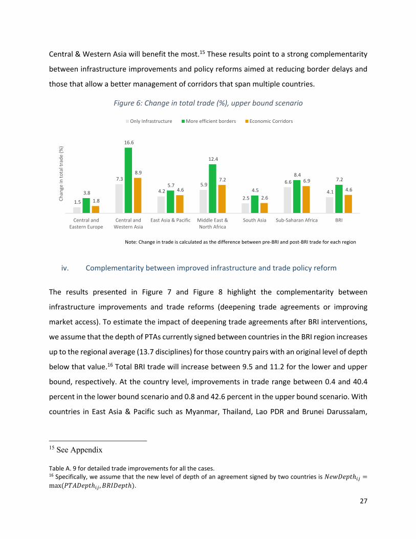
In terms of trade flows, the overall impact of the BRI on total exports ranges between 3.1 and 7.2

percent when border delays are reduced and between 2.6 and 4.6 percent in the presence of

improved economic corridors. Results at the regional level are illustrated for the upper bound

scenario in Figure 6. Improvements in infrastructure combined with reductions in border delays

will increase trade by more than 10 percent for regions such as Central & Western Asia and

Middle East & North Africa. In the same way, once the BRI intervention along the entire economic

corridors are implemented, countries from Sub‐Saharan Africa, Middle East & North Africa and

0

5

10

15

20

25

30

SYR

MNE

ALB BIH TLS

MKD

HRV

SVN

IRQ

CZE

MDA

EST

KWT

JOR

ROM

SGP

ARE

QAT

BGR

NPL

BHR

OMN

BTN

SAU

ARM

SRB

GRC

UKR

BGD

HUN

LKA

SVK

LAO

EGY

RUS

POL

IND

IDN

YEM

GEO LVA

PSE

BLR ISR

AFG TJK

LTU

BRN

IRN

PHL

LBN

TUR

TKM

TWN

TZA

PAK

MYS

DGI

KEN

CHN

AZE

MNG

MDV

MMR

VNM

KAZ

KHM

KGZ

THA

UZB

Chan

ge in

average tim

e to trade (%

)

Only Infrastructure More efficient borders Economic Corridors

27

Central & Western Asia will benefit the most.15 These results point to a strong complementarity

between infrastructure improvements and policy reforms aimed at reducing border delays and

those that allow a better management of corridors that span multiple countries.

Figure 6: Change in total trade (%), upper bound scenario

Note: Change in trade is calculated as the difference between pre‐BRI and post‐BRI trade for each region

iv. Complementarity between improved infrastructure and trade policy reform

The results presented in Figure 7 and Figure 8 highlight the complementarity between

infrastructure improvements and trade reforms (deepening trade agreements or improving

market access). To estimate the impact of deepening trade agreements after BRI interventions,

we assume that the depth of PTAs currently signed between countries in the BRI region increases

up to the regional average (13.7 disciplines) for those country pairs with an original level of depth

below that value.16 Total BRI trade will increase between 9.5 and 11.2 for the lower and upper

bound, respectively. At the country level, improvements in trade range between 0.4 and 40.4

percent in the lower bound scenario and 0.8 and 42.6 percent in the upper bound scenario. With

countries in East Asia & Pacific such as Myanmar, Thailand, Lao PDR and Brunei Darussalam,

15 See Appendix Table A. 9 for detailed trade improvements for all the cases. 16 Specifically, we assume that the new level of depth of an agreement signed by two countries is 𝑁𝑒𝑤𝐷𝑒𝑝𝑡ℎmax 𝑃𝑇𝐴𝐷𝑒𝑝𝑡ℎ , 𝐵𝑅𝐼𝐷𝑒𝑝𝑡ℎ .

1.5

7.3

4.2 5.9

2.5

6.6

4.1 3.8

16.6

5.7

12.4

4.5

8.4 7.2

1.8

8.9

4.6

7.2

2.6

6.9

4.6

Central andEastern Europe

Central andWestern Asia

East Asia & Pacific Middle East &North Africa

South Asia Sub‐Saharan Africa BRI

Chan

ge in

total trade (%

)

Only Infrastructure More efficient borders Economic Corridors

28

increasing their exports by more than 30 percent. Intuitively, deepening trade agreements would

allow BRI economies to reduce trade costs and discrimination associated to border and behind

the border policies, such as trade remedies (e.g. antidumping duties), competition and

investment policy.

Figure 7: Change in trade – Deepening trade agreements


Note: Change in trade is calculated as the difference between pre‐BRI and post‐BRI trade for each country

In terms of market access, we assume that as an incentive to promote trade along the route,

tariff rates among BRI countries are reduced by half. Specifically, tariff rates will decrease from

5.9 to 2.9 percent on average. The combination of lower tariffs and lower BRI trading times leads

to increases in trade among BRI economies between 10.9 and 12.9 percent for the lower and

upper bound scenarios, respectively. Results highlighting the average increase in trade by country

for the upper bound scenario are presented in figure 8. The positive impact of the BRI will be

boosted significantly for low and lower middle‐income countries, which currently face high levels

of protection. Specifically, their exports will increase by 38 and 19 percent on average,

respectively in the upper bound scenario.

29

Figure 8: Change in total trade – Improving market access (upper bound scenario)

Note: Change in trade is calculated as the difference between pre‐BRI and post‐BRI trade for each country.

5. Conclusion

This paper is a first attempt to examine the effects of the Belt and Road Initiative of China on

bilateral times to trade, and the resulting trade impacts for the Belt and Road countries using a

combination of geographic and economic analysis. We particularly focus our analysis on the land

and maritime transportation infrastructure reform that improve the connectivity of the 70

countries (plus China) that will potentially participate to the initiative. An important caveat is that

significant uncertainty attaches to our estimates: the BRI is a fluid project and the details of the

infrastructure investments are not known. Specifics on how the initiative will shape up will

obviously affect how it will impact shipment times, and ultimately, trade flows.

Keeping this caveat in mind, our results suggest that BRI transport projects would both create

new land and maritime connections in the broad Eurasia region and would reduce trade times

along the existing transport links between 2.8 percent (assuming that exporters do not switch

mode of transportation ‐lower bound) and 4.4 percent (assuming that exporters can switch

transport modes relatively easily ‐upper bound). When improvements in infrastructure are

combined with decreases in border delays, reductions in trading times are equal to 7.4 and 10.9

AFG

TZA

NPL

BTN GEO PHL

SYR LAO JOR

IDN

UKR

ARM EG

Y

MDA VNM

MMR

MNG KGZ D

JIKHM YE

M

IND PAK TJK

UZB

KEN

LKA

BGD

HRV

ROU

BIH BLR

BGR

AZE RUS

MYS

TKM

ALB KAZ IRQ LBN

MKD

CHN TH

ATU

R

IRN

MDV

SGP

TWN

SVN

HUN

BRN

CZE GRC

LVA

SVK

BHR

POL

EST LTU ISR

ARE

SAU QAT

KWT

OMN

0

10

20

30

40

50

60

70

Chan

ge in

trade (%

)

Low income Lower middle income Upper middle income High income

30

percent for the lower and upper bound scenarios respectively. These results suggest that the

positive impact of the BRI on trading times will be magnified if countries also implement trade

facilitation reforms.

We find that BRI infrastructure improvements could increase total trade among BRI economies

between 2.5 percent to 4.1 percent. Policy reforms aimed at reducing border delays and those

that allow a better management of corridors would complement BRI transportation projects.

Indeed, results show that BRI transportation projects increase total exports among BRI

economies by 4.6 percent in the presence of improved economic corridors and by 7.2 percent

when border delays are reduced. Finally, we find that deeper trade agreements and improved

market access would magnify the trade impact of BRI infrastructure projects, increasing total

exports by 11.2 and 12.9 percent, indicating that trade gains would be larger if trade cooperation

complemented infrastructure cooperation.

Differences in the BRI impact across countries reflect both the extent of improved connectivity,

and the export structure of the country—time‐sensitive products and products that require time‐

sensitive inputs are highly impacted. The biggest trade gains stem from improvements in trade

times for inputs whose timely delivery is highly valued by producers. Put differently, countries

that are more integrated in regional and global value chains tend to benefit more from reductions

in trade times.

31

References

Alder, S. (2015): “Chinese Roads in India: The Effect of Transport Infrastructure on Economic Development,” Society for Economic Dynamics, Meeting Papers No. 1447.

Baniya, S. (2017): “Effects of Timeliness on the Trade Pattern between Primary and Processed Goods,” IMF Working Paper No. 17/44.

Constantinescu, C. And M. Ruta (2018). How Old is the Belt and Road Initiative? Long Term Patterns of Chinese Exports to BRI Economies. MTI Practice Note; 6. Washington, D.C.: World Bank Group.

de Soyres, F., Mulabdic, A., and Ruta, M. (2018). The Belt and Road Initiative: A Structural Analysis. (Presented at the 21st Annual Conference on Global Economic Analysis, Cartagena, Colombia). Purdue University, West Lafayette

de Soyres, F., Mulabdic, A., Murray, S., Rocha, N. and Ruta, M. (2018): “How Much Will the Belt and Road Initiative Reduce Trade Costs?” Policy Research working paper; no. WPS 8614. Washington, D.C. : World Bank Group.

Djankov, S., Freund, C., & Pham, C. S. (2010). Trading on time. The Review of Economics and Statistics, 92(1), 166‐173.

Donaldson, David. (2013): “Railroads of the Raj: Estimating the impact of transportation infrastructure.” American Economic Review, forthcoming.

Duranton, G., Morrow, P. and Turner, M. (2012): “Roads and trade: Evidence.” US. Review of Economic Studies: forthcoming.

Espitia, A., Mattoo, A., Mimouni, M., Pichot, X. and Rocha, N. (2018). How preferential is preferential trade? (English). Policy Research working paper; no. WPS 8446. Washington, D.C.: World Bank Group.

Freund, C., & Rocha, N. (2011). What constrains Africa's exports? The World Bank Economic Review, 25(3), 361‐386.

Head, K., & Mayer, T. (2014). Gravity equations: Workhorse, toolkit, and cookbook. In Handbook of international economics (Vol. 4, pp. 131‐195). Elsevier.

Hillberry, R., & Hummels, D. (2002). Explaining home bias in consumption: The role of intermediate input trade (No. w9020). National Bureau of Economic Research.

Hofmann C., A. Osnago and M. Ruta, (2017). "Horizontal Depth: A New Database on the Content of Preferential Trade Agreements". Policy Research working paper; no. WPS 7981. Washington, D.C. : World Bank Group.

Hummels, D. and Schaur, G. (2013): "Time as a Trade Barrier." American Economic Review, 103(7): 2935‐59. DOI: 10.1257/aer.103.7.2935

Laget, Edith; Osnago, Alberto; Rocha, Nadia; Ruta, Michele. 2018. Deep trade agreements and global value chains (English). Policy Research working paper; no. WPS 8491. Washington, D.C. : World Bank Group.

32

Limao, N. and Venables, A. J. (2001): “Infrastructure, geographical disadvantage, transport costs and trade.” World Bank Economic Review 15(3):451–479.

Maliszewska, M., & van der Mensbrugghe, D. (2018). An Economy‐wide Analysis of the Belt and Road Initiative (Presented at the 21st Annual Conference on Global Economic Analysis, Cartagena, Colombia). Purdue University, West Lafayette

Mattoo, A., Mulabdic, A. and Ruta, M. (2017). Trade creation and trade diversion in deep agreements (English). Policy Research working paper; no. WPS 8206; Paper is funded by the Strategic Research Program (SRP). Washington, D.C.: World Bank Group.

Nunn, N. (2007). Relationship‐specificity, incomplete contracts, and the pattern of trade. The Quarterly Journal of Economics, 122(2), 569‐600.

Nunn, N., & Puga, D. (2009). Ruggedness: The blessing of bad geography in Africa. Review of Economics and Statistics, 94(1), 20‐36.

Orefice, G., & Rocha, N. (2014). Deep integration and production networks: an empirical analysis. The World Economy, 37(1), 106‐136.

Reed, T. and Trubetskoy, S. (2018). The Belt and Road Initiative and the value of urban land. Unpublished Working Paper, World Bank.

Roberts, M., Deichmann, U., Fingleton, B., & Shi, T. (2010). Evaluating China's road to prosperity: A new economic geography approach. Regional Science and Urban Economics, 42(4), 580‐594.

Slack, B., Comtois, C., Wiegmans, B., & Witte, P. (2018). Ships time in port. International Journal of Shipping and Transport Logistics, 10(1), 45‐62.

Villafuerte, J., Corong, E., & Zhuang, J. (2016): “Trade and Growth Impact of One Belt, One Road on Asia and the World (Presented at the 19th Annual Conference on Global Economic Analysis, Washington DC, USA). Purdue University, West Lafayette, IN: Global Trade Analysis Project (GTAP).

Zhai, F. (2018). "China’s belt and road initiative: A preliminary quantitative assessment," Journal of Asian Economics, Elsevier, vol. 55(C), pages 84‐92.

33

Appendix

Table A. 1: Countries geographically located along the Belt and Road

Region Belt and Road Countries (besides China) Number of Countries

Central and Western Asia

Armenia, Azerbaijan, Georgia, Iran, Islamic Rep., Kazakhstan, Kyrgyz Republic, Mongolia, Tajikistan, Turkmenistan, Uzbekistan

10

East Asia & Pacific Brunei Darussalam, Cambodia, Indonesia, Lao PDR, Malaysia, Mongoloia, Myanmar, Philippines, Singapore, Taiwan, China, Thailand, Timor‐Leste, Vietnam

14

South Asia Afghanistan, Bangladesh, Bhutan, India, Maldives, Nepal, Pakistan, Sri Lanka

8

Central and

East Europe

Albania, Belarus, Bosnia and Herzegovina, Bulgaria, Croatia, Czech Republic, Estonia, Greece, Hungary, Latvia, Lithuania

Macedonia, FYR, Moldova, Montenegro, Poland, Russian Federation, Serbia, Slovak Republic, Slovenia, Ukraine

20

Middle East &

North Africa

Bahrain, Djibouti, Egypt, Arab Rep., Iraq, Israel, Jordan, Kuwait, Lebanon, Oman, Qatar, Saudi Arabia, Syrian Arab Republic, Turkey, United Arab Emirates, West Bank and Gaza, Yemen, Rep.

16

Sub‐Saharan Africa Kenya, Tanzania 2

Source: de Soyres et al, 2018

Table A. 2: Correlation between all the variables that are used in the estimations

ln(exp) GIS Time Ln(tariff+1) PTA Depth Contiguity Common Language

Colony Common currency

ln(exp) 1

GIS Time ‐0.15 1

Ln(tariff+1) ‐0.04 0.19 1

PTA Depth 0.15 ‐0.51 ‐0.21 1

Contiguity 0.25 ‐0.29 ‐0.07 0.19 1

Common Language 0.08 ‐0.14 ‐0.08 0.02 0.15 1

Colony 0.12 ‐0.13 ‐0.03 0.05 0.26 0.01 1

Common currency 0.06 ‐0.06 ‐0.03 0.01 0.17 0.14 ‐0.01 1

34

Table A. 3: Effects of Time to Trade on Trade Values – First stage results (Time to trade)

Time to trade

% of Rugged Area 25.26***

(3.712)

Proximity to Coast ‐17.13***

(2.224)

Observations 1,165,613

R‐squared 0.729

F‐stat 76.12***


Table A. 4: Effects of Time to Trade on Trade Values – First stage results (PTA Depth)

PTA Depth

Weighted average partners depth 3.936***

(0.0977)

Observations 1,165,613

R‐squared 0.915

F‐stat 573.28***


Table A. 5: Correlations between Trade, Timeliness, Geography and PTAs with Third Countries

Export Value % of Rugged Area Proximity to Coast Third party agreements Export Value 1 % of Rugged Area ‐0.0003 1 Proximity to Coast ‐0.0001 0.0972 1 Third party agreements ‐0.0011 0.0089 ‐0.0390 1 Trading Time % of Rugged Area Proximity to Coast Third party agreements Trading Time 1 % of Rugged Area 0.1085 1 Proximity to Coast 0.0272 0.0972 1 Third party agreements ‐0.0641 0.0089 ‐0.0390 1

35

Table A. 6: Effects of Time to Trade on Trade Values – Tariff at HS2

OLS PPML

(1) (2)

GIS Time ‐0.00153*** ‐0.00219***

(0.000110) (0.000148)

Ln(tariff+1) ‐0.846*** ‐2.002***

(0.257) (0.374)

PTA Depth 0.0136*** 0.0187***

(0.00173) (0.00207)

Observations 1,277,904 8,178,000

R‐squared 0.242 0.500


Table A. 7: Robustness Checks

OLS PPML

T‐1 2012

T+1 2014

Market Size

T‐1 2012

T+1 2014

Market Size

(1) (2) (3) (4) (5) (6)

GIS Time ‐0.00223*** ‐0.00236*** ‐0.00200*** ‐0.00216*** ‐0.00216*** ‐0.00221***

(0.000208) (0.000199) (0.000147) (0.000160) (0.000150) (0.000146)

Ln(PRF+1) ‐1.126** ‐0.951** ‐0.824*** ‐1.844*** ‐1.631*** ‐1.694***

(0.455) (0.381) (0.281) (0.342) (0.284) (0.283)

PTA Depth 0.0199*** 0.0183*** 0.0178*** 0.0165*** 0.0175*** 0.0191***

(0.00324) (0.00317) (0.00242) (0.00225) (0.00218) (0.00208)

Market size 6.93e‐08*** 4.33e‐08*

(7.44e‐09) (2.55e‐08)

Observations 1,024,135 1,244,135 1,254,992 6,960,805 7,674,330 8,287,250

R‐squared 0.610 0.592 0.478 0.477 0.492 0.500


36

Table A. 8 Trade effects of time to trade reductions due to Belt and Road Initiative

Simple average

Time to Trade Change in Time to Trade

(%) Change in Exports (%)

Avg. days within BRI

Days to China

Lower‐bound

Upper‐bound

Lower‐bound

Upper‐bound

Nepal 23.30 24.84 1.24 2.65 0.47 0.70

China 23.21 ‐ 4.45 6.55 3.72 6.10

Bhutan 22.61 23.78 1.38 2.83 0.01 0.02

Timor‐Leste 21.61 11.26 0.88 1.80 0.85 1.73

Philippines 21.56 6.93 3.90 5.06 0.91 1.43

Taiwan, China 21.49 4.34 4.47 6.30 0.74 1.09

Afghanistan 20.96 27.19 3.18 3.88 1.54 2.04

Kyrgyz Republic 20.69 15.22 8.45 12.91 6.67 7.29

Mongolia 20.55 7.51 4.89 7.18 2.40 2.62

Brunei Darussalam 20.42 8.00 3.25 4.41 1.87 2.65

Vietnam 20.12 7.23 6.95 8.14 7.18 8.23

Cambodia 19.81 8.98 8.83 9.73 4.43 4.77

Tanzania 18.79 25.93 4.55 6.30 5.94 7.57

Tajikistan 18.70 31.66 3.00 3.94 3.04 3.55

Syrian Arab Republic 18.64 34.28 1.08 1.38 0.11 0.23

Myanmar 18.23 13.64 4.34 7.95 6.93 8.31

Kenya 18.19 25.67 4.94 6.52 4.09 5.47

Singapore 18.03 9.52 1.39 2.57 0.44 0.99

Thailand 17.99 9.95 11.58 13.99 6.05 8.15

Bangladesh 17.98 15.21 2.28 2.93 1.44 1.80

Indonesia 17.87 10.78 1.18 3.37 0.65 1.77

Malaysia 17.60 9.67 5.21 6.42 2.82 3.33

Lao PDR 17.48 10.62 0.65 3.07 0.88 3.63

Uzbekistan 17.31 26.99 13.58 15.16 8.68 13.16

Estonia 16.60 35.96 1.06 2.36 0.43 1.24

Latvia 16.54 35.83 1.05 3.71 0.36 0.88

Iraq 15.68 23.60 1.33 2.21 2.11 8.10

Armenia 15.47 32.10 2.18 2.84 1.67 2.14

Kazakhstan 15.35 11.98 4.44 8.25 2.52 3.75

Russian Federation 15.08 24.86 1.59 3.14 1.26 1.88

37

Iran, Islamic Rep. 15.07 23.32 2.51 4.59 3.75 12.67

Kuwait 15.00 22.78 1.43 2.37 1.68 5.45

Maldives 14.94 16.94 6.49 7.56 8.90 9.78

Sri Lanka 14.82 16.26 1.90 2.95 1.09 2.02

Jordan 14.73 28.46 1.42 2.38 0.42 0.64

Lithuania 14.57 33.56 1.16 3.97 0.27 0.82

Georgia 14.56 32.60 2.60 3.49 1.49 1.67

Bahrain 14.56 22.16 1.27 2.72 1.12 2.22

Qatar 14.45 22.00 1.31 2.60 2.44 5.18

Saudi Arabia 14.27 23.13 1.34 2.83 4.24 6.43

Belarus 14.24 33.19 1.28 3.73 0.46 1.37

Pakistan 14.16 20.84 3.28 6.41 2.90 4.20

United Arab Emirates 14.11 21.64 1.33 2.60 2.16 4.08

Turkmenistan 14.08 26.49 5.20 6.26 5.88 6.01

Ukraine 14.03 31.78 1.39 2.88 0.83 1.37

India 13.88 16.43 1.71 3.32 1.53 2.38

Montenegro 13.83 30.56 1.40 1.64 1.42 1.67

Azerbaijan 13.81 22.54 6.10 7.09 2.03 2.55

Poland 13.79 32.54 1.36 3.27 0.54 0.85

Albania 13.78 30.55 1.34 1.72 1.90 2.06

Bosnia and Herzegovina

13.62 31.49

1.33 1.74 0.19 0.24

Czech Republic 13.62 32.29 1.32 2.21 0.55 0.73

Slovenia 13.60 31.70 1.32 2.20 0.39 0.49

Serbia 13.55 31.99 1.30 2.87 1.34 2.78

Croatia 13.54 31.51 1.34 2.10 0.30 0.40

Slovak Republic 13.50 32.18 1.33 3.02 0.63 0.76

Hungary 13.34 31.89 1.33 2.95 0.58 0.82

Oman 13.31 20.64 1.38 2.82 3.62 10.03

Moldova 13.18 31.26 1.34 2.30 0.36 0.92

Macedonia, FYR 13.18 30.82 1.29 1.98 0.49 0.55

Greece 13.17 29.62 2.03 2.87 1.00 1.23

Israel 13.04 27.70 1.64 3.78 2.32 3.29

Turkey 13.04 29.15 4.66 5.64 2.17 3.04

Djibouti 13.01 22.63 4.65 6.49 2.16 2.47

38

Yemen, Rep. 12.90 22.84 1.74 3.43 1.41 2.74

Romania 12.90 31.03 1.36 2.42 0.55 0.83

Bulgaria 12.81 30.65 1.38 2.61 0.84 1.13

West Bank and Gaza 12.71 27.42 1.67 3.72 1.52 2.60

Lebanon 12.66 27.50 1.70 5.12 0.23 0.47

Egypt, Arab Rep. 12.41 26.87 1.57 3.07 0.96 1.58

39

Table A. 9: Additional scenarios assessing the potential impact of BRI on trade (%)

Reductions in trading times after BRI Trade Policy

More efficient borders Economic Corridors Deepening trade

agreements Improving market

access Lower bound Upper bound Lower bound Upper bound Lower bound Upper bound Lower bound Upper bound

Afghanistan 17.77 18.82 1.49 2.10 2.85 3.40 23.26 23.99 Albania 2.23 2.94 2.01 2.15 12.38 12.58 7.26 7.47 Armenia 9.48 10.02 2.18 2.70 2.61 3.10 6.35 6.93 Azerbaijan 5.07 6.53 2.03 2.69 4.05 4.62 4.66 5.30 Bahrain 1.18 3.41 1.13 2.41 2.80 4.06 3.62 5.05 Bangladesh 1.66 2.95 1.58 1.93 2.60 2.99 60.19 60.77 Belarus 1.34 1.69 0.78 1.75 4.67 5.67 2.90 4.01 Bhutan 0.36 0.39 0.01 0.02 0.01 0.02 1.40 1.41 Bosnia and Herzegovina 0.92 1.32 0.22 0.27 2.04 2.11 3.07 3.13 Brunei Darussalam 1.87 2.66 1.87 2.66 1.97 2.79 2.26 3.21 Bulgaria 1.39 2.87 0.89 1.35 7.22 7.59 3.68 4.06 Cambodia 4.72 6.61 4.49 4.86 5.20 5.56 20.40 20.82 China 4.29 8.95 4.00 6.69 4.98 7.53 17.74 21.02 Croatia 0.68 1.34 0.35 0.48 3.96 4.09 1.74 1.87 Czech Republic 0.74 1.53 0.63 0.88 6.57 6.82 3.02 3.25 Djibouti 2.22 2.65 2.15 2.52 7.10 7.45 19.91 20.41 Egypt, Arab Rep. 1.66 2.80 1.01 1.65 2.87 3.55 8.45 9.26 Estonia 1.18 3.66 0.65 1.55 11.88 13.00 5.44 6.47 Georgia 5.49 5.97 1.58 1.76 2.32 2.50 2.09 2.30 Greece 1.34 2.20 1.05 1.30 6.08 6.37 3.30 3.59 Hungary 0.73 1.73 0.64 0.97 6.75 7.06 2.69 2.98 India 2.32 4.08 1.57 2.45 2.46 3.37 26.65 27.86 Indonesia 0.73 2.02 0.72 1.90 1.02 2.22 5.47 6.88 Iran, Islamic Rep. 3.77 21.05 3.97 14.44 6.28 15.99 19.17 30.72 Iraq 2.81 15.52 2.18 9.16 7.43 14.24 2.55 9.78 Israel 3.28 4.47 2.43 3.59 6.29 7.36 9.60 10.88 Jordan 3.29 7.11 0.43 0.67 2.03 2.27 6.19 6.47 Kazakhstan 12.92 15.97 4.75 6.35 4.40 5.72 6.40 7.91 Kenya 5.50 7.27 4.21 5.85 5.05 6.52 42.18 44.39 Kuwait 1.72 8.21 1.72 6.08 5.93 10.22 10.44 15.31 Kyrgyz Republic 20.71 21.90 8.63 9.36 7.91 8.57 16.71 17.49 Lao PDR 6.37 9.11 0.89 3.65 0.94 3.83 2.24 5.57 Latvia 1.26 2.48 0.49 1.04 7.95 8.66 3.72 4.36 Lebanon 3.76 6.42 0.24 0.52 0.92 1.18 10.31 10.61 Lithuania 1.25 2.08 0.47 1.04 10.46 11.19 7.44 8.12 Macedonia, FYR 2.60 2.79 0.52 0.58 3.56 3.62 14.32 14.39 Malaysia 2.88 3.59 2.90 3.44 3.25 3.79 6.04 6.67 Maldives 8.91 9.83 8.91 9.81 10.54 11.49 47.64 48.96 Moldova 1.07 2.97 0.52 1.22 12.24 12.88 10.46 11.15 Mongolia 13.19 13.49 2.86 3.09 4.82 5.06 14.46 14.74 Myanmar 6.95 10.95 7.02 8.37 7.31 8.76 12.73 14.46 Nepal 24.13 24.64 0.49 0.73 0.66 0.91 47.77 48.13 Oman 3.64 15.58 3.71 11.40 8.06 15.35 15.14 23.52 Pakistan 5.43 7.75 2.93 4.35 3.84 5.23 29.47 31.38 Philippines 0.95 1.53 1.03 1.54 1.09 1.63 2.26 2.89 Poland 0.79 1.68 0.67 1.04 8.54 8.96 4.98 5.38 Qatar 2.46 8.90 2.47 5.99 6.49 9.61 10.99 14.57 Romania 0.95 2.29 0.61 0.99 7.12 7.47 2.48 2.83 Russian Federation 2.71 4.34 1.69 2.40 15.14 15.95 5.89 6.66 Saudi Arabia 4.29 15.83 4.27 8.32 9.47 11.95 8.92 11.72 Singapore 0.49 1.09 0.49 1.05 0.67 1.25 0.53 1.20 Slovak Republic 0.74 1.16 0.70 0.85 5.85 6.01 4.73 4.89 Slovenia 0.66 1.17 0.47 0.62 5.97 6.10 1.62 1.74 Sri Lanka 1.74 4.79 1.16 2.22 2.07 3.06 47.08 48.62 Syrian Arab Republic 13.00 13.37 0.13 0.25 0.40 0.51 3.86 4.00 Taiwan, China 0.77 1.30 0.87 1.26 2.36 2.74 0.89 1.31 Tajikistan 6.97 7.89 3.06 3.78 5.03 5.56 32.34 32.96 Tanzania 5.98 9.34 5.99 7.76 7.26 9.00 40.48 42.82 Thailand 6.35 9.30 6.11 8.23 6.74 8.96 21.51 24.14

40

Turkey 3.60 10.85 2.31 3.26 6.04 7.03 24.17 25.35 Turkmenistan 13.93 14.17 5.93 6.10 8.53 8.66 7.10 7.25 Ukraine 1.66 3.27 0.97 1.63 11.68 12.36 6.22 6.89 United Arab Emirates 2.28 5.78 2.19 4.36 5.78 7.96 8.77 11.25 Uzbekistan 17.97 23.29 8.40 13.59 10.98 15.83 35.42 41.54 Vietnam 3.65 4.52 3.54 4.03 4.22 4.73 13.51 14.13 Yemen, Rep. 4.68 11.67 4.69 8.46 9.63 12.92 20.01 23.87

Trade Effects of the New Silk Road -...

Documents

Transcript of Trade Effects of the New Silk Road -...