Trade Costs and the Two Globalizations: 1827-2012 · Costs and the Two Globalizations No 2016-13...
37
Highlights We provide the most comprehensive historical trade dataset for 1827-2014. We demonstrate that the First globalization had already begun c.1840. We show that both the First and the Second Globalization have been associated with an increasing regionalization of trade. Back to the Future: International Trade Costs and the Two Globalizations No 2016-13 – May Working Paper Michel Fouquin & Jules Hugot
Transcript of Trade Costs and the Two Globalizations: 1827-2012 · Costs and the Two Globalizations No 2016-13...
Highlights
We provide the most comprehensive historical trade dataset for 1827-2014.
We demonstrate that the First globalization had already begun c.1840.
We show that both the First and the Second Globalization have been associated with an increasing regionalization of trade.
Back to the Future: International Trade Costs and the Two Globalizations
No 2016-13 – May Working Paper
Michel Fouquin & Jules Hugot
CEPII Working Paper Back to the Future: International Trade Costs and the Two Globalizations
Abstract This article provides an assessment of the nineteenth century trade globalization based on a systematic collection of bilateral trade statistics. Drawing on a new data set of more than 1.9 million bilateral trade observations for the 1827-2014 period, we show that international trade costs fell more rapidly than intra-national trade costs from the 1840s until the eve of World War I. This finding questions the role played by late nineteenth century improvements in transportation and liberal trade policies in sparking this First Globalization. We use a theory-grounded measure to assess bilateral relative trade costs. Those trade costs are then aggregated to obtain world indices as well as indices along various trade routes, which show that the fall of trade costs began in Europe before extending to the rest of the world. We further explore the geographical heterogeneity of trade cost dynamics by estimating a border effect and a distance effect. We find a dramatic rise in the distance effect for both the nineteenth century and the post-World War II era. This result shows that both modern waves of globalization have been primarily fueled by a regionalization of world trade.
KeywordsGlobalization, Trade Costs, Border Effect, Distance Effect.
JELF14, F15, N70.
CEPII (Centre d’Etudes Prospectives et d’Informations Internationales) is a French institute dedicated to producing independent, policy-oriented economic research helpful to understand the international economic environment and challenges in the areas of trade policy, competitiveness, macroeconomics, international finance and growth.
CEPII Working PaperContributing to research in international economics
© CEPII, PARIS, 2016
All rights reserved. Opinions expressed in this publication are those of the author(s) alone.
Editorial Director: Sébastien Jean
Production: Laure Boivin
No ISSN: 1293-2574
CEPII113, rue de Grenelle75007 Paris+33 1 53 68 55 00
www.cepii.frPress contact: [email protected]
Working Paper
CEPII Working Paper Back to the Future: International Trade Costs and the Two Globalizations
Back to the Future: International Trade Costs and the Two Globalizations1
Michel Fouquin∗ and Jules Hugot†
Abstract
This article provides an assessment of the nineteenth century trade globalization based ona systematic collection of bilateral trade statistics. Drawing on a new data set of more than1.9 million bilateral trade observations for the 1827-2014 period, we show that internationaltrade costs fell more rapidly than intra-national trade costs from the 1840s until the eve ofWorld War I. This finding questions the role played by late nineteenth century improvementsin transportation and liberal trade policies in sparking this First Globalization. We use atheory-grounded measure to assess bilateral relative trade costs. Those trade costs are thenaggregated to obtain world indices as well as indices along various trade routes, which showthat the fall of trade costs began in Europe before extending to the rest of the world. Wefurther explore the geographical heterogeneity of trade cost dynamics by estimating a bordereffect and a distance effect. We find a dramatic rise in the distance effect for both thenineteenth century and the post-World War II era. This result shows that both modernwaves of globalization have been primarily fueled by a regionalization of world trade.
Keywords: Globalization, Trade costs, Border effect, Distance effectJEL Classification: F14, F15, N70
1We are grateful to Thierry Mayer, Kevin H. O’Rourke, Lilia Aleksanyan, Mathieu Crozet, Guillaume Daudin,Sébastien Jean, Christopher M. Meissner, Dennis Novy, Paul S. Sharp for helpful comments. We thank BéatriceDedinger and Guillaume Daudin for giving us access to the RICardo data set. This research was improved by thecomments from the participants of the EHS conference in Oxford, EEA conference in Malaga, EHA meeting inVancouver, FRESH meeting in Edinburgh, EGIT workshop in Berlin, EHES conference in London, EBES in Istanbul,CIE in Salamanca, EHA meeting in Columbus, AEA in Yerevan, and seminars at CEPII, UQAM, P.U. Javeriana,Tbilisi State University (ISET), Istanbul Technical University, LSE-Kazakh-British Technical University, Universityof Bonn, Sciences Po, Université Paris-Sud (RITM), LSE and the Colombian Banco de la República.∗CEPII ([email protected])†Pontificia Universidad Javeriana ([email protected])
3
CEPII Working Paper Back to the Future: International Trade Costs and the Two Globalizations
1. Introduction
The existence of two distinct periods of international market integration in the modern era – theFirst Globalization of the nineteenth century and the post-World War II Second Globalization– has been extensively documented. However, the precise chronology of the First Globalizationremains unclear. Understanding this timing is a necessary prerequisite to a proper analysis ofthe causes behind globalization. Some argue that the First Globalization is a late nineteenthcentury phenomenon, emphasizing the role of transportation technologies such as the steamship(Harley, 1988, Pascali, 2014), communication technologies such as the telegraph (Steinwender,2014), and pro-trade policies such as the gold standard (Estevadeordal et al., 2003, López-Córdova and Meissner, 2003). Others argue that the First Globalization took off in the earlynineteenth century, emphasizing the end of various trade monopolies as a trigger (O’Rourke andWilliamson, 2002) or the role played by improvements in transportation already achieved in thelate eighteenth century (Jacks, 2005).
We adopt a systematic approach to collecting trade statistics in order to explore the chronologyand geographical pattern of both globalizations. Specifically, we compile a data set that gathersmore than 1.9 million bilateral trade observations for the 188 years from 1827 to 2014. Wealso provide data on aggregate trade, aggregate and bilateral tariffs, GDP, exchange rates andvarious bilateral variables commonly used in the gravity literature.
We show that the obstacles specific to international trade fell steadily from the 1840s untilWorld War I This result creates a new temporal perspective for the factors that are claimed tobe the leading causes of nineteenth century globalization. Disentangling these factors, however,remains beyond the scope of this paper. The early onset of trade globalization is consistent withevidence on freight costs2 and on the European movement of unilateral trade liberalization,3
but also with those studies demonstrating that the trade treaties of the 1860s were of limitedimpact.4 However, this paper challenges the studies that argue that late nineteenth centurytechnological improvements were the key driver behind the First Globalization.5
We also explore the geographical dynamics of globalization by disentangling between a bordereffect and a distance effect. We show that both waves of globalization have been associatedwith an increasing response of trade to distance. In other words, both globalizations have beendriven by an increased regionalization of world trade patterns.2Harley (1988) finds that before the 1840s, freight rates fluctuated dependent on the recurring wars that affectedEurope. He documents a continuous reduction of freight rates from c. 1840 to 1913.3The British repeal of the Corn laws is well documented (Sharp, 2010) but it was in fact a broader phenomenon.Between 1827 and 1855, customs duties-to-imports ratios fell from 24% to 12% in France, from 33% to 15% inthe U.K. and from 3.5% to 2.3% in the Netherlands (Detailed sources in Fouquin and Hugot (2016)).4Accominotti and Flandreau (2006) and Lampe (2009) find that the Cobden-Chevalier network of treaties did notcontribute to expanding trade but merely substituted previous unilateral liberalizations. Lampe (2009), however,finds some evidence of a trade-enhancing effect for particular commodities.5Pascali (2014) claims that "the adoption of the steamship [c. 1870] was the major reason for the first wave oftrade globalization" (p.23.).
4
CEPII Working Paper Back to the Future: International Trade Costs and the Two Globalizations
Trade globalization is the process by which international goods markets integrate. A simpleincrease of world trade relative to output – the trade openness ratio – is therefore not sufficientto diagnose globalization. In particular, trade openness is sensitive to the world distributionof economic activity. Indeed, for a constant level of market integration, world trade opennessincreases as the world economy becomes more scattered.6 In the long run, controlling for thedispersion of the world economy is therefore necessary to properly grasp the evolution of tradeglobalization.
The economic history literature has adopted two distinct approaches to assess the extent of tradeglobalization. The indirect approach looks at price-convergence. The direct approach relies ontrade statistics. The indirect approach builds on the intuition that, in the absence of internationaltrade costs, arbitrage should eliminate price gaps across countries. Empirically, this predictionhas been tested by measuring price gaps across different markets for the same commodity.This approach is particularly helpful to investigate pre-modern globalization.7 Indeed, the firstcomprehensive customs reports were only drafted in the early eighteenth century, and only fora handful of countries.8
Using data on colonial commodities such as cloves and pepper, O’Rourke and Williamson (2002)observe price convergence across continents in the early nineteenth century. These commodities,however, exhibit a high value-to-weight ratio, which makes them particularly worth trading. Moregenerally, the conclusions of such studies are product-dependent. For instance, using the sameapproach, O’Rourke and Williamson (1994) show that the transatlantic convergence of meatprices did not occur before c. 1900. Another caveat is that price gaps only reveal informationon trade costs when bilateral trade actually occurs and trade with third countries is negligible(Coleman, 2007). Finally, the price gap literature has focused on long-distance trade, while ourdata reveals that by 1840 more than 50% of European trade was conducted within Europe.9
Our results bring support to the more recent strand of the price gap literature that claims thatthe conditions for the First Globalization were in fact already met in the late eighteenth century.Those conditions could not translate into a surge of trade due to the recurring disruptive shocksthat plagued international relations until 1815. O’Rourke (2006) shows that international pricegaps widened during the Napoleonic Wars. He takes this as a sign that world markets werealready well connected in the late eighteenth century. Moreover, several authors find direct
6Helpman (1987) shows that a rise of trade relative to income can result from a more even distribution of worldGDP. One simple illustration emerges from the comparison of two hypothetical situations. Imagine that consumersallocate their expenditure to countries, including their own, in proportion to their GDP, i.e. that markets areperfectly integrated. In the first situation, the world GDP is shared between two identical countries: world opennessis therefore 50%. In the second situation, there are 5 identical countries. Consumers therefore allocate 4/5 oftheir expenditure to foreign countries. World trade openness is therefore 80%.7Sources of pre-modern price data include the records of the Dutch East India Company (Bulbeck et al., 1998),the accounts of hospitals (Hamilton, 1934) and even Babylonian tablets (Földvári and van Leeuwen, 2000).8We collected trade statistics from 1697, 1703 and 1720, respectively for the thirteen colonies, Britain and France.9This figure relies on a sample of five European countries: Belgium, France, the Netherlands, Spain and the U.K.
5
CEPII Working Paper Back to the Future: International Trade Costs and the Two Globalizations
evidence of price convergence in the eighteenth century.10 The causes behind this nascentmarket integration, however, remain unclear.11 What is certain is that the Congress of Vienna,in 1815, marked the beginning of a century-long period of peace in Europe,12 associated with arise of trade of an unprecedented magnitude.
The direct approach to assessing the timing of globalization relies on observed bilateral trade.The vast majority of these studies, however, focus on the 1870-1913 period13 (Estevadeordalet al., 2003, Jacks et al., 2008, López-Córdova and Meissner, 2003). This may give the falseimpression that the First Globalization began later than it actually did. Jacks et al. (2008) usetrade statistics to infer aggregate international relative trade costs. Their measure of trade costsbuilds upon the Head and Ries index (2001), which is itself derived from the gravity equation.They find substantial trade cost reductions between 1870 and 1913. Beyond the limitation interms of temporal coverage, their study concentrates on three countries: France, Britain, andthe USA. As opposed to previous studies, our work relies on a systematic collection of tradestatistics before 1870 and back to 1827.14
We use aggregate international relative trade costs as a tool for evaluating the timing of glob-alization. These trade costs are consistent with our definition of globalization as they are aninverse measure of changes in trade that controls for the world distribution of production andexpenditure. While we rely on an aggregate measure, some authors have tried to measure in-dividual components of trade costs.15 This bottom-up approach has several drawbacks when itcomes to tracking overall trade costs over time. Indeed, trade costs range from observable bar-riers – such as tariffs or freight costs – to a variety of unobservable features, such as languagebarriers and taste preferences. Using the gravity model, Anderson and van Wincoop (2004)estimate that observable trade barriers only account for a 20% tariff equivalent cost, out of a74% typical international trade costs for rich countries.16 Head and Mayer (2013) refer to theseunobservable components as "dark trade costs". They find that these hidden costs account for72 to 96% of distance-related trade costs. These results cast a long shadow on the possibilityof recovering aggregate trade costs based on a bottom-up approach.
10Sharp and Weisdorf (2013) and Dobado-González et al. (2012) focus on British-American wheat trade, Rönnbäck(2009) uses data on eleven colonial commodities, Jacks (2004) focuses on trade in the North and Baltic Seas.11One exception is Solar (2013), who documents a steep reduction of shipping costs between c. 1770 and c. 1820.12The Crimean War and the wars related to the German and Italian unification are the only exceptions.13Lampe (2009) is an exception as he collected product-level bilateral trade data for seven countries from 1857 to1875. His focus, however, is not on the timing of globalization, but on the heterogeneous effect of the Cobden-Chevalier network of trade treaties across commodities.14Jacks et al. (2011) extend the sample to 130 country pairs, of which 61 do not involve France, Britain or theUSA. By comparison, our sample covers more than 42,000 country pairs, including about 1,500 country pairs forthe 1827-1870 period. We provide a comparison of our data set with three others in Table 2.15Anderson and van Wincoop (2004) provide a survey of this literature.16We define observable trade barriers as freight costs plus protectionist policies. Anderson and van Wincoop (2004)find that they respectively result in an 11% and a 8% tariff equivalent cost: 1.11× 1.08 = 1.20.
6
CEPII Working Paper Back to the Future: International Trade Costs and the Two Globalizations
We choose a top-down approach and use observed trade to infer aggregate international relativetrade costs. This method has the advantage of capturing all the possible components of tradecosts without having to assume an ad-hoc specification for each of them. On the flip side, thetop-down approach prevents us from identifying the individual components of trade costs.
The measure of trade costs we use takes its roots in the gravity literature. Specifically, we usethe Head and Ries index to relate observed trade to the frictionless counterfactual that emergesfrom the structural gravity theory. Aggregate trade costs are inferred from this comparison.Economists have derived gravity equations from a variety of general equilibrium trade models(Anderson and van Wincoop, 2003, Krugman, 1980, Eaton and Kortum, 2002, Chaney, 2008,Melitz and Ottaviano, 2008). Head and Mayer (2014) review these micro-foundations and coin"structural gravity" the models that involve multilateral resistance terms.17 These multilateralfactors reflect the fact that bilateral trade does not only depend on bilateral factors but also onthe costs associated with the outside option of trading with third countries. Head and Mayer(2014) show that all structural gravity models yield the same macro-level gravity equation.
The generality of the gravity equation allows the skeptical reader to remain agnostic as towhich model best describes the fundamental reasons to trade. This becomes crucial whendealing with a period of almost two centuries as it can be argued that the reasons to tradehave changed dramatically.18 Beyond its generality, the Head and Ries trade cost index presentsseveral advantages. First, it perfectly controls for the country-specific determinants of tradeemphasized by the structural gravity literature, including supply and demand but also multilateralresistance terms. Second, the Head and Ries index is bilateral-specific, which allows us toexplore the dynamics of globalization across trade routes. Third, the Head and Ries index canbe converted into a tariff equivalent measure (Jacks et al., 2008), on the condition of imposinga value for the elasticity of trade with respect to trade costs (hereafter: trade elasticity).
We also contribute to the literature by providing the first estimates of the trade elasticity forthe nineteenth century. The trade elasticity reflects the response of trade to trade costs in anystructural gravity model. A small trade elasticity reveals large incentives to trade, as agents areready to pay high costs to trade across borders. In the end, the larger the theoretical gainsfrom trade, the higher will be the measure of trade costs inferred from any given observed tradeflows. The reasons why the trade elasticity may have changed depend on the micro-level factorsthat push countries to trade.19 In a monopolistic competition framework, product varieties maybecome closer substitutes as more countries industrialize. In a Ricardian framework, productivity
17Equation (2), p.8. Arkolakis et al. (2012) also emphasize the generality of the gravity equation. Similarly, Allenet al. (2014) provide a unifying theory they call "universal gravity".18e.g. economies of scale have been claimed to become key drivers of trade after World War II (Krugman, 1980).19We have no reason to believe that the trade elasticity is volatile in the short run: Broda and Weinstein (2006)estimate the elasticity of substitution for two recent periods: 1972-1988 and 1990-2001, at the product level.They find a small and insignificant reduction in the median elasticity: from 2.5 to 2.2 (Table IV, p.568).
7
CEPII Working Paper Back to the Future: International Trade Costs and the Two Globalizations
across sectors may become more homogeneous due to technology convergence. Both theseclaims imply a reduction of the theoretical gains from trade. As the potential gains peter out,consumers become more reluctant to pay higher costs to obtain foreign goods. Trade thereforebecomes more sensitive to trade costs and the trade elasticity increases.
We use bilateral tariffs to identify the trade elasticity in both the cross section and the timedimension. None of our estimates is statistically different from an interval between −5.24
and −5.39, which is surprisingly close to the median value of −5.03 found by Head and Mayer(2014) in their meta-analysis of trade elasticities estimated on World War II data. We concludethat the trade elasticity did not substantially change over the last two centuries 20 and thereforeuse −5.03 as our benchmark value.
We elicit differences in the dynamics of trade costs across trade routes. In particular, we showthat trade costs fell faster within Europe that across long distance routes during the nineteenthcentury. We then make further use of the gravity equation to investigate the geographicalpattern of trade cost dynamics. Specifically, we decompose overall trade costs into a componentthat is independent of the distance between the trading partners – the border effect – and adistance effect. The border effect is the average trade reducing effect of international borders,once distance is taken into account. The distance effect reflects the negative impact of distanceon trade. This decomposition, however, requires imposing an ad-hoc – although standard –functional form for trade costs. In the end, we show that both waves of globalization have beendisproportionately fueled by an increase in short-haul trade. This feature has been documentedfor the Second Globalization by Combes et al. (2008) and Disdier and Head (2008), but thisarticle is the first to find a similar pattern for the nineteenth century.
As a last step, we provide a distance equivalent measure of the border effect, which shows thatboth waves of globalization have been associated with borders becoming "thinner", i.e. thatdistance-induced trade costs rose relative to border-related costs. This provides another way toillustrate the increased regionalization of trade patterns over the course of both globalizations.
Section 2 discusses the Head and Ries index of trade costs. Section 3 introduces the data. InSection 4, we estimate the trade elasticity for the nineteenth century. In Section 5, we estimateour index of world trade costs. Section 6 explores the heterogeneity of trade cost dynamicsacross trade routes. In Section 7, we decompose trade costs into a border and a distance effect,and compute a measure of border thickness. Section 8 provides concluding remarks.
20A stable aggregate trade elasticity could very well hide substantial changes at the commodity level.
8
CEPII Working Paper Back to the Future: International Trade Costs and the Two Globalizations
2. The Head and Ries measure of trade costs
The empirical literature has isolated particular components of international trade costs, such aslanguage barriers or transportation costs. This approach often comes at the cost of imposingsomewhat arbitrary functional forms for these barriers. Moreover omitted variable bias becomesa source of concern as only a subset of the potential barriers are included in these regressions.Head and Ries (2001) tackle this issue and derive a comprehensive index that infers trade costsfrom observed trade flows. The Head and Ries index therefore captures both the observableand the unnobservable components of trade costs.21 This feature is particularly appealing sincedata on the components of trade costs is hardly available for the nineteenth century.
The Head and Ries index controls perfectly for the country-specific determinants of trade,including supply and demand as well as multilateral resistance terms. In turn, the Head andRies index precisely reveals international trade costs relative to domestic ones, for each pair ofcountry. On the other hand, atheoretical measures, such as the trade openness ratio, do notallow to disentangle between trade costs and internal factors.22 An example is given by Eatonet al. (2011) who document a steep reduction of trade openness during the trade collapse of2008-2009 while trade costs remained rather stable.
Head and Ries derive their trade cost index from both the monopolistic competition model ofKrugman (1980) and a perfect competition model of national product differentiation, similarto Anderson and van Wincoop (2003) (hereafter: AvW). The Head and Ries index relatesobserved trade to the frictionless prediction that emerges from both models. The comparisonof actual trade to the frictionless counterfactual yields a measure of the aggregate trade barriersassociated with each country pair. Novy (2013) shows that the Head and Ries index can bederived from a broader range of models, including the Ricardian (Eaton and Kortum, 2002) andheterogeneous firms models (Chaney, 2008, Melitz and Ottaviano, 2008).23 More generally, theHead and Ries index can be derived from any structural gravity equation of the form:
Xi j =Yi XjPi Πj
τ εi j , (1)
where Pi =∑
l
τ εi` X`Π`
and Πj =∑
`
τ ε`j Y`
P`. ` indexes third countries.
Bilateral trade (Xi j) is positively related to production in the origin country (Yi), expenditurein the destination country (Xj); and negatively related to the exporter’s outward multilateral21The Head and Ries index not only captures trade costs per se, but also home and third country-biased preferences(e.g. if French consumers particularly dislike British products, the Franco-British trade cost will be high). Thetrade cost measure that we eventually compute converts these preferences into a tariff equivalent.22Figure A.1 reports aggregate export openness ratios for six balanced samples.23The AvW model builds upon an Armington demand structure to yield a gravity equation: trade occurs becauseof consumers’ taste for variety. In the Ricardian model, trade occurs because of countries’ comparative advantagesin production. In heterogeneous firms models, trade is related to firms’ advantages in productivity.
9
CEPII Working Paper Back to the Future: International Trade Costs and the Two Globalizations
resistance term (Pi), the importer’s inward multilateral resistance term (Πj) and bilateral tradecosts (τi j). The trade elasticity (ε < 0) gives the response of trade to trade costs.
The multilateral resistance terms capture the fact that bilateral trade does not only depend onbilateral factors but also on trade costs with third source and outlet countries.24 These termsprovide a challenge as they cannot be solved for analytically. Head and Ries (2001) providean elegant solution to cancel them out; as a result, they are able to obtain a ratio of bilateralrelative to internal trade costs. Multiplying equation (1) by its counterpart for the symmetricflow and assuming balanced trade at the country level (Yi = Xi) yields:25
Xi j Xj i = (Yi Yj)2
(τ εi j τ
εj i
Pi Pj Πi Πj
). (2)
The gravity equation for internal trade writes:
Xi i =Y 2i
Pi Πi
τ εi i . (3)
Rearranging equation (3) yields an expression for Pi Πi (Pj Πj):
Pi Πi =Y 2i τ
εi i
Xi i. (4)
Plugging the previous equation for Pi Πi and Pj Πj back into equation (2) yields:
Xi j Xj i = Xi i Xj j
(τi j τj iτi i τj j
)ε. (5)
Rearranging and taking the geometric average of both directional relative trade costs yields theHead and Ries index of trade cost: (
τi j τj iτi i τj j
) ε2
=
√Xi j Xj iXi i Xj j
. (6)
The Head and Ries index is a top-down measure: it makes use of theory to infer trade costsfrom the observable variables in the right hand side of the equation. The Head and Ries index isalso a relative measure of trade costs: it evaluates the barriers to trading with a foreign partner,24In atheoretical estimations of the gravity equation, multilateral resistance terms were often approximated by aweighted average of distance to third countries. See a discussion in AvW (2003), pp.173-174. Baldwin and Taglioni(2006) refer to the omission of multilateral resistance terms as the "gold medal mistake" of the gravity literature.25Novy (2007) shows that the trade cost measure remains valid under imbalanced trade (Appendix A.3., p.32).
10
CEPII Working Paper Back to the Future: International Trade Costs and the Two Globalizations
relative to internal trade barriers. Any variation of the index can therefore reveal changesin international or intra-national trade costs. The intuition is that the more countries tradeinternally26 as opposed to with foreign partners, the larger international trade barriers must berelative to internal barriers. Trade costs should a priori not be assumed to be symmetric. In thissetting, however, only the geometric average of both directional trade costs can be identified,which renders impossible to properly relate trade costs to direction-specific explanatory factors.
Jacks et al. (2008) propose a tariff equivalent interpretation of the Head and Ries index. In thegeneral framework of structural gravity, their measure of trade costs writes:
TCi j ≡√τi j τj iτi i τj j
− 1 =
(Xi i Xj jXi j Xj i
)− 12 ε
− 1. (7)
To illustrate equation (7), let us consider two perfectly integrated markets. For this pair ofcountries, the international trade barriers are nil. The tariff-equivalent trade cost must thereforeequal zero. In turn, the ratio in the right hand side of equation (7) must be equal to one. Inother words, in a frictionless world, the product of two countries’ internal trade should be equalto the product of the bilateral flows that link them.
Computing the Jacks et al. (2008) measure of trade costs requires to set a value for the tradeelasticity. In the benchmark results, we set ε to -5.03, which is the preferred estimate from themeta-analysis of Head and Mayer (2014).27 In Section 4, we provide our own estimates for thenineteenth century and show that they are not significantly different from our benchmark value.
3. Data
One distinctive feature of this research has been to systematically collect bilateral and aggregatetrade data as well as GDP and exchange rates between 1827 and 2014. Fouquin and Hugot(2016) provide a detailed description of the data. Here we simply emphasize some key features.
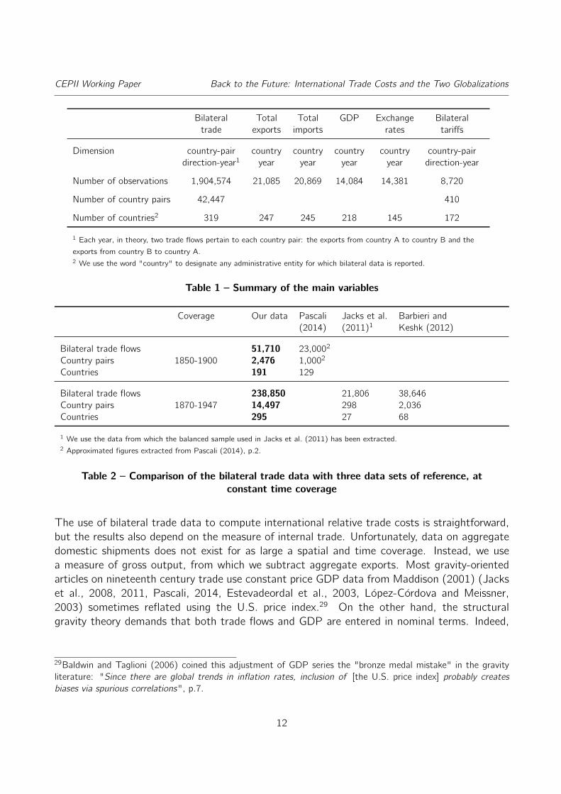
Table 1 provides a summary of the main variables. Table 2 compares our data with three bilateraltrade data sets of reference. In order for these comparisons to be meaningful, we compare eachof these data sets with the sub-sample of our own data that covers the same period.28 Atconstant time coverage and in terms of the number of observed trade flows, our data set istherefore more than twice as large as (Pascali, 2014), about 11 times larger than (Jacks et al.,2011) and more than 6 times the size of (Barbieri and Keshk, 2012).
26We discuss the measure of internal trade we use in Section 3.27Specifically, we use the median coefficient from their meta-analysis, restricted to the structural gravity estimatesidentified through tariff variation (see Table 5, p.33).28We restrict the samples to the years before 1948 because all the data sets rely on the same data from the IMFafter that point.
11
CEPII Working Paper Back to the Future: International Trade Costs and the Two Globalizations
Bilateral Total Total GDP Exchange Bilateraltrade exports imports rates tariffs
Dimension country-pair country country country country country-pairdirection-year1 year year year year direction-year
Number of observations 1,904,574 21,085 20,869 14,084 14,381 8,720
Number of country pairs 42,447 410
Number of countries2 319 247 245 218 145 172
1 Each year, in theory, two trade flows pertain to each country pair: the exports from country A to country B and the
exports from country B to country A.2 We use the word "country" to designate any administrative entity for which bilateral data is reported.
Table 1 – Summary of the main variables
Coverage Our data Pascali Jacks et al. Barbieri and(2014) (2011)1 Keshk (2012)
Bilateral trade flows 51,710 23,0002
Country pairs 1850-1900 2,476 1,0002
Countries 191 129
Bilateral trade flows 238,850 21,806 38,646Country pairs 1870-1947 14,497 298 2,036Countries 295 27 68
1 We use the data from which the balanced sample used in Jacks et al. (2011) has been extracted.2 Approximated figures extracted from Pascali (2014), p.2.
Table 2 – Comparison of the bilateral trade data with three data sets of reference, atconstant time coverage
The use of bilateral trade data to compute international relative trade costs is straightforward,but the results also depend on the measure of internal trade. Unfortunately, data on aggregatedomestic shipments does not exist for as large a spatial and time coverage. Instead, we usea measure of gross output, from which we subtract aggregate exports. Most gravity-orientedarticles on nineteenth century trade use constant price GDP data from Maddison (2001) (Jackset al., 2008, 2011, Pascali, 2014, Estevadeordal et al., 2003, López-Córdova and Meissner,2003) sometimes reflated using the U.S. price index.29 On the other hand, the structuralgravity theory demands that both trade flows and GDP are entered in nominal terms. Indeed,
29Baldwin and Taglioni (2006) coined this adjustment of GDP series the "bronze medal mistake" in the gravityliterature: "Since there are global trends in inflation rates, inclusion of [the U.S. price index] probably createsbiases via spurious correlations", p.7.
12
CEPII Working Paper Back to the Future: International Trade Costs and the Two Globalizations
the gravity equation is a function that allocates nominal expenditures across countries, i.e. thatallocates nominal GDP into nominal imports. We therefore rely exclusively on nominal series.
Internal trade, as any measure of trade, is a gross concept in the sense that it includes intermedi-ate goods. It should thus be measured as gross domestic tradable output, minus total exports.30
Unfortunately, reconstructions of national accounts have concentrated on GDP series that areby definition net of intermediary consumption. Our approach is to use the average ratio of grossoutput to value added taken from de Sousa et al. (2012) to scale up current price GDP dataand obtain an approximation of gross output.31 We finally subtract total exports and use theresulting series as our benchmark measure of internal trade.32
4. Estimation of the trade elasticity
The trade elasticity is a necessary parameter to infer trade costs from trade data. Indeed, astrong response of trade to trade costs translates in lower trade costs being inferred from thesame data. In the extreme case, if consumers are infinitely sensitive to trade costs, then theabsence of trade does not reveal prohibitive trade costs, but simply a total lack of interest forforeign goods. In our case, any observed reduction of trade costs can therefore be genuine, oran artifact due to a fall in the (absolute) trade elasticity over time. Checking for long run trendsin the trade elasticity is therefore crucial to establishing the robustness of our results. Beyondour direct interest, the trade elasticity is also a key parameter in the recent literature whichaims at recovering the welfare gains from trade. In particular, Arkolakis et al. (2012) showthat in a broad class of trade models two statistics are sufficient to calculate countries’ welfaregains from trade: the import openness ratio and the trade elasticity. Historical estimations ofthe trade elasticity are therefore a necessary prerequisite to any structural investigation of thewelfare gains associated with nineteenth century trade.
Head and Mayer (2014) show that in any trade model that yields structural gravity, the tradeelasticity is related to the parameter that governs the scope for trade gains. More precisely, theresponse of trade to trade costs decreases with the potential trade gains. It is thus necessary tolook into the models to understand the micro-level reasons for changes in the trade elasticity.
30Gross output = GDP + Intermediary consumption. Measuring internal trade as Gross output − exports isespecially relevant for countries that are very open to trade, as for some years, failing to adjust GDP for intermediateconsumption would result in negative internal trade. For further discussion, see Head and Mayer (2014), p.169.31Specifically, we aggregate their figures across industrial sectors to obtain an average ratio of 3.16. We then takethe product of this ratio and GDP as a measure of gross output.32We provide alternative results with internal trade measured as: Tradable GDP − exports. To do so, we decomposeGDP into a tradable (agriculture and industry) and a non-tradable component (services). We scale-up this datausing ratios of value added to gross production. For the industrial sector, we use the ratio from de Sousa et al.(2012). For agriculture, we use a ratio of 2.4 (INSEE, Compte provisoire de l’agriculture, May 2013). This comesat the cost of restricting the sample to 58% of its full potential. In Figure A.15, we estimate our world trade costindex using this alternative method.
13
CEPII Working Paper Back to the Future: International Trade Costs and the Two Globalizations
In the demand-side models of AvW (2003) (perfect competition) and Krugman (1980) (monop-olistic competition), the trade elasticity is linked to the elasticity of substitution across varieties(ε = 1 − σ). Countries trade to satisfy consumers’ love of variety. In turn, when varieties areclose substitutes (large σ), the incentives for trading narrow and the (absolute) trade elasticityincreases. An increasing similarity of the goods produced across countries would therefore leadto a rise of the trade elasticity. In supply-side models such as the Ricardian model (Eaton andKortum, 2002) and heterogeneous firms models (Chaney, 2008, Melitz and Ottaviano, 2008), θ(γ) is the parameter that governs the degree of heterogeneity of industries’ (Ricardo) or firms’productivity (heterogeneous firms). The less heterogeneity on the production side (large θ orγ), the smaller the scope for trade gains and the larger the trade elasticity. An homogenizationof industries’ or firms’ productivity would therefore lead to a rise of the trade elasticity.
We follow Romalis (2007) and use bilateral tariffs to identify the trade elasticity in both the crosssection and the time dimension using French data for 1829-1913. The identifying assumptionis that tariffs are pure cost shifters, i.e. that trade costs react one for one to changes in tariffs.We begin with the structural gravity equation:
Xi jt =Yit XjtPit Πjt
τ εi jt . (8)
We specify trade costs as follows:
τi jt = (1 + ti jt)×Distα1
i j × exp(α2 Coloi jt)× exp(α3 Comlangi j)
× exp(α4 Contii j)× ηi jt ,(9)
where ti jt is a measure of bilateral tariffs. Disti j is the population-weighted great-circle dis-tance. Coloi jt , Comlangi j and Contii j are three dummies that account for colonial relationship,common language and a shared border. ηi jt reflects the unobserved components of trade costs.
We estimate the trade elasticity using the ratio of bilateral customs duties to imports as aproxy for bilateral tariffs. A caveat should be noted: tariffs have an ambiguous link to theseratios. First, higher tariffs increase the value of the customs duties that are collected. At thesame time, tariffs reduce imports by making imported goods more expensive33. The resultingduties-to-imports ratios may therefore underestimate the actual level of protection. In turn, thetrade elasticities we estimate should be considered as lower bounds (in absolute terms).
33In particular, the prohibitive tariffs that were imposed on some products until the late nineteenth century resultin an underestimation of the actual level of protection. See the Irwin-Nye controversy (Nye, 1991, Irwin, 1993).
14
CEPII Working Paper Back to the Future: International Trade Costs and the Two Globalizations
We obtain the cross-section equation by plugging equation (9) into (8), taking logs and removingtime subscripts. We estimate the resulting equation separately for each year using OLS. Thenotation explicitly specifies that France is always the destination country:
lnXiFR = ε ln(1 + tiFR) + γ ln Yi + β1 lnDistiFR + β2 ColoiFR
+ β3 ComlangiFR + β4 ContiiFR + ln ηiFR.(10)
We use the notation βx = αx × ε, ∀ x ∈ {1, 2, 3, 4}. Yi is the GDP of country i . The error term(ηiFR) captures the bilateral components of trade costs that are not explicitly controlled for, aswell as origin countries’ outward multilateral resistance terms. As a result, the trade elasticitiesobtained from equation (10) cannot be considered as structural estimates.34
We also identify the trade elasticity in the time dimension, using decade-long intervals. This time,we keep the time subscripts and impose a set of origin-country fixed effects. The identificationtherefore entirely comes from the time dimension:
lnXiFRt = ε ln(1 + tiFRt) + FEiFR + γ1 ln Yit + γ2 ln YFRt
+ β2 ColoiFRt + ln ηiFRt .(11)
The error term (ηiFRt) captures the time-varying unobserved components of trade costs, as wellas the time-varying components of both inward and outward multilateral resistance terms. Thecoefficients estimated using equation (11) thus do not qualify as structural gravity estimates.
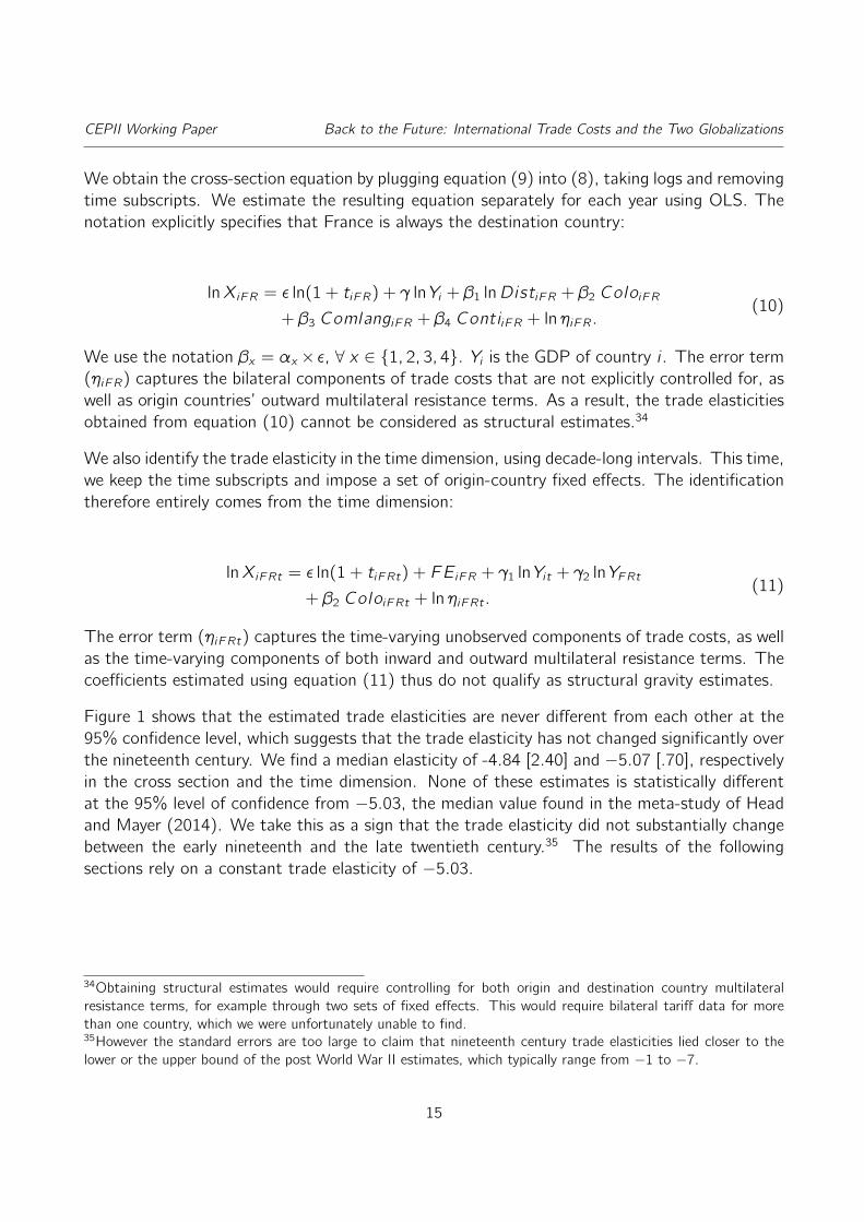
Figure 1 shows that the estimated trade elasticities are never different from each other at the95% confidence level, which suggests that the trade elasticity has not changed significantly overthe nineteenth century. We find a median elasticity of -4.84 [2.40] and −5.07 [.70], respectivelyin the cross section and the time dimension. None of these estimates is statistically differentat the 95% level of confidence from −5.03, the median value found in the meta-study of Headand Mayer (2014). We take this as a sign that the trade elasticity did not substantially changebetween the early nineteenth and the late twentieth century.35 The results of the followingsections rely on a constant trade elasticity of −5.03.
34Obtaining structural estimates would require controlling for both origin and destination country multilateralresistance terms, for example through two sets of fixed effects. This would require bilateral tariff data for morethan one country, which we were unfortunately unable to find.35However the standard errors are too large to claim that nineteenth century trade elasticities lied closer to thelower or the upper bound of the post World War II estimates, which typically range from −1 to −7.
15
CEPII Working Paper Back to the Future: International Trade Costs and the Two Globalizations
-20
-10
010
trade
ela
stic
ity
1830 1840 1850 1860 1870 1880 1890 1900 1910
Cross-section estimation Time series estimation (by decade)The shaded areas represent 95% confidence intervals
Figure 1 – Cross-sectional and longitudinal estimations of the trade elasticity: 1829-1913
5. World trade cost indices
Once equipped with a value for the trade elasticity, we can use equation (7) to compute tradecosts. We obtain more than 370,000 measures of trade costs for about 14,000 country pairs.Reporting all of the results would be impossible; instead, we report selected aggregates.
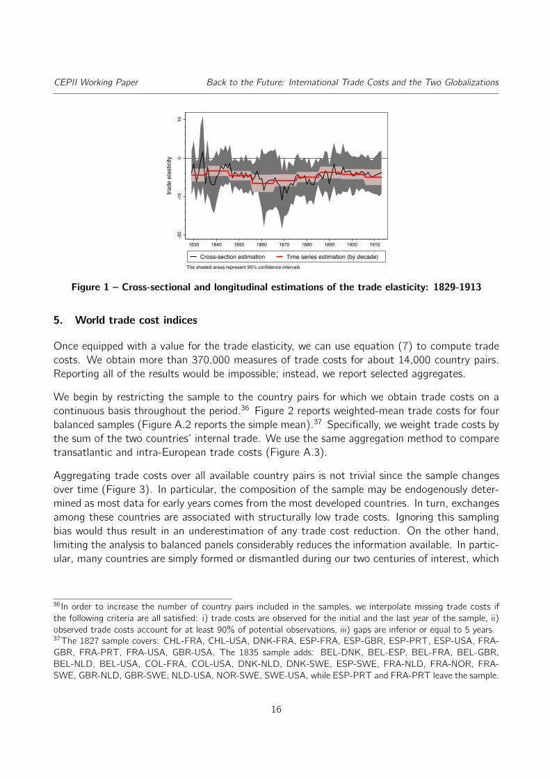
We begin by restricting the sample to the country pairs for which we obtain trade costs on acontinuous basis throughout the period.36 Figure 2 reports weighted-mean trade costs for fourbalanced samples (Figure A.2 reports the simple mean).37 Specifically, we weight trade costs bythe sum of the two countries’ internal trade. We use the same aggregation method to comparetransatlantic and intra-European trade costs (Figure A.3).
Aggregating trade costs over all available country pairs is not trivial since the sample changesover time (Figure 3). In particular, the composition of the sample may be endogenously deter-mined as most data for early years comes from the most developed countries. In turn, exchangesamong these countries are associated with structurally low trade costs. Ignoring this samplingbias would thus result in an underestimation of any trade cost reduction. On the other hand,limiting the analysis to balanced panels considerably reduces the information available. In partic-ular, many countries are simply formed or dismantled during our two centuries of interest, which
36In order to increase the number of country pairs included in the samples, we interpolate missing trade costs ifthe following criteria are all satisfied: i) trade costs are observed for the initial and the last year of the sample, ii)observed trade costs account for at least 90% of potential observations, iii) gaps are inferior or equal to 5 years.37The 1827 sample covers: CHL-FRA, CHL-USA, DNK-FRA, ESP-FRA, ESP-GBR, ESP-PRT, ESP-USA, FRA-GBR, FRA-PRT, FRA-USA, GBR-USA. The 1835 sample adds: BEL-DNK, BEL-ESP, BEL-FRA, BEL-GBR,BEL-NLD, BEL-USA, COL-FRA, COL-USA, DNK-NLD, DNK-SWE, ESP-SWE, FRA-NLD, FRA-NOR, FRA-SWE, GBR-NLD, GBR-SWE, NLD-USA, NOR-SWE, SWE-USA, while ESP-PRT and FRA-PRT leave the sample.
16
CEPII Working Paper Back to the Future: International Trade Costs and the Two Globalizations24
026
028
030
032
034
0
tarif
f equ
ival
ent (
%)
1840 1860 1880 1900 1920 1940 1960 1980 2000
1827 (11) 1835 (28) 1870 (93) 1921 (236)The legend reports the initial year of each sample (# of pairs in each sample in parenthesis)The two world wars are omitted from the samples
Figure 2 – Internal trade-weighted meantrade costs, balanced samples
4040
040
00
num
ber o
f obs
erva
tions
(log
sca
le)
1840 1860 1880 1900 1920 1940 1960 1980 2000
Figure 3 – Number of computed bilateraltrade costs
automatically rules them out from any balanced sample.38 We therefore propose an index oftrade costs that makes use of all of the information available while also partially controlling forthe sampling bias. Specifically, we decompose trade costs into a bilateral and a time effect:39
lnTCi jt = αi j FEi j + βt FEt + ηi jt . (12)
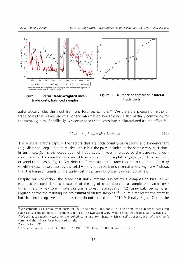
The bilateral effects capture the factors that are both country-pair-specific and time-invariant(e.g. distance, long-run cultural ties, etc.); but the pairs included in the sample vary over time.In turn, exp(βt) is the expectation of trade costs in year t relative to the benchmark year,conditional on the country pairs available in year t. Figure 4 plots exp(βt), which is our indexof world trade costs. Figure A.4 plots the former against a trade cost index that is obtained byweighting each observation by the total value of both partner’s internal trade. Figure A.4 showsthat the long-run trends of the trade cost index are not driven by small countries.
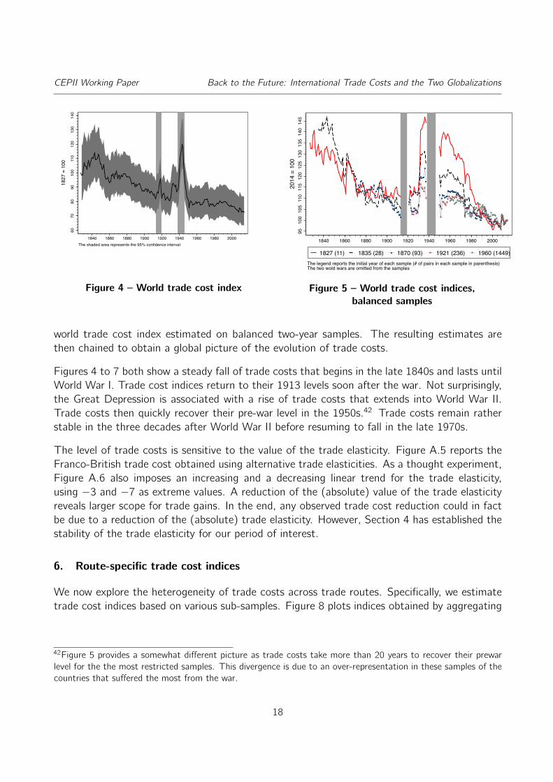
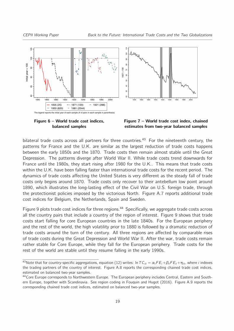
Despite our correction, the trade cost index remains subject to a composition bias, as weestimate the conditional expectation of the log of trade costs on a sample that varies overtime. The only way to eliminate this bias is to estimate equation (12) using balanced samples.Figure 5 shows the resulting indices estimated on five samples.40 Figure 6 replicates the exercisebut this time using five sub-periods that do not extend until 2014.41 Finally, Figure 7 plots the
38We compute 14 bilateral trade costs for 1827 and about 9,000 for 2014. Over time, the number of computedtrade costs tends to increase, to the exception of the two world wars, which temporarily reduce data availability.39We estimate equation (12) using the reghdfe command from Stata, which is itself a generalization of the xtreg,fecommand that allows for unbalanced panels.40see footnote 36.41These sub-periods are: 1835-1870, 1871-1912, 1921-1937, 1950-1980 and 1981-2014.
17
CEPII Working Paper Back to the Future: International Trade Costs and the Two Globalizations60
7080
9010
011
012
013
014
0
1827
= 1
00
1840 1860 1880 1900 1920 1940 1960 1980 2000The shaded area represents the 95% confidence interval
Figure 4 – World trade cost index95
100
105
110
115
120
125
130
135
140
145
2014
= 1
00
1840 1860 1880 1900 1920 1940 1960 1980 2000
1827 (11) 1835 (28) 1870 (93) 1921 (236) 1960 (1449)The legend reports the initial year of each sample (# of pairs in each sample in parenthesis)The two wold wars are omitted from the samples
Figure 5 – World trade cost indices,balanced samples
world trade cost index estimated on balanced two-year samples. The resulting estimates arethen chained to obtain a global picture of the evolution of trade costs.
Figures 4 to 7 both show a steady fall of trade costs that begins in the late 1840s and lasts untilWorld War I. Trade cost indices return to their 1913 levels soon after the war. Not surprisingly,the Great Depression is associated with a rise of trade costs that extends into World War II.Trade costs then quickly recover their pre-war level in the 1950s.42 Trade costs remain ratherstable in the three decades after World War II before resuming to fall in the late 1970s.
The level of trade costs is sensitive to the value of the trade elasticity. Figure A.5 reports theFranco-British trade cost obtained using alternative trade elasticities. As a thought experiment,Figure A.6 also imposes an increasing and a decreasing linear trend for the trade elasticity,using −3 and −7 as extreme values. A reduction of the (absolute) value of the trade elasticityreveals larger scope for trade gains. In the end, any observed trade cost reduction could in factbe due to a reduction of the (absolute) trade elasticity. However, Section 4 has established thestability of the trade elasticity for our period of interest.
6. Route-specific trade cost indices
We now explore the heterogeneity of trade costs across trade routes. Specifically, we estimatetrade cost indices based on various sub-samples. Figure 8 plots indices obtained by aggregating
42Figure 5 provides a somewhat different picture as trade costs take more than 20 years to recover their prewarlevel for the the most restricted samples. This divergence is due to an over-representation in these samples of thecountries that suffered the most from the war.
18
CEPII Working Paper Back to the Future: International Trade Costs and the Two Globalizations80
8590
9510
010
5
Initi
al y
ear =
100
1840 1860 1880 1900 1920 1940 1960 1980 2000
1835 (25) 1871 (120) 1921 (288)1950 (820) 1981 (2544)
The legend reports the initial year of each sample (# of pairs in each sample in parenthesis)
Figure 6 – World trade cost indices,balanced samples
2030
4050
6070
8090
100
110
1827
= 1
00
1840 1860 1880 1900 1920 1940 1960 1980 2000
Figure 7 – World trade cost index, chainedestimates from two-year balanced samples
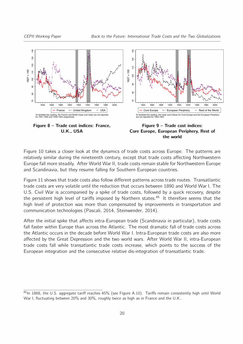
bilateral trade costs across all partners for three countries.43 For the nineteenth century, thepatterns for France and the U.K. are similar as the largest reduction of trade costs happensbetween the early 1850s and the 1870. Trade costs then remain almost stable until the GreatDepression. The patterns diverge after World War II. While trade costs trend downwards forFrance until the 1980s, they start rising after 1980 for the U.K.. This means that trade costswithin the U.K. have been falling faster than international trade costs for the recent period. Thedynamics of trade costs affecting the United States is very different as the steady fall of tradecosts only begins around 1870. Trade costs only recover to their antebellum low point around1890, which illustrates the long-lasting effect of the Civil War on U.S. foreign trade, throughthe protectionist policies imposed by the victorious North. Figure A.7 reports additional tradecost indices for Belgium, the Netherlands, Spain and Sweden.
Figure 9 plots trade cost indices for three regions.44 Specifically, we aggregate trade costs acrossall the country pairs that include a country of the region of interest. Figure 9 shows that tradecosts start falling for core European countries in the late 1840s. For the European peripheryand the rest of the world, the high volatility prior to 1880 is followed by a dramatic reduction oftrade costs around the turn of the century. All three regions are affected by comparable risesof trade costs during the Great Depression and World War II. After the war, trade costs remainrather stable for Core Europe, while they fall for the European periphery. Trade costs for therest of the world are stable until they resume falling in the early 1990s.
43Note that for country-specific aggregations, equation (12) writes: lnTCit = αiFEi +βtFEt+ηit , where i indexesthe trading partners of the country of interest. Figure A.8 reports the corresponding chained trade cost indices,estimated on balanced two-year samples.44Core Europe corresponds to Northwestern Europe. The European periphery includes Central, Eastern and South-ern Europe, together with Scandinavia. See region coding in Fouquin and Hugot (2016). Figure A.9 reports thecorresponding chained trade cost indices, estimated on balanced two-year samples.
19
CEPII Working Paper Back to the Future: International Trade Costs and the Two Globalizations70
8090
100
110
120
130
140
1827
= 1
00
1840 1860 1880 1900 1920 1940 1960 1980 2000
France United Kingdom USATo facilitate the reading, the French and British trade cost index are not reportedfor 1941-1945 and 1942-1944 respectively
Figure 8 – Trade cost indices: France,U.K., USA
7080
9010
011
012
013
0
1827
= 1
00
1840 1860 1880 1900 1920 1940 1960 1980 2000
Core Europe European Periphery Rest of the WorldTo facilitate the reading, the trade cost indices for Core Europe and the European Peripheryare not reported for 1943-1944
Figure 9 – Trade cost indices:Core Europe, European Periphery, Rest of
the world
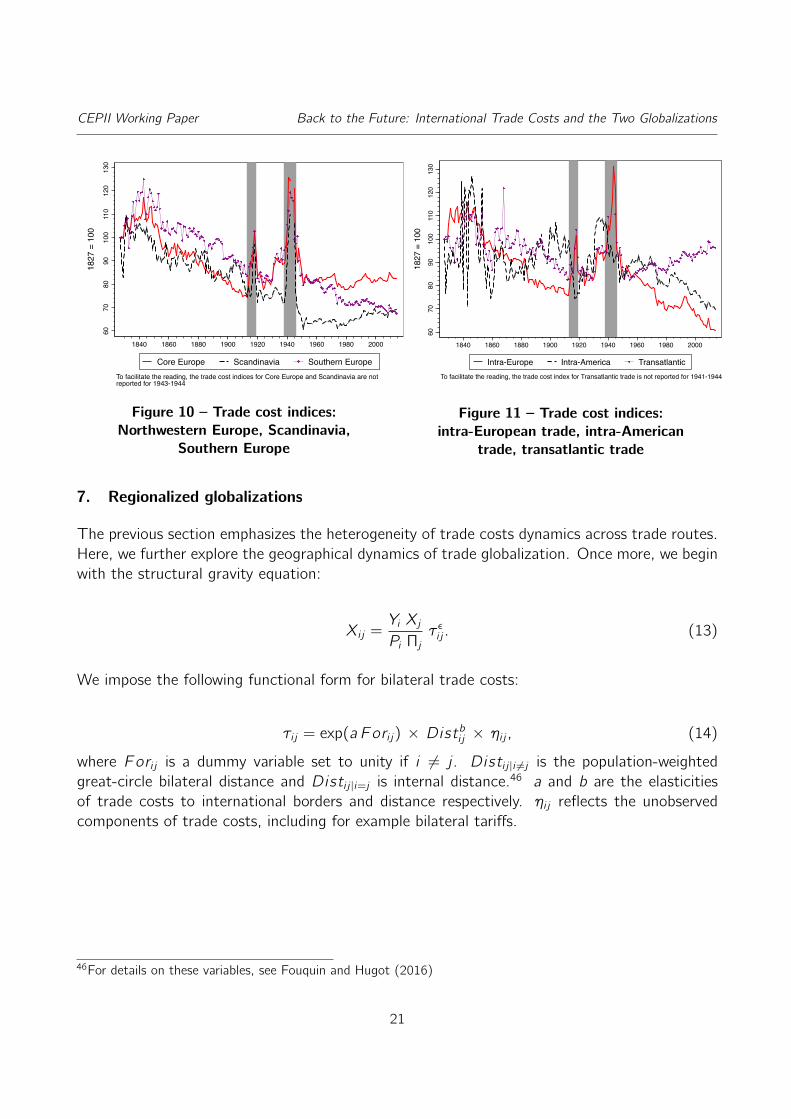
Figure 10 takes a closer look at the dynamics of trade costs across Europe. The patterns arerelatively similar during the nineteenth century, except that trade costs affecting NorthwesternEurope fall more steadily. After World War II, trade costs remain stable for Northwestern Europeand Scandinavia, but they resume falling for Southern European countries.
Figure 11 shows that trade costs also follow different patterns across trade routes. Transatlantictrade costs are very volatile until the reduction that occurs between 1890 and World War I. TheU.S. Civil War is accompanied by a spike of trade costs, followed by a quick recovery, despitethe persistent high level of tariffs imposed by Northern states.45 It therefore seems that thehigh level of protection was more than compensated by improvements in transportation andcommunication technologies (Pascali, 2014, Steinwender, 2014).
After the initial spike that affects intra-European trade (Scandinavia in particular), trade costsfall faster within Europe than across the Atlantic. The most dramatic fall of trade costs acrossthe Atlantic occurs in the decade before World War I. Intra-European trade costs are also moreaffected by the Great Depression and the two world wars. After World War II, intra-Europeantrade costs fall while transatlantic trade costs increase, which points to the success of theEuropean integration and the consecutive relative dis-integration of transatlantic trade.
45In 1868, the U.S. aggregate tariff reaches 45% (see Figure A.10). Tariffs remain consistently high until WorldWar I, fluctuating between 20% and 30%, roughly twice as high as in France and the U.K..
20
CEPII Working Paper Back to the Future: International Trade Costs and the Two Globalizations60
7080
9010
011
012
013
0
1827
= 1
00
1840 1860 1880 1900 1920 1940 1960 1980 2000
Core Europe Scandinavia Southern EuropeTo facilitate the reading, the trade cost indices for Core Europe and Scandinavia are notreported for 1943-1944
Figure 10 – Trade cost indices:Northwestern Europe, Scandinavia,
Southern Europe60
7080
9010
011
012
013
0
1827
= 1
00
1840 1860 1880 1900 1920 1940 1960 1980 2000
Intra-Europe Intra-America TransatlanticTo facilitate the reading, the trade cost index for Transatlantic trade is not reported for 1941-1944
Figure 11 – Trade cost indices:intra-European trade, intra-American
trade, transatlantic trade
7. Regionalized globalizations
The previous section emphasizes the heterogeneity of trade costs dynamics across trade routes.Here, we further explore the geographical dynamics of trade globalization. Once more, we beginwith the structural gravity equation:
Xi j =Yi XjPi Πj
τ εi j . (13)
We impose the following functional form for bilateral trade costs:
τi j = exp(a Fori j) × Distbij × ηi j , (14)
where Fori j is a dummy variable set to unity if i 6= j . Disti j |i 6=j is the population-weightedgreat-circle bilateral distance and Disti j |i=j is internal distance.46 a and b are the elasticitiesof trade costs to international borders and distance respectively. ηi j reflects the unobservedcomponents of trade costs, including for example bilateral tariffs.
46For details on these variables, see Fouquin and Hugot (2016)
21
CEPII Working Paper Back to the Future: International Trade Costs and the Two Globalizations
Plugging (14) into (13), taking logs and imposing origin and destination fixed effects to controlfor the monadic determinants of trade, we estimate equation (15), separately for each year,using the OLS estimator. The identification comes entirely from the cross-sectional variation:47
lnXi j = FEi + FEj + β1 Fori j + β2 lnDisti j + ln ηi j , (15)
where Xi j |i 6=j is bilateral trade and Xi j |i=j is internal trade. FEi and FEj are vectors of origin anddestination fixed effects. β1 = a× ε is the border effect and β2 = b× ε is the trade elasticity ofdistance. Note that the fixed effects perfectly control for the monadic determinants of trade,including multilateral resistance terms. Because the errors are likely correlated within countrypairs, we cluster the standard errors at the bilateral level.
7.1. Border effect
β1 can be interpreted as a border effect as it reflects the average trade reducing effect ofinternational borders, all monadic determinants of trade and distance being equal. We convertthe border effect into a tariff equivalent using the pure cost-shifter property of tariffs.48. Indeed,ad-valorem tariffs have a one for one relationship to trade costs. In turn, the error term ofequation (15) can be decomposed as follows:
ηi j = (1 + ti j)1 × Zi j , (16)
where ti j is the (unobserved) ad-valorem tariff imposed by j on imports from i . Zi j is a vectorof the other bilateral components of trade costs, together with their elasticities to trade costs.
The border effect we propose is equal to the tariff that would have the same trade reducingeffect as the average border. We therefore use the β1 estimated for each year via equation (15)to solve for the border effect (BE) in the following equation:
(1 + BE)ε = exp(β1). (17)
The resulting tariff-equivalent border effect, converted to a percentage, writes:
BE =
[exp
(β1
ε
)− 1
]× 100. (18)
47The identification of the border effect relies on a comparison of internal trade with bilateral trade as in Wei(1996), who extended the methodology introduced by McCallum (1995) for cases in which bilateral intra-nationaltrade flows are not available.48Figure A.11 reports the border effect as the exponential of β1. These values read as the number of times countriestrade more, on average, with themselves than with foreign partners, all monadic terms and distance being equal.
22
CEPII Working Paper Back to the Future: International Trade Costs and the Two Globalizations
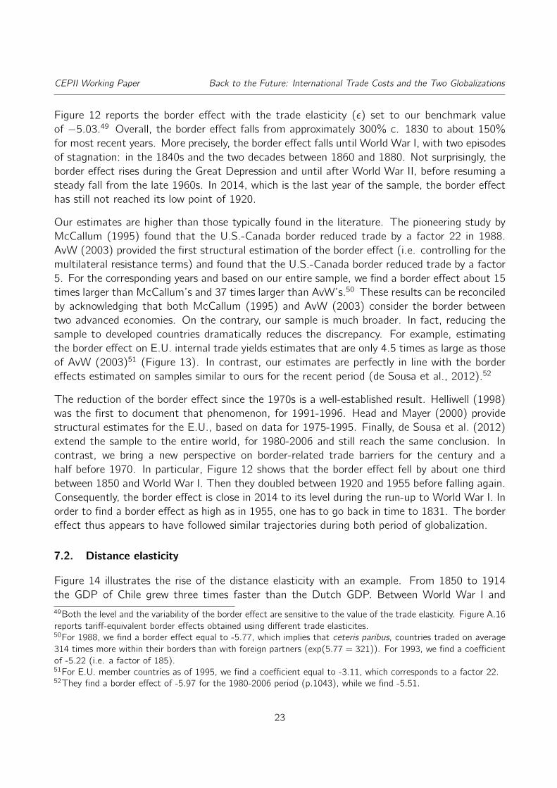
Figure 12 reports the border effect with the trade elasticity (ε) set to our benchmark valueof −5.03.49 Overall, the border effect falls from approximately 300% c. 1830 to about 150%for most recent years. More precisely, the border effect falls until World War I, with two episodesof stagnation: in the 1840s and the two decades between 1860 and 1880. Not surprisingly, theborder effect rises during the Great Depression and until after World War II, before resuming asteady fall from the late 1960s. In 2014, which is the last year of the sample, the border effecthas still not reached its low point of 1920.
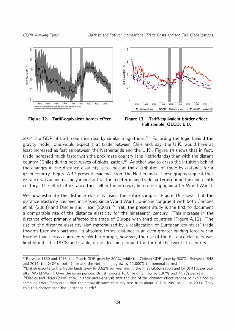
Our estimates are higher than those typically found in the literature. The pioneering study byMcCallum (1995) found that the U.S.-Canada border reduced trade by a factor 22 in 1988.AvW (2003) provided the first structural estimation of the border effect (i.e. controlling for themultilateral resistance terms) and found that the U.S.-Canada border reduced trade by a factor5. For the corresponding years and based on our entire sample, we find a border effect about 15times larger than McCallum’s and 37 times larger than AvW’s.50 These results can be reconciledby acknowledging that both McCallum (1995) and AvW (2003) consider the border betweentwo advanced economies. On the contrary, our sample is much broader. In fact, reducing thesample to developed countries dramatically reduces the discrepancy. For example, estimatingthe border effect on E.U. internal trade yields estimates that are only 4.5 times as large as thoseof AvW (2003)51 (Figure 13). In contrast, our estimates are perfectly in line with the bordereffects estimated on samples similar to ours for the recent period (de Sousa et al., 2012).52
The reduction of the border effect since the 1970s is a well-established result. Helliwell (1998)was the first to document that phenomenon, for 1991-1996. Head and Mayer (2000) providestructural estimates for the E.U., based on data for 1975-1995. Finally, de Sousa et al. (2012)extend the sample to the entire world, for 1980-2006 and still reach the same conclusion. Incontrast, we bring a new perspective on border-related trade barriers for the century and ahalf before 1970. In particular, Figure 12 shows that the border effect fell by about one thirdbetween 1850 and World War I. Then they doubled between 1920 and 1955 before falling again.Consequently, the border effect is close in 2014 to its level during the run-up to World War I. Inorder to find a border effect as high as in 1955, one has to go back in time to 1831. The bordereffect thus appears to have followed similar trajectories during both period of globalization.
7.2. Distance elasticity
Figure 14 illustrates the rise of the distance elasticity with an example. From 1850 to 1914the GDP of Chile grew three times faster than the Dutch GDP. Between World War I and49Both the level and the variability of the border effect are sensitive to the value of the trade elasticity. Figure A.16reports tariff-equivalent border effects obtained using different trade elasticites.50For 1988, we find a border effect equal to -5.77, which implies that ceteris paribus, countries traded on average314 times more within their borders than with foreign partners (exp(5.77 = 321)). For 1993, we find a coefficientof -5.22 (i.e. a factor of 185).51For E.U. member countries as of 1995, we find a coefficient equal to -3.11, which corresponds to a factor 22.52They find a border effect of -5.97 for the 1980-2006 period (p.1043), while we find -5.51.
23
CEPII Working Paper Back to the Future: International Trade Costs and the Two Globalizations10
015
020
025
030
035
0
tarif
f equ
ival
ent (
%)
1840 1860 1880 1900 1920 1940 1960 1980 2000The shaded area represents the 95% confidence intervalStandard errors clustered at the bilateral level
Figure 12 – Tariff-equivalent border effect
010
020
030
040
0ta
riff e
quiva
lent
(%)
1840 1860 1880 1900 1920 1940 1960 1980 2000
All observations OECD (1964 members) EU (1995 members)
Figure 13 – Tariff-equivalent border effect:Full sample, OECD, E.U.
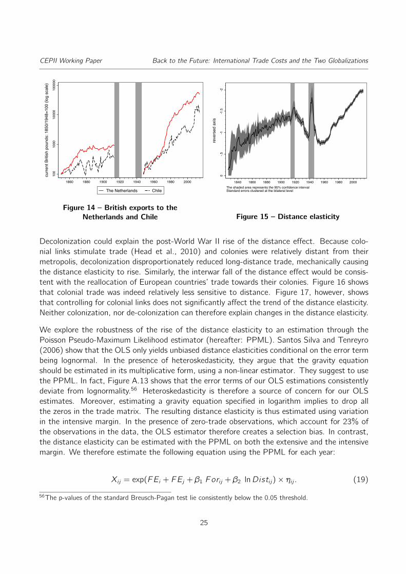
2014 the GDP of both countries rose by similar magnitudes.53 Following the logic behind thegravity model, one would expect that trade between Chile and, say, the U.K. would have atleast increased as fast as between the Netherlands and the U.K.. Figure 14 shows that in fact,trade increased much faster with the proximate country (the Netherlands) than with the distantcountry (Chile) during both waves of globalization.54 Another way to grasp the intuition behindthe changes in the distance elasticity is to look at the distribution of trade by distance for agiven country. Figure A.17 presents evidence from the Netherlands. These graphs suggest thatdistance was an increasingly important factor in determining trade patterns during the nineteenthcentury. The effect of distance then fell in the interwar, before rising again after World War II.
We now estimate the distance elasticity using the entire sample. Figure 15 shows that thedistance elasticity has been increasing since World War II, which is congruent with both Combeset al. (2008) and Disdier and Head (2008).55 Yet, the present study is the first to documenta comparable rise of the distance elasticity for the nineteenth century. This increase in thedistance effect primarily affected the trade of Europe with third countries (Figure A.12). Therise of the distance elasticity also materialized by a reallocation of European countries’ tradetowards European partners. In absolute terms, distance is an even greater binding force withinEurope than across continents. Within Europe, however, the rise of the distance elasticity waslimited until the 1870s and stable, if not declining around the turn of the twentieth century.
53Between 1850 and 1913, the Dutch GDP grew by 300%, while the Chilean GDP grew by 900%. Between 1948and 2014, the GDP of both Chile and the Netherlands grew by 11,000% (in nominal terms).54British exports to the Netherlands grew by 3.52% per year during the First Globalization and by 10.41% per yearafter World War II. Over the same periods, British exports to Chile only grew by 1.97% and 7.87% per year.55Disdier and Head (2008) show in their meta-analysis that the rise of the distance effect cannot be explained bysampling error. They argue that the actual distance elasticity rose from about -0.7 in 1960 to -1.1 in 2000. Theycoin this phenomenon the "distance puzzle".
24
CEPII Working Paper Back to the Future: International Trade Costs and the Two Globalizations10
010
0010
000
1000
00
curre
nt B
ritis
h po
unds
: 185
0/19
48=1
00 (l
og s
cale
)
1860 1880 1900 1920 1940 1960 1980 2000
The Netherlands Chile
Figure 14 – British exports to theNetherlands and Chile
-2-1
.5-1
-.50
reve
rsed
axi
s
1840 1860 1880 1900 1920 1940 1960 1980 2000The shaded area represents the 95% confidence intervalStandard errors clustered at the bilateral level
Figure 15 – Distance elasticity
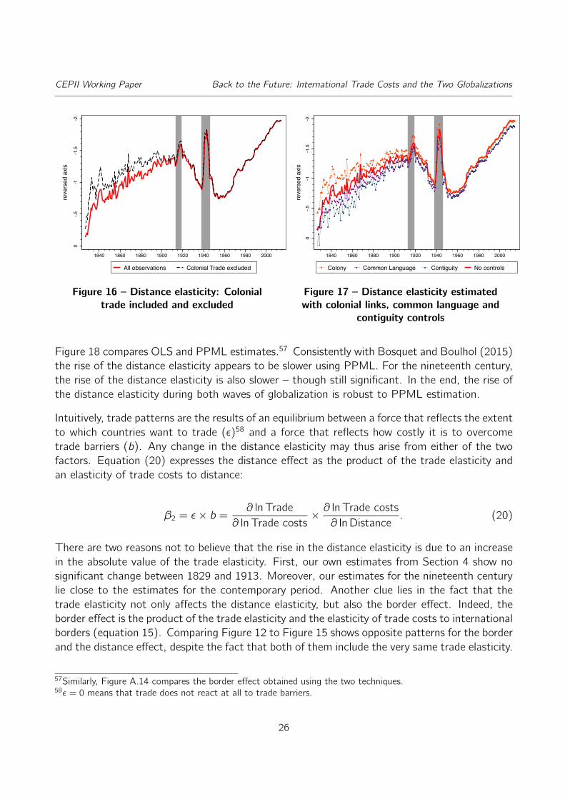
Decolonization could explain the post-World War II rise of the distance effect. Because colo-nial links stimulate trade (Head et al., 2010) and colonies were relatively distant from theirmetropolis, decolonization disproportionately reduced long-distance trade, mechanically causingthe distance elasticity to rise. Similarly, the interwar fall of the distance effect would be consis-tent with the reallocation of European countries’ trade towards their colonies. Figure 16 showsthat colonial trade was indeed relatively less sensitive to distance. Figure 17, however, showsthat controlling for colonial links does not significantly affect the trend of the distance elasticity.Neither colonization, nor de-colonization can therefore explain changes in the distance elasticity.
We explore the robustness of the rise of the distance elasticity to an estimation through thePoisson Pseudo-Maximum Likelihood estimator (hereafter: PPML). Santos Silva and Tenreyro(2006) show that the OLS only yields unbiased distance elasticities conditional on the error termbeing lognormal. In the presence of heteroskedasticity, they argue that the gravity equationshould be estimated in its multiplicative form, using a non-linear estimator. They suggest to usethe PPML. In fact, Figure A.13 shows that the error terms of our OLS estimations consistentlydeviate from lognormality.56 Heteroskedasticity is therefore a source of concern for our OLSestimates. Moreover, estimating a gravity equation specified in logarithm implies to drop allthe zeros in the trade matrix. The resulting distance elasticity is thus estimated using variationin the intensive margin. In the presence of zero-trade observations, which account for 23% ofthe observations in the data, the OLS estimator therefore creates a selection bias. In contrast,the distance elasticity can be estimated with the PPML on both the extensive and the intensivemargin. We therefore estimate the following equation using the PPML for each year:
Xi j = exp(FEi + FEj + β1 Fori j + β2 lnDisti j)× ηi j . (19)
56The p-values of the standard Breusch-Pagan test lie consistently below the 0.05 threshold.
25
CEPII Working Paper Back to the Future: International Trade Costs and the Two Globalizations-2
-1.5
-1-.5
0
reve
rsed
axi
s
1840 1860 1880 1900 1920 1940 1960 1980 2000
All observations Colonial Trade excluded
Figure 16 – Distance elasticity: Colonialtrade included and excluded
-2-1
.5-1
-.50
reve
rsed
axi
s
1840 1860 1880 1900 1920 1940 1960 1980 2000
Colony Common Language Contiguity No controls
Figure 17 – Distance elasticity estimatedwith colonial links, common language and
contiguity controls
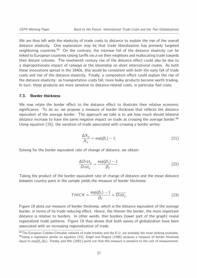
Figure 18 compares OLS and PPML estimates.57 Consistently with Bosquet and Boulhol (2015)the rise of the distance elasticity appears to be slower using PPML. For the nineteenth century,the rise of the distance elasticity is also slower – though still significant. In the end, the rise ofthe distance elasticity during both waves of globalization is robust to PPML estimation.
Intuitively, trade patterns are the results of an equilibrium between a force that reflects the extentto which countries want to trade (ε)58 and a force that reflects how costly it is to overcometrade barriers (b). Any change in the distance elasticity may thus arise from either of the twofactors. Equation (20) expresses the distance effect as the product of the trade elasticity andan elasticity of trade costs to distance:
β2 = ε× b =∂ lnTrade
∂ lnTrade costs×∂ lnTrade costs∂ lnDistance
. (20)
There are two reasons not to believe that the rise in the distance elasticity is due to an increasein the absolute value of the trade elasticity. First, our own estimates from Section 4 show nosignificant change between 1829 and 1913. Moreover, our estimates for the nineteenth centurylie close to the estimates for the contemporary period. Another clue lies in the fact that thetrade elasticity not only affects the distance elasticity, but also the border effect. Indeed, theborder effect is the product of the trade elasticity and the elasticity of trade costs to internationalborders (equation 15). Comparing Figure 12 to Figure 15 shows opposite patterns for the borderand the distance effect, despite the fact that both of them include the very same trade elasticity.
57Similarly, Figure A.14 compares the border effect obtained using the two techniques.58ε = 0 means that trade does not react at all to trade barriers.
26
CEPII Working Paper Back to the Future: International Trade Costs and the Two Globalizations
We are thus left with the elasticity of trade costs to distance to explain the rise of the overalldistance elasticity. One explanation may be that trade liberalization has primarily targetedneighboring countries.59 On the contrary, the interwar fall of the distance elasticity can belinked to European countries raising tariffs vis-à-vis their neighbors and reallocating trade towardstheir distant colonies. The nineteenth century rise of the distance effect could also be due toa disproportionate impact of railways or the steamship on short international routes. As boththese innovations spread in the 1840s, this would be consistent with both the early fall of tradecosts and rise of the distance elasticity. Finally, a composition effect could explain the rise ofthe distance elasticity: as transportation costs fall, more bulky products become worth trading.In turn, these products are more sensitive to distance-related costs, in particular fuel costs.
7.3. Border thickness
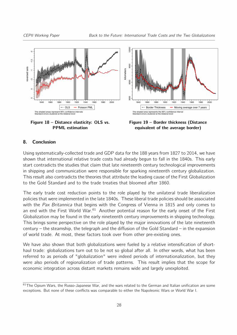
We now relate the border effect to the distance effect to illustrate their relative economicsignificance. To do so, we propose a measure of border thickness that reflects the distanceequivalent of the average border. The approach we take is to ask how much should bilateraldistance increase to have the same negative impact on trade as crossing the average border.60
Using equation (15), the variation of trade associated with crossing a border writes:
∆Xi jXi j
= exp(β1)− 1. (21)
Solving for the border equivalent rate of change of distance, we obtain:
∆Disti jDisti j
=exp(β1)− 1
β2
. (22)
Taking the product of the border equivalent rate of change of distance and the mean distancebetween country pairs in the sample yields the measure of border thickness:
THICK =exp(β1)− 1
β2
×Disti j . (23)
Figure 19 plots our measure of border thickness, which is the distance equivalent of the averageborder, in terms of its trade reducing effect. Hence, the thinner the border, the more importantdistance is relative to borders. In other words, thin borders (lower part of the graph) revealregionalized trade patterns. Figure 19 thus shows that both waves of globalization have beenassociated with an increasing regionalization of trade.59The European Cobden-Chevalier network of trade treaties and the E.U. are probably the most striking examples.60Using a regression similar to equation (15), Engel and Rogers (1996) propose a measure of border thicknessequal to exp(β1/β2). Parsley and Wei (2001) point out that this measure is sensitive to the unit of measurement.
27
CEPII Working Paper Back to the Future: International Trade Costs and the Two Globalizations-2
-1.5
-1-.5
0.5
reve
rsed
axis
1840 1860 1880 1900 1920 1940 1960 1980 2000
OLS Poisson PMLThe shaded areas represent 95% confidence intervalsStandard errors clustered at the bilateral level
Figure 18 – Distance elasticity: OLS vs.PPML estimation
3000
6000
9000
1200
0
kilo
met
ers
1840 1860 1880 1900 1920 1940 1960 1980 2000
Border Thickness Moving average over 7 yearsThe shaded area represents the 95% confidence intervalStandard errors clustered at the bilateral level
Figure 19 – Border thickness (Distanceequivalent of the average border)
8. Conclusion
Using systematically-collected trade and GDP data for the 188 years from 1827 to 2014, we haveshown that international relative trade costs had already begun to fall in the 1840s. This earlystart contradicts the studies that claim that late nineteenth century technological improvementsin shipping and communication were responsible for sparking nineteenth century globalization.This result also contradicts the theories that attribute the leading cause of the First Globalizationto the Gold Standard and to the trade treaties that bloomed after 1860.
The early trade cost reduction points to the role played by the unilateral trade liberalizationpolicies that were implemented in the late 1840s. These liberal trade policies should be associatedwith the Pax Britannica that begins with the Congress of Vienna in 1815 and only comes toan end with the First World War.61 Another potential reason for the early onset of the FirstGlobalization may be found in the early nineteenth century improvements in shipping technology.This brings some perspective on the role played by the major innovations of the late nineteenthcentury – the steamship, the telegraph and the diffusion of the Gold Standard – in the expansionof world trade. At most, these factors took over from other pre-existing ones.
We have also shown that both globalizations were fueled by a relative intensification of short-haul trade: globalizations turn out to be not so global after all. In other words, what has beenreferred to as periods of "globalization" were indeed periods of internationalization, but theywere also periods of regionalization of trade patterns. This result implies that the scope foreconomic integration across distant markets remains wide and largely unexploited.
61The Opium Wars, the Russo-Japanese War, and the wars related to the German and Italian unification are someexceptions. But none of these conflicts was comparable to either the Napoleonic Wars or World War I.
28
CEPII Working Paper Back to the Future: International Trade Costs and the Two Globalizations
References
Accominotti, Olivier and Marc Flandreau, “Does Bilateralism Promote Trade? NineteenthCentury Liberalization Revisited,” Working paper 5423, CEPR Jan. 2006.
Allen, Treb, Costas Arkolakis, and Yuta Takahashi, “Universal Gravity,” Working paper20787, NBER Dec. 2014.
Anderson, James E. and Eric van Wincoop, “Gravity with Gravitas: A Solution to the BorderPuzzle,” American Economic Review, Mar. 2003, 93 (1), 170–192.
Anderson, James E. and Eric van Wincoop, “Trade costs,” Journal of Economic Literature,Sep. 2004, 42 (3), 691–751.
Arkolakis, Costas, Arnaud Costinot, and Andrés Rodríguez Clare, “New Trade Models,Same Old Gains?,” American Economic Review, Aug. 2012, 102 (1), 94–130.
Baldwin, Richard and Daria Taglioni, “Gravity for Dummies and Dummies for Gravity Equa-tions,” Working paper 5850, CEPR Sep. 2006.
Barbieri, Katherine and Omar Keshk, “Correlates of War Project Trade Data set,” 2012,version 3.0. Available online: http://correlatesofwar.org.
Bosquet, Clément and Hervé Boulhol, “What is Really Puzzling about the "Distance Puzzle",”Review of World Economics, 2015, 151 (1), 1–21.
Broda, Christian and David E. Weinstein, “Globalization and the Gains from Variety,” Quar-terly Journal of Economics, May 2006, 121 (2), 541–585.
Bulbeck, David, Anthony Reid, Lay Cheng Tan, and Yiqu Wu, Southeast Asian Exportssince the 14th Century: Cloves, Pepper, Coffee, and Sugar, Leiden, The Netherlands: KITLVPress, 1998.
Chaney, Thomas, “Distorted Gravity: The Intensive and Extensive Margins of InternationalTrade,” American Economic Review, Sep. 2008, 98 (4), 1707–1721.
Coleman, Andrew, “The Pitfalls of Estimating Transactions Costs from Price data: Evidencefrom Trans-Atlantic Gold-point Arbitrage, 1886-1905,” Explorations in Economic History,2007, 44, 387–410.
Combes, Pierre-Philippe, Thierry Mayer, and Jacques-François Thisse, Economic Geog-raphy: The Integration of Regions and Nations, Princeton, N.J., USA: Princeton UniversityPress, 2008.
de Sousa, José, Thierry Mayer, and Soledad Zignago, “Market Access in Global and RegionalTrade,” Regional Science and Urban Economics, Nov. 2012, 42 (6), 1037–1052.
Disdier, Anne-Célia and Keith Head, “The Puzzling Persistence of the Distance Effect onBilateral Trade,” Review of Economics and Statistics, Feb. 2008, 90 (1), 37–48.
Dobado-González, Rafael, Alfredo García-Hiernaux, and David E. Guerrero, “The Integra-tion of Grain Markets in the Eighteenth Century: Early Rise of Globalization in the West,”Journal of Economic History, Sep. 2012, 72 (3), 671–707.
29
CEPII Working Paper Back to the Future: International Trade Costs and the Two Globalizations
Eaton, Jonathan and Samuel Kortum, “Technology, Geograpy and Trade,” Econometrica,Sep. 2002, 70 (5), 1741–1779.
Eaton, Jonhatan, Samuel Kortum, Brent Neiman, and John Romalis, “Trade and the GlobalRecession,” Working paper 16666, NBER Jan. 2011.
Engel, Charles and John H. Rogers, “How Wide is the Border?,” American Economic Review,1996, 86 (5), 1112–1125.
Estevadeordal, Antoni, Brian Frantz, and Alan M. Taylor, “The Rise and Fall of WorldTrade: 1870-1939,” Quarterly Journal of Economics, May 2003, 118 (2), 359–407.
Földvári, Péter and Bas van Leeuwen, “Markets in Ancient Societies? The Structural Analysisof Babylonian Price Data,” Working paper 2000.
Fouquin, Michel and Jules Hugot, “Two Centuries of Bilateral Trade and Gravity data: 1827-2012,” Working paper 2016-14, CEPII May 2016.
Hamilton, Earl J., American Treasure and the Price Revolution in Spain, 1501-1650, Cam-bridge, M.A., USA: Harvard University Press, 1934.
Harley, C. Knick, “Ocean Freight Rates and Productivity, 1740-1913: The Primacy of Me-chanical Invention Reaffirmed,” Journal of Economic History, Dec. 1988, 48 (4), 851–876.
Head, Keith and John Ries, “ Increasing Returns versus National Product Differentiation as anExplanation for the Pattern of U.S.-Canada Trade,” American Economic Review, Sep. 2001,91 (4), 858–876.
Head, Keith and Thierry Mayer, “Non-Europe: The Magnitude and Causes of Market Frag-mentation in the E.U.,” Review of World Economics, 2000, 136 (2), 284–314.
Head, Keith and Thierry Mayer, “What Separates Us? Sources of Resistance to Globaliza-tion,” Canadian Journal of Economics, Nov. 2013, 46 (4), 1196–1231.
Head, Keith and Thierry Mayer, “Gravity Equations: Workhorse, Toolkit, and Cookbook,”in Gita Gopinath, Elhanan Helpman, and Kenneth Rogoff, eds., vol. 4 of the Handbook ofInternational Economics, Amsterdam, The Netherlands: Elsevier, 2014, pp. 131–195.
Head, Keith, Thierry Mayer, and John Ries, “The Erosion of Colonial Trade Linkages AfterIndependence,” Journal of International Economics, 2010, 81 (1), 1–14.
Helliwell, John F., How Much Do National Borders Matter?, Washington, D.C., USA.: Brook-ings Institution, 1998.
Helpman, Elhanan, “ Imperfect Competition and International Trade: Evicence from FourteenIndustrial Countries,” Journal of the Japanese and International Economies, 1987, 1, 62–81.
Irwin, Douglas A., “Free Trade and Protection in Nineteenth-Century Britain and France Re-visited: A Comment on Nye,” Journal of Economic History, Mar. 1993, 53 (1), 146–152.
Jacks, David S., “Market Integration in the North and Baltic Seas, 1500-1800,” Journal ofEuropean Economic History, 2004, 33 (3), 285–329.
Jacks, David S., “ Intra- and International Commodity Market Integration in the Atlantic Econ-omy, 1800-1913,” Explorations in Economic History, 2005, 42, 381–413.
30
CEPII Working Paper Back to the Future: International Trade Costs and the Two Globalizations
Jacks, David S., Christopher M. Meissner, and Dennis Novy, “Trade Costs: 1870-2000,”American Economic Review: Papers and Proceedings, 2008, 98 (2), 529–534.
Jacks, David S., Christopher M. Meissner, and Dennis Novy, “Trade Booms, Trade Busts,and Trade Costs,” Journal of International Economics, 2011, 83 (2), 185–201.
Krugman, Paul, “Scale Economies, Product Differentiation, and the Pattern of Trade,” Amer-ican Economic Review, Dec. 1980, 70 (5), 950–959.
Lampe, Markus, “Effects of Bilateralism and the MFN Clause on International Trade: Evidencefor the Cobden-Chevalier Network, 1860-1875,” Journal of Economic History, 2009, 69 (4),1012–1040.
López-Córdova, J. Ernersto and Christopher Meissner, “Exchange-Rate Regimes and Inter-national Trade: Evidence from the Classical Gold Standard Era,” American Economic Review,Mar. 2003, 93 (1), 344–353.
Maddison, Angus, The World Economy: A Millenial Perspective, Paris, France: DevelopmentCentre Studies - OECD, 2001.
McCallum, John, “National Borders Matter: Canada-U.S. Regional Trade Patterns,” AmericanEconomic Review, Jun. 1995, 85 (3), 615–623.
Melitz, Marc J. and Gianmarco I. P. Ottaviano, “Market Size, Trade, and Productivity,”Review of Economic Studies, 2008, 75 (1), 295–316.
Novy, Dennis, “ Is the Iceberg Melting Less Quickly? International Trade Costs after World WarII,” Warwick Economic Research Papers 764, Warwick University 2007.
Novy, Dennis, “Gravity Redux: Measuring International Trade Costs with Panel Data,” Eco-nomic Inquiry, Jan. 2013, 51 (1), 101–121.
Nye, John Vincent, “The Myth of Free-trade Britain and Fortress France: Tariffs and Tradein the Nineteenth Century,” Journal of Economic History, Mar. 1991, 51 (1), 23–46.
O’Rourke, Kevin H., “The Worldwide Economic Impact of the French Revolutionary andNapoleonic Wars: 1793-1815,” Journal of Global History, Mar. 2006, 1 (1), 123–149.
O’Rourke, Kevin H. and Jeffrey G. Williamson, “Late Nineteenth-Century Anglo-AmericanFactor-Price Convergence: Were Heckscher and Ohlin Right?,” Journal of Economic History,Dec. 1994, 54 (4), 892–916.
O’Rourke, Kevin H. and Jeffrey G. Williamson, “When did Globalisation Begin?,” EuropeanReview of Economic History, Feb. 2002, 6, 23–50.
Parsley, David C. and Shang-Jin Wei, “Explaining the Border Effect: The Role of ExchangeRate Variability, Shipping Costs and Geography,” Journal of International Economics, 2001,55 (1), 87–105.
Pascali, Luigi, “The Wind of Change: Maritime Technology, Trade and Economic Develop-ment,” Working paper 1049, Warwick economic research papers Jun. 2014.
Romalis, John, “NAFTA’s and CUFTA’s Impact on International Trade,” The Review of Eco-nomics and Statistics, Aug. 2007, 89 (3), 416–435.
31
CEPII Working Paper Back to the Future: International Trade Costs and the Two Globalizations
Rönnbäck, Klas, “ Integration of Global Commodity Markets in the Early Modern Era,” EuropeanReview of Economic History, 2009, 13, 95–120.
Santos Silva, João M. C. and Silvana Tenreyro, “The Log of Gravity,” The Review of Eco-nomics and Statistics, Nov. 2006, 88 (4), 641–658.
Sharp, Paul, “’1846 and All That’: The Rise and Fall of British Wheat Protection in theNineteenth Century,” Agricultural History Review, 2010, 58 (1), 76–94.
Sharp, Paul and Jacob Weisdorf, “Globalization Revisited: Market Integration and the WheatTrade between North America and Britain from the Eighteenth Century,” Explorations inEconomic History, Jan. 2013, 50 (1), 88–98.
Solar, Peter M., “Opening to the East: Shipping between Europe and Asia,1770-1830,” Journalof Economic History, Sep. 2013, 73 (3), 625–661.
Steinwender, Claudia, “ Information Frictions and the Law of One Price: "When the Statesand the Kingdom Became United",” Working paper, London School of Economics Apr. 2014.
Wei, Shang-Jin, “ Intra-national versus International Trade: How Stubborn are Nations in GlobalIntegration?,” Working paper 5531, NBER Apr. 1996.
32
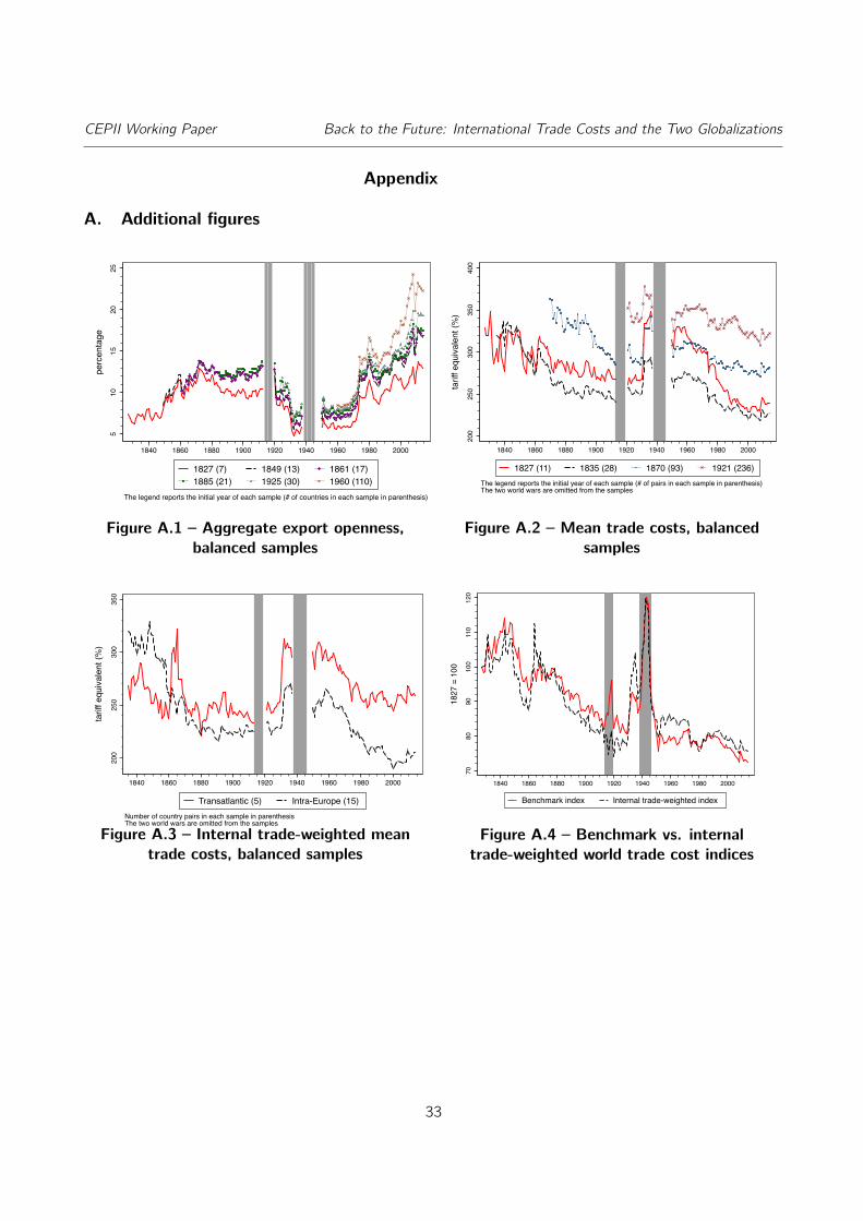
CEPII Working Paper Back to the Future: International Trade Costs and the Two Globalizations
Appendix
A. Additional figures
510
1520
25
perc
enta
ge
1840 1860 1880 1900 1920 1940 1960 1980 2000
1827 (7) 1849 (13) 1861 (17)1885 (21) 1925 (30) 1960 (110)
The legend reports the initial year of each sample (# of countries in each sample in parenthesis)
Figure A.1 – Aggregate export openness,balanced samples
200
250
300
350
400
tarif
f equ
ival
ent (
%)
1840 1860 1880 1900 1920 1940 1960 1980 2000
1827 (11) 1835 (28) 1870 (93) 1921 (236)The legend reports the initial year of each sample (# of pairs in each sample in parenthesis)The two world wars are omitted from the samples
Figure A.2 – Mean trade costs, balancedsamples
200
250
300
350
tarif
f equ
ival
ent (
%)
1840 1860 1880 1900 1920 1940 1960 1980 2000
Transatlantic (5) Intra-Europe (15)Number of country pairs in each sample in parenthesisThe two world wars are omitted from the samples
Figure A.3 – Internal trade-weighted meantrade costs, balanced samples
7080
9010
011
012
0
1827
= 1
00
1840 1860 1880 1900 1920 1940 1960 1980 2000
Benchmark index Internal trade-weighted index
Figure A.4 – Benchmark vs. internaltrade-weighted world trade cost indices
33
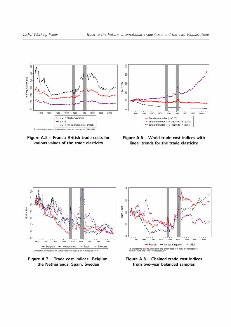
CEPII Working Paper Back to the Future: International Trade Costs and the Two Globalizations0
100
200
300
400
500
600
tarif
f equ
ival
ent (
%)
1840 1860 1880 1900 1920 1940 1960 1980 2000
ε = -5.03 (benchmark)ε = -3ε = -7 (as in Jacks et al., 2008)
To facilitate the reading, trade costs for are not reported for 1941-1946
Figure A.5 – Franco-British trade costs forvarious values of the trade elasticity
010
020
030
040
050
0
1827
= 1
00
1840 1860 1880 1900 1920 1940 1960 1980 2000
Benchmark index (ε=-5.03)Linear trend for ε: -7 (1827) to -3 (2014)Linear trend for ε: -3 (1827) to -7 (2014)
Figure A.6 – World trade cost indices withlinear trends for the trade elasticity
5060
7080
9010
011
012
0
1835
= 1
00
1840 1860 1880 1900 1920 1940 1960 1980 2000
Belgium Netherlands Spain SwedenTo facilitate the reading, the Dutch trade cost index is not reported for 1918
Figure A.7 – Trade cost indices: Belgium,the Netherlands, Spain, Sweden
6080
100
120
140
1827
= 1
00
1840 1860 1880 1900 1920 1940 1960 1980 2000
France United Kingdom USATo facilitate the reading, the French and British trade cost index are not reportedfor 1941-1946 and 1941-1945 respectively
Figure A.8 – Chained trade cost indicesfrom two-year balanced samples
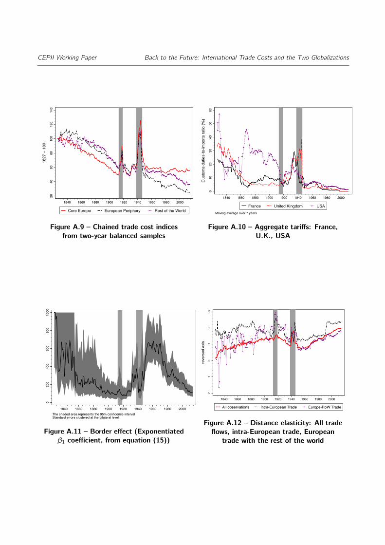
CEPII Working Paper Back to the Future: International Trade Costs and the Two Globalizations20
4060
8010
012
014
0
1827
= 1
00
1840 1860 1880 1900 1920 1940 1960 1980 2000
Core Europe European Periphery Rest of the World
Figure A.9 – Chained trade cost indicesfrom two-year balanced samples
010
2030
4050
60
Cus
tom
s du
ties-
to-im
ports
ratio
(%)
1840 1860 1880 1900 1920 1940 1960 1980 2000
France United Kingdom USAMoving average over 7 years
Figure A.10 – Aggregate tariffs: France,U.K., USA
020
040
060
080
010
00
1840 1860 1880 1900 1920 1940 1960 1980 2000The shaded area represents the 95% confidence intervalStandard errors clustered at the bilateral level
Figure A.11 – Border effect (Exponentiatedβ1 coefficient, from equation (15))
-3-2
-10
12
reve
rsed
axi
s
1840 1860 1880 1900 1920 1940 1960 1980 2000
All observations Intra-European Trade Europe-RoW Trade
Figure A.12 – Distance elasticity: All tradeflows, intra-European trade, European
trade with the rest of the world
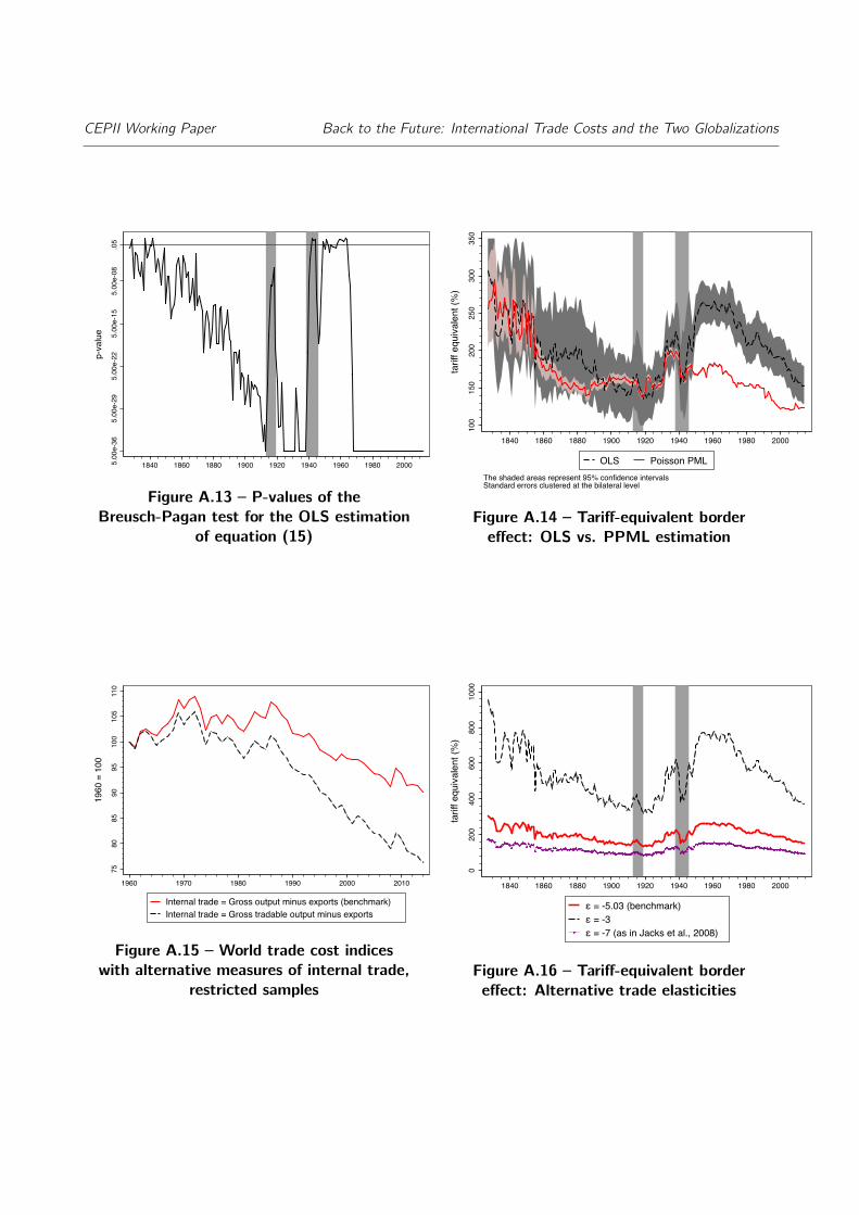
CEPII Working Paper Back to the Future: International Trade Costs and the Two Globalizations.05
5.00e-08
5.00e-15
5.00e-22
5.00e-29
5.00e-36
p-value
1840 1860 1880 1900 1920 1940 1960 1980 2000
Figure A.13 – P-values of theBreusch-Pagan test for the OLS estimation
of equation (15)
100
150
200
250
300
350
tarif
f equ
ivale
nt (%
)1840 1860 1880 1900 1920 1940 1960 1980 2000
OLS Poisson PMLThe shaded areas represent 95% confidence intervalsStandard errors clustered at the bilateral level
Figure A.14 – Tariff-equivalent bordereffect: OLS vs. PPML estimation
7580
8590
9510
010
511
0
1960
= 1
00
1960 1970 1980 1990 2000 2010
Internal trade = Gross output minus exports (benchmark)Internal trade = Gross tradable output minus exports
Figure A.15 – World trade cost indiceswith alternative measures of internal trade,
restricted samples
020
040
060
080
010
00
tarif
f equ
ival
ent (
%)
1840 1860 1880 1900 1920 1940 1960 1980 2000
ε = -5.03 (benchmark)ε = -3ε = -7 (as in Jacks et al., 2008)
Figure A.16 – Tariff-equivalent bordereffect: Alternative trade elasticities
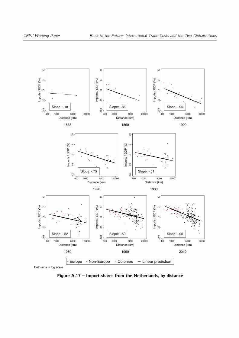
CEPII Working Paper Back to the Future: International Trade Costs and the Two Globalizations
Slope: -.18
.003
.03
.33
30Im
ports
/ G
DP
(%)
400 1000 5000 20000Distance (km)
1835
Slope: -.86
.003
.03
.33
30Im
ports
/ G
DP
(%)
400 1000 5000 20000Distance (km)
1860
Slope: -.95
.003
.03
.33
30Im
ports
/ G
DP
(%)
400 1000 5000 20000Distance (km)
1900
Europe Non-Europe Colonies Linear prediction
Slope: -.75
.003
.03
.33
30Im
ports
/ G
DP
(%)
400 1000 5000 20000Distance (km)
1920
Slope: -.51
.003
.03
.33
30Im
ports
/ G
DP
(%)
400 1000 5000 20000Distance (km)
1938
Europe Non-Europe Colonies Linear prediction
Slope: -.52
.003
.03
.33
30Im
ports
/ G
DP
(%)
400 1000 5000 20000Distance (km)
1950
Slope: -.59
.003
.03
.33
30Im
ports
/ G
DP
(%)
400 1000 5000 20000Distance (km)
1990
Slope: -.95
.003
.03
.33
30Im
ports
/ G
DP
(%)
400 1000 5000 20000Distance (km)
2010
Both axis in log scaleEurope Non-Europe Colonies Linear prediction
Figure A.17 – Import shares from the Netherlands, by distance