Trade and GDP Growth: Causal Relations in the United States and CanadaAuthor(s): George K. Zestos and Xiangnan TaoSource: Southern Economic Journal, Vol. 68, No. 4 (Apr., 2002), pp. 859-874Published by: Southern Economic AssociationStable URL: http://www.jstor.org/stable/1061496Accessed: 06/10/2010 18:22

Your use of the JSTOR archive indicates your acceptance of JSTOR's Terms and Conditions of Use, available athttp://www.jstor.org/page/info/about/policies/terms.jsp. JSTOR's Terms and Conditions of Use provides, in part, that unlessyou have obtained prior permission, you may not download an entire issue of a journal or multiple copies of articles, and youmay use content in the JSTOR archive only for your personal, non-commercial use.

Please contact the publisher regarding any further use of this work. Publisher contact information may be obtained athttp://www.jstor.org/action/showPublisher?publisherCode=sea.

Each copy of any part of a JSTOR transmission must contain the same copyright notice that appears on the screen or printedpage of such transmission.

JSTOR is a not-for-profit service that helps scholars, researchers, and students discover, use, and build upon a wide range ofcontent in a trusted digital archive. We use information technology and tools to increase productivity and facilitate new formsof scholarship. For more information about JSTOR, please contact support@jstor.org.

Southern Economic Association is collaborating with JSTOR to digitize, preserve and extend access toSouthern Economic Journal.

http://www.jstor.org

Southern Economic Journal 2002, 68(4), 859-874

Trade and GDP Growth: Causal

Relations in the United States and

Canada

George K. Zestos* and Xiangnan Taof

Causal relations between the growth rates of exports, imports, and the GDP of Canada and the United States are studied using the vector error correction (VEC) model. Utilizing time-series annual data (1948-1996), Granger causality tests are performed within the framework of the VEC model. Bidirectional causality is supported for Canada from the foreign sector to GDP and vice versa. A weaker relationship between the foreign sector and GDP is statistically supported for the United States. These results are also supported by comparing the total trade (exports plus imports) shares to GDP of the two neighboring economies. The Granger causality tests suggest that Canada is a more open economy than the United States and more trade dependent.

1. Introduction

Economic policies leading to economic growth and development have been studied by many economists for a long time. The literature in this area is rich; a number of candidate variables that may be related to economic growth have been considered and carefully examined. Some of these variables are investment, saving, inflation, inflation variability, governmental expenditures as a percentage of GDP, government deficit, and other mainly macroeconomic variables. Many economic models were constructed for the purpose of understanding economic

growth and to shed light on this issue.' A group of economists has focused exclusively on the

foreign sector, particularly on the relationship of exports, imports, and GDP growth. Emphasis on international trade dates back to the mercantilists more than two centuries ago. Mercantilists were firm believers that trade surpluses were the only favorable outcome for the domestic

economy from international trade relations. Mercantilists supported export promotion and pro-

* Department of Economics and Finance, Christopher Newport University, 1 University Place, Newport News, VA 23606, USA; E-mail gzestos@cnu.edu; corresponding author.

t Department of Management and Economics, Jiangnan University, Wuxi Jiangsu 214063, People's Republic of China; E-mail xntao@publicl.wx.js.cn.

We would like to thank an anonymous referee for exceptionally insightful and constructive comments. Similarly, we would like to express our gratitude to Professors Paul Serletis, Leo Michelis, Robert Winder, Michelle Vachris, and Nicholas Apergis for their helpful comments and suggestions. We are also grateful to the participants of the session where the paper was presented during the annual meetings of the Canadian Economic Association in Toronto, Ontario, Canada, May 29 to June 1, 1999. We also thank Mrs. Iris Price and Alexander Zestos for editing and typing the manuscript. Support for this research provided by a Faculty Development Grant from Christopher Newport University is gratefully acknowledged.

Received October 1998; accepted July 2001. A representative sample of these models is the work of Grier and Tullock (1989); Kormendi and Meguire (1985); Barro (1991); Mankiw, Romer, and Weil (1992); and Fischer (1993). Recently, endogenous growth models are becoming popular. A good example of this is Romer (1979, 1986).

859

860 George K. Zestos and Xiangnan Tao

tection of domestic industries since they were preoccupied with the accumulation of gold re- serves and not necessarily with the standards of living or the growth and economic development of the country per se. Many other authors, since the mercantilists, support the expansion of the

foreign sector for a variety of reasons. One of these reasons is that expansion of the export sector allows countries to attain economies of scale by specializing in production. This is par- ticularly important for smaller countries where the national markets are too small to allow

specialization. Some economists in favor of expansion of the export sector stress the common belief that the export sector is the most efficient sector of the economy. It is the sector where

workers enjoy the highest wages and firms earn the highest profits since only the most efficient

firms can compete successfully in the global market. Other supporters of export promotion point out that development of the export sector permits countries to have access to higher levels of

technology and technologically rich capital. This access is crucial to developing countries. Such

inflow of foreign capital and transfer of technology would not be possible without the export sector providing the means for payment since exports constitute the main source of foreign

exchange. Export expansion allows countries to follow a speedier pace toward industrialization

and economic growth. A variety of models have been suggested in the literature to study the effects of the foreign

sector on the domestic economy and vice versa. A group of econometric models rely on Granger

causality tests to explain relations between trade and the domestic economy. Three studies from

the literature that employed similar methodology are reviewed herein. Ahmad and Harnhirun

(1996) examined causality between exports and economic growth for five countries of the

Association of Southeast Asian Nations (ASEAN). The countries were Indonesia, Malaysia, the

Philippines, Singapore, and Thailand. Their model is a bivariate two-equation vector autore-

gression (VAR) covering the period 1966-1986. Ahmad and Harnhirum were able to test for

cointegration in only four of the countries since exports and GDP for Thailand were not inte-

grated in the same order. In the remaining four countries, they found that exports and GDP

were not cointegrated; consequently, the error correction term could not be included in their

model. Based on their results, Granger causality is supported from GDP to exports for each of

the four countries. This finding runs against the common belief that Southeast Asian countries

were exceptionally successful in achieving economic growth by following export promotion

policies. Dutt and Ghosh (1996) studied causality between exports and economic growth for a

relatively large sample of countries using the methodology of the error correction model (ECM). For the countries in which they found cointegration, the VEC model was estimated, and tests

for Granger causality were performed. Canada and the United States were two of the countries

in their sample, which covered the period 1953-1991. Dutt and Ghosh found no causality for

Canada between exports and GDP in either direction, but they found causality from GDP to

exports for the United States. In other countries the results were mixed. Some countries expe- rienced export-led growth, others the opposite (growth-led exports), some showed bidirectional

causality, and others demonstrated no causality. Their model differs from the present analysis since Dutt and Ghosh utilized a bivariate two-equation ECM model. An interesting feature of

the empirical part of this paper is that the authors pointed out the source of causality for each

country, that is, short- or long-run causality. This was based on the F- and t-tests, respectively. Restricted and unrestricted VAR models were employed by Ghartey (1993) to examine

any causal relation between exports and economic growth for Taiwan, Japan, and the United

States. Ghartey utilized Hsiao's version of Granger causality (Hsiao 1979). The three endoge-

Trade, GDP Growth in the U.S. and Canada

nous U.S. variables were GDP growth, export growth, and capital stock or the terms of trade

as the third variable. For the United States, it was found that economic growth causes export

growth, while the opposite is true for Taiwan. A feedback causal relationship or bidirectional

causality between exports and economic growth was found for Japan. It is clear from these and

other studies not reported here that there exists inconclusive evidence regarding the causal

relations of trade and GDP growth. Such inconclusiveness should be attributed partly to different

methodologies and periods covered by these studies as well as to genuine differences between

these economies. Similar results with the present study for Canada and the United States were

found in another study by Tao and Zestos (1999) for Japan and Korea. For Korea, a country that has a more trade-dependent economy than Japan, Granger causality tests indicate stronger causal relations.

This paper investigates causal relations between the growth of GDP, exports, and imports for Canada and the United States, using a trivariate VEC model. Evidence of cointegration for

both countries allowed us to estimate the VEC model. Granger causality tests were performed on the basis of the estimated VEC model. The model distinguishes two types of causality: long- run causality and short-run causality. The Granger causality tests reveal that the existence,

direction, and degree of Granger causality in the two countries differ substantially. These results

can be explained by historical differences of the two countries' economies. Stronger causal

relations were revealed in the growth of GDP, exports, and imports for Canada than for the

United States. These differences are attributed mainly to differing degrees of openness of the

two countries to the world economy. This paper is structured as follows. In section 2, we discuss international trade and devel-

opment theories. Granger causality tests, cointegration, and the VEC model are also presented in this section since they are the main tools of our analysis. In section 3, we describe and present

graphically the Canadian and the U.S. data and report the unit root tests for all variables. Since

the variables, exports, imports, and GDP were integrated of the same order and cointegrated, the model was estimated. The estimated VEC model is presented in section 4 together with the

results of the Granger causality tests. In section 5, a conclusion and a summary of the paper are given.

2. International Trade and Economic Development Theories

Many authors have stressed the positive effects of the export sector to the rest of the

economy, including Balassa (1978, 1985), Krueger (1980), Feder (1983), and Bhagwati and

Shrinivasan (1978). It has also been suggested that growth of output causes growth of exports

(Jung and Marshall 1985). Other groups of economists have opposed the export-led growth

approach. Nurkse (1961) advocated the "balanced growth" theory, while Prebisch (1962) sup-

ported the import substitution approach; the latter is diametrically opposite to the export-led

growth hypothesis. The import substitution approach dictates self-sufficiency of the country and

thus absolute trade protection. These trade and development theories have had an unparalleled influence on long-run economic policies adopted by countries. The two polar cases, export- oriented growth and import substitution, have split the developing countries into two distinct

groups. The first is represented mainly by the Southeast Asian countries and the second by the

Latin American countries. Economists have constructed many models for the sole purpose of explaining how trade

861

862 George K. Zestos and Xiangnan Tao

expansion contributes to economic growth. Estimation of a single equation and correlation

analysis dominated the early contributions. A few authors, such as Kwak (1994), adopted the factor growth accounting method, while other economists, such as Pack and Page (1994) and Esfahani (1991), utilized the neoclassical growth model. Some of these models employ cross- section multicountry data (see Afxentiou and Serletis 1991), while other models utilize time- series data for one country or a selected group of countries.

Granger Causality Models

Several econometric studies focus exclusively on Granger causality (Granger 1969). Grang- er causality from a variable X to a variable Y is established when knowledge of past values of X improve the prediction of future values of Y, over and above the prediction that is based on

knowledge of past values of Y alone.2 The simplest standard causality test is the pairwise Granger causality test. This is a bidi-

rectional test for Granger causality regarding only two variables. Granger causality from X to Y is established when the coefficients of the lagged differences of X are found to be jointly statistically significant and therefore help explain and predict Y, over and above what the lagged differences of Y can predict.

Another standard causality test similar to the pairwise Granger causality test is based on a model including more than one independent variable. The explicit format of this standard

causality model is constructed according to the empirical evidence of the stability properties of the time-series variables involved (see Serletis 1992); thus, if the variables are not cointegrated, the model must be expressed only in first differences. The null hypothesis is examined (F-test) to determine whether the coefficients of the lagged differences of an independent variable are

equal to zero in a single-equation model, including the lagged differences of the dependent variable and the lagged differences of at least another independent variable.

Cointegration and the ECM

Another causality test was developed by Engle and Granger (1987). In a bivariate setting, Engle and Granger introduced a new causality test while simultaneously introducing cointegra- tion. Generally stated, two variables are cointegrated if they have a common stochastic trend, that is, if they move together for a long period of time. More formally, two variables that are

stationary in their first differences but nonstationary in their levels are said to be cointegrated if there exists a stationary linear combination between them. To test for cointegration in the bivariate case, one has only to find statistical evidence that the residuals of a linear combination of the two variables are stationary. If cointegration is statistically established, this constitutes evidence that there exists a long-run equilibrium relationship between the two economic vari- ables.

For two cointegrated variables, according to Engle and Granger (1987), causality from X to Y can be established not only from finding jointly significant the coefficients of the

lagged differences of the variable X but also from finding significant the coefficient of the

one-period lagged error term of the cointegrating equation of the two variables. The idea is

This definition of Granger causality is different and weaker from what is usually meant by causality in general. Similarly, we can define causality from Y to X simply by reversing the two variables in the previous definition.

Trade, GDP Growth in the U.S. and Canada

rather simple: Since the variables are cointegrated, any equation describing a relation among them should include the one-period lagged stationary error term, 0,_1 (e.g., see Eqn. 5).

VEC Models

The error correction model described for the bivariate case can be generalized to include

many variables. A VEC model is a VAR model corrected by simply including the one-period

lagged error term (the cointegrating equation). The VEC models are based on the cointegration

theory (see Johansen 1991). A general VEC model is a system in n variables and n equations where each variable is a function of its own lagged differences, the lagged differences of the

other endogenous variables, and the error correction term. The number of cointegrating vectors

is called the cointegrating rank and cannot exceed n - 1.

There are a few versions of the cointegration model that can be estimated depending on the assumptions of the type of the cointegrating equation and the time plots of the time-

series variables.3 Once cointegration is established, the VEC model can be constructed. In

our case, it is a system of equations with the logarithmic first differences of each endogenous variable on the left-hand side of each equation. On the right-hand side are the lagged log- arithmic differences of all the endogenous variables and the one-period lagged error term

Ot-l_ The VEC model is presented in Equations 1 to 3 in first differences:

ALGDP, = aI + OLGDpA-t + C OliALGDPt_i + liALexportt_i i=1 i=1

k

+ 'liALimportti + elt (1) i=1

ALexportt = 32+ Lexp + Lett- + 2iALGDPt_i + 2iLexportt_i i=1 i=l

k

+ E y2iALimportti + E2t (2) i=1

r s

ALimport, = Y3 + LimportOt- + ciLGDPt_ + 3iALexportt_i i=l i=l

k

+ E y3iLimportt-i + 3t (3)

In this three-equation model, the three endogenous variables are the growth rate of the GDP

(ALGDP), the growth rate of exports (ALexport), and the growth rate of imports (ALimport).4 Each of the three variables is a function of the one-period lagged error correction term and the

3 EViews, the econometrics package used to carry out most of the empirical work, automatically estimates up to five different models; these include possible combinations of linear or quadratic trend for the time-series variables and linear trend in the cointegration equation in the presence or absence of an intercept.

4 The notation r,s,k refers to the optimum number of lagged differences included for each of the three endogenous variables.

863

864 George K. Zestos and Xiangnan Tao

lagged logarithmic differences of the other two dependent variables.5 Each equation also in- cludes a random error term E.

The three coefficients of the error correction term, aLGDP, PLexport, and YLimport, are often referred to as speed-of-adjustment parameters. They reflect the response with which the

system of the cointegrated variables GDP, exports, and imports move back to their long-run equilibrium relation. The larger the three coefficients of the error correction term, Ot,_, the

greater the response of the cointegrated variables to move back to their long-run equilibrium relation. Thus, the three coefficients capture the effect of the deviation of the variables from their long-run equilibrium on the rate of growth of each left-hand-side variable.

The estimation of the model allows testing for Granger causality. Particularly, each

equation can be tested to determine whether any of the two right-hand-side variables cause the left-hand-side variable. The null hypothesis of noncausality can be rejected not only if one finds significant the lagged logarithmic differences (F-test) of a particular variable in

any of the three equations but also if one finds significant the coefficient of the lagged error correction term 0t,_ (t-test).

3. Data

A data set of the real variables, exports, imports, and GDP was constructed for each

country consisting of 49 observations (1948-1996). In Figure 1, real exports, real imports, and total trade (the sum of real exports and real imports) are presented each as a percentage of real GDP. The three trade variables (ratios) of both countries have been increasing during the entire sample period. As can be seen from Figure 1, there is a substantial difference between the Canadian and the U.S. trade data. According to the graphs in Figure 1, Canada was always a more open economy than the United States. For example, in the last year of the sample (1996), total trade as a percentage of GDP for Canada was approximately 80%; this is much higher than the corresponding U.S. total-trade-to-GDP ratio, which was ap- proximately 25%.6

We chose to employ annual instead of quarterly data since we believe that Granger causality is a timely phenomenon and that the interaction of economic variables cannot work in short

periods of a few quarters. In fact, it takes years for the complete interaction effects to materialize. For this reason, we are in agreement with Dutt and Ghosh (1996), who also utilize annual instead of quarterly data.

Stability Properties of the Variables

When formulating models with time-series variables, one must be concerned with the

stability properties of the variables. According to Phillips (1987), for a set of variables found to be integrated of order one or I(1) but not cointegrated, any regression involving the levels of these variables is spurious. This implies that only cointegrated variables can be used in a

5 It is possible to find more than one cointegrating vector; then equal numbers of error correction terms have to be included in the VEC model.

6 All data are from the International Financial Statistics of the International Monetary Fund (IMF), the CD-ROM database. We transformed nominal exports and imports to real by dividing by the export and import price indices; all real variables are expressed in 1990 national currency units. In this study, we use only real data.

Trade, GDP Growth in the U.S. and Canada

Real Canadian Exports, Imports, and Total Trade Over GDP

1954 1960 1966 1972 1978 1984 1990 1996

Real U.S. Exports, Imports, and Total Trade Owr GDP

30

- Exp&Imp/GDP

25 - - Exports/GDP

-- Imports/GDP

20 -

15 -

0

10 -

I I I I I I I I I I19 I78I i t I } t I I I

1948 1954 1960 1966 1972 1978

Figure 1. Real Canadian and U.S. Exports, Imports, and Total Trade over GDP.

1984 1990 1996

model that is expressed in levels of the variables. However, if the variables are not cointegrated,

any model involving these variables should be stated in their first differences.

All variables used in this study are the logarithms of the original data. We performed unit

root tests and cointegration for all variables. The three variables-GDP, exports, and imports-

865

90

80

70

60

o

= 50

0 t 40

30

20

10

0 t

1948

866 George K. Zestos and Xiangnan Tao

Table 1. Unit Root Testsa

ADF Test Phillips-Perron Test

Trend and Trend and Constant Constant Constant Constant

T~~~~~Level Canadian Data Level

Lexport -3.502* [1] -0.012 [1] -2.906 0.710 Limport -3.288* [1] -0.520 [1] -2.782 -0.393 LGDP -0.320 [1] -2.835* [1] 0.022 -3.288**

First difference

Alexport -4.671*** [1] -4.627*** [1] -4.317*** -4.397*** Alimport -5.403*** [1] -5.466*** [1] -5.689*** -5.759*** ALGDP -5.298*** [2] -4.188*** [1] -6.114*** -5.098***

U.S.Data Level Lexport -3.135 [3] 0.016 [4] -3.364* 0.735 Limport -2.786 [1] -0.811 [1] -2.588 -0.383 LGDP -2.970 [1] -1.568 [3] -1.936 -2.171

First difference

Alexport -3.862*** [3] -3.951*** [3] -6.676*** -6.669*** Alimport -5.167*** [1] -5.227*** [1] -6.793*** -6.843*** ALGDP -5.296*** [2] -5.106 [2] [2] -6.026*** -5.561***

a The figures in brackets denote the number of lags that were selected by the Schwarz Information Criterion (SIC). * Significant at the 10% confidence level.

** Significant at the 5% confidence level. *** Significant at the 1% confidence level.

were found to be I(1) and cointegrated; consequently, a VEC model was formulated and esti- mated. Causality tests were performed on the basis of the estimated VEC model.

Unit Root Tests

Table 1 reports the empirical results of the unit root tests for the real Canadian and U.S. data. The augmented Dickey-Fuller (ADF) and the Phillips-Perron (1988) tests were

performed. Two versions of both tests were performed, that is, with a constant only and with a constant and trend. The Phillips-Perron test is robust in the presence of both serial correlation and time-dependent heteroscedasticity. To further enhance the quality of the results in the ADF test, we included a number of lagged differences according to the Schwarz Information Criterion (SIC; Schwarz 1978). Inclusion of the optimum number of

lagged differences ensures that the error becomes approximately white noise. The regression equation for the ADF test is as follows:

n AXt = 30 + 1lt + P32Xt-_ + E ()iAXt-i + et

i=1 (4)

where et is the regression error assumed to be stationary with zero mean and a constant variance. A unit root test is a significance test on the coefficient of X,_ . This is performed using the MacKinnon (1991) critical values and not the standard t-table since the left-hand-side variable under the null hypothesis is nonstationary. The Phillips-Perron test is based on the same re-

gression as the ADF test but without the lagged differences. The t-statistic of the 32 coefficient

Trade, GDP Growth in the U.S. and Canada

Table 2. Cointegration Results of Canadian Data

1% Critical 1% Critical Ho: Rank = r Eigenvalue hmax Values Atrace Values

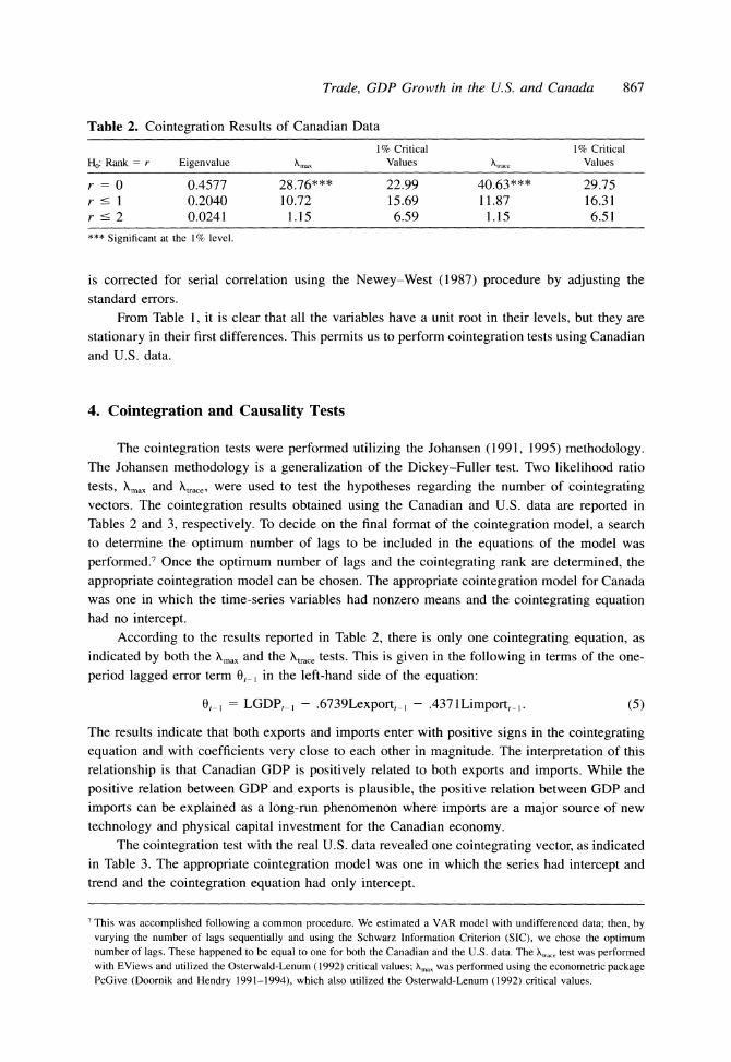
r = 0 0.4577 28.76*** 22.99 40.63*** 29.75 r < 1 0.2040 10.72 15.69 11.87 16.31 r < 2 0.0241 1.15 6.59 1.15 6.51 *** Significant at the 1% level.

is corrected for serial correlation using the Newey-West (1987) procedure by adjusting the

standard errors. From Table 1, it is clear that all the variables have a unit root in their levels, but they are

stationary in their first differences. This permits us to perform cointegration tests using Canadian

and U.S. data.

4. Cointegration and Causality Tests

The cointegration tests were performed utilizing the Johansen (1991, 1995) methodology. The Johansen methodology is a generalization of the Dickey-Fuller test. Two likelihood ratio

tests, Xmax and trace, were used to test the hypotheses regarding the number of cointegrating vectors. The cointegration results obtained using the Canadian and U.S. data are reported in Tables 2 and 3, respectively. To decide on the final format of the cointegration model, a search to determine the optimum number of lags to be included in the equations of the model was

performed.7 Once the optimum number of lags and the cointegrating rank are determined, the

appropriate cointegration model can be chosen. The appropriate cointegration model for Canada was one in which the time-series variables had nonzero means and the cointegrating equation had no intercept.

According to the results reported in Table 2, there is only one cointegrating equation, as indicated by both the K\max and the Xtrace tests. This is given in the following in terms of the one-

period lagged error term 0,_, in the left-hand side of the equation:

0,_l = LGDP,_l - .6739Lexport,_, - .4371Limport,_ . (5)

The results indicate that both exports and imports enter with positive signs in the cointegrating equation and with coefficients very close to each other in magnitude. The interpretation of this

relationship is that Canadian GDP is positively related to both exports and imports. While the

positive relation between GDP and exports is plausible, the positive relation between GDP and

imports can be explained as a long-run phenomenon where imports are a major source of new

technology and physical capital investment for the Canadian economy. The cointegration test with the real U.S. data revealed one cointegrating vector, as indicated

in Table 3. The appropriate cointegration model was one in which the series had intercept and trend and the cointegration equation had only intercept.

7 This was accomplished following a common procedure. We estimated a VAR model with undifferenced data; then, by varying the number of lags sequentially and using the Schwarz Information Criterion (SIC), we chose the optimum number of lags. These happened to be equal to one for both the Canadian and the U.S. data. The Xtrac, test was performed with EViews and utilized the Osterwald-Lenum (1992) critical values; Xmax was performed using the econometric package PcGive (Doornik and Hendry 1991-1994), which also utilized the Osterwald-Lenum (1992) critical values.

867

868 George K. Zestos and Xiangnan Tao

Table 3. Cointegration Results for U. S. Data

5% Critical 5% Critical Ho: Rank = r Eigenvalue Xmax Values htrace Values

r = 0 .3760 22.17** 21.17 35.51** 29.69 r < 1 .2441 13.15 14.1 13.35 15.41 r - 2 .0041 .19 3.8 .19 3.76 ** Significant at the 5% level.

The cointegrating equation is presented in Equation 6, with the one-period lagged error

term 0,_i in the left-hand side of the equation:

o,_t = LGDP,_ -.851Lexport,_I + .3750Limport,_I - 5.6699. (6)

For the U.S. data, exports and GDP are positively related, whereas imports and GDP are neg-

atively related. Comparing these results with those obtained for Canada reveals a major differ-

ence, as imports in the United States do not play a positive role in explaining GDP. A possible

explanation for this is that the United States has been a major industrial country for the period covered by our sample and was not relying on imported technology and physical capital.

According to Granger (1988), causality within the framework of the VEC model can occur

in two different ways. The first way is through the impact of the lagged differences of a right- hand-side variable. The second way is through the error correction term, which is a function of

the one-period lagged values of the variables. Granger suggested that the impact of the lagged differences of a right-hand-side variable on the left-hand-side variable captures the short-run

dynamics of the system and therefore can be interpreted as short-run causality. The impact of

the one-period lagged error correction term on the left-hand-side variable captures the extent

that the variables are out of equilibrium; thus, it can be interpreted as long-run causality.8 Toda

and Phillips (1994), who discuss the asymptotics for causality tests with a VEC model, distin-

guish the two parts of the hypothesis as "short-run noncausality" and "long-run noncausality." We reproduce the VEC model in Equations 1'-3' without the summation sign before the

right-hand-side variables since the optimum number of lagged differences for all variables was

found to equal one. Such presentation of the model will facilitate the understanding of the

Granger causality tests:

ALGDP, = oa + (LGDPOt_- + Ox,lALGDP,_ + P311ALexport, + y,,ALimport,_, + el, (1)'

Lexport, = expoexrtO, P P t-l + a2iALGDPt_, + 321ALexportt_, + Y21ALimport,_t + E2t (2)'

ALimport,= y 3 + 'YLimportOt-I + ot31ALGDP,t- + 331ALexport,_t + y31ALimport, _ + e3t (3)'

In terms of our model, the null hypothesis of short-run noncausality, based on Equation 1' from exports to GDP, is stated as 3P, = 0. Similarly from Equation 1', the null hypothesis of short-run noncausality from imports to GDP is stated by setting y/Y = 0. The null hypothesis for long-run noncausality is stated by setting each coefficient, OLLGDP, 3Lexpoor or Limport

= 0,

separately in each equation.9

8 This division of the two sources of causality is not totally settled in the literature, unless the decomposition of the

frequency of the error correction term is studied carefully (see Granger 1988). See also Jones and Joulfaian (1991) on this issue, who also distinguish between short-run and long-run Granger causality.

9 At least one of the three coefficients must be significantly different than zero to support long-run causality.

Trade, GDP Growth in the U.S. and Canada 869

Interestingly, standard asymptotics apply here for purposes of hypothesis testing. Since the

variables exports, imports, and GDP growth are cointegrated, their error correction term is a

stationary variable with zero mean. According to Sims, Stock, and Watson (1990), the t-ratio of the coefficient of the error correction term follows an asymptotic standard normal distribution.

Similarly, since each variable was found to be I(1), each lagged difference is a stationary variable, and testing their joint significance can be accomplished using a standard F-test.

A test for overall Granger causality that combines the two sources of causality was also constructed. If the coefficients of the error correction term and the coefficients of the lagged differences of a right-hand-side variable are jointly significant, Granger causality is established. The null hypothesis of Granger noncausality in our model from exports to GDP based on

Equation 1' can be stated as OLGDP = 1 = 0. On the other hand, the null hypothesis of Granger noncausality from imports to GDP can be stated as OtLGDP = I1I = 0. The appropriate test is an F (Wald)-test.10 Since this test considers both sources of causality, it is the only test reported by some authors to test for Granger causality, especially when these authors are not interested in the long- and short-run impacts of the variables.

The Estimated VEC Model and Causality Tests with Canadian and U.S. Data

Since it was found that the Canadian and U.S. variables were cointegrated, this suggested that the VEC model of Equations 1'-3' is valid and can be estimated. The estimated model is

presented in Tables 4 and 5. Three causality tests are reported in Tables 4 and 5. The first test is a t-test on the coefficient

of the error correction term 0,_I; this is a test for long-run noncausality. The second test is an F-test for short-run noncausality. In our model, this turns out to be a t-test as well, but since the two tests are equivalent, we report only the F-test. The third test is a joint F-test on the coefficients of the error correction term and the lagged differences of each relevant right-hand- side variable in each equation. The calculated values of the joint F-statistic are reported under the columns F, and F2 since two such tests must be performed in each equation. In Equation 1', for instance, we test the null hypothesis OLGDP = P1 = 0 using F, and the null hypothesis OLLGDP = '11 = 0 using F2. In the first hypothesis we test whether exports Granger cause GDP, while in the second we test whether imports Granger cause GDP Similar interpretations apply for F, and F2 in each of the other two equations."

From the estimated VEC model in Table 4 for the Canadian data, one observes that the

lagged error term 0,_i is significant in all three equations. This finding alone implies long-run causality from the right-hand-side variables to the three left-hand-side variables, but it alone cannot reveal the exact direction of the causality. From Equation 7, it is uncertain whether

causality is implied from exports or imports to GDP, according to the F-test on the lagged logarithmic difference of exports and imports, respectively. According to the joint F-test for

Granger causality, however, each right-hand-side variable, exports and imports, separately

10 The ratio [(RSS, - RSS,)/j + 1]/(RSS,/T - r - s - k - 2), where j = r,s,k has an asymptotic F-distribution with j + 1 and T- r -s -k -2 degrees of freedom, j is an index taking values equal to the number of lags of the right- hand-side variable, s, r, and k, where RSS, = unrestricted residual sum of squares, RSS, = restricted residual sum of squares, and r, s, and k = number of included lags for GDP, exports, and imports. From Equation 2', we test the null hypothesis PLexport

= O21 = 0 using F1 and the null hypothesis 3Lexport =

Y21 = 0. The first hypothesis tests whether GDP Granger causes exports, while in the second we test the hypothesis of whether imports Granger cause exports. Similarly from Equation 3', we test the null hypothesis of whether GDP causes imports and the null hypothesis of whether exports cause imports.

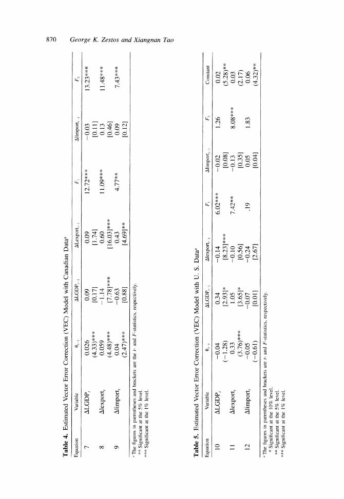
Table 4. Estimated Vector Error Correction (VEC) Model with Canadian Dataa

Equation Variable 0,_, ALGDP,_ ALexport,_ F, Alimport, i F,

7 ALGDP, 0.026 0.09 0.09 12.72*** -0.03 13.23*** (4.33)*** [0.17] [1.74] [0.11]

8 Alexport, 0.059 -1.14 0.60 11.09*** 0.13 11.48*** (4.48)*** [7.78]*** [16.03]*** [0.46]

9 Alimportt 0.04 -0.63 0.43 4.77** 0.09 7.43*** (2.47)*** [0.88] [4.69]** [0.12]

a The figures in parentheses and brackets are the t- and F-statistics, respectively. ** Significant at the 5% level.

*** Significant at the 1% level.

Table 5. Estimated Vector Error Correction (VEC) Model with U. S. Dataa

Equation Variable 0,t~ ALGDP,_ Alexport,_ F, Alimport,_ ] F2 Constant

10 ALGDP, -0.04 0.34 -0.14 6.02*** -0.02 1.26 0.02 (-1.28) [2.93]* [8.23]*** [0.08] (5.28)**

11 Alexport, 0.33 1.05 -0.10 7.42** -0.13 8.08*** 0.03 (3.76)*** [3.65]* [0.56] [0.35] (2.17)

12 Alimport, -0.05 -0.07 -0.24 .19 0.05 1.83 0.06 (-0.61) [0.011 [2.67] [0.04] (4.32)**

a The figures in parentheses and brackets are t- and F-statistics, respectively. * Significant at the 10% level.

** Significant at the 5% level. *** Significant at the 1% level.

Q CZ o

.t

c3

$

Ch h

I"Z a~

Trade, GDP Growth in the U.S. and Canada

Granger causes GDP. Equation 8 indicates inverse causality from GDP to exports. Imports were

found not to cause exports according to the F-test on the lagged logarithmic difference of

imports. The joint F-tests for Granger causality, however, suggest that GDP and imports each

separately Granger cause exports. Finally, Equation 9 indicates that exports Granger cause im-

ports, but GDP does not Granger cause imports, according to the F-test on the lagged differences

of each of these variables separately. The joint F-test for Granger causality suggests that both

GDP and exports each separately cause imports at the 5% and 1% levels of significance, re-

spectively. We interpret these results as a strong case of causality in a complete circle from the

domestic growth of the Canadian economy to the foreign sector and vice versa. Export expan- sion secured the necessary foreign exchange to pay for Canadian imports, which facilitated

domestic economic growth. It is very likely that the original exports were mainly from the

primary sector, that is, agricultural commodities, lumber, minerals, and so on, since Canada has

always been a country rich in natural resources. On the other hand, Canadian imports were

manufacturing products, either final consumer goods or tools and machinery, which contributed to industrialization and growth of the domestic economy. This process gradually transformed the Canadian economy with imports playing a favorable role in domestic growth. The latter

point is supported by the positive relationship in the cointegrating vector between GDP growth and the growth of imports and by the historical trade data of exports, imports, and total trade, which amounted to a large and increasing percentage of Canadian GDP during the entire sample period (Figure 1).

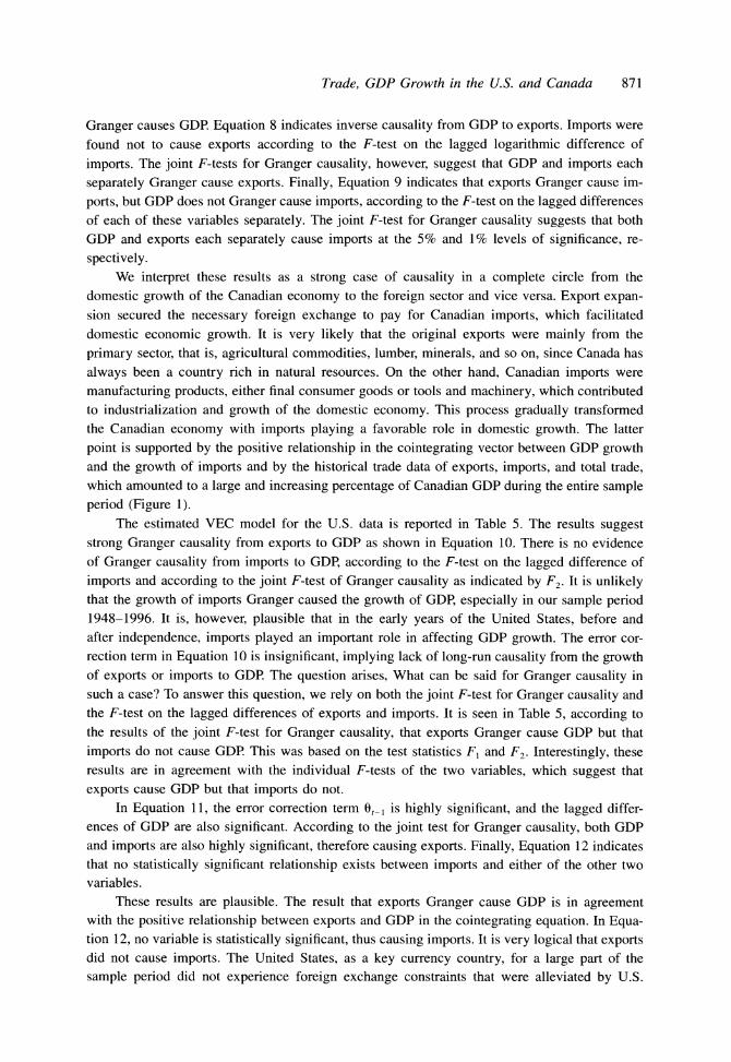
The estimated VEC model for the U.S. data is reported in Table 5. The results suggest strong Granger causality from exports to GDP as shown in Equation 10. There is no evidence of Granger causality from imports to GDP, according to the F-test on the lagged difference of

imports and according to the joint F-test of Granger causality as indicated by F2. It is unlikely that the growth of imports Granger caused the growth of GDP, especially in our sample period 1948-1996. It is, however, plausible that in the early years of the United States, before and after independence, imports played an important role in affecting GDP growth. The error cor- rection term in Equation 10 is insignificant, implying lack of long-run causality from the growth of exports or imports to GDP. The question arises, What can be said for Granger causality in such a case? To answer this question, we rely on both the joint F-test for Granger causality and the F-test on the lagged differences of exports and imports. It is seen in Table 5, according to the results of the joint F-test for Granger causality, that exports Granger cause GDP but that

imports do not cause GDP. This was based on the test statistics F, and F2. Interestingly, these results are in agreement with the individual F-tests of the two variables, which suggest that

exports cause GDP but that imports do not. In Equation 11, the error correction term 0 t_ is highly significant, and the lagged differ-

ences of GDP are also significant. According to the joint test for Granger causality, both GDP and imports are also highly significant, therefore causing exports. Finally, Equation 12 indicates that no statistically significant relationship exists between imports and either of the other two variables.

These results are plausible. The result that exports Granger cause GDP is in agreement with the positive relationship between exports and GDP in the cointegrating equation. In Equa- tion 12, no variable is statistically significant, thus causing imports. It is very logical that exports did not cause imports. The United States, as a key currency country, for a large part of the

sample period did not experience foreign exchange constraints that were alleviated by U.S.

871

872 George K. Zestos and Xiangnan Tao

exports. The U.S. dollar was, and still is, a widely accepted currency for international payments. These results are congruent with the joint F-test, which also indicated that no other variable causes imports, and the growth of imports did not cause GDP growth as shown in Equation 10. In Equations 10 and 12, the significance of the constant terms implies that there are possible omitted variables in the model. For example, in Equations 10 and 12, the U.S. capital account

surplus may be an omitted variable that caused both growth of GDP and growth of imports. We included the real U.S. capital account surplus in lieu of U.S. imports in the VEC model and estimated this model for the period 1960-1966. We found that U.S. capital account surplus does not Granger cause, or is caused by, U.S. GDP or exports.'2

The interpretation of the two sources of causality is meaningful. In Canada, a country very much dependent on trade, the growth of exports, imports, and GDP is in a long-run equilibrium relationship, as indicated by a highly significant cointegrating equation and error correction term in all three equations. According to the joint F-test for Granger causality, every right-hand-side variable was also significant. For the United States, we found a weaker relation between foreign trade and growth of the domestic economy. The cointegrating equation was significant at the

5% level. The error correction term was significant in only one of the three equations of the

VEC model, and only one right-hand-side variable was highly significant in both Equations 10

and 11.

5. Conclusion

On the basis of a VEC trivariate model, which includes the growth variables of GDP,

exports, and imports, Granger causality tests were performed to reveal possible directions of

causality. The VEC model was estimated for the period 1948-1996 for Canada and the United

States. The results for Canada show that the three variables are closely related and that causality is established in every possible direction. For the United States, exports were found to cause

GDP. Comparing the Canadian and U.S. Granger causality tests, strong causality is supported for Canada, but not an equally strong relation is supported for the United States. This is con-

sistent with the fact that Canada is more trade dependent and has a more open economy than

the United States. This is clearly indicated in Figure 1, where the exports, imports, and trade

shares of the two neighboring countries are presented. Three explanations are provided for the weaker case of Granger causality in the United

States. First, the United States is a large industrial country with a large national market that

has been in some ways in the past economically isolated from the rest of the world. Second, the United States, as a key currency country for a long period, was able to import goods and

services and invest in foreign countries regardless of the level of its exports. As a result, exports and imports in the United States were not closely related. In other countries, exports provide the required foreign exchange to pay for their imports. Third, prolonged U.S. government def-

icits since the early 1980s resulted in high U.S. interest rates, which attracted foreign financial

capital in the United States. The exceptionally large U.S. capital surplus has most likely distorted the long-run relationship between U.S. exports, imports, and GDP.

12 It was not possible to find data for the entire 1948-1996 sample for the U.S. capital account surplus. A smaller data set for 1960-1996, however, was constructed for the U.S. real capital account surplus in constant 1990 dollars from the Economic Report of the President (1999).

Trade, GDP Growth in the U.S. and Canada 873

References

Afxentiou, Panayiotis C., and Apostolos Serletis. 1991. Exports and GNP causality in the industrial countries: 1950- 1985. Kyklos 44(Fasc. 2):167-79.

Ahmad, Jaleel, and Somchai Harnhirun. 1996. Cointegration and causality between exports and economic growth: Evi- dence from the ASEAN countries. Canadian Journal of Economics 29:S413-6.

Balassa, Bela. 1978. Export and economic growth: Further evidence. Journal of Development Economics 5:181-9. Balassa, Bela. 1985. Exports, policy choices, and economic growth in developing countries after the 1973 oil shock.

Journal of Development Economics 18:23-35. Barro, Robert J. 1991. Economic growth in a cross section of countries. Quarterly Journal of Economics 106:407-43.

Bhagwati, Jagdish N., and T N. Shrinivasan. 1978. Trade policy and development. In International economic policy: Theory and evidence, edited by Rudiger Dorbusch and Jacob A. Frenkel. Baltimore: The Johns Hopkins Uni- versity Press, pp. 1-38.

Doornik, J. A., and D. E Hendry. 1991-1994. Interactive econometric modeling of dynamic systems. London: Interna- tional Thomson Publishing.

Dutt, Swarna D., and Dipak Ghosh. 1996. The export growth-Economic growth nexus: A causality analysis. Journal

of Developing Areas 30:167-82. Council of Economic Advisors. 1999. Economic report of the President, February 1999. Washington, DC: Government

Printing Office.

Engle, Robert F, and Clive W. Granger. 1987. Cointegration and error correction: Representation, estimation and testing. Econometrica 55:251-76.

Esfahani, Hadi Salehi. 1991. Exports, imports, and economic growth in semi-industrialized countries. Journal of Devel- opment Economics 35:93-116.

Feder, Gershon. 1983. On exports and economic growth. Journal of Development Economics 12:59-73. Fischer, Stanley. 1993. The role of macroeconomic factors in growth. Journal of Monetary Economics 32:485-512. Ghartey, Edward E. 1993. Causal relationship between exports and economic growth: Some empirical evidence in Taiwan,

Japan and the U.S. Applied Economics 25:1145-52. Granger, C. W. J. 1969. Investigating causal relations by econometric models and cross-spectral methods. Econometrica

37:424-38. Granger, C. W. J. 1988. Some recent developments in a concept of causality. Journal of Econometrics 39:199-211. Grier, Kevin B., and Gordon Tullock. 1989. An empirical analysis of cross-national economic growth, 1951-80. Journal

of Monetary Economics 24:259-76. Hsiao, Cheng. 1979. Autoregressive modeling of Canadian money and income data. Journal of the American Statistical

Association 74:553-60. Johansen, Soren. 1991. Estimation and hypothesis testing of cointegration vectors in Gaussian vector autoregressive

models. Econometrica 59:1551-80. Johansen, Soren. 1995. Likelihood-based inference in cointegrated vector autoregressive models. Oxford: Oxford Uni-

versity Press. Jones, J. D., and David Joulfaian. 1991. Federal government expenditures and revenues in the early years of the American

republic: Evidence from 1792 to 1860. Journal of Macroeconomics 13:133-55. Jung, Woo S., and Peyton J. Marshall. 1985. Exports, growth and causality in developing countries. Journal of Devel-

opment Economics 18:1-12. Kormendi, Roger C., and Philip G. Meguire. 1985. Macroeconomic determinants of growth: Cross country evidence.

Journal of Monetary Economics 16:141-63.

Krueger, Anne 0. 1980. Trade policy as an input to development. American Economic Review 70:288-92. Kwak, Hyuntai. 1994. Changing trade policy and its impact on TFP in the Republic of Korea. The Developing Economies

32(4):398-422. MacKinnon, James G. 1991. Critical values for cointegration tests. In Long-run economic relationships: Readings in

cointegration, edited by Robert F Engle and Clive W. J. Granger. Oxford: Oxford University Press, pp. 267-76. Mankiw, N. Gregory, David Romer, and David N. Weil. 1992. A contribution to the empirics of economic growth.

Quarterly Journal of Economics 107:407-38. Newey, Whitney K., and Kenneth D. West. 1987. A simple positive semi-definite heteroskedasticity and autocorrelation

consistent covariance matrix. Econometrica 55:703-8. Nurkse, R. 1961. Trade theory and development policy. In Economic development of Latin America, edited by H. S.

Ellis. New York: St. Martin Press, pp. 236-45. Osterwald-Lenum, Michael. 1992. A note with quantiles of the asymptotic distribution of the maximum likelihood

cointegration rank test statistics. Oxford Bulletin of Economics and Statistics 54:461-72. Pack, Howard, and John M. Page, Jr. 1994. Accumulation, exports, and growth in the high performing Asian economies.

Carnegie-Rochester Conference Series on Public Policy 40(June):199-236.

874 George K. Zestos and Xiangnan Tao

Phillips, P C. B. 1987. Time series regression with a unit root. Econometrica 55:277-301.

Phillips, P. C. B., and P Perron. 1988. Testing for a unit root in time series regression. Biometrika 75:335-46. Prebisch, R. 1962. Economic development of Latin America and its principal problems. Economic Bulletin for Latin

America 7:1-21.

Romer, P M. 1979. Capital accumulation and long-run growth. In Modern business cycle theory, edited by R. J. Barro.

Cambridge, MA: Harvard University Press, pp. 51-127. Romer, P. M. 1986. Increasing returns and long run growth. Journal of Political Economy 94:1002-37. Schwarz, A. 1978. Estimating the dimension of a model. Annals of Statistics 6:461-4. Serletis, Apostolos. 1992. Export growth and Canadian economic development. Journal of Development Economics 38:

133-45. Sims, C. A., J. H. Stock, and M. W. Watson. 1990. Inference in linear time series models with some unit roots. Econo-

metrica 58:113-44. Tao, Xiangnan, and George Zestos. 1999. Sources of economic growth in Japan and Korea: Causality tests. Journal of

International Economic Studies, no. 13:117-32. Toda, Hiro Y., and Peter C. B. Phillips. 1994. Vector autoregression and causality: A theoretic overview and simulation

study. Econometric Reviews 13:259-85.