Tracking of Multiple Moving Sources Using Recursive EM...

Tracking of Multiple Moving Sources Using Recursive

EM Algorithm

Pei–Jung Chung∗, Johann F. Bohme∗∗, Alfred O. Hero∗

∗ Dept. of Electrical Engineering and Computer Science, University of Michigan, Ann Arbor, USA

∗∗ Signal Theory Group, Dept. of Electrical Engineering and Information Science

Ruhr-Universitat Bochum, D–44780 Bochum, Germany

Email: peijung [email protected], [email protected], [email protected]

Abstract

This work deals with recursive direction of arrival (DOA) estimation of multiple moving

sources. Based on the recursive EM algorithm, we develop two recursive procedures to esti-

mate the time-varying DOA parameter for narrow band signals. The first procedure requires

no prior knowledge about the source movement. The second procedure assumes that the

motion of moving sources is described by a linear polynomial model. The proposed recursion

updates the polynomial coefficients when a new data arrives. The suggested approaches have

two major advantages: simple implementation and easy extension to wideband signals. Nu-

merical experiments show that both procedures provide excellent results in a slowly changing

environment. When the DOA parameter changes fast or two source directions cross with

each other, the procedure designed for a linear polynomial model has a better performance

than the general procedure. Compared to the beamforming technique [17] based on the

same parameterization, our approach is computationally favorable and has a wider range of

applications.

1

1 Introduction

The problem of estimating direction of arrival (DOA) of plane waves impinging on a sensor array

is of fundamental importance in many applications such as radar, sonar, geophysics and wireless

communication. The maximum likelihood (ML) method is known to have excellent statistical

performance and is robust against coherent signals and small sample numbers [2]. However, the

high computational cost associated with ML method makes it less attractive in practice.

To improve the computational efficiency of the ML approach, numerical methods such as

the expectation and maximization (EM) algorithm [11] was suggested in [12] [5][16]. Recursive

procedures based on the recursive EM algorithm for estimating constant DOA parameters were

discussed in [6] [15]. Similar procedures for tracking multiple moving sources were studied in [8]

[13]. In [13], the authors focused on narrow band sources and assumed known signal waveforms.

The recursive EM algorithm is a stochastic approximation procedure for finding ML estimates.

It was first suggested by Titterington [18] and extended to the multi-dimensional case in [6]. As

it was pointed out by Titterington, recursive EM can be seen as a sequential approximation of

the EM algorithm. The gain matrix of recursive EM is the inversion of the augmented data

information matrix. Through proper design of the augmentation scheme, the augmented data

and the corresponding information matrix usually have a simple structure [11]. In this case, the

recursive EM algorithm is very easy to implement. For constant parameter, estimates generated

by recursive EM are strongly consistent and asymptotically normally distributed. For time-

varying parameter, the tracking ability of a stochastic approximation procedure depends mainly

on the dynamics of the true parameter, gain matrix and step size [1].

Based on recursive EM, we shall derive two recursive procedures for estimating time-varying

DOA. The first procedure does not require any prior knowledge on the motion model. The only

assumption is that the unknown parameter changes slowly with time. The second procedure

assumes that the time-varying DOA parameter θ(t) is described by a linear polynomial of time.

This model is important since a smooth function θ(t) can be approximated by a local linear

polynomial in a short time interval [17]. The procedure reported in [8] employs a decreasing

step size to estimate the polynomial coefficients. However, since the DOA parameter θ(t) and

the log-likelihood function change with time, a decreasing step size may not capture the non-

stationary feature of the underlying system over a long period. To overcome this problem, we

suggest a constant step size to be used in the algorithm. It is noteworthy that both procedures

2

are aimed at maximizing the expected concentrated likelihood function [9]. Introducing a linear

polynomial model implies increasing the dimension of the parameter space. With the additional

degree of freedom, the procedure designed for a linear polynomial model should perform better

than the general one.

In contrast to methods based on subspace tracking [22] or two dimensional beamforming

[17], our approach can be easily generalized to wideband cases including underwater acoustic

signals. Unlike the Kalman type algorithms [23], recursive procedures considered here have a

much simpler implementation.

This paper is outlined as follows. We describe the signal model and the recursive EM algo-

rithm briefly in section 2 and section 3. Section 4 presents two recursive procedures for localizing

moving sources. Simulation results are discussed in section 5. We give concluding remarks in

section 6.

2 Problem Formulation

Consider an array of N sensors receiving M far field waves from unknown time-varying directions

θ(t) = [θ1(t) . . . θM (t)]. The array output x(t) ∈ CN×1 at time instant t is expressed as

x(t) = H(θ(t))s(t) + u(t), t = 1, 2, . . . (1)

where the steering matrix

H(θ(t)) = [ d(θ1(t)) . . . d(θM (t)) ] ∈ CN×M (2)

consists of M steering vectors d(θm(t)) ∈ CN×1, (m = 1, . . . ,M). To avoid ambiguity, we assume

M < N . The signal waveform s(t) = [s1(t) . . . sM (t)]T ∈ CM×1 is considered as unknown and

deterministic. (·)T denotes the transpose of a vector. Furthermore, the noise process u(t) ∈ CN×1

is independent identically complex normally distributed with zero mean and covariance matrix

νI, where ν represents the unknown noise spectral parameter and I is the identity matrix.

In the following, we assume that the number of sources M is known. Standard procedures

based on MDL criterion [20] or multiple hypothesis testing [15] can be used to determine M .

The problem of interest is to estimate the time-varying DOA parameter θ(t) recursively from

the observation x(t). We assume that a good initial estimate θ0 is available at the beginning of

the recursion.

3

3 Recursive Parameter Estimation Using Incomplete Data

The recursive EM algorithm suggested by Titterington is a stochastic approximation procedure

for finding maximum likelihood estimates (MLE). As pointed out in [18], there is a strong rela-

tionship between this procedure and the EM algorithm [11]. Using Taylor expansion, Titterington

showed that approximately, recursive EM maximizes EM’s augmented log-likelihood sequentially.

The unknown parameter is considered as constant in [18]. In the fixed parameter case, a properly

chosen decreasing step size is necessary to ensure strong consistency and asymptotic normality

of the algorithm [7] [18].

Suppose x(1),x(2), . . . are independent observations, each with underlying probability density

function (pdf) f(x;ϑ), where ϑ denotes an unknown constant parameter. The augmented data

associated with EM y(1),y(2), . . . are characterized by the pdf f(y;ϑ). According to [11], the

augmented data y(t) is so specified that M(y(t)) = x(t) is a many-to-one mapping. Let ϑt

denote the estimate after t observations. The following procedure is aimed at finding the true

parameter ϑ which may coincide with the MLE in the asymptotic sense [19]

ϑt+1 = ϑt + ǫt IEM(ϑt)−1γ(x(t),ϑt) (3)

where ǫt is a decreasing step size and

IEM(ϑt) = E[−∇ϑ∇

T

ϑ log f(y;ϑ) | x(t),ϑ]|ϑ=ϑ

t , (4)

γ(x(t),ϑt) = ∇ϑ log f(x(t);ϑ)|ϑ=ϑ

t (5)

represent the augmented information matrix and gradient vector, respectively. ∇ϑ is a column

gradient operator with respect to ϑ. We assume that both (4) and (5) exist. Under mild condi-

tions, the estimates generated by (3) are strongly consistent and asymptotic normally distributed.

In view of the well-known singularities and multiple maxima that are on likelihood surfaces, one

could of course not expect consistency irrespective of the starting point [18].

The augmented data y usually has a simpler structure than the observed data x. There-

fore, the augmented data information matrix IEM(ϑt) is easier to compute and invert than the

observed data information matrix I(ϑt) = E[−∇ϑ∇

T

ϑlog f(x;ϑ) | x(t),ϑ

]|ϑ=ϑ

t . Although re-

cursive EM does not have the optimal convergence rate in the Cramer-Rao sense as the following

4

procedure [18]

ϑt+1 = ϑt + ǫt I(ϑt)−1γ(x(t),ϑt), (6)

it is much easier to implement than (6). Using IEM(ϑt)−1 as the gain matrix is a trade-off

between convergence rate and computational cost.

When the parameter of interest varies with time, a decreasing step size such as ǫt = t−α, 1/2 <

α ≤ 1 can not capture the non-stationary feature of the underlying system. A classical way to

overcome this difficulty is to replace ǫt with a constant step size ǫ. In general, a large step

size reduces the bias and increases the variance of the estimates [1]. A small step size has the

opposite effects. Since the time varying parameter ϑ(t) may follow a complicated dynamics, an

exact investigation of the convergence behavior of the algorithm

ϑt+1 = ϑt + ǫ IEM(ϑt)−1γ(x(t),ϑt) (7)

is only possible when certain assumptions are made on the parameter model. More discus-

sion about convergence properties of a stochastic approximation procedure in a non-stationary

environment can be found in [1].

4 Localization of Moving Sources

The recursive EM algorithm with constant step size (7) is applied to estimate the time-varying

DOA parameter θ(t). We start with a general case in which θ(t) changes slowly with time and

then consider a linear polynomial model.

4.1 General Case

From the signal model in section 2, we know that the array observation x(t) is complex normally

distributed with the the log-likelihood function

log f(x(t);ϑ) = −[N log π + N log ν +

1

ν

(x(t) − H(θ(t))s(t)

)H(x(t) − H(θ(t))s(t)

)](8)

where ϑ = [θ(t)T s(t)T ν]T and (·)H denotes the Hermitian transpose.

According to (7), all elements in ϑ should be updated simultaneously. Since we are mainly

interested in the DOA parameter θ(t) and including {s(t), ν} in the recursion will complicate

the gain matrix IEM(ϑt)−1, the procedure (7) is only applied to θ(t). The estimate for signal

5

waveform and noise level, denoted by st = [st1 st

2 . . . st

M]T and νt respectively, are updated by

computing their ML estimates once the current DOA estimate is available. For simplicity, we

use θ instead of θ(t) in the following discussion.

Taking the first derivative on the right hand side of (8) with respect to θm, we obtain the

mth element of the gradient vector γ(x(t),ϑt) [7]

[γ(x(t),ϑt)

]m

=2

νtRe

[(x(t)−H(θt)st)H(d′(θt

m)st

m)], (9)

where d′(θm) = ∂d(θm)/∂θm.

The augmented data y(t) is obtained by decomposing the array output into its signal and

noise parts. Formally it is expressed as

y(t) = [ y1(t)T . . . ym(t)T . . . yM (t)T ]T . (10)

The augmented data associated with the mth signal

ym(t) = d(θm)sm(t) + um(t) (11)

is complex normally distributed with mean d(θm)sm(t) and covariance matrix νmI with the

constraint∑

M

m=1 νm = ν. A convenient choice is νm = ν/M . The corresponding log-likelihood

is given by

log f(y(t);ϑ)=−

M∑

m=1

[N log π+N log(ν/M) +

M

ν(ym(t) − d(θm)sm(t))H(ym(t) − d(θm)sm(t))

].

(12)

Since the signals are decoupled through the augmentation scheme (10), IEM(ϑt) is a M × M

diagonal matrix when we only consider the DOA parameter θ. By definition (4), the mth diagonal

element of IEM(ϑt) is the conditional expectation of the second derivative of the augmented log-

likelihood

[IEM(ϑt)]mm = E

[−

∂2

∂θ2m

log f(y(t);ϑ)∣∣∣ x(t),ϑt

], (13)

which is given by

[IEM(ϑt)]mm =2

νtRe

[− (d

′′

(θt

m)st

m)H(x(t) − H(θt)st) + M‖d′

(θt

m)st

m‖2]

(14)

where d′′

(θm) = ∂2d(θm)/∂θ2m.

Once the estimate θt+1 is available, the signal and noise parameters are obtained by com-

puting their ML estimates at current θt+1 and x(t) as follows

6

st+1 = H(θt+1)#x(t), (15)

νt+1 =1

Ntr

[P (θt+1)⊥Cx(t)

], (16)

where H(θt+1)# is the generalized left inverse of the matrix H(θt+1), P (θt+1)⊥ = I−P (θt+1) is

the orthogonal complement of the projection matrix P (θt+1) = H(θt+1)H(θt+1)# and Cx(t) =

x(t)x(t)H .

Given a constant step size ǫ, the number of sources M and the current estimate θt, the

(t + 1)st recursion of the algorithm proceeds as follows.

Recursive EM algorithm I (arbitrary motion)

(1) Calculate gradient vector γ(x(t),θt) by eq.(9) and

the matrix IEM(θt) by eq.(14).

(2) Update DOA parameters by

θt+1 = θt + ǫ [IEM(θt)]−1γ(x(t),θt).

(3) Update signal and noise parameter st, νt by eqs.(15), (16).

Table 1: Recursive EM algorithm I (REM I)

4.2 Linear Polynomial Model

We consider moving sources described by the linear polynomial model

θ = θ0 + t θ1 , (17)

where θ0 = [θ01, . . . , θ0M ]T and θ1 = [θ11, . . . , θ1M ]T . The linear polynomial (17) can be seen as

a truncated Taylor expansion which gives a good description for the source motion in a small

observation interval [17].

The recursive EM algorithm is applied to estimate θ0 and θ1. For notational simplicity,

we define the extended DOA parameter as Θ = [ΘT1 . . .ΘT

m. . .ΘT

M]T where Θm = [θ0m, θ1m]T .

7

Similarly to the procedure presented in subsection 4.1, recursive EM is only applied to update

the DOA parameter Θ, rather than ϑ = [ΘT s(t)T ν]T .

Based on this approach, the 2mth and (2m + 1)st element of the gradient vector γ(x(t),ϑt)

are given by

∂

∂θ0m

log f(x(t);ϑ)|ϑ=ϑ

t =2

νtRe

[(x(t) − H(Θt)st)H(d′(Θt

m)st

m)]

(18)

and∂

∂θ1m

log f(x(t);ϑ)|ϑ=ϑ

t =2t

νtRe

[(x(t) − H(Θt)st)H(d′(Θt

m)st

m)], (19)

respectively, where d′(Θtm) = ∂d(θm)/∂θm|θm=Θt

m0+tΘt

m1

. Note that θ is calculated at the current

estimate Θt according to the linear model (17).

Because each source is described by two unknown parameters, the augmented data infor-

mation matrix becomes block diagonal. Unfortunately, this matrix is singular under current

parameterization. To avoid singularity and simplify the recursion, rather than using this block

diagonal matrix in the recursion directly, we consider an alternative matrix IEM(ϑt) which is

the diagonal part of IEM(ϑt).

Let d′′

(Θt) = ∂2d(θm)/∂θ2m|θm=Θt

m0+tΘt

m1

. According to the augmentation scheme specified

above, the 2mth and (2m + 1)st diagonal components of IEM(Θt) are given by

2

νtRe

[(−d

′′

(Θt

m)st

m)H(x(t)−H(Θt)st

m

)+ M‖d

′

(Θt

m)st

m‖2]

(20)

and

2t2

νtRe

[(−d

′′

(Θt

m)st

m)H(x(t)−H(Θt)st

m

)+ M‖d

′

(Θt

m)st

m‖2], (21)

respectively.

Similarly to the general case, the signal and noise parameter are updated by (15) and (16)

once the estimate Θt+1 is available. The parameter θt+1 in (15) and (16) is replaced by Θ

t+1.

Given the step size ǫ, the number of sources M and the current estimate Θt, the (t + 1)st

recursion of the algorithm proceeds as follows.

8

Recursive EM algorithm II (linear polynomial model)

(1) Calculate gradient vector γ(x(t),Θt) by eqs.(18), (19)

and the matrix IEM (Θt) by eqs.(20),(21).

(2) Update DOA parameters by

Θt+1 = Θ

t + ǫ [IEM(Θt)]−1γ(x(t),Θt).

(3) Update signal and noise parameter st, νt by eqs.(15), (16).

with θt replaced by Θt.

Table 2: Recursive EM algorithm II (REM II)

For simplicity, the recursive EM for the general case and the recursive EM for the linear poly-

nomial model are referred to as “REM I” and “REM II”, respectively.

From eqs. (9), (14), (15) and (16), the computational complexity of REM I lies approximately

between O(MN +MN2) and O(MN +N3). The dominant term MN2 (or N3) is associated with

st+1 given by (15) which is a solution to a least square (LS) problem. Different LS algorithms

yield different computational loads [14]. Due to the increased number of unknowns, REM II

requires twice as many computations as REM I in computing the gradient vector and augmented

information matrix. Clearly, REM II is computationally more efficient than the local polynomial

approximation based beamforming technique [17] whose computational complexity is given by

O(NTLP ) where T represents the number of snapshots, L denotes the number of points in the

angular search domain and P denotes the number of angular velocity search domain.

It was pointed out in [9] that recursive EM for constant DOA estimation is indeed a recursive

procedure for finding the maximum of the expected concentrated likelihood function

L(θ) = −tr log [P (θ)Cx(t)] (22)

where Cx(t) = E[x(t)x(t)H

]. The constant step size considered in REM I captures the time-

varying character of the likelihood function. Similarly, REM II is aimed at finding the maximum

of L(θ). Using a different parameterization such as a linear polynomial model implies increasing

the dimension of the parameter space. With the additional degree of freedom, REM II is expected

to have a better tracking ability. Later in section 5 we shall show that in critical situations where

9

two source directions cross with each other, recursive EM algorithm II provides more accurate

estimates than REM I.

Choosing a proper step size plays an important role in the algorithms’ tracking ability. The

optimal step size depends on the dynamics of the true parameters, for instance, rate of change.

Interested readers can find general guidelines in [1] and an adaptive procedure designed for

recursive EM with decreasing step size in [10].

4.3 Extension to Broadband Signals

The algorithms presented previously are derived under the narrow band signal assumption. Ex-

tension to the broadband case is straightforward. From the asymptotic theory of Fourier trans-

form [4], we know that each frequency bin is asymptotically independent from each other [3].

The log–likelihood function associated with the broadband signal is a sum of the log-likelihoods

of individual frequency bins. Correspondingly, the gradient vector and augmented information

matrix can be easily obtained by adding up the gradient vectors and augmented data informa-

tion matrices of relevant frequency bins. Similarly to the narrow band case, the signal and noise

parameters at each frequency are updated by calculating their ML estimates once the current

DOA estimate is available.

5 Simulation

The proposed algorithms are tested by numerical experiments. In the first part, we consider

recursive EM algorithms’ application in narrow band and broadband cases. In the second part, we

compare REM II with the local polynomial approximation (LPA) based beamforming technique

[17].

5.1 Recursive EM algorithms I and II

The narrow band signals generated by three sources of equal power are received by a uniformly

linear array of 15 sensors with inter-element spacings of half a wavelength. The Signal to Noise

Ratio (SNR), defined as 10 log(sm(t)2/ν), m = 1, 2, 3, is kept at 10, 20 dB. The motion of the

moving sources is described by a linear polynomial model

θ = θ0 + t θ1 (23)

10

Three different parameter sets {θ0,θ1} are assumed in the experiments. Each experiment per-

forms 200 trials.

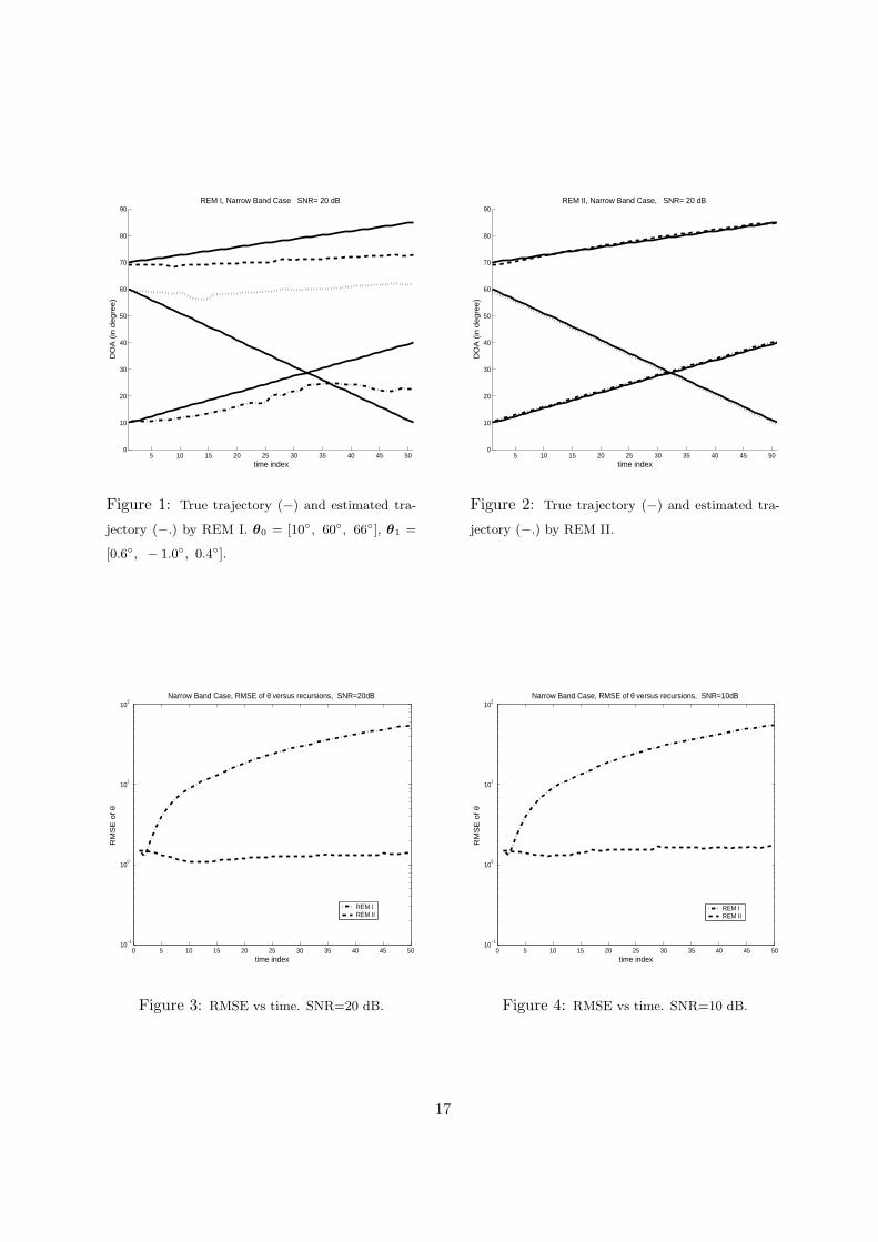
In the first experiment, we consider relatively fast moving sources. The true parameters are

given by θ0 = [10◦, 60◦, 66◦], θ1 = [0.6◦, − 1.0◦, 0.4◦] where θ1 is measured by degree per time

unit. In order to get a good insight into the tracking behavior, the same initial values are used

in all trials. We applied LPA based beamforming to 20 snapshots to obtain the initial estimates

θ00 = [10.5◦, 59.5◦, 68.5◦], θ0

1 = [0.58◦, − 0.99◦, 0.38◦]. The initial estimate for REM I is given

by θ00. Both algorithms use a constant step size ǫ = 0.6. Figs. 1 and 2 present the true values

of θ and an example of estimated trajectories. As shown in both figures, two source directions

cross with each other at t = 32. Obviously, the recursive procedure designed for the most general

case can not follow fast moving sources at all. In contrast, the estimated trajectory obtained by

REM II is very close to the true one. Figs. 3 and 4 show the mean square errors (RMSE) of

the DOA estimates, defined as√

‖θt − θ‖2 , averaged over 200 trials. Since REM I fails to track

the moving sources, the corresponding RMSE grows with increasing time. On the other hand,

the RMSE associated with REM II decreases slightly at the beginning of the recursion and then

remains almost constant. Comparing Figs. 3 and 4, one can observe that SNR= 20 dB has a

slightly lower RMSE than SNR= 10 dB.

The second experiment involves three slowly moving sources. The true parameter values are

given by θ0 = [30◦, 50◦, 62◦], θ1 = [0.06◦, − 0.1◦, 0.05◦]. Note that the angular velocity θ1 is

approximately 1/10 of that considered in the previous experiment. We applied the ML method

to obtain the initial estimates θ00 = [30.1◦, 50.8◦, 60.9◦]. Because the angular velocity is very

small compared to that in the previous experiment, we take θ01 = [0◦, 0◦, 0◦] as the initial value

for θ1. The initial estimate for REM I is given by θ00. Both algorithms use a constant step

size ǫ = 0.6. Figs. 5 and 6 present the true and estimated trajectories obtained by REM I and

REM II. Similarly to the first experiment, two source directions cross with each other at t = 126.

The estimated trajectory by REM I is close to the true one when no crossing happens. Between

t = 100 and t = 230 where two source directions cross with each other, the estimated trajectories

associated with the first two sources do not get close to each other. Instead, they just depart in

the vicinity of t = 126. For the same scenario, REM II provides a more accurate estimate. Fig. 6

shows that the crossing point causes a larger deviation from the true trajectory. Due to a higher

sensitivity to the variation of angular velocity at the crossing point, the estimated trajectory in

11

fig. 6 is slightly worse than that in fig. 2. Comparison of figs. 7 and 8 with figs. 3 and 4, shows

an overall lower RMSE in this scenario. Although REM I provides more reliable estimates than

in the first experiment, REM II still outperforms REM I.

In the third experiment, three sources move slowly with different speeds but do not cross with

each other. The true parameters are given by θ0 = [10◦, 30◦, 62◦], θ1 = [0.08◦, 0.1◦, 0.06◦].

The initial estimates are θ00 = [10.04◦, 30.04◦, 62.05◦], θ0

1 = [0◦, 0◦, 0◦]. We use a constant step

size ǫ = 0.6. Both algorithms have good tracking ability. Figs. 9 and 10, show that RMSE is the

lowest among all three scenarios. REM II has a better performance than REM I. While REM II

has a better performance at higher SNR, REM I seems to be less sensitive to SNRs in all three

scenarios.

In addition to the narrow band signals, we also applied REM I and II to broadband signals

with 3 frequency bins. The scenario similar to the second experiment leads to results presented

in figs. 11 to 12. The estimates behave similar to the narrow band case. Comparison of RMSEs

shows that more frequency bins leads to higher accuracy.

5.2 Comparison with LPA beamforming

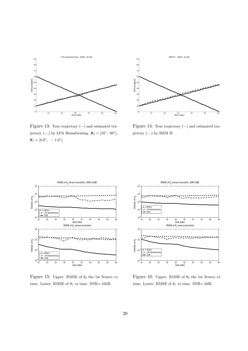
We compare REM II with the LPA based beamforming approach suggested by Katkovnik and

Gershman [17]. Both algorithms assume the motion model (17). In the first experiment, the

narrow band signals are generated by the following parameter set θ0 = [10◦, 60◦], θ1 = [0.6◦, −

1.0◦], SNR= 0, 10 dB. In the second experiment, we consider moving sources with lower angular

velocities θ0 = [30◦, 50◦], θ1 = [0.06◦, − 0.1◦]. A sliding window of 25 snapshots is used in the

LPA beamforming. The REM II is initialized by the LPA beamforming in the first scenario and

ML method in the second one. To ensure the same data length in each time interval, we use

additional (W − 1) samples in the LPA beamforming processing.

The estimated trajectories presented in figs. 13 and 14 are very close to the true ones. The

RMSEs of θ0 and θ1 corresponding to the first source are plotted in figs. 15 and 16. Using the

initial value provided by LPA beamforming, RMSE associated with REM II changes slowly over

the time. While estimates of θ0 remains constant, the estimates of θ1 become more accurate

with increasing recursions. Also, we can observe that while LPA beamforming provides an overall

better θ0 estimates, and a better angular velocity estimates at beginning of the recursion, REM

II improves θ1 estimates with increasing time and has less fluctuations.

12

Compared with the Cramer-Rao bounds (CRB) [21] plotted in solid lines (−), one realizes

that an REM II is certainly not efficient estimator. However, the ML approach suggested in [21],

whose estimation accuracy is close to CRB, is a batch processing and requires a complicated

multi-dimensional search procedure.

In the second experiment, REM II provides much more accurate estimates than LPA beam-

forming. Fig 17 shows that LPA beamforming even fails to follow the moving sources. We can

observed in fig 19 that REM II has lower RMSE in both θ0 and θ1 estimation. Consequently, as

shown in fig 20 the resulting DOA estimates are much better than LPA beamforming. In both

experiments, the computational time needed for LPA beamforming is about 800 times as high

as that required by REM II due to the two dimensional search procedure.

We conclude that REM I is suitable for tracking slowly time-varying DOA parameters, REM

II performs well for both slowly and fast moving sources. Both procedures generate accurate

estimates when there is no crossing point. When two source directions coincide with each other,

the steering matrix H(θ) becomes rank deficient. The signal waveform s(t) can not be deter-

mined properly. Consequently the DOA parameter can not be estimated accurately. In this

case, regularization is needed [21]. Since REM II incorporates a linear polynomial model, it has

a better tracking ability than REM I when this critical situation occurs. Compared to LPA

beamforming, our method has a clear computational advantage. It provides comparable results

with LPA beamforming in the fast moving sources case and outperforms LPA beamforming in

the slow moving source case. In addition, recursive EM is applicable to both narrow band and

broad band signals.

6 Conclusion

We addressed the problem of tracking multiple moving sources. Two recursive procedures are

proposed to estimate the time-varying DOA parameter. We applied the recursive EM algorithm

to a general case in which the motion of the sources is arbitrary and a specific case in which the

motion of sources is described by a linear polynomial model. Because of the simple structure

of the gain matrix, the suggested procedures are easy to implement. Furthermore, extension

of our approaches to broadband signals is straightforward. Numerical experiments showed that

our approaches provide excellent results in a slowly changing environment. When the DOA

parameter changes fast or two source directions cross with each other, the procedure derived

13

for a linear polynomial model has a better performance than the general procedure. Important

issues such as step size design and convergence analysis are still under investigation.

Acknowledgments

The authors thank the anonymous reviews for their constructive comments that significantly

improved the manuscript and also thank Associate Editor J. C. Chen for coordinating a speedy

review.

References

[1] A. Benveniste, M. Metivier and P. Priouret, Adaptive Algorithms and Stochastic Approxi-

mations, Springer Verlag, 1990.

[2] J. F. Bohme, “Array Processing”, Advances in Spectrum Analysis and Array Processing, pp.

1–63, Editor S. Haykin, Prentice Hall, Englewood Cliffs, N.J., 1991.

[3] J. F. Bohme, “ Statistical Array Signal Processing of Measured Sonar and Seismic Data”,

Proc. SPIE 2563 Advanced Signal Processing Algorithms, pp. 2–20, San Diego, July 1995.

[4] D. R. Brillinger, Time Series: Data Analysis and Theory, Holden-Day, 1981, San Francisco.

[5] Erdinc Cekli and Hakan A. Cyrpan, ”Unconditional Maximum Likelihood Approach for Lo-

calization of Near-Field Sources: Algorithm and Performance Analysis,” AEU International

Journal of Electronics and Communications, Vol. 57, No. 1, pp. 9-15, 2003

[6] P. J. Chung and J. F. Bohme, “Recursive EM and SAGE Algorithms”, Proc. IEEE Workshop

on Statistical Signal Processing, pp. 540–542, Singapore, August, 2001.

[7] P. J. Chung, “Fast Algorithms for Parameter Estimation of Sensor Array Signals”, Doctoral

thesis, Dept. of Electrical Engineering and Information Sciences, Ruhr-Universitat Bochum,

Universitatsverlag Bochum, May, 2002.

[8] P. J. Chung and J. F. Bohme, “DOA Estimation of Multiple Moving Sources Using Recur-

sive EM Algorithms”, Proc. Sensor Array and Multi-channel Signal Processing Workshop,

Washington DC, USA, August, 2002.

14

[9] P. J. Chung, Johann F. Bohme: “ Recursive EM and SAGE Algorithms with Application

to DOA Estimation”, submitted to IEEE Transactions on Signal Processing, 2003.

[10] P. J. Chung, J. F. Bohme: “Recursive EM Algorithm with Adaptive Step Size”, Proc. The

Seventh International Symposium on Signal Processing and Its Applications, Paris, France,

July 1–4, 2003.

[11] A. P. Dempster and N. Laird and D. B. Rubin, ”Maximum Likelihood from Incomplete

Data via the EM Algorithm”, Journal of the Royal Statistical Society, B39:1–38, 1977.

[12] M. Feder and E. Weinstein, “Parameter estimation of Superimposed Signals Using the EM

Algorithm” IEEE Trans. on ASSP , 36(4):477-489, April 1988.

[13] L. Frenkel and M. Feder, “Recursive Expectation and Maximization (EM) Algorithms for

Time–varying Parameters with Application to Multiple Target Tracking”, IEEE Trans.

Signal Processing, 47(2):306–320, February 1999.

[14] G. H. Golub and C. F. Van Loan, Matrix Computations, 3rd Edition, John Hopkins Uni-

versity Press, 1996.

[15] D. Maiwald, “Breitbandverfahren zur Signalentdeckung und –ortung mit Sensorgruppen

in Seismik– und Sonaranwendungen”, Doctoral thesis, Dept. of Electrical Engineering and

Information Sciences, Ruhr-Universitat Bochum , Shaker Verlag, Aachen, 1995.

[16] Nihat Kabaoglu, Hakan A. Cirpan, Erdinc Cekli and Selcuk Paker, ”Deterministic Maximum

Likelihood Approach for 3-D Near-Field Source Localization”, AEU International Journal

of Electronics and Communications, Vol. 57, No. 5, pp. 345-350, 2003.

[17] V. Katkovnik and A. B. Gershman, “ A Local Polynomial Approximation Based Beam-

forming for Source Localization and Tracking in Nonstationary Environments” IEEE Signal

Processing Letters, 7(1):3-5, January 2000.

[18] D. M. Titterington, “ Recursive Parameter Estimation using Incomplete Data”, J. R. Statist.

Soc. B, 46(2):257–267, 1984.

[19] D. M. Titterington and A. F. Smith and U. E. Makov “Statistical Analysis of Finite Mixture

Distributions”, John Wiley & Sons, New York, 1985.

15

[20] M. Wax and I. Ziskind, “Detection of the Number of Coherent Signals by the MDL Princi-

ple”, IEEE Trans. Acoust., Speech., Signal Processing, 37(8):1190-1196, 1989.

[21] T. Wigern and Eriksson, “Accuracy Aspects of DOA and Angular Velocity Estimation in

Sensor Array Processing”, IEEE Signal Processing Letters, 2(4), April 1995

[22] B. Yang, “Projection Approximation Subspace Tracking”, IEEE Trans. Signal Processing,

43(1):95-107, January 1995.

[23] R. E. Zarnich and K. L. Bell and H. L. Van Trees, “A unified Method for Mesurements

and Tracking of Contacts From an Array of Sensors”, IEEE Trans. Signal Processing,

49(12):2950-2961, December 2001.

16

5 10 15 20 25 30 35 40 45 500

10

20

30

40

50

60

70

80

90

time index

DO

A (

in d

eg

ree

)

REM I, Narrow Band Case SNR= 20 dB

Figure 1: True trajectory (−) and estimated tra-

jectory (−.) by REM I. θ0 = [10◦, 60◦, 66◦], θ1 =

[0.6◦, − 1.0◦, 0.4◦].

5 10 15 20 25 30 35 40 45 500

10

20

30

40

50

60

70

80

90

time indexD

OA

(in

de

gre

e)

REM II, Narrow Band Case, SNR= 20 dB


jectory (−.) by REM II.

0 5 10 15 20 25 30 35 40 45 5010

−1

100

101

102

time index

RM

SE

of θ

Narrow Band Case, RMSE of θ versus recursions, SNR=20dB

REM IREM II

Figure 3: RMSE vs time. SNR=20 dB.

0 5 10 15 20 25 30 35 40 45 5010

−1

100

101

102

time index

RM

SE

of θ


REM IREM II


17

50 100 150 200 250 3000

10

20

30

40

50

60

70

80

90

time index

DO

A (

in d

eg

ree

)

REM I, Narrow Band Case SNR= 20 dB


jectory (−.) by REM I. θ0 = [30◦, 50◦, 62◦], θ1 =

[0.06◦, − 0.1◦, 0.05◦].

50 100 150 200 250 3000

10

20

30

40

50

60

70

80

90

time indexD

OA

(in

de

gre

e)

REM II, Narrow Band Case, SNR= 20 dB



0 50 100 150 200 250 30010

−1

100

101

102

time index

RM

SE

of θ


REM IREM II


0 50 100 150 200 250 30010

−1

100

101

102

time index

RM

SE

of θ


REM IREM II


18

0 50 100 150 200 25010

−1

100

101

102

time index

RM

SE

of θ


REM IREM II

Figure 9: RMSE vs time. SNR=20 dB. θ0 =

[10◦, 30◦, 62◦], θ1 = [0.08◦, 0.1◦, 0.06◦].

0 50 100 150 200 25010

−1

100

101

102

time index

RM

SE

of θ


REM IREM II


0 50 100 150 200 250 30010

−1

100

101

102

time index

RM

SE

of θ

Broad Band Case, RMSE of θ versus recursions, SNR=20dB

REM IREM II

Figure 11: RMSE vs time. SNR=20 dB. θ0 =

[30◦, 50◦, 62◦], θ1 = [0.06◦, −0.1◦, 0.05◦]. Number

of frequency bins = 3.

0 50 100 150 200 250 30010

−1

100

101

102

time index

RM

SE

of θ

Broad Band Case, RMSE of θ versus recursions, SNR=10dB

REM IREM II


19

10 20 30 40 50 600

10

20

30

40

50

60

70

80

90

time index

DO

A (in

deg

ree)

LPA beamforming SNR= 10 dB


jectory (−.) by LPA Bemaforming. θ0 = [10◦, 60◦],

θ1 = [0.6◦, − 1.0◦].

10 20 30 40 50 600

10

20

30

40

50

60

70

80

90

time index

DO

A (in

deg

ree)

REM II SNR= 10 dB



15 20 25 30 35 40 45 50 55 6010

−2

10−1

100

101

102

time index

RM

SE

of θ 0

RMSE of θ0 versus recursions SNR=10dB

REM IILPA BeamformingCRB

15 20 25 30 35 40 45 50 55 6010

−3

10−2

10−1

100

time index

RM

SE

of θ 1

RMSE of θ1 versus recursions


Figure 15: Upper: RMSE of θ0 the 1st Source vs

time. Lower: RMSE of θ1 vs time. SNR= 10dB.

15 20 25 30 35 40 45 50 55 6010

−2

10−1

100

101

102

time index

RM

SE

of θ 0



15 20 25 30 35 40 45 50 55 6010

−3

10−2

10−1

100

time index

RM

SE

of θ 1





20

10 20 30 40 50 600

10

20

30

40

50

60

70

80

90

time index

DO

A (in

deg

ree)

LPA beamforming SNR= 10 dB


jectory (−.) by LPA Bemaforming. θ0 = [30◦, 50◦],

θ1 = [0.06◦, − 0.1◦].

10 20 30 40 50 600

10

20

30

40

50

60

70

80

90

time index

DO

A (in

deg

ree)

REM II SNR= 10 dB



15 20 25 30 35 40 45 50 55 6010

−2

10−1

100

101

102

time index

RM

SE

of θ 0



15 20 25 30 35 40 45 50 55 6010

−3

10−2

10−1

100

time index

RM

SE

of θ 1





15 20 25 30 35 40 45 50 55 6010

−1

100

101

102

time index

RM

SE

of θ

RMSE of θ, SNR=10dB

REM IILPA Bemaforming

Figure 20: RMSE of θ vs time.

21

Tracking of Multiple Moving Sources Using Recursive EM...

Documents

Transcript of Tracking of Multiple Moving Sources Using Recursive EM...