1

Tracking Gaze and Visual Focus of Attention ofPeople Involved in Social Interaction

Benoit Massé, Silèye Ba, and Radu Horaud

Abstract—The visual focus of attention (VFOA) has beenrecognized as a prominent conversational cue. We are interestedin estimating and tracking the VFOAs associated with multi-party social interactions. We note that in this type of situationsthe participants either look at each other or at an object ofinterest; therefore their eyes are not always visible. Consequentlyboth gaze and VFOA estimation cannot be based on eye detectionand tracking. We propose a method that exploits the correlationbetween eye gaze and head movements. Both VFOA and gazeare modeled as latent variables in a Bayesian switching state-space model. The proposed formulation leads to a tractablelearning procedure and to an efficient algorithm that simulta-neously tracks gaze and visual focus. The method is tested andbenchmarked using two publicly available datasets that containtypical multi-party human-robot and human-human interactions.

Index Terms—Visual focus of attention, eye gaze, head pose,dynamic Bayesian model, switching Kalman filter, multi-partydialog, human-robot interaction.

I. INTRODUCTION

In this paper we are interested in the computational analysisof social interactions. In addition to speech, people com-

municate via a large variety of non-verbal cues, e.g. prosody,hand gestures, body movements, head nodding, eye gaze, andfacial expressions. For example, in a multi-party conversation,a common behavior consists in looking either at a person,e.g. the speaker, or at an object of current interest, e.g. acomputer screen, a painting on a wall, or an object lying ona table. We are particularly interested in estimating the visualfocus of attention (VFOA), or who is looking at whom or atwhat, which has been recognized as one of the most prominentsocial cues. It is used in multi-party dialog to establish face-to-face communication, to respect social etiquette, to attractsomeone’s attention, or to signify speech-turn taking, thuscomplementing speech communication.

The VFOA characterizes a perceiver/target pair. It may bedefined either by the line from the perceiver’s face to theperceived target, or by the perceiver’s direction of sight or gazedirection (which is often referred to as eye gaze or simplygaze). Indeed, one may state that the VFOA of person i istarget j if the perceiver’s gaze is aligned with the perceiver-to-target line. From a physiological point of view, eye gazedepends on both eyeball orientation and head orientation. Boththe eye and the head are rigid bodies with three and six degreesof freedom respectively. The head position (three coordinates)and the head orientation (three angles) are jointly referred to

B. Massé and R. Horaud are with INRIA Grenoble Rhône-Alpes, Mont-bonnot Saint-Martin, France.

S. Ba is with Dailymotion, Paris, FranceThis work is supported by ERC Advanced Grant VHIA #340113.

as the head pose. With proper choices for the head- and eye-centered coordinate frames, one can assume that gaze is acombination of head pose and of eyeball orientation,1 and theVFOA depends on head pose, eyeball orientation, and targetlocation.

In this paper we are interested into estimating and trackingjointly the VFOAs of a group of people that communicate witheach other and with a robot, or multi-party HRI (human-robotinteraction), which may well be viewed as a generalizationof single-user HRI. From a methodological point of view theformer is more complex than the latter. Indeed, in single-userHRI the person and the robot face each other and hence acamera mounted onto the robot head provides high-resolutionfrontal images of the user’s face such that head pose andeye orientation can both be easily and robustly estimated.In the case of multi-party HRI the eyes are barely detectedsince the participants often turn their faces away from thecamera. Consequently, VFOA estimation methods based oneye detection and eye tracking are ineffective and one has toestimate the VFOA, indirectly, without explicit eye detection.

We propose a Bayesian switching dynamic model for theestimation and tracking gaze directions and VFOAs of severalpersons involved in social interaction. While it is assumedthat head poses (location and orientation) and target locationscan be directly detected from the data, the unknown gazedirections and VFOAs are treated as latent random variables.The proposed temporal graphical model, that incorporates gazedynamics and VFOA transitions, yields (i) a tractable learn-ing algorithm and (ii) an efficient gaze-and-VFOA trackingmethod.2 The proposed method may well be viewed as acomputational model of [1], [2].

The method is evaluated using two publicly availabledatasets, Vernissage [3] and LAEO [4]. These datasets consistof several hours of video containing situated dialog betweentwo persons and a robot (Vernissage) and human-humaninteractions (LAEO). We are particularly interested in findingparticipants that either gaze to each other, gaze to the robot,or gaze to an object. Vernissage is recorded with a motioncapture system (a network of infrared cameras) and with acamera placed onto the robot head. LAEO is collected fromTV shows.

1Note that orientation generally refers to the pan, tilt and roll angles ofa rigid-body pose, while direction refers to the polar and azimuth angles or,equivalently, a unit vector. Since the contribution of the roll angle to gaze isgenerally marginal, in this paper we make no distinction between orientationand direction.

2Supplementary materials, that include a software package and examplesof results, are available at https://team.inria.fr/perception/research/eye-gaze/.

arX

iv:1

703.

0472

7v2

[cs

.CV

] 2

1 N

ov 2

017

2

The remainder of this paper is organized as follows. Sec-tion II provides an overview of related work in gaze, VFOAand head-pose estimation. Section III introduces the paper’smathematical notations and definitions, states the problemformulation and describes the proposed model. Section IVpresents in detail the model inference and Section V derivesthe learning algorithm. Section VI provides implementationdetails and Section VII describes the experiments and reportsthe results.

II. RELATED WORK

As already mentioned, the VFOA is correlated with gaze.Several methods proceed in two steps, in which the gazedirection is estimated first, and then used to estimate VFOA.In scenarios that rely on precise estimation of gaze [5], [6]a head-mounted camera, like the one in [7], can be usedto detect the iris with high accuracy. Head-mounted eyetrackers provide extremely accurate gaze measurements and insome circumstances eye-tracking data can be used to estimateobjects of interest in videos [8]. Nevertheless, they are invasiveinstruments and hence not appropriate for analyzing socialinteractions.

Gaze estimation is relevant for a number of scenarios, suchas car driving [9] or interaction with smartphones [10]. In thesesituations, either the field of view is limited, hence the range ofgaze directions is constrained (car driving), or active humanparticipation ensures that the device yields frontal views ofthe user’s face, thus providing accurate eye measurements [7],[9], [11], [12]. In some scenarios the user is even asked tolimit head movements [13], or to proceed through a calibrationphase [12], [14]. Even if no specific constraints are imposed,single-user scenarios inherently facilitate the task of eye mea-surement [11]. At the best of our knowledge, there is no gazeestimation method that can deal with unconstrained scenarios,e.g. participants not facing the cameras, partially or totallyoccluded eyes, etc. In general, eye analysis is inaccurate whenparticipants are faraway from the camera.

An alternative is to approximate gaze direction with headpose [15]. Unlike eye-based methods, head pose can beestimated from low-resolution images, i.e. distant cameras[16], [17], [18], [19], [20]. These methods estimate gazeonly approximatively since eyeball orientation can differ fromhead orientation by ±35° [21]. Gaze estimation from headorientation can benefit from the observation that gaze shiftsare often achieved by synchronously moving the head and theeyes [22], [1], [2]. The correlation between head pose and gazehas also been exploited in [23]. More recently, [24] combinedhead and eye features to estimate the gaze direction using anRGB-D camera. The method still requires that both eyes arevisible.

Several methods were proposed to infer VFOAs either fromgaze directions [25], or from head poses [4], [26], [27], [28].For example, in [4] it is proposed to build a gaze cone aroundthe head orientation and targets lying inside this cone are usedto estimate the VFOA. While this method was successfullyapplied to movies, its limitation resides in its vagueness: theVFOA information is limited to whether there are two peoplelooking at each other or not.

An interesting application of VFOA estimation it the anal-ysis of social behavior of participants engaged in meetings,e.g. [23], [26], [29], [30]. Meetings are characterized byinteractions between seated people that interact based onspeech and on head movements. Some methods estimate themost likely VFOA associated with a head orientation [23],[29]. The drawback of these approaches is that they must bepurposively trained for each particular meeting layout. Thecorrelation between VFOA and head pose was also investi-gated in [26] where an HMM is proposed to infer VFOAsfrom head and body orientations. This work was extendedto deal with more complex scenarios, such as participantsinteracting with a robot [27], [31]. An input-output HMM isproposed in [31] to enable to model the following contextualinformation: participants tend to look to the speaker, to therobot, or to an object which is referred to by the speaker orby the robot. The results of [31] show that this improves theperformance of VFOA estimation. Nevertheless, this methodrequires additional information, such as speaker identificationor speech recognition.

The problem of joint estimation of gaze and of VFOAwas addressed in a human-robot cooperation task [28]. Insuch a scenario the user doesn’t necessarily face the cameraand robot-mounted cameras have low-resolution, hence theestimation of gaze from direct analysis of eye regions is notfeasible. [28] proposes to learn a regression between the spaceof head poses and the space of gaze directions and thento predict an unknown gaze from an observed head pose.The head pose itself is estimated by fitting a 3D ellipticalcylinder to a detected face, while the associated gaze directioncorresponds to the 3D line joining the head center to thetarget center. This implies that during the learning stage,the user is instructed to gaze at targets lying on a tablein order to provide training data. The regression parametersthus estimated correspond to a discrete set of head-pose/gaze-direction pairs (one for each target); an erroneous gaze may bepredicted when the latter is not in the range of gaze directionsused for training.

A summary of the proposed Bayesian dynamic model andexperiments with the Vernissage [3] motion capture datasetwere presented in [32]. In this article we provide a detailedand comprehensive description and analysis of the proposedmodel, of the model inference, of the learning methodology,and of the associated algorithms. We show results with bothmotion capture and RGB data from Vernissage. Additionally,we show results with the LAEO dataset [4].

III. PROPOSED MODEL

The proposed mathematical model model is inspired frompsychophysics [1], [2]. In unconstrained scenarios a personswitches his/her gaze from one target to another target,possibly using both head and eye movements. Quick eyemovements towards a desired object of interest are calledsaccades. Eye movements can also be caused by the vestibule-ocular reflex that compensates for head movements such thatone can maintain his/her gaze in the direction of the target ofinterest. Therefore, in the general case, gazing to an object isachieved by a combination of eye and head movements.

3

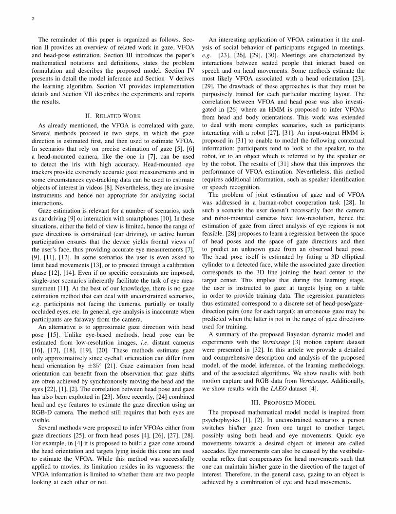
Figure 1. This figure illustrates the principle of our method and displays the observed and latent variables associated with a person (left-person indexed byi). The two images were grabbed with a camera mounted onto the head of a robot and they correspond to frames t − n (left image) and t (right image),respectively. The following variables are displayed: head orientation (red arrow), Hi

t−n,Hit (observed variables), as well as the latent variables estimated

with the proposed method, namely gaze direction (green arrow), Git−n,G

it, VFOA, Vi

t−n,Vit, and head reference orientation (black arrow), Ri

t−n,Rit

(that coincides with upper-body orientation). In this example left-person gazes towards the robot at t − n, then turns her head to eventually gaze towardsright-person at t, hence her VFOA switches from Vi

t−n = robot to Vit = right-person.

In the case of small gaze shifts, e.g. reading or watchingTV, eye movements are predominant. In the case of largegaze shifts, often needed in social scenarios, head movementsare necessary since eyeball movements have limited range,namely ±35° [21]. Therefore, the proposed model considersthat gaze shifts are produced by head movements that occursimultaneously with eye movements.

A. Problem Formulation

We consider a scenario composed of N active targets andM passive targets. An active target is likely to move and/or tohave a leading role in an interaction. Active targets are personsand robots.3 Passive targets are objects, e.g. wall paintings.The set of all targets is indexed from 0 to N + M , wherethe index 0 designates “no target". Let i be an active target (aperson or a robot), 1 ≤ i ≤ N , and j be a passive target (anobject), N + 1 ≤ j ≤ N +M . A VFOA is a discrete randomvariable defined as follows: Vi

t = j means person (or robot) ilooks at target j at time t. The VFOA of a person (or robot)i that looks at none of the known targets is Vi

t = 0. The caseVit = i is excluded. The set of all VFOAs at time t is denoted

by Vt =(V1t , . . . ,V

Nt

).

Two continuous variables are now defined: head orientationand gaze direction. The head orientation of person i at tis denoted with Hi

t = [φiH,t, θiH,t]>, i.e. the pan and tilt

angles of the head with respect to some fixed coordinateframe. The gaze direction of person i is denoted with Gi

t

and is also parameterized by pan and tilt with respect to thesame coordinate frame, namely Gi

t = [φiG,t, θiG,t]>. Although

eyeball orientation is neither needed nor used, it is worthnoticing that it is the difference between Gi

t and Hit. These

variables are illustrated on Fig. 1.

3Note that in case of a robot, the gaze direction and the head orientationare identical and that the latter can be easily estimated from the head motors.

Finally, to establish a link between VFOAs and gaze di-rections, the target locations must be defined as well. LetXit = [xit, y

it, z

it]> be the location of target i. In the case

of a person, this location corresponds to the head centerwhile in the case of a passive target, it corresponds to thetarget center. These locations are defined in the same coor-dinate frame as above. Also notice that the direction fromthe active target i to target j is defined by the unit vectorXijt = (Xj

t−Xit)/‖X

jt−Xi

t‖ which can also be parameterizedby two angles, Xij

t = [φi,jX,t, θi,jX,t]>.

As already mentioned, target locations and head orientationsare observed random variables, while VFOAs and gaze direc-tions are latent random variables. The problem to be solvedcan now be formulated as a maximum a posteriori (MAP)problem:

Vt, Gt = argmaxVt,Gt

P (Vt,Gt|H1:t,X1:t) (1)

Since there is no deterministic relationship between headorientation and gaze direction, we propose to model it prob-abilistically. For this purpose, we introduce an additionallatent random variable, namely the head reference orientation,Rit = [φiR,t, θ

iR,t]>, which we choose to coincide with

the upper-body orientation. We use the following generativemodel, initially introduced in [26], linking gaze direction, headorientation, and head reference orientation:

P (Hit|Gi

t,Rit;α,ΣH) = N (Hi

t;µiH,t,ΣH), (2)

with µiH,t = αGit + (I2 −α)Ri

t, (3)

where ΣH ∈ R2×2 is a covariance matrix, I2 ∈ R2×2 is theidentity matrix and α = Diag (α1, α2) is a diagonal matrixof mixing coefficients, 0 < α1, α2 < 1. Also it is assumedthat the covariance matrix is the same for all the persons andover time. Therefore, head orientation is an observed randomvariable normally distributed around a convex combination

4

Gt−1 Gt

Ht−1 Ht

Rt−1 Rt

Xt−1 Xt

Vt−1 Vt

Figure 2. Graphical representation showing the dependencies between thevariables of the proposed Bayesian dynamic model. The discrete latentvariables (visual focus of attention) are shown with squares while continuousvariables are shown with circles: observed variables (head pose and targetlocations) are shown with shaded circles and latent variables (gaze andreference) are shown with white circles.

between two latent variables: gaze direction and head referenceorientation.

B. Gaze Dynamics

The following model is proposed:

P (Git|Gi

t−1Git−1,V

it = j,Xt) = N (Gi

t;µijG,t,ΓG), (4)

P (Git|Gi

t−1) = N (Git; G

it−1,ΓG), (5)

with:

µijG,t =

{Git−1 + Gi

t−1 dt, if j = 0,

βGit−1 + (I2 − β)Xij

t + Git−1 dt, if j 6= 0,

(6)

where Git = dGi

t/dt is the gaze velocity, ΓG,ΓG ∈ R2×2

are covariance matrices, and β = Diag (β1, β2) is a diagonalmatrix of mixing coefficients, 0 < β1, β2 < 1. Therefore, if aperson looks at one of the targets, then his/her gaze dynamicsdepends on the person-to-target direction Xij

t at a rate equalto β, and if a person doesn’t look at one of the targets, thenhis/her gaze dynamics follows a random walk.

The head reference orientation dynamics can be defined ina similar way:

P (Rit|Ri

t−1, Rit−1) = N (Ri

t;µiR,t,ΓR), (7)

P (Rit|Ri

t−1) = N (Rit; R

it−1,ΓR), (8)

with µiR,t = Rit−1 + Ri

t−1 dt,

where Rit = dRi

t/dt is the head reference orientation velocityand ΓR,ΓR ∈ R2×2 are covariance matrices. The dependen-cies between all the model variables are shown as a graphicalrepresentation in Figure 2.

It is assumed that the gaze directions associated with differ-ent people are independent, given the VFOAs V1:t. The cross-dependency between different people is taken into accountby the VFOA dynamics as detailed in section III-C below.Similarly, head orientations, and head reference orientations

associated with different people are independent, given theVFOAs. By combining the above equations with this inde-pendency assumption, we obtain:

P (Ht|Gt,Rt) =∏i

N (Hit;µ

iH,t,ΣH) (9)

P (Gt|Gt−1, Gt−1,Vt,Xt) =∏i,j

N (Git;µ

ijG,t,ΓG)δj(V

it)

(10)

P (Rt|Rt−1, Rt−1) =∏i

N (Rit;µ

iR,t,ΓR) (11)

where the dependencies between variables are embedded inthe variable means, i.e. (3) and (6). The covariance matriceswill be estimated via training. While gaze directions can varya lot, we assume that head reference orientations are almostconstant over time, which can be enforced by imposing thatthe total variance of gaze is much larger than the total varianceof head reference orientation, namely:

Tr(ΓG)� Tr(ΓR), (12)

C. VFOA Dynamics

Using a first-order Markov approximation, the VFOA tran-sition probabilities can be written as:

P (Vt|V1:t−1) = P (Vt|Vt−1), (13)

Notice that matrix P (Vt|Vt−1) is of size (N +M)N × (N +M)N . Indeed, there are N persons (active targets), and N +M+1 targets (one "no" target, N active targets and M passivetargets) and the case of a person that looks to him/herself isexcluded. For example, if N = 2 and M = 4, matrix (13)has (2 + 4)2×2 = 1296 entries. The estimation of this matrixwould require, in principle, a large amount of training data, inparticular in the presence of many symmetries. We show that,in practice, only 15 different transitions are possible. This canbe seen on the following grounds.

We start by assuming conditional independence between theVFOAs at t:

P (Vt|Vt−1) =∏i

P (Vit|Vt−1). (14)

Let’s consider V it , the VFOA of person i at t, given Vt−1,the VFOAs at t− 1. One can distinguish two cases:• V it−1 = k where k is either a passive target, N < k ≤N + M , or it is none of the targets, k = 0; in this caseV it depends only on V it−1, and

• V it−1 = k, where k 6= i is a person 1 ≤ k ≤ N ; in thiscase V it depends on the both V it−1 and V kt−1.

To summarize, we can write that:

P (Vit = j|Vt−1) ={P (Vi

t = j|Vit−1 = k,Vk

t−1 = l) if 1 ≤ k ≤ N,P (Vi

t = j|Vit−1 = k) otherwise.

(15)

Based on this it is now possible to count the total numberof possible VFOA transitions. With the same notations as in(15), we have the following possibilities:

5

• k = 0 (no target): there are two possible transitions, j = 0and j 6= 0.

• N < k ≤ N+M (passive target): there are three possibletransitions, j = 0, j = k, and j 6= k.

• 1 ≤ k ≤ N, l = 0 (active target k looks at no target):there are three possible transitions, j = 0, j = k, andj 6= k.

• 1 ≤ k ≤ N, l = i (active target k looks at person i): thereare three possible transitions, j = 0, j = k, and j 6= k.

• 1 ≤ k ≤ N, l 6= 0, i (active target k looks at active target ldifferent than i): there are four possible transitions, j = 0,j = k, j = l and j 6= k, l.

Therefore, there are 15 different possibilities for P (Vit =

j|Vt−1), i.e. appendix A. Moreover, by assuming that theVFOA transitions don’t depend on i, we conclude that thetransition matrix may have up to 15 different entries. More-over, the number of possible transitions is even smaller if thereis no passive target (M = 0), or if the number of active targetsis small, e.g. N < 3. This considerably simplifies the task ofestimating this matrix and makes the task of learning tractable.

IV. INFERENCE

We start by simplifying the notation, namely Lt =[Gt; Gt; Rt; Rt] where [·; ·] denotes vertical concatenation.The emission probabilities (9) become:

P (Ht|Lt) =∏i

N (Hit;µ

iH,t,ΣH), (16)

with µiH,t = CLit, (17)

where matrix C is obtained from the definition of Lt aboveand from (3):

C =

(α1 0 0 0 1− α1 0 0 00 α2 0 0 0 1− α2 0 0

).

The transition probabilities can be obtained by combin-ing (10) and (11) with (5) and (8):

P (Lt|Vt,Lt−1,Xt) =∏i

∏j

N (Lit;µijL,t,ΓL)δj(V

it), (18)

with µijL,t = Aijt Lit−1 + bijt (19)

and ΓL =

ΓG

ΓG

ΓR

ΓR

, (20)

where Aijt is an 8 × 8 matrix and bijt is an 8 × 1 vector.

The indices i,j and t cannot be dropped since the transitionsdepend on Xij

t from (6).The MAP problem (1) can now be derived in a Bayesian

framework for the VFOA variables:

P (Vt|H1:t,X1:t) =

∫P (Vt,Lt|H1:t,X1:t)dLt. (21)

We propose to study the filtering distribution of the joint latentvariables, namely P (Vt,Lt|H1:t,X1:t). Indeed, Bayes ruleyields:

P (Vt,Lt|H1:t,X1:t) =1

cP (Ht|Lt)P (Lt,Vt|H1:t−1,X1:t).

(22)

where c is the normalization evidence. Now we can introduceVt−1 and Lt−1 using the sum rule:

P (Lt,Vt|H1:t−1,X1:t)

=∑Vt−1

∫P (Lt,Vt,Lt−1,Vt−1|H1:t−1,X1:t)dLt−1

=∑Vt−1

∫P (Lt|Vt,Lt−1,Xt)P (Vt|Vt−1)

× P (Lt−1,Vt−1|H1:t−1,X1:t−1)dLt−1, (23)

where unnecessary dependencies were removed. Combin-ing (22) and (23) we obtain a recursive formulation inP (Vt,Lt|H1:t,X1:t). However, this model is still intractablewithout further assumptions. The main approximation usedin this work consists of assuming local independence for theposteriors:

P (Lt,Vt|H1:t,X1:t) '∏i

P (Lit,Vit|H1:t,X1:t). (24)

A. Switching Kalman Filter Approximation

Several strategies are possible, depending upon the struc-ture of P (Lt,Vt|H1:t,X1:t). Commonly used strategies toevaluate this distribution include variational Bayes or Monte-Carlo. Alternatively, we propose to cast the problem into theframework of switching Kalman filters (SKF) [33]. We assumethe filtering distribution to be Gaussian,

P (Lt,Vt|H1:t,X1:t) ∝ N (Lt;µt,Σt). (25)

From (24) and (25) we obtain the following factorization:

P (Lt,Vt|H1:t,X1:t) ∝∏i

∏j

N (Lit;µijt ,Σ

ijt )δj(V

it). (26)

Thus, (23) can be split into N components, one for each activetarget i:

P (Lit,Vit = j|H1:t,X1:t) ∝ P (Hi

t|Lit)

×∑Vt−1

∫N (Lit;A

ijt Lit−1 + bijt )P (Vi

t|Vt−1)

×∏k

N (Lit−1;µikt−1,Σikt−1)δk(V

it−1)dLit−1, (27)

or, after several algebraic manipulations:

P (Lit,Vit = j|H1:t,X1:t) ∝

∑k

wijkt−1,tN (Lit;µijkt ,Σijk

t ).

(28)

In this expression, µijkt and Σijkt are obtained by performing

constrained Kalman filtering on µikt−1, Σikt−1 with transition

dynamics defined by Aijt and bijt , emission dynamics defined

by C, and observation Hit, i.e. [34]. The weights wijkt−1,t are

defined as P (Vit−1 = k | Vi

t = j,H1:t,X1:t). The constraintcomes from the fact that ||Gi

t −Hit|| < 35° and is achieved

by projecting the mean (refer to [34] for more details).This can be rephrased as follows: from the filtering dis-

tribution at time t − 1, there are N + M possible dynamicsfor Lit. The normal distribution at time t − 1 then becomes

6

a mixture of N + M normal distributions at time t asshown in (28). However, we expect a single Gaussian suchas P (Lit,V

it = j|H1:t,X1:t) ∝ N (Lit;µ

ijt ,Σ

ijt ). This can be

done by moment matching:

µijt =∑k

wijkt−1,tµijkt (29)

Σijt =

∑k

wijkt−1,t(Σijkt + (µijkt − µijt )(µijkt − µijt )>) (30)

Finally, it is necessary to evaluate wijkt−1,t. Let’s introducethe following notations:

cijkt−1,t = P (Vit = j,Vi

t−1 = k|H1:t,X1:t), (31)

cijt = P (Vit = j|H1:t,X1:t). (32)

It follows that

cijt =∑k

cijkt−1,t and wijkt−1,t =cijkt−1,t

cijt.

By applying Bayes formula to cijkt−1,t, yields:

cijkt−1,t ∝ P (Ht|Vit = j,Vi

t−1 = k,H1:t−1,X1:t)

×cikt−1P (Vit = j|Vi

t−1 = k,H1:t−1,X1:t−1) (33)

Then, cikt−1 is obtained from cijkt−2,t−1 calculated at pre-vious time step. The last factor in (33) is either equalto∑l cklt−1P (Vi

t = j|Vit−1 = k,Vk

t−1 = l) if k isan active target, or P (Vi

t = j|Vit−1 = k) otherwise.

Both cases are straightforward to compute. Finally, thefirst factor in (33), the observation component, can befactorized as P (Hi

t|Vit = j,Vi

t−1 = k,H1:t−1,X1:t) ×∏n 6=i

∑m

∑p P (Hn

t |Vnt = m,Vn

t−1 = p,H1:t−1,X1:t). Byintroducing the latent variable L, we obtain:

P (Hnt |Vn

t = m,Vnt−1 = p,H1:t−1,X1:t)

=

∫P (Hn

t |Lnt ) P (Lnt |Lnt−1,Vnt = m,Xt)

× P (Lnt−1|Vnt−1 = p,H1:t−1,X1:t−1)dLnt−1dL

nt . (34)

All the factors (34) are normal distributions, hence it inte-grates in closed-form. In summary, we devised a procedureto estimate an online approximation of the joint filteringdistribution of the VFOAs, Vt, and of the gaze and headreference directions, Lt.

V. LEARNING

The proposed model has two sets of parameters that mustbe estimated: the transition probabilities associated with thediscrete VFOA variables, and the parameters associated withthe Gaussian distributions. Learning is carried out using Qrecordings with annotated VFOAs. Each recording is com-posed of Tq frames, 1 ≤ q ≤ Q and contains Nq activetargets (the robot is the active target 1 and the persons areindexed from 2 to Nq) and Mq passive targets. In addition totarget locations and head poses, it is worth noticing that thelearning algorithm requires VFOA ground-truth annotations,while gaze directions are still treated as latent variables.

A. Learning the VFOA Transition Probabilities

The VFOA transitions are drawn from the generalizedBernoulli distribution. Therefore, the transition probabilitiescan be estimated with P (Vi

t = j|Vt−1) = Et−1[δj(Vit)],

where δj(i) is the Kronecker delta function. In Section III-Cwe showed that there are up to 15 different possibilities forthe VFOA transition probability. This enables us to derive anexplicit formula for each case, see appendix B. Consider forexample one of these cases, namely p14 = P (Vi

t = l|Vit−1 =

k,Vkt−1 = l), which is the conditional probability that at t

person i looks at target l, given that at t−1 person i looked atperson k and that person k looked at target l. This probabilitycan be estimated with the following formula:

p14 =

Q∑q=1

Nq∑i=2

Tq∑t=2

Nq∑k=1k 6=i

∑l 6=i,k

δl(Vq,it )δk(Vq,i

t−1)δl(Vq,kt−1)

Q∑q=1

Nq∑i=2

Tq∑t=2

Nq∑k=1k 6=i

∑l 6=i,k

δk(Vq,it−1)δl(V

q,kt−1)

B. Learning the Gaussian Parameters

In Section IV we described the derivation of the proposedmodel that is based on SKF. This model requires the param-eters (means and covariances) of the Gaussian distributionsdefined in (16) and (18). Notice however that the mean (17) of(16) is parameterized by α. Similarly, the mean (19) of (18) isparameterized by β. Consequently, the model parameters are:

θ = (α,β,ΓL,ΣH), (35)

and we remind that α and β are 2× 2 diagonal matrices, ΓL

is a 8× 8 covariance and and ΣH is a 2× 2 covariance, andthat we assumed that these matrices are common to all theactive targets. Hence the total number of parameters is equalto 2 + 2 + 36 + 3 = 43.

In the general case of SKF models, the discrete variablesare unobserved both for learning and for inference. Herewe propose a learning algorithm that takes advantage of thefact that the discrete variables, i.e. VFOAs, are observedduring the learning process, namely the VFOAs are annotated.We propose an EM algorithm adapted from [35]. In thecase of a standard Kalman filter, an EM iteration alternatesbetween a forward-backward pass to compute the expectedlatent variables (E-step), and between the maximization of theexpected complete-data log-likelihood (M-step).

We start by describing the M-step. The complete-data log-likelihood is:

lnP (L1,H1, . . . ,LQ,HQ|θ)

=

Q∑q=1

Nq∑i=2

Tq∑t=2

lnP (Lq,it |Lq,it−1,β,ΓL)

+

Q∑q=1

Nq∑i=2

Tq∑t=1

lnP (Hq,it |L

q,it ,α,ΣH). (36)

7

By taking the expectation w.r.t. the posterior distributionP (L1, . . . ,LQ|H1, . . . ,HQ,θ), we obtain:

Q(θ,θold) = EL1,...,LK |θold

[lnP (L1,H1, . . . ,LQ,HQ|θ)

],

(37)

which can be maximized w.r.t. to the parameters θ, whichyields closed-form expressions for the covariance matrices:

ΓL =

Q∑q=1

Nq∑i=2

Tq∑t=2

E[(Lq,it − µq,ijL,t )(Lit − µq,ijL,t )>]

Q∑q=1

(Nq − 1)(Tq − 1)

(38)

where µq,ijL,t = Aq,ijt Lq,it−1 + bq,ijt , i.e. (19), and:

ΣH =

Q∑q=1

Nq∑i=2

Tq∑t=1

E[(Hq,it − µq,iH,t)(H

q,it − µq,iH,t)

>]

Q∑q=1

(Nq − 1)Tq

, (39)

where µq,iH,t = CLq,it , i.e. (17).The estimation of α and of β is carried out in the following

way. ∂Q(θ,θold)/∂β1 = 0 and ∂Q(θ,θold)/∂β2 = 0 yield aset of two linear equations in the two unknowns:

Q∑q=1

Nq∑i=2

Tq∑t=2

E[(Lq,it − µq,ijL,t )>Γ−1L

∂

∂β1(Lq,it − µq,ijL,t )

]= 0,

Q∑q=1

Nq∑i=2

Tq∑t=2

E[(Lq,it − µq,ijL,t )>Γ−1L

∂

∂β2(Lq,it − µq,ijL,t )

]= 0,

(40)

and similarly:

Q∑q=1

Nq∑i=2

Tq∑t=1

E[(Hq,i

t − µq,iH,t)>Σ−1H

∂

∂α1(Hq,i

t − µq,iH,t)

]= 0,

Q∑q=1

Nq∑i=2

Tq∑t=1

E[(Hq,i

t − µq,iH,t)>Σ−1H

∂

∂α2(Hq,i

t − µq,iH,t)

]= 0,

(41)

where as above, the expectation is taken w.r.t. to the posteriordistribution. Once the formulas above are expanded and oncethe means µq,ijL,t and µq,iH,t are substituted with their expres-sions, the following terms remain to be estimated: E[Lq,it ],E[Lq,it Lq,it

>] and E[Lq,it Lq,it−1

>].

The E-step provides estimates of these expectations viaa forward-backward algorithm. For the sake of clarity, wedrop the superscripts i (active target index) and q (recordingindex) up to equation (48) below. Introducing the notationP (Lt|H1, . . . ,Ht) = N (Lt;µt,Pt), the forward-pass equa-tions are:

µt = Atµt−1 + bt + Kt(Ht −C(Atµt−1 + bt)) (42)Pt = (I−KtC)Pt,t−1, (43)

where:

Pt,t−1 = AtPt−1A>t + ΓL, (44)

Kt = Pt,t−1C>(CPt,t−1C

> + ΣH)−1. (45)

The backward pass estimates P (Lt|H1, . . . ,HT ) =N (Lt; µt, Pt) and leads to

µt = µt + Jt(µt+1 − (At+1µt + bt+1)), (46)

Pt = Pt + Jt(Pt+1 −Pt+1,t)J>t , (47)

where:

Jt = PtA>t+1(Pt+1,t)

−1. (48)

The expectations are estimated by performing a forward-backward pass over all the persons and all the recordings ofthe training data. This yields the following formulas:

E[Lq,it ] = µq,it (49)

E[Lq,it Lq,it>

] = Pq,it + µq,it µq,it

>(50)

E[Lq,it Lq,it−1>

] = Pq,it Jq,it−1

>+ µq,it µq,it−1

>(51)

VI. IMPLEMENTATION DETAILS

The proposed method was evaluated on the Vernissagedataset [3] and on the Looking At Each Other (LAEO)dataset [4]. We describe in detail these datasets and their an-notations. We provide implementation details and we analysethe complexity of the proposed algorithm.

A. The Vernissage Dataset

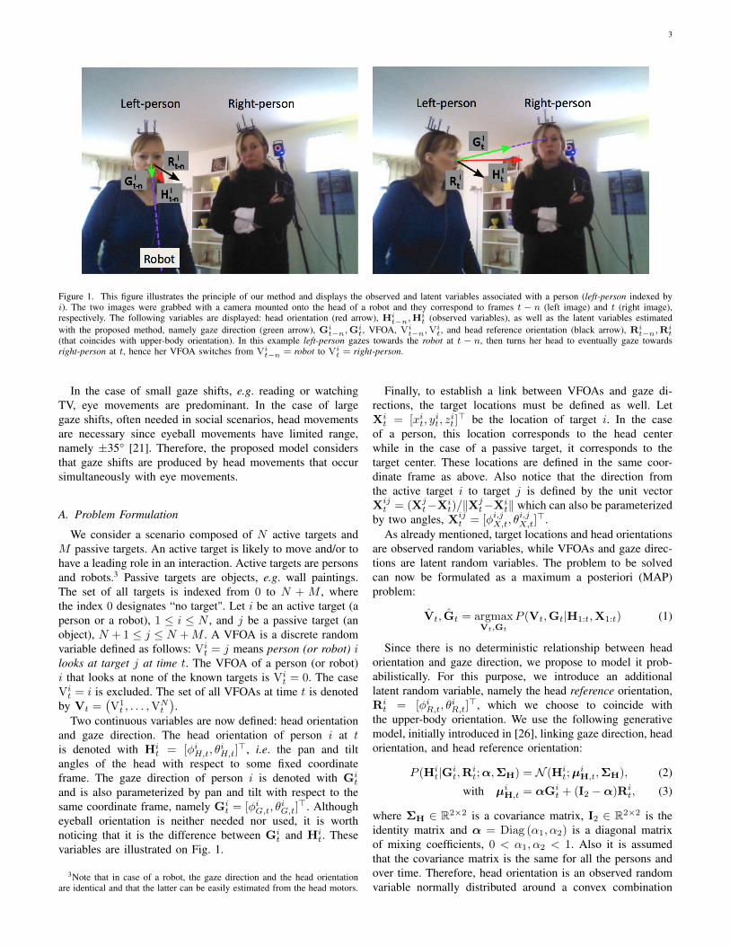
The Vernissage scenario can be briefly described as follows,e.g. Fig. 3: there are three wall paintings, namely the passivetargets denoted with o1, o2, and o3 (M = 3); two persons,denoted left person (left-p) and right person (right-p), interactwith the robot, hence N = 3. The robot plays the role ofan art guide, describing the paintings and asking questionsto the two persons in front of him. Each recording is splitinto two roughly equal parts. The first part is dedicated topainting explanation, with a one-way interaction. The secondpart consists of a quiz, thus illustrating a dialog between thetwo participants and the robot, most of the time concerningthe paintings.

Figure 3. The Vernissage setup. Left: Global view of an “exhibition" showingwall paintings, two participants, i.e. left-p and right-p, and the NAO robot.Right: Top view of the room showing the Vernissage layout.

The scene was recorded with a camera embedded intothe robot head and with a VICON motion capture systemconsisting of a network of infrared cameras, placed onto the

8

walls, and of optical markers, placed onto the robot and peopleheads. Both were recorded at 25 frames per second (fps).There is a total of ten recordings, each lasting ten minutes. TheVICON system provided accurate estimates of head positions,X1:T and head orientations, H1:T . Head positions and headorientations were also estimated using from the RGB imagesgathered with the camera embedded into the robot head. TheRGB images are processed as follows. We use the OpenCVversion of [36] to detect faces and their bounding boxes whichare then tracked over time using [37]. Next, we extract HOGdescriptors from each bounding box and apply a head-poseestimator, e.g. [38]. This yields H1:T . The 3D head positions,X1:T , can be estimated using the line of sight through theface center and the bounding-box size, which provides a roughestimate of the depth along the line of sight.

In the remaining of this paper, X1:T and H1:T are referredto as Vicon Data; X1:T and H1:T as RGB Data. Because thewhole setup was carefully calibrated, both Vicon and RGBData are represented in the same coordinate frame.

In all our experiments we assumed that the passive targetsare static and their positions are provided in advance. Theposition of the robot itself is also known in advance and onecan easily estimate the orientation of the robot head frommotor readings. Finally, the VFOAs of the participants weremanually annotated in all the frames of all the recordings.

B. The LAEO Dataset

The LAEO dataset [4] is an extension of the TVHID (TVHuman Interaction Dataset) [39]. It consists of 300 videosextracted from TV shows. At least two actors appear in eachvideo engaged in four human-human interactions: handshake,highfive, hug, and kiss. There are 50 videos for each interac-tion and 100 videos with no interaction. The videos have beengrabbed at 25 fps and each video lasts from five seconds totwenty-five seconds. LAEO is further annotated, namely someof these videos are split into shots which are separated by cuts.There are 443 shots in total which are manually annotatedwhenever two persons look at each other, [4].

While there is no passive target in this dataset (M = 0),the number of active targets (N ) corresponds to the numberof persons in each shot. In practice N varies from one toeight persons. All the faces in the dataset are annotated witha bounding box and with a coarse head-orientation label:frontal-right, frontal-left, profile-right, profile-left, backward.As with Vernissage, we use the bounding-box center and sizeto estimate the 3D coordinates of the heads, X1:T . We alsoassigned a yaw value to each one of the five coarse headorientations, H1:T . We also computed finer head orientations,H1:T , using [38].

C. Algorithmic Details

The inference procedure is summarized in Algorithm 1.This is basically an iterative filtering procedure. The updatestep consists of applying the recursive relationship, derived inSection IV, to µijt , Σij

t and cijt , using µijkt , Σijkt and cijkt−1,t as

intermediate variables. The VFOA is chosen using MAP, givenobservations up to the current frame, and the gaze direction is

the mean of the filtered distribution (the first two componentsof µijt are indeed the mean for the pan and tilt gaze angles).

Algorithm 1 Inference1: procedure GAZEANDVFOA2: X1,H1 ← GETOBSERVATIONS(time = 1)3: c1,µ1,Σ1 ← INITIALIZATION(H1,X1)4: Vi

1 ← argmaxj cij1

5: Gi1 ← µij1 [1..2]

6: for t = 2..T do7: Xt,Ht ← GETOBSERVATIONS(time = t)8: ct,µt,Σt ← UPDATE(Ht,Xt, ct−1,µt−1,Σt−1)

9: Vit ← argmaxj c

ijt

10: Git ← µijt [1..2]

11: return V1:T ,G1:T

Let’s now describe the initialization procedure used byAlgorithm 2. In a probabilistic framework, parameter intial-ization is generally addressed by defining an initial distri-bution, e.g. P (L1|V1). Here, we did not explicitly definesuch a distribution. Initialization is based on the fact that,with repeated similar observation inputs, the algorithm reachesa steady-state. The initialization algorithm uses a repeatedupdate method with initial observation to provide an estimateof gaze and of reference directions. Consequently, the initialfiltering distribution P (L1,V1|H1,X1) is implicitly definedas the expected stationary state.

Algorithm 2 Initialization1: procedure INITIALIZATION(H1,X1)2: µin ← [H1; 0; H1; 0]3: Σin ← I4: cin ← 1

N+M (Uniform)5: while Not Convergence do6: cin,µin,Σin ← UPDATE(H1,X1, cin,µin,Σin)

7: return cin,µin,Σin

D. Algorithm Complexity

The computational complexity of Algorithm 1 is

C = T (CO + CU ) + TICU , (52)

where T is the number of frames in a test video, TI is thenumber of iterations needed by the Algorithm 2 (initializa-tion) to converge, CO is the computational complexity ofGETOBSERVATION and CU is the computational complexityof UPDATE. The complexity of one iteration of Algorithm 1is CO + CU . CO depends on face detection and head poseestimation algorithms. Hence we concentrate on CU . FromSection IV one sees that the following values need to becomputed: P (Hi

t|Vit = j,Vi

t−1 = k,H1:t−1,X1:t−1), cijkt−1,t,µijkt , Σijk

t , and then cijt , µijt and Σijt , for each active target

i, and for each combination of targets j and k different fromi. There are N possible values for i and (N + M) possiblevalues for j and k. Then,

CU = K ×N(N +M)2, (53)

9

where K is a factor whose complexity can be estimated asfollows. The most time-consuming part is the Kalman Filteralgorithm used to estimate µijkt and Σijk

t from µikt and Σikt .

These calculations are dominated by several 8×8 and 2×8matrix inversions and multiplications. By neglecting scalarmultiplications and matrix additions, and by denoting withCKF the complexity of the Kalman filter, we obtain thatK ≈ CKF and hence CU ≈ CKF ×N(N +M)2.

VII. EXPERIMENTAL RESULTS

A. Vernissage Dataset

We applied the same experimental protocol to the Vicon andRGB data. We used a leave-one-video-out strategy for training.The test is performed on the left out video. We used the framerecognition rate (FRR) metrics to quantitatively evaluate themethods. FRR computes the percentage of frames for whichthe VFOA is correctly estimated. One should note howeverthat the ground-truth VFOAs were obtained by manuallyannotating each frame in the data. This is subject to errorssince the annotator has to associate a target with each person.

The VFOA transition probabilities and the model parameterswere estimated using the learning method described in Sec-tion V. Appendix B provides the formulas used for estimatingthe VFOA transition probabilities given the annotated data.Notice that the fifteen transitions probabilities thus estimatedare identical for both data, Vicon and RGB.

The Gaussian parameters, i.e. (35), were estimated usingthe EM algorithm of Section V-B. This learning procedurerequires head-pose estimates as well as the targets locations,estimated as just explained. Since these estimates are differentfor the two kinds of data (Vicon and RGB) we carried outthe learning process twice, with the Vicon data and with theRGB data. The EM algorithm needs initialization. The initialparameter values for α and β are α0 = β0 = Diag (0.5, 0.5).Matrices ΣH and ΓL defined in (20) are initialized withisotropic covariances: Σ0

H = σI2, Γ0G = Γ0

G= γI2, and

Γ0R = Γ0

R= ηI2 with σ = 15, γ = 5, and η = 0.5. In

particular, this initialization is consistent with (12). In practicewe noticed that the covariances estimated by training remainconsistent with (12).

B. Results with Vicon Data

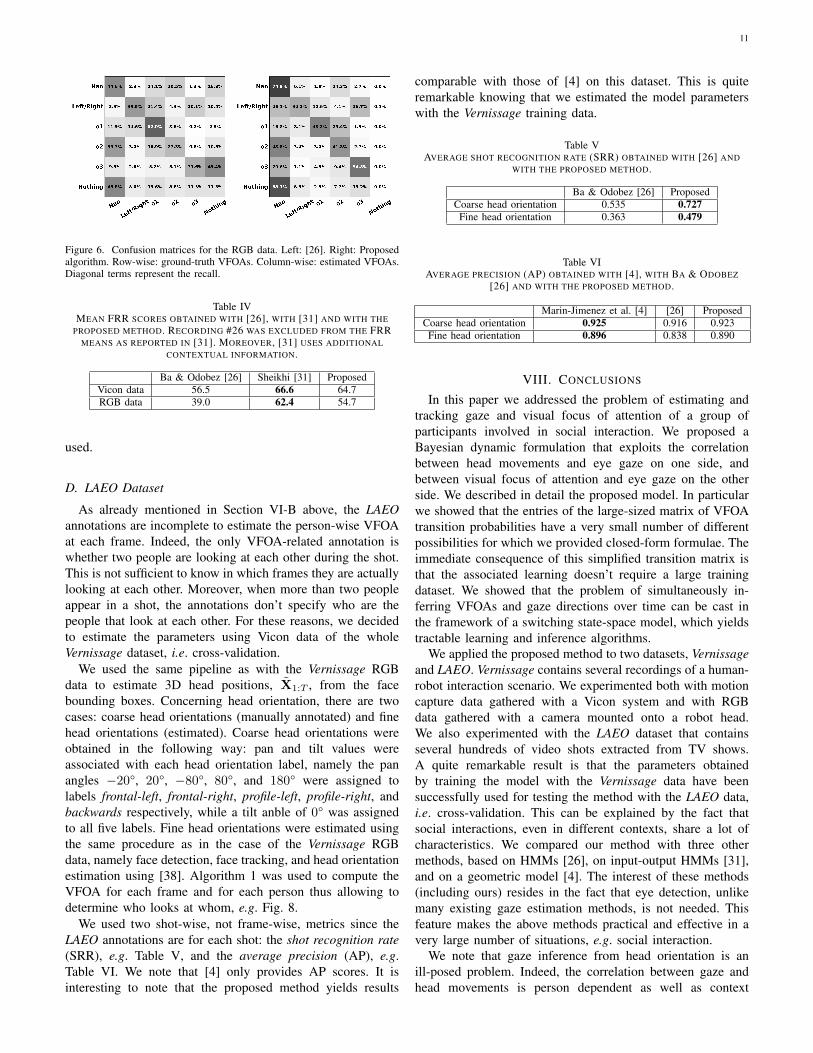
The FRR of the estimated VFOAs for the Vicon data aresummarized in Table I. A few examples are shown in Figure 5.The FRR score varies between 28.3% and 74.4% for [26]and between 43.1% and 79.8% for the proposed method.Notice that high scores are obtained by both methods forrecording #27. Similarly, low scores are obtained for recording#26. Since both methods assume that head motions and gazeshifts occur synchronously, an explanation could be that thishypothesis is only valid for some of the participants. Theconfusion matrices for VFOA classification using Vicon dataare given in Figure 4. There are a few similarities betweenthe results obtained with the two methods. In particular, wallpainting #o2 stands just behind Nao and both methods don’talways discriminate between these two targets. In addition,the head of one of the persons is often aligned with painting

Table IFRR SCORES OF THE ESTIMATED VFOAS FOR THE VICON DATA FOR THE

LEFT AND RIGHT PERSONS (LEFT-P AND RIGHT-P).

Recording Ba & Odobez [26] Proposedleft-p right-p left-p right-p

09 51.6 65.1 59.8 61.410 64.3 74.4 76.5 65.012 53.5 67.6 61.6 63.215 67.1 46.2 64.8 67.618 37.5 28.3 62.0 53.719 56.7 45.4 54.5 60.424 44.9 49.0 59.7 54.726 40.3 32.9 43.6 43.127 65.8 72.0 79.8 78.330 69.1 49.1 72.0 63.9

Mean 54.5 62.6

Figure 4. Confusion matrices for the Vicon data. Left: [26]. Right: Proposedalgorithm. Row-wise: ground-truth VFOAs. Column-wise: estimated VFOAs.Diagonal terms represent the recall.

#o1 from the viewpoint of the other person. A similar remarkholds for painting #o3. As a consequence both methods oftenconfuse the VFOA in these cases. This can be seen in the thirdimage of Figure 5. Indeed, it is difficult to estimate whetherthe left person (left-p) looks at #o1 or at right-p.

Finally, both methods have problems with recognizing theVFOA “nothing” or gaze aversion (Vi

t = 0). We proposethe following explanation: the targets are widespread in thescene, hence it is likely that an acceptable target lies in mostof the gaze directions. Moreover, Nao is centrally positioned,therefore the head orientation used to look at Nao is similar tothe resting head orientation used for gaze aversion. However,in [26] the reference head orientation is fixed and poorly suitedfor dynamic head-to-gaze mapping, hence the high error rateon painting #o3. Our method favors the selection of a target,either active or passive, over the no target (nothing) case.

C. Results with RGB Data

The RGB images were processed as described in sec-tion VI-A above in order to obtain head orientations, H1:T ,and 3D head positions, X1:T . Table II shows the accuracyof these measurements (in degrees and in centimeters), whencompared with the ground truth provided by the Vicon motioncapture system. As it can be seen, while the head orientationestimates are quite accurate, the error in estimating the headpositions can be as large as 0.8 m for participants lying inbetween 1.5 m and 2.5 m in front of a robot, e.g. recordings#19 and #24. In particular this error increases as a participantis farther away from the robot. In these cases, the bounding

10

Figure 5. Results obtained with the proposed method on Vicon data. Gaze directions are shown with green arrows, head reference directions with dark-greyarrows and observed head directions with red arrows. The ground-truth VFOA is shown with a black circle. The top row displays the image of the robot-headcamera. Top views of the room show results obtained for the left-p (middle row) and for the right-p (bottom row). In the last example the left-p gazes at“nothing".

box is larger than it should be and hence the head position is,on an average, one meter closer than the true position. Theserelatively large errors in 3D head position affect the overallbehavior of the algorithm.

The FRR scores obtained with the RGB data are shown inTable III. As expected the loss in accuracy is correlated withthe head position error: the results obtained with recordings#09 and #30 are close to the ones obtained with the Vicondata, whereas there is a significant loss in accuracy for theother recordings. The loss is notable for [26] in the case ofthe right person (right-p) for the recordings #12, #18 and #27.The confusion matrices obtained with the RGB data are shown

Table IIMEAN ERROR FOR HEAD POSE ESTIMATIONS FROM RGB DATA, FOR THELEFT PERSON (LEFT-P) AND THE RIGHT PERSON (RIGHT-P). THE ERRORSIN HEAD POSITION (CENTIMETERS) AND ORIENTATION (DEGREES) ARE

COMPUTED WITH RESPECT TO VALUES PROVIDED BY THE MOTIONCAPTURE SYSTEM.

Video Position error (cm) Pan error Tilt errorleft-p right-p left-p right-p left-p right-p

09 18.1 20.8 4.4° 4.8° 3.7° 3.2°12 35.7 41.5 4.8° 5.5° 2.6° 3.8°18 36.9 12.8 6.8° 3.7° 5.8° 2.5°19 86.0 87.4 4.0° 5.8° 2.7° 3.7°24 86.5 73.9 3.3° 3.5° 2.8° 2.7°26 50.2 56.9 7.4° 9.0° 4.1° 5.2°27 64.5 58.3 4.1° 5.8° 3.2° 4.4°30 16.7 13.3 2.8° 2.9° 1.8° 2.7°

Mean 46.4 5.0° 3.3°

on Fig. 6.In the case of RGB data, the comparison between our

method and the method of [31] is biased by the use of differenthead orientation and 3D head position estimators. Indeed,the RGB data results reported in [31] were obtained withunpublished methods for estimating head orientations and 3Dhead positions, and for head tracking. Moreover, [31] usescross-modal information, namely the speaker identity basedon the audio track (one of the participants or the robot) aswell as the identity of the object of interest. We also notethat [31] reports mean FRR values obtained over all thetest recordings, instead of an FRR value for each recording.Table IV summarizes a comparison between the average FRRobtained with our method, with [26], and with [31]. Ourmethod yields a similar FRR score as [31] using the Vicondata (first row) in which case the same head pose inputs are

Table IIIFRR SCORES OF THE ESTIMATED VFOAS OBTAINED WITH [26] ANDWITH THE PROPOSED METHOD FOR THE RGB DATA. THE LAST TWO

COLUMNS SHOW THE 3D HEAD POSITION ERRORS OF TABLE II.

Video Ba & Odobez [26] Proposed Head pos. errorleft-p right-p left-p right-p left-p right-p

09 50.3 59.8 58.1 55.9 18.1 20.812 54.2 14.8 59.0 46.5 35.7 41.518 39.0 16.1 64.2 33.1 36.9 12.827 38.2 17.1 53.3 55.1 64.5 58.330 61.6 44.6 54.7 66.6 16.7 13.3

Mean 39.0 54.7

11

Figure 6. Confusion matrices for the RGB data. Left: [26]. Right: Proposedalgorithm. Row-wise: ground-truth VFOAs. Column-wise: estimated VFOAs.Diagonal terms represent the recall.

Table IVMEAN FRR SCORES OBTAINED WITH [26], WITH [31] AND WITH THE

PROPOSED METHOD. RECORDING #26 WAS EXCLUDED FROM THE FRRMEANS AS REPORTED IN [31]. MOREOVER, [31] USES ADDITIONAL

CONTEXTUAL INFORMATION.

Ba & Odobez [26] Sheikhi [31] ProposedVicon data 56.5 66.6 64.7RGB data 39.0 62.4 54.7

used.

D. LAEO Dataset

As already mentioned in Section VI-B above, the LAEOannotations are incomplete to estimate the person-wise VFOAat each frame. Indeed, the only VFOA-related annotation iswhether two people are looking at each other during the shot.This is not sufficient to know in which frames they are actuallylooking at each other. Moreover, when more than two peopleappear in a shot, the annotations don’t specify who are thepeople that look at each other. For these reasons, we decidedto estimate the parameters using Vicon data of the wholeVernissage dataset, i.e. cross-validation.

We used the same pipeline as with the Vernissage RGBdata to estimate 3D head positions, X1:T , from the facebounding boxes. Concerning head orientation, there are twocases: coarse head orientations (manually annotated) and finehead orientations (estimated). Coarse head orientations wereobtained in the following way: pan and tilt values wereassociated with each head orientation label, namely the panangles −20°, 20°, −80°, 80°, and 180° were assigned tolabels frontal-left, frontal-right, profile-left, profile-right, andbackwards respectively, while a tilt anble of 0° was assignedto all five labels. Fine head orientations were estimated usingthe same procedure as in the case of the Vernissage RGBdata, namely face detection, face tracking, and head orientationestimation using [38]. Algorithm 1 was used to compute theVFOA for each frame and for each person thus allowing todetermine who looks at whom, e.g. Fig. 8.

We used two shot-wise, not frame-wise, metrics since theLAEO annotations are for each shot: the shot recognition rate(SRR), e.g. Table V, and the average precision (AP), e.g.Table VI. We note that [4] only provides AP scores. It isinteresting to note that the proposed method yields results

comparable with those of [4] on this dataset. This is quiteremarkable knowing that we estimated the model parameterswith the Vernissage training data.

Table VAVERAGE SHOT RECOGNITION RATE (SRR) OBTAINED WITH [26] AND

WITH THE PROPOSED METHOD.

Ba & Odobez [26] ProposedCoarse head orientation 0.535 0.727Fine head orientation 0.363 0.479

Table VIAVERAGE PRECISION (AP) OBTAINED WITH [4], WITH BA & ODOBEZ

[26] AND WITH THE PROPOSED METHOD.

Marin-Jimenez et al. [4] [26] ProposedCoarse head orientation 0.925 0.916 0.923Fine head orientation 0.896 0.838 0.890

VIII. CONCLUSIONS

In this paper we addressed the problem of estimating andtracking gaze and visual focus of attention of a group ofparticipants involved in social interaction. We proposed aBayesian dynamic formulation that exploits the correlationbetween head movements and eye gaze on one side, andbetween visual focus of attention and eye gaze on the otherside. We described in detail the proposed model. In particularwe showed that the entries of the large-sized matrix of VFOAtransition probabilities have a very small number of differentpossibilities for which we provided closed-form formulae. Theimmediate consequence of this simplified transition matrix isthat the associated learning doesn’t require a large trainingdataset. We showed that the problem of simultaneously in-ferring VFOAs and gaze directions over time can be cast inthe framework of a switching state-space model, which yieldstractable learning and inference algorithms.

We applied the proposed method to two datasets, Vernissageand LAEO. Vernissage contains several recordings of a human-robot interaction scenario. We experimented both with motioncapture data gathered with a Vicon system and with RGBdata gathered with a camera mounted onto a robot head.We also experimented with the LAEO dataset that containsseveral hundreds of video shots extracted from TV shows.A quite remarkable result is that the parameters obtainedby training the model with the Vernissage data have beensuccessfully used for testing the method with the LAEO data,i.e. cross-validation. This can be explained by the fact thatsocial interactions, even in different contexts, share a lot ofcharacteristics. We compared our method with three othermethods, based on HMMs [26], on input-output HMMs [31],and on a geometric model [4]. The interest of these methods(including ours) resides in the fact that eye detection, unlikemany existing gaze estimation methods, is not needed. Thisfeature makes the above methods practical and effective in avery large number of situations, e.g. social interaction.

We note that gaze inference from head orientation is anill-posed problem. Indeed, the correlation between gaze andhead movements is person dependent as well as context

12

Figure 7. Results obtained with the proposed method on RGB data. Gaze directions are shown with green arrows, head reference directions with dark-greyarrows and observed head directions with red arrows. The ground-truth VFOA is shown with a black circle. The top row displays the image of the robot-headcamera. Top views of the room show results obtained for the left person (left-p, middle row) and the right person (right-p, bottom row).

Figure 8. This figure shows some results obtained with the LAEO dataset. The top row shows results obtained with coarse head orientation and the bottomrow shows results obtained with fine head orientation. Head orientations are shown with red arrows. The algorithm infers gaze directions (green arrows) andVFOAs (blue circles). People looking at each others are shown with a dashed blue line.

dependent. It is however important to detect gaze wheneverthe eyes cannot be reliably extracted from images and properlyanalyzed. We proposed to solve the problem based on thefact that alignments often occur between gaze directions anda finite number of targets, which is a sensible assumption inpractice.

Contextual information could considerably improve the re-sults. Indeed, additional information such as speaker recogni-tion (as in [31]), speaker localization [40], speech recognition,or speech-turn detection [41] may be used to learn VFOAtransitions in multi-party multimodal dialog systems.

In the future we plan to investigate discriminative methodsbased on neural network architectures for inferring gaze direc-

tions from head orientations and from contextual information.For example one could train a deep learning network frominput-output pairs of head pose and visual focus of attention.For this purpose, one can combine a multiple-camera system,to accurately detect the eyes of several participants and to esti-mate their head poses, with a microphone-array and associatedalgorithms to infer speaker and speech information.

APPENDIX AVFOA TRANSITION PROBABILITIES

Using the notations introduced in section III-C, let i, 1 ≤i ≤ N , be an active target. In section III-C we showed that in

13

practice the probability transition matrix has up to 15 differententries. For completeness, these entries are listed below.• The VFOA of i at t−1 is neither an active nor a passive

target (k = 0):

p1 =P (Vit = 0|Vi

t−1 = 0)

p2 =P (Vit = j|Vi

t−1 = 0)

• The VFOA of i at t − 1 is a passive target (N < k ≤N +M ):

p3 =P (Vit = 0|Vi

t−1 = k)

p4 =P (Vit = k|Vi

t−1 = k)

p5 =P (Vit = j|Vi

t−1 = k)

• The VFOA of i at t − 1 is an active target (1 ≤ k ≤N, k 6= i):

p6 =P (Vit = 0|Vi

t−1 = k,Vkt−1 = 0)

p7 =P (Vit = k|Vi

t−1 = k,Vkt−1 = 0)

p8 =P (Vit = j|Vi

t−1 = k,Vkt−1 = 0)

p9 =P (Vit = 0|Vi

t−1 = k,Vkt−1 = i)

p10 =P (Vit = k|Vi

t−1 = k,Vkt−1 = i)

p11 =P (Vit = j|Vi

t−1 = k,Vkt−1 = i)

p12 =P (Vit = 0|Vi

t−1 = k,Vkt−1 = l)

p13 =P (Vit = k|Vi

t−1 = k,Vkt−1 = l)

p14 =P (Vit = l|Vi

t−1 = k,Vkt−1 = l)

p15 =P (Vit = j|Vi

t−1 = k,Vkt−1 = l)

APPENDIX BVFOA LEARNING

This appendix provides the formulae allowing to estimatethe 15 transitions probabilities as explained in section V-A.

p1 =

Q∑q=1

Nq∑i=2

Tq∑t=2

δ0(Vq,it )δ0(Vq,i

t−1)

Q∑q=1

Nq∑i=2

Tq∑t=2

δ0(Vq,it−1)

p2 =

Q∑q=1

Nq∑i=2

Tq∑t=2

∑j 6=i

δj(Vq,it )δ0(Vq,i

t−1)

Q∑q=1

Nq∑i=2

Tq∑t=2

δ0(Vq,it−1)

p3 =

Q∑q=1

Nq∑i=2

Tq∑t=2

Nq+Mq∑k=Nq+1

δ0(Vq,it )δk(Vq,i

t−1)

Q∑q=1

Nq∑i=2

Tq∑t=2

Nq+Mq∑k=Nq+1

δk(Vq,it−1)

p4 =

Q∑q=1

Nq∑i=2

Tq∑t=2

Nq+Mq∑k=Nq+1

δk(Vq,it )δk(Vq,i

t−1)

Q∑q=1

Nq∑i=2

Tq∑t=2

Nq+Mq∑k=Nq+1

δk(Vq,it−1)

p5 =

Q∑q=1

Nq∑i=2

Tq∑t=2

Nq+Mq∑k=Nq+1

∑j 6=i,k

δj(Vq,it )δk(Vq,i

t−1)

Q∑q=1

Nq∑i=2

Tq∑t=2

Nq+Mq∑k=Nq+1

δk(Vq,it−1)

p6 =

Q∑q=1

Nq∑i=2

Tq∑t=2

Nq∑k=1k 6=i

δ0(Vq,it )δk(Vq,i

t−1)δ0(Vq,kt−1)

Q∑q=1

Nq∑i=2

Tq∑t=2

Nq∑k=1k 6=i

δk(Vq,it−1)δ0(Vq,k

t−1)

p7 =

Q∑q=1

Nq∑i=2

Tq∑t=2

Nq∑k=1k 6=i

δk(Vq,it )δk(Vq,i

t−1)δ0(Vq,kt−1)

Q∑q=1

Nq∑i=2

Tq∑t=2

Nq∑k=1k 6=i

δk(Vq,it−1)δ0(Vq,k

t−1)

p8 =

Q∑q=1

Nq∑i=2

Tq∑t=2

Nq∑k=1k 6=i

∑j 6=i,k

δj(Vq,it )δk(Vq,i

t−1)δ0(Vq,kt−1)

Q∑q=1

Nq∑i=2

Tq∑t=2

Nq∑k=1k 6=i

δk(Vq,it−1)δ0(Vq,k

t−1)

p9 =

Q∑q=1

Nq∑i=2

Tq∑t=2

Nq∑k=1k 6=i

δ0(Vq,it )δk(Vq,i

t−1)δi(Vq,kt−1)

Q∑q=1

Nq∑i=2

Tq∑t=2

Nq∑k=1k 6=i

δk(Vq,it−1)δi(V

q,kt−1)

p10 =

Q∑q=1

Nq∑i=2

Tq∑t=2

Nq∑k=1k 6=i

δk(Vq,it )δk(Vq,i

t−1)δi(Vq,kt−1)

Q∑q=1

Nq∑i=2

Tq∑t=2

Nq∑k=1k 6=i

δk(Vq,it−1)δi(V

q,kt−1)

14

p11 =

Q∑q=1

Nq∑i=2

Tq∑t=2

Nq∑k=1k 6=i

∑j 6=i,k

δj(Vq,it )δk(Vq,i

t−1)δi(Vq,kt−1)

Q∑q=1

Nq∑i=2

Tq∑t=2

Nq∑k=1k 6=i

δk(Vq,it−1)δi(V

q,kt−1)

p12 =

Q∑q=1

Nq∑i=2

Tq∑t=2

Nq∑k=1k 6=i

∑l 6=i,k

δ0(Vq,it )δk(Vq,i

t−1)δl(Vq,kt−1)

Q∑q=1

Nq∑i=2

Tq∑t=2

Nq∑k=1k 6=i

∑l 6=i,k

δk(Vq,it−1)δl(V

q,kt−1)

p13 =

Q∑q=1

Nq∑i=2

Tq∑t=2

Nq∑k=1k 6=i

∑l 6=i,k

δk(Vq,it )δk(Vq,i

t−1)δl(Vq,kt−1)

Q∑q=1

Nq∑i=2

Tq∑t=2

Nq∑k=1k 6=i

∑l 6=i,k

δk(Vq,it−1)δl(V

q,kt−1)

p14 =

Q∑q=1

Nq∑i=2

Tq∑t=2

Nq∑k=1k 6=i

∑l 6=i,k

δl(Vq,it )δk(Vq,i

t−1)δl(Vq,kt−1)

Q∑q=1

Nq∑i=2

Tq∑t=2

Nq∑k=1k 6=i

∑l 6=i,k

δk(Vq,it−1)δl(V

q,kt−1)

p15 =

Q∑q=1

Nq∑i=2

Tq∑t=2

Nq∑k=1k 6=i

∑l 6=i,k

∑j 6=i,k,l

δj(Vq,it )δk(Vq,i

t−1)δl(Vq,kt−1)

Q∑q=1

Nq∑i=2

Tq∑t=2

Nq∑k=1k 6=i

∑l 6=i,k

δk(Vq,it−1)δl(V

q,kt−1)

ACKNOWLEDGMENTS

The authors would like to thank Vincent Drouard for hisvaluable expertise in head pose estimation and tracking.

REFERENCES

[1] E. G. Freedman and D. L. Sparks, “Eye-head coordination during head-unrestrained gaze shifts in rhesus monkeys,” Journal of Neurophysiol-ogy, 1997.

[2] E. G. Freedman, “Coordination of the eyes and head during visualorienting,” Experimental Brain Research, vol. 190, 2008.

[3] D. B. Jayagopi et al., “The vernissage corpus: A multimodal human-robot-interaction dataset,” IDIAP, Tech. Rep., 2012.

[4] M. J. Marin-Jimenez, A. Zisserman, M. Eichner, and V. Ferrari, “De-tecting people looking at each other in videos,” International Journal ofComputer Vision, vol. 106, 2014.

[5] L. H. Yu and M. Eizenman, “A new methodology for determining point-of-gaze in head-mounted eye tracking systems,” IEEE Transactions onBiomedical Engineering, vol. 51, Oct 2004.

[6] T. Toyama, T. Kieninger, F. Shafait, and A. Dengel, “Gaze guided objectrecognition using a head-mounted eye tracker,” in Proceedings of theETRA Symposium, 2012.

[7] A. K. A. Hong, J. Pelz, and J. Cockburn, “Lightweight, low-cost, side-mounted mobile eye tracking system,” in IEEE WNYIPW, 2012.

[8] K. Kurzhals, M. Hlawatsch, C. Seeger, and D. Weiskopf, “Visualanalytics for mobile eye tracking,” IEEE Transactions on Visualizationand Computer Graphics, vol. 23, no. 1, pp. 301–310, Jan 2017.

[9] P. Smith, M. Shah, and N. Da Vitoria Lobo, “Determining drivervisual attention with one camera,” IEEE Transactions on IntelligentTransportation Systems, vol. 4, 2003.

[10] K. Krafka, A. Khosla, P. Kellnhofer, H. Kannan, S. Bhandarkar, W. Ma-tusik, and A. Torralba, “Eye tracking for everyone,” in IEEE CVPR, June2016.

[11] Y. Matsumoto, T. Ogasawara, and A. Zelinsky, “Behavior recognitionbased on head pose and gaze direction measurement,” in IEEE IROS,vol. 3, 2000.

[12] T. Ohno and N. Mukawa, “A free-head, simple calibration, gaze trackingsystem that enables gaze-based interaction,” in Proceedings of the ETRASymposium. ACM, 2004.

[13] F. Lu, Y. Sugano, T. Okabe, and Y. Sato, “Adaptive linear regressionfor appearance-based gaze estimation,” IEEE Transactions on PatternAnalysis and Machine Intelligence, vol. 36, Oct 2014.

[14] F. Lu, T. Okabe, Y. Sugano, and Y. Sato, “Learning gaze biases withhead motion for head pose-free gaze estimation,” Image and VisionComputing, vol. 32, 2014.

[15] E. Murphy-Chutorian and M. Trivedi, “Head pose estimation in com-puter vision: A survey,” IEEE Transactions on Pattern Analysis andMachine Intelligence, vol. 31, 2009.

[16] X. Zabulis, T. Sarmis, and A. A. Argyros, “3D head pose estimationfrom multiple distant views,” in BMVC, 2009.

[17] I. Chamveha, Y. Sugano, D. Sugimura, T. Siriteerakul, T. Okabe, Y. Sato,and A. Sugimoto, “Head direction estimation from low resolution imageswith scene adaptation,” Computer Vision and Image Understanding, vol.117, 2013.

[18] A. K. Rajagopal, R. Subramanian, E. Ricci, R. L. Vieriu, O. Lanz, andN. Sebe, “Exploring transfer learning approaches for head pose classi-fication from multi-view surveillance images,” International Journal ofComputer Vision, vol. 109, 2014.

[19] Y. Yan, E. Ricci, R. Subramanian, G. Liu, O. Lanz, and N. Sebe, “Amulti-task learning framework for head pose estimation under target mo-tion,” IEEE Transactions on Pattern Analysis and Machine Intelligence,vol. 38, 2016.

[20] Z. Qin and C. R. Shelton, “Social grouping for multi-target tracking andhead pose estimation in video,” IEEE Transactions on Pattern Analysisand Machine Intelligence, vol. 38, 2016.

[21] J. S. Stahl, “Amplitude of human head movements associated withhorizontal saccades,” Experimental Brain Research, vol. 126, 1999.

[22] H. H. Goossens and A. Van Opstal, “Human eye-head coordination intwo dimensions under different sensorimotor conditions,” ExperimentalBrain Research, vol. 114, 1997.

[23] R. Stiefelhagen and J. Zhu, “Head orientation and gaze direction inmeetings,” in Human Factors in Computing Systems, 2002.

[24] P. Lanillos, J. F. Ferreira, and J. Dias, “A bayesian hierarchy for robustgaze estimation in human-robot interaction,” International Journal ofApproximate Reasoning, vol. 87, 05 2017.

[25] S. Asteriadis, K. Karpouzis, and S. Kollias, “Visual focus of attentionin non-calibrated environments using gaze estimation,” InternationalJournal of Computer Vision, vol. 107, 2014.

[26] S. Ba and J.-M. Odobez, “Recognizing visual focus of attention fromhead pose in natural meetings,” IEEE Transactions on System Men andCybernetics. Part B., 2009.

[27] S. Sheikhi and J.-M. Odobez, “Recognizing the visual focus of atten-tion for human robot interaction,” in Human Behavior UnderstandingWorkshop, 2012.

[28] Z. Yucel, A. A. Salah, C. Mericli, T. Mericli, R. Valenti, and T. Gevers,“Joint attention by gaze interpolation and saliency,” IEEE Transactionson System Men and Cybernetics. Part B., 2013.

[29] K. Otsuka, J. Yamato, and Y. Takemae, “Conversation scene analysiswith dynamic bayesian network based on visual head tracking,” in IEEEICME, 2006.

[30] S. Duffner and C. Garcia, “Visual focus of attention estimation withunsupervised incremental learning,” IEEE Transactions on Circuits andSystems for Video Technology, 2015.

[31] S. Sheikhi and J.-M. Odobez, “Combining dynamic head pose–gazemapping with the robot conversational state for attention recognition inhuman–robot interactions,” Pattern Recognition Letters, vol. 66, 2015.

[32] B. Massé, S. Ba, and R. Horaud, “Simultaneous estimation of gaze direc-tion and visual focus of attention for multi-person-to-robot interaction,”in IEEE ICME, Seattle, WA, Jul. 2016.

15

[33] K. P. Murphy, “Switching Kalman filters,” UC Berkeley, Tech. Rep.,1998.

[34] D. Simon, “Kalman filtering with state constraints: a survey of linearand nonlinear algorithms,” Control Theory Applications, IET, 2010.

[35] C. M. Bishop, Pattern Recognition and Machine Learning. Springer-Verlag, 2006.

[36] P. Viola and M. Jones, “Rapid object detection using a boosted cascadeof simple features,” in IEEE CVPR, vol. 1, 2001.

[37] S.-H. Bae and K.-J. Yoon, “Robust online multi-object tracking basedon tracklet confidence and online discriminative appearance learning,”in IEEE CVPR, 2014.

[38] V. Drouard, R. Horaud, A. Deleforge, S. Ba, and G. Evangelidis,“Robust head-pose estimation based on partially-latent mixture of linearregressions,” IEEE Transactions on Image Processing, vol. 26, Jan.2017.

[39] A. Patron-Perez, M. Marszałek, A. Zisserman, and I. D. Reid, “Highfive: Recognising human interactions in TV shows,” in British MachineVision Conference, 2010.

[40] X. Li, L. Girin, R. Horaud, and S. Gannot, “Multiple-speaker localizationbased on direct-path features and likelihood maximization with spatialsparsity regularization,” IEEE/ACM Transactions on Audio, Speech, andLanguage Processing, vol. 25, no. 10, pp. 1997–2012, Oct 2017.

[41] I. Gebru, S. Ba, X. Li, and R. Horaud, “Audio-visual speaker diarizationbased on spatiotemporal bayesian fusion,” IEEE Transactions on PatternAnalysis and Machine Intelligence, 2017.

Benoit Massé received the M.Eng. degree in appliedmathematics and computer science from ENSIMAG,Institut National Polytechnique de Grenoble, France,in 2013, and the M.Sc. degree in graphics, vision androbotics from Université Joseph Fourier, Grenoble,France, in 2014. Currently he is a PhD student inthe PERCEPTION team at INRIA Grenoble Rhone-Alpes. His research interests include scene under-standing, machine learning and computer vision,with special emphasis on attention recognition forhuman-robot interaction.

Silèye Ba received the M.Sc. (2000) in appliedmathematics and signal processing from Universityof Dakar, Dakar, Senegal, and the M.Sc. (2002) inmathematics, computer vision, and machine learningfrom Ecole Normale Supérieure de Cachan, Paris,France. From 2003 to 2009 he was a PhD stu-dent and then a post-doctoral researcher at IDIAPResearch Institute, Martigny, Switzerland, where heworked on probabilistic models for object trackingand human activity recognition. From 2009 to 2013,he was a researcher at Telecom Bretagne, Brest,

France working on variational models for multi-modal geophysical dataprocessing. From 2013 to 2014 he worked at RN3D Innovation Lab, Marseille,France, as a research engineer, where he used computer vision and machinelearning principles and methods to develop human-computer interactionsoftware tools. From 2014 to 2016 he was a researcher in the PERCEPTIONteam at INRIA Grenoble Rhône-Alpes, working on machine learning andcomputer vision models for human-robot interaction. Since May 2016 he isa computer vision scientist with VideoStitch, Paris.

Radu Horaud received the B.Sc. degree in Electri-cal Engineering, the M.Sc. degree in Control Engi-neering, and the Ph.D. degree in Computer Sciencefrom the Institut National Polytechnique de Greno-ble, France. In 1982-1984 he was a post-doctoralfellow with the Artificial Intelligence Center, SRIInternational, Menlo Park, CA. Currently he holds aposition of director of research with INRIA Greno-ble Rhône-Alpes, where he is the founder and headof the PERCEPTION team. His research interestsinclude computer vision, machine learning, audio

signal processing, audiovisual analysis, and robotics. Radu Horaud and hiscollaborators received numerous best paper awards. He is an area editor ofthe Elsevier Computer Vision and Image Understanding, a member of theadvisory board of the Sage International Journal of Robotics Research, andan associate editor of the Kluwer International Journal of Computer Vision.He was program co-chair of IEEE ICCV’01 and of ACM ICMI’15. In 2013,Radu Horaud was awarded an ERC Advanced Grant for his project Visionand Hearing in Action (VHIA) and in 2017 he was awarded an ERC Proofof Concept Grant for this project VHIALab.