Eur. Phys. J. Plus (2021) 136:864 https://doi.org/10.1140/epjp/s13360-021-01849-3

Regular Art icle

Tracking droplets in soft granular flows with deeplearning techniques

Mihir Durve1,a , Fabio Bonaccorso1,2,3, Andrea Montessori2 ,Marco Lauricella2 , Adriano Tiribocchi2 , Sauro Succi1,2,4

1 Center for Life Nano- & Neuro-Science, Fondazione Istituto Italiano di Tecnologia (IIT), 00161 Rome, Italy2 Istituto per le Applicazioni del Calcolo CNR, via dei Taurini 19, Rome, Italy3 Department of Physics and INFN, University of Rome Tor Vergata, Via della Ricerca Scientifica 1,

00133 Rome, Italy4 Institute for Applied Computational Science, John A. Paulson School of Engineering and Applied Sciences,

Harvard University, Cambridge, USA

Received: 6 July 2021 / Accepted: 7 August 2021© The Author(s) 2021

Abstract The state-of-the-art deep learning-based object recognition YOLO algorithm andobject tracking DeepSORT algorithm are combined to analyze digital images from fluiddynamic simulations of multi-core emulsions and soft flowing crystals and to track mov-ing droplets within these complex flows. The YOLO network was trained to recognize thedroplets with synthetically prepared data, thereby bypassing the labor-intensive data acqui-sition process. In both applications, the trained YOLO + DeepSORT procedure performswith high accuracy on the real data from the fluid simulations, with low error levels in theinferred trajectories of the droplets and independently computed ground truth. Moreover,using commonly used desktop GPUs, the developed application is capable of analyzing dataat speeds that exceed the typical image acquisition rates of digital cameras (30 fps), openingthe interesting prospect of realizing a low-cost and practical tool to study systems with manymoving objects, mostly but not exclusively, biological ones. Besides its practical applica-tions, the procedure presented here marks the first step towards the automatic extraction ofeffective equations of motion of many-body soft flowing systems.

1 Introduction

Over the last decade, machine learning has taken the scientific world by storm and evenmore so the commercial one. Even though it is not all old gold that glitters [1], the potentialof machine learning to gain new insights into a variety of complex systems in science andsociety is unquestionably tantalizing [2,3].

Deep learning is a sub-field of machine learning specifically inspired by the structure andfunction of the human brain [4]. Its core consists of artificial neural networks that imitate theoperation of the human brain in data processing and decision making. In the actual digitalera, which generates an unprecedented amount of data (Big Data) in the form of images, text,and audio-video clips, deep learning techniques have proved capable of extracting relevantinformation and correlations [4], sometimes dramatically abating the amount of time required

a e-mail: mihirdurve@gmail.com (corresponding author)

0123456789().: V,-vol 123

864 Page 2 of 22 Eur. Phys. J. Plus (2021) 136:864

by humans or classical algorithms to perform a similar task. This automation in learning fromthe data has led to the development of many useful computer applications, such as handwritingreading [5,6], human speech analysis [7,8], text sentiment analysis of posts on social mediaplatforms [9–11], to name a few. In recent years, deep learning networks are being alsoused to study biological and physical systems [12,13]. In microfluidics, for example, deeplearning networks were employed to learn physical parameters, study the size and shapes ofthe droplets in emulsions [14,15].

Nowadays, digital cameras assisted by deep learning are used everywhere for traffic man-agement, surveillance, crowd management, automated billing, and customer services [16–19]. Given a video feed from these cameras, object detection and subsequent tracking of thedetected objects are the two most basic tasks in computer vision before carrying out anyfurther analysis. To achieve these tasks, deep learning algorithms are the fundamental tools.

In recent years, multi-layer convolutional neural networks (CNN) have a surge of popular-ity for feature extraction to accomplish object identification, classification, and tracking [20–23]. The output of the object detection network typically consists of bounding boxes encap-sulating the identified objects for visual inspection. The tracking network across sequentialimages then processes the detected objects to construct tracks of moving objects. State-of-the-art deep learning models for object detection have demonstrated remarkable accuracycompared with classical algorithms and human performance [23,24].

For the first task of object detection, various deep learning-based models differ in theirnetwork architecture, such as the number of convolutional layers, number of pooling layers,filter sizes, and the base algorithm used to analyze the input. At present, Faster region-basedconvolutional neural networks (FRCNNs) [21], You Only Look Once (YOLO) [23], SingleShot Detector (SSD) [25] are state of the art in the field. Out of these models, we adapt theYOLO algorithm for object detection due to its ease of training and superior image analysisspeed, which is further scalable using GPUs. For the second task of tracking the detectedobjects, we employ a state-of-the-art DeepSORT algorithm [22], which uses the appearanceof the objects to track them across a sequence of frames. Recently, YOLO and DeepSORTalgorithms have been deployed for several real-world applications, such as monitoring covid-19 protocols in real-time [26,27], tracking ball or player trajectories in sports [28,29], andmany others.

In this work, we develop YOLO + DeepSORT based droplet recognition application toanalyze the multi-core emulsions and soft granular media simulated via Lattice Boltzmann(LB) methods. We train the object detection network to identify droplets from digital imageswith a synthetically prepared dataset, thereby avoiding the labor-intensive training data gath-ering process. In principle, the developed application can also be used to analyze the datagenerated by the experimental setup of similar physical systems. The goal is to extract trajec-tories of the center of mass of individual droplets as they move within the flow and then usethis information to analyze the dynamics of this complex many-body system. The applicationdeveloped in this work can extract trajectories of the droplets in real-time by analyzing thevideo of the system.

The paper is organized as follows. Before we dive into details of the YOLO + DeepSORTbased droplet recognition application, in the next section, we provide a brief account of theLattice Boltzmann method and relevant simulation details. In Sect. 3, we describe the YOLOand the DeepSORT methods and how the training is implemented. In Sect. 4, we report ourresults on a four-core emulsion and a more complex soft granular material, focusing on theaccuracy of the YOLO + DeepSORT procedure in trajectory extraction. Finally, we analyzeextracted trajectories of the droplets in a dense emulsion system and compare them withapparently similar active matter systems such as a flock of birds.

123

Eur. Phys. J. Plus (2021) 136:864 Page 3 of 22 864

(a)

(b)

L=3.6h

h=600hs=80÷200

ls=240

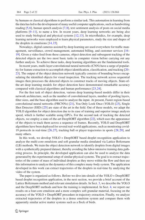
Fig. 1 a A triple emulsion with φ � 0.9 and Nd = 49 initialized within the inlet chamber. b Translocationdynamics of a dense emulsionφ = 0.9, Nd = 49 andhs/D � 0.45. Once the emulsion crosses the constriction,the resulting shape observed in the outlet chamber crucially depends on the area fraction φ

2 Lattice Boltzmann method and simulations

We employed two variants of the Lattice Boltzmann approach for the multicomponent flowssimulations, namely the color-gradient approach with near-contact interactions and the freeenergy model for multicomponent fluids. In Appendices A and B, we briefly outline the twomodels, while in the following sections, we report the simulation details for the two physicalsystems under consideration.

2.1 Simulation details for translocation of a soft granular material within narrow channels

This system is studied using the color gradient LB. The simulation setup consists of a two-dimensional microfluidic channel made of an inlet reservoir followed by a thinner channelconnected to a further downstream reservoir. The height of the chambers is h = 600 latticeunits and the one of the constriction is hs = 120 lattice units while its length is ls = 240lattice units. We impose a bounce-back rule for the distribution functions at the walls, whileat the outlet, we employ absorbing (zero gradient) [30].

The soft granular material is formed by droplets (component A, white region in Fig. 1)immersed within an inter-droplet continuous phase (component B, blue lines) surrounded byan external bulk phase (component C, black region outside the emulsion). Its structure closelyresembles that of a high internal phase double emulsion with multi-core morphology [31,32].In Fig. 1a we show a snapshot of the domain with the relevant dimension of the geometricalsetup and in Fig. 1b a translocation sequence of the soft material made of Nd = 49 internaldroplets occupying an area fraction φ � 0.9.

123

864 Page 4 of 22 Eur. Phys. J. Plus (2021) 136:864

In our numerical experiment, a uniform velocity profile of speedUin = 2×10−3 (in simu-lation units) is imposed at the inlet, which pushes the emulsion within the narrow constriction.Finally, the value of the velocity ensures that Capillary and Reynolds numbers remain wellwithin the typical range of microfluidic experiments (Ca ∼ O(10−3) and Re ∼ O(1)).

2.2 Simulation details for a flow of a multi-core emulsions within a microchannel.

Here we report the numerical details of the multi-core emulsion simulated using the free-energy LB. The droplet is set between two flat walls placed at distance Ly , where no-slipconditions hold for the velocity field v and neutral wetting for the fluid density ψ . The formermeans that the velocity is zero at the boundaries, while the latter that no mass flux crossesthe walls where droplet interfaces are perpendicular.

In Fig. 2 we show two examples of multi-core emulsions whose design is inspired byexperimental realizations. They are made of monodisperse immiscible droplets arrangedin a symmetric configuration. In Fig. 2a, three cores (white) of diameter Di = 30 latticesites are accommodated within a larger drop (black) of diameter DO = 100 lattice sites,in turn, surrounded by a further fluid (white). An analogous setup is used for the four-coreemulsion (see Fig. 2b). Starting from these configurations, the emulsions are then driven out ofequilibrium by applying a symmetric shear flow, where the top wall moves rightwards (alongthe positive x axis) at constant speed vw and the bottom wall in the opposite direction at speed−vw . This sets a shear rate of γ = 2Ly/vw . In previous works [33,34], it has been shownthat, once the shear is turned on, the external shell elongates and aligns along the directionimposed by the flow, while the internal cores acquire a periodic rotational motion triggeredby a fluid vortex formed within the emulsion. These dynamics persist over long periods oftime provided that the shear is on. In Fig. 2c, d we show two instantaneous configurations of athree and a four-core emulsion at late times, where γ � 10−4 with vw = 0.01 and Ly = 170in simulation units.

This system approximately corresponds to a real multi-core emulsion with a shell ofdiameter � 100μm and cores of diameter � 30μm, having a surface tension ranging between1 − 10mN/m, a viscosity � 10−1 Pa·s and a shear rates varying between 0.1 − 1/s. Like inthe previous method, Capillary and Reynolds numbers here range between 0.1 and 1 as well,as in typical microfluidic experiments.

The output of the simulations of the physical systems described above are saved as videofiles and later given as input to the deep learning-based application for automatic extractionof the trajectories of the moving droplets. In the supplementary material [35], see video1.avifile for the simulation output of translocation of triple emulsions within narrow channels andvideo2.avi for a flow of multi-core emulsions within a microchannel.

3 Technique

In this work, we develop an application to extract trajectories of individual droplets simulatedvia LB methods by adapting two different algorithms, one for object detection and anotherone for object tracking. The first task consists of training an artificial neural network toanalyze digital images and locate the objects of interest, which in this case are the droplets.Later, the second task is to track the located objects across multiple sequential frames toinfer their trajectories. Figure 3 shows the typical steps involved to accomplish the objectrecognition task [36]. In the following section, we briefly describe the algorithm employedfor the object recognition.

123

Eur. Phys. J. Plus (2021) 136:864 Page 5 of 22 864

(a) (b)

(c) (d)

x

y

Fig. 2 a, b Initial configurations of a three and a four-core monodisperse emulsion. The diameter of the coresis Di = 30 lattice sites while that of the shell is DO = 100 lattice sites. c, d Examples of instantaneousconfigurations of a the multi-core emulsions subject to a symmetric shear flow. The shear rate is γ � 10−4

in simulation units. In both cases internal cores rotate periodically clockwise, following an almost ellipticalpath triggered by the fluid vortex confined within the shell. For more details see Ref.[33,34]. Here Ca � 0.2and Re � 1.2

Fig. 3 Typical steps in developing the deep learning-based application for object detection. In the trainingphase, difference between prediction and truth is used to improve the accuracy of the network by updating theparameters of the network. At the inference stage, a real world data, in our case from LB simulation, is fed tothe network to obtain the bounding boxes around the droplets

123

864 Page 6 of 22 Eur. Phys. J. Plus (2021) 136:864

Fig. 4 High level sketch of the YOLO network structure

3.1 You only look once (YOLO)

You Only Look Once (YOLO) is a state-of-the-art algorithm that employs a single multi-layer network for object identification and classification. The YOLO algorithm has shownremarkable accuracy with high processing speed in identifying and classifying objects fromthe COCO dataset, which consists of 80 types (classes) of everyday objects [23].

The building structure of the YOLO network consists of two main components, a featureextractor and a detector. When an image is given as an input to the YOLO network, theextractor (also called backbone) produces feature representations at different scales (seeFig. 4). Such representations are then passed to the detector that outputs the bounding boxesalong with the confidence score and the classes of the detected objects. In this work, we usethe YOLO algorithm to identify droplets in the digital images produced by LB simulationsof two physical systems. We employ the YOLO-v3 network, which uses the Darknet-53network as a backbone. The Darknet-53 is a deep network consisting of 53 layers, whichhas shown significant improvement in object detection over its predecessors YOLO-v2 andYOLO-v1, which employ backbone with fewer layers [24].

The YOLO algorithm achieves high speed of image analysis due to its operating principle,namely by treating object detection as a regression instead of a classification task in deter-mining class probabilities to the bounding boxes. The operating procedure of the YOLOv3algorithm is sketched in Fig. 5. All objects in the given images are located and classifiedsimultaneously. To achieve that, the YOLO algorithm divides the input image into S × Sgrid cells. Each grid cell is responsible for detecting an object if the object’s center is withinthe cell domain. Each grid cell predicts B bounding boxes with their confidence score forthe object and C conditional class probabilities for the given object belonging to a specificclass. This information is then combined to produce the final output as a single bounding boxaround the detected object along with the class of that object. The final output is then passedto the DeepSORT algorithm for tracking the droplets.

3.2 DeepSORT

DeepSORT is an algorithm that tracks detected objects between two successive frames [22].By analyzing sequential frames, DeepSORT can construct trajectories of individual objects.It uses the Hungarian algorithm to distinguish the objects detected in two consecutive framesand assigns individual objects their unique identity. Kalman filtering is then used to predictthe future position of the objects based on their current positions.

The YOLO and the DeepSORT algorithms together accomplish droplet recognition andtracking from the simulated systems. In the next section, we outline the training data acqui-sition process employed in this work and later describe the training process for the YOLOnetwork for droplet detection.

123

Eur. Phys. J. Plus (2021) 136:864 Page 7 of 22 864

Fig. 5 Operating principle of the YOLO algorithm. Initially, an input image is split into S × S grid. In thenext stage, multiple bounding boxes are predicted along with a class probability map (blue color highlightscells hosting an object belonging to the “droplet” class) to give final bounding boxes and classes of objects

3.3 Training data

Before training a network, acquiring training data is a crucial part of an object detectionnetwork. Training data consists of several images of the objects to be detected along withinformation about their location and dimensions. Practically, acquiring the training data is alabor-intensive task involving gathering the images and manually marking the positions anddimensions of the objects. For example, gathering thousands of images of street view camerasand marking the location of the cars to train a network to identify cars in a video feed. Inaddition, the prospect of manual marking of the objects makes the training data susceptibleto human errors.

We avoided the labor-intensive process by preparing a synthetic training data set. Inthis dataset, each image is a collage with few solid white circles, mimicking the dropletsplaced randomly on a dark uniform background. The solid white circles of different sizesand shapes are prepared with commonly used computer graphics software. A separate textfile is generated to note the positions and dimensions of the randomly placed droplets. APython script generates several thousand images and associated text files in a matter of fewseconds. The script is provided in the supplementary material [35]. We prepared several typesof training datasets, and the detailed description is given in Appendix C.

We wish to emphasize that the training data, prepared synthetically, was intended tomimic the snapshots of the LB simulation, and it is not generated by a physical processassociated with LB simulations. However, it is noteworthy that the synthetic data preparationmethod described above bypasses the labor-intensive data acquisition part and minimizeshuman errors, thus making the development process of the droplet tracking application muchquicker and more precise. This method can potentially be used in several other object detectionapplications. In the next section, we describe the YOLO network’s training process to identifythe droplets with the synthetic data.

123

864 Page 8 of 22 Eur. Phys. J. Plus (2021) 136:864

Fig. 6 Total loss and mean average precision (mAP) as the training progresses. a YOLO-tiny network, bYOLO network

3.4 Training

The training of the YOLO network is carried out through an iterative process. A subset oftraining data, called batch size, is passed through the network in each iteration, and thenthe network predicts the bounding boxes around the detected objects. A loss value is com-puted based on the difference between the output and the ground truth. The supplied labelinformation is taken as the ground truth. The network parameters (weights and biases of thenodes) are updated to minimize the total loss and improve the accuracy of the network. Forthe YOLOv3 algorithm, the loss value, also called total loss, is the weighted sum of threeseparate contributions, regression loss, confidence loss, and classification loss [23]. In thetraining process, the weights of these contributions to the total loss are the same as proposedin Ref. [23] to optimize the mean average precision and maintain the model stability.

At regular intervals, i.e., after a few iterations, the accuracy of the network is assessed bycomputing mean average precision (mAP) [37,38]. The mean average precision is a goodmeasure to know how well the trained network performs on a dataset that is different fromthe training dataset. Typically, a separate dataset, called validation dataset, is compiled tocompute the mean average precision.

We trained two YOLO networks to identify the droplets from the LB simulations. Weadapted the code for training the network from Ref. [39]. The first network, called YOLO-tiny, is a lighter version of the full YOLO network consisting of fewer convolutional layersthan the full YOLO network to trade training and inference speed for accuracy. For manypractical purposes, the lighter version (YOLO-tiny) does perform reasonably well.

For training the YOLO-tiny network, we consolidated a total of 10000 images, consistingof an equal number of two different types of synthetic images as shown in Fig. 14a,b. Theparameters set for the training are mentioned here [40]. The parameters of the network areupdated at the end of every batch. A separate dataset of 1000 images, called validation data,was prepared from the same type of images to calculate the mean average precision. Thetotal loss and mean average precision as the training progresses are shown in Fig. 6a. As thetraining progresses, the total loss decreases, and the mean average precision of the networkincreases, indicating that the network is gaining performance with the training, reaching atotal loss value very close to zero at the end of the training. The mean average precision valueis saturated to 0.985, indicating that the network is 98.5% accurate in detecting the dropletsin broad terms.

123

Eur. Phys. J. Plus (2021) 136:864 Page 9 of 22 864

The second network we trained is the full YOLO network, with Darknet-53 as a backbone.Ten thousand images similar to the image shown in Fig. 14c were used as the training data.Another 1000 images of the same type were reserved as the validation data, and the trainingparameters are listed in [41]. In this case as well, as the training progresses, the total lossdecreases and mean average precision augments (as seen in Fig. 6b) saturating to 0.99, i.e.the network is 99% accurate in detecting the droplets. The trained model in the form of abinary file containing the model’s parameters (called weights) is saved. The weight file willbe used later to analyze the data from LB simulations, and it is provided for both networks,the YOLO-tiny and the YOLO, as supplementary material [35].

By training the YOLO network, we accomplish the first task of droplet recognition from thedigital images, while the DeepSORT algorithm handles the second task of droplet tracking. Inthe next section, we analyze two LB simulations as case studies to test and use the developedapplication.

4 Results

After the model is trained with the desired accuracy in terms of mean average precision,it is ready to analyze the real-world data. From simulations or experiments, the real wordimages can be given as input to the trained network, and individual droplets’ trajectories canbe obtained. This process is also called inference.

We run inference on the data generated with two LB simulations to test our trained networkas described in Sect. 2. For inference, only the droplets (white color mass) were plotted on adark background. The output video was then fed to the YOLO + DeepSORT network to inferthe trajectories of individual droplets. We adapted code with Tensorflow implementation torun inference from Ref. [42].

4.1 Multi-core emulsions

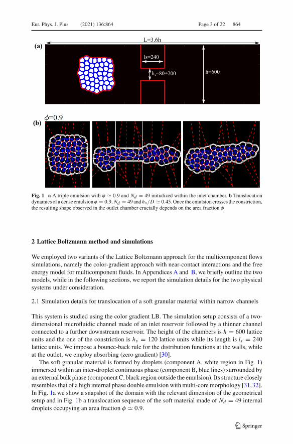
Figure 7 shows a visual depiction of the object recognition by the YOLO network andtracking of the located objects by the DeepSORT network in four sequential images from theLB simulations. The bounding boxes predicted by the YOLO network are shown in blue color,and the unique ID assigned by the DeepSORT algorithm is written above each bounding box(see video3.avi).

It is then straightforward to extract trajectories of the individual droplets across sequentialframes since we have dimensions of all the bounding boxes in all the frames with their uniqueID. The center of mass of the individual droplets is approximated as the geometric center ofits bounding box. Figure 8 shows the paths traced by the droplets.

4.2 Soft granular media

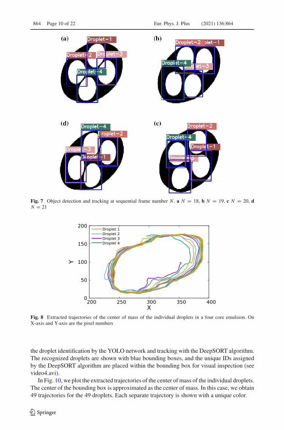
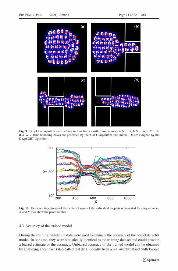
In the second case, we run inference on LB simulation of soft granular media. This time, weemployed the YOLO network to identify the droplets since the trained YOLO-tiny networkmakes many mistakes in droplet recognition. This is likely due to the increased complexityof the system, which presents a densely packed configuration of droplets moving through anarrow channel significantly deviating from its initial shape.

The YOLO network, however, can locate the droplets with almost perfect accuracy. Here,we note again that the training of the YOLO network was carried out with the training dataconsisting of randomly placed dense clusters of solid white circles. As before, Fig. 9 shows

123

864 Page 10 of 22 Eur. Phys. J. Plus (2021) 136:864

Fig. 7 Object detection and tracking at sequential frame number N . a N = 18, b N = 19, c N = 20, dN = 21

Fig. 8 Extracted trajectories of the center of mass of the individual droplets in a four core emulsion. OnX-axis and Y-axis are the pixel numbers

the droplet identification by the YOLO network and tracking with the DeepSORT algorithm.The recognized droplets are shown with blue bounding boxes, and the unique IDs assignedby the DeepSORT algorithm are placed within the bounding box for visual inspection (seevideo4.avi).

In Fig. 10, we plot the extracted trajectories of the center of mass of the individual droplets.The center of the bounding box is approximated as the center of mass. In this case, we obtain49 trajectories for the 49 droplets. Each separate trajectory is shown with a unique color.

123

Eur. Phys. J. Plus (2021) 136:864 Page 11 of 22 864

Fig. 9 Droplet recognition and tracking in four frames with frame number a N = 5, b N = 6, c N = 8,d N = 9. Blue bounding boxes are generated by the YOLO algorithm and unique IDs are assigned by theDeepSORT algorithm

Fig. 10 Extracted trajectories of the center of mass of the individual droplets represented by unique colors.X and Y axis show the pixel number

4.3 Accuracy of the trained model

During the training, validation data were used to estimate the accuracy of the object detectormodel. In our case, they were statistically identical to the training dataset and could providea biased estimate of the accuracy. Unbiased accuracy of the trained model can be obtainedby analyzing a test case (also called test data), ideally from a real-world dataset with known

123

864 Page 12 of 22 Eur. Phys. J. Plus (2021) 136:864

(a) (b)

(c) (d)

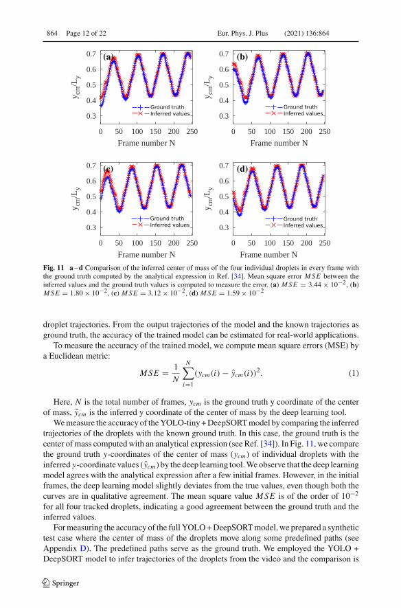
Fig. 11 a–d Comparison of the inferred center of mass of the four individual droplets in every frame withthe ground truth computed by the analytical expression in Ref. [34]. Mean square error MSE between theinferred values and the ground truth values is computed to measure the error. (a) MSE = 3.44 × 10−2, (b)MSE = 1.80 × 10−2, (c) MSE = 3.12 × 10−2, (d) MSE = 1.59 × 10−2

droplet trajectories. From the output trajectories of the model and the known trajectories asground truth, the accuracy of the trained model can be estimated for real-world applications.

To measure the accuracy of the trained model, we compute mean square errors (MSE) bya Euclidean metric:

MSE = 1

N

N∑

i=1

(ycm(i) − ycm(i))2. (1)

Here, N is the total number of frames, ycm is the ground truth y coordinate of the centerof mass, ycm is the inferred y coordinate of the center of mass by the deep learning tool.

We measure the accuracy of the YOLO-tiny + DeepSORT model by comparing the inferredtrajectories of the droplets with the known ground truth. In this case, the ground truth is thecenter of mass computed with an analytical expression (see Ref. [34]). In Fig. 11, we comparethe ground truth y-coordinates of the center of mass (ycm) of individual droplets with theinferred y-coordinate values (ycm) by the deep learning tool. We observe that the deep learningmodel agrees with the analytical expression after a few initial frames. However, in the initialframes, the deep learning model slightly deviates from the true values, even though both thecurves are in qualitative agreement. The mean square value MSE is of the order of 10−2

for all four tracked droplets, indicating a good agreement between the ground truth and theinferred values.

For measuring the accuracy of the full YOLO + DeepSORT model, we prepared a synthetictest case where the center of mass of the droplets move along some predefined paths (seeAppendix D). The predefined paths serve as the ground truth. We employed the YOLO +DeepSORT model to infer trajectories of the droplets from the video and the comparison is

123

Eur. Phys. J. Plus (2021) 136:864 Page 13 of 22 864

(a) (b)

(c) (d)

Fig. 12 Measuring accuracy of the YOLO + DeepSORT model. a–d Inferred path of four different dropletscompared with their predefined paths. Mean square error MSE between the inferred values and the groundtruth values is computed to measure the error. (a) MSE = 1.41 × 10−4, (b) MSE = 1.52 × 10−4, (c)MSE = 1.55 × 10−4, (d) MSE = 1.45 × 10−4

shown in Fig. 12. Four droplets were tracked and the inferred path is compared with the knownpredefined trajectories of these droplets. Both the trajectories are in excellent agreement andwe see no deviation in the inferred and true trajectories in any phase of the tracking. TheYOLO + DeepSORT model is highly accurate with MSE of the order of 10−4. The low valuesof mean square errors once again point to the high accuracy of the trained model.

We emphasize that we measure the accuracy of the developed application, including theobject recognition and the object tracking process. The error values are indicative of the totalexpected error in extracted trajectories from the real-world data. Apart from the model’saccuracy, the model’s analysis speed is an important factor to consider while developing anapplication for practical use. In the next section, we report the inference speed, i.e., the rate ofimage analysis by the developed application on different computer hardware configurations.

4.4 Inference speed

We test the inference speed of the object detection and tracking model on a typical notebookcomputer and a commonly used GPU machine. For inference, we used Tensorflow imple-mentation [42]. The inference speed, analyzed frame per second (FPS), for the YOLO-tinyand the YOLO network are tabulated in Table 1.

These data clearly show that there is room for improvement and optimization of theinference speed for both YOLO and DeepSORT, for instance, by coding them in other pro-gramming languages, such as C++. This is an interesting topic for future work.

Having accurate trajectories of moving objects is the first step to study the system. In thenext section, we present an analysis of the inferred trajectories to test a hypothesis.

123

864 Page 14 of 22 Eur. Phys. J. Plus (2021) 136:864

Table 1 Average inference speed in frames per second (fps) on two hardware configurations

Network/Machine Inference speed

CPU (i3-2328M) GPU (RTX 2060 Super)

YOLO-tiny + DeepSORT 2.44 fps 35 fps

YOLO + DeepSORT 0.25 fps 12 fps

Fig. 13 a Neighborhood of one of the randomly chosen droplet. The neighborhood of a droplet is a circlewith R = 30 pixels. b Scatter plot of the direction of individual droplets θi with the average moving directionof droplets θS in the neighbourhood of the droplet i . Values on the axes are in radians. The thick red line is aguideline to identify instances when the moving direction of droplets and their neighbors are identical

4.5 Flocks of droplets?

At first sight, the droplets seem to move like the agents in active matter systems, suchas birds in a flock. Several statistical physics models have been proposed to explain theflocking behavior in animal groups [43–45], and experimental studies involving observationof moving animal groups inferred the interaction rules between the agents [46,47]. Oneprominent feature common in most of these models is that the agents (birds) move along theaverage direction of their neighbors.

Given the superficial similarity between a flock and the soft granular media system studiedhere, we perform a quick analysis to test a hypothesis that the droplets behave like agentsin an active matter system. To this end, we calculate the average moving direction θS of theneighbors of each individual droplet. The neighbors of droplet i are defined as droplets withina circle of radius R, fixed on the center of the droplet i . We set the size of the neighborhoodin such a way that few neighboring droplets are included (see Fig. 13a). Figure 13b showsa scatter plot between individual droplet’s moving direction θi and the average direction oftheir neighbors θS for the entire duration of the simulation. The moving direction is measuredas angle θ made by the velocity vector with the x-axis in a fixed frame of reference. Thus,the range of θ is from −π to +π . Each different color in this plot shows a separate identityof the individual droplets. The red line is a guideline for the eyes to show the situation whenthe individual droplet’s moving direction is identical to that of its neighbors.

In Fig. 13, around 47% of all the total points are in the band when |θi − θS | < 0.12. i.e.,when the angle between the droplet’s motion and its neighbors is less than 7 degrees. Thissuggests that the moving direction of individual droplet deviates (by more than 7 degrees)from the average direction of their neighbors 53% of the time.

123

Eur. Phys. J. Plus (2021) 136:864 Page 15 of 22 864

We conclude that individual droplets frequently deviate from the average direction of theirneighbors than the individual birds do in a polarized flock. This is plausible since, besidessome similarities, there are also several points of departure between the two systems. First, insoft granular media systems, the fluid flow carries the droplets along the flow direction, like asystematic wind and second, the wall boundaries impose a stringent constraint on the motionof the droplets. None of the two aspects above are generally considered in the modeling ofactive matter systems.

In this analysis, we compared only the polarization between the system of droplets andthe ordered flock. Numerous other observations characterize a flock [48], and a detailedcomparison is required to quantify the similarities between these two systems. Nevertheless,this raises an interesting question on how to generalize the flock equations to come up witha set of effective equations of the droplets in complex many-body flows such as the oneexplored here. We plan to address this question in future work.

5 Conclusions

We adapted and combined deep learning-based object recognition algorithm YOLO andobject tracking algorithm DeepSORT to analyze data generated by fluid simulations of twosoft flowing systems, multicore emulsions, and soft granular media. In particular, the trajec-tories of the individual droplets moving within a microchannel flow were extracted from thedigital images of the system.

We determine the accuracy of the complete application by comparing the inferred tra-jectories with the ground truth trajectories computed by independent methods. Although weused LB simulation data as a case study; the developed application can also be applied datagenerated by two-dimensional experimental setups.

With the use of commonly available GPUs, the YOLO + DeepSORT based applicationcan analyze the images at a remarkable rate, above the image capture rate of typical cameras,thus offering a practical, low-cost application capable of analyzing real-time data as it isacquired.

From the technical point of view, we showed that the synthetically prepared datasets couldbe used to train the object detection network with almost perfect accuracy, thus avoiding labor-intensive, time-consuming training data acquisition for object recognition network training.

We combined two state-of-the-art algorithms to identify and track the droplets and testedthe model on two physical systems. It would be interesting to see how the application works forother dense emulsion systems. Nevertheless, YOLO and DeepSORT have shown remarkableperformance in object recognition and tracking in more complex environments. We hopeand expect that further developments of the work presented here may pave the way to theautomatic detection and tracking of moving agents in complex flows of scientific, engineering,and biological interest.

Acknowledgements M. D., F. B., A. M., M. L., A. T. and S. S. acknowledge funding from the EuropeanResearch Council under the European Union’s Horizon 2020 Framework Programme (No. FP/2014-2020)ERC Grant Agreement No.739964 (COPMAT)

Funding Open access funding provided by Istituto Italiano di Tecnologia within the CRUI-CARE Agreement.

Data Availability Statement This manuscript has associated data in a data repository. [Authors comment:All data generated or analysed during this study are included in this published article.]

123

864 Page 16 of 22 Eur. Phys. J. Plus (2021) 136:864

Open Access This article is licensed under a Creative Commons Attribution 4.0 International License, whichpermits use, sharing, adaptation, distribution and reproduction in any medium or format, as long as you giveappropriate credit to the original author(s) and the source, provide a link to the Creative Commons licence,and indicate if changes were made. The images or other third party material in this article are included in thearticle’s Creative Commons licence, unless indicated otherwise in a credit line to the material. If material isnot included in the article’s Creative Commons licence and your intended use is not permitted by statutoryregulation or exceeds the permitted use, you will need to obtain permission directly from the copyright holder.To view a copy of this licence, visit http://creativecommons.org/licenses/by/4.0/.

A Color-gradient approach with near contact interactions

Here we describe the LB approach used to simulate the translocation through a constrictionof a high internal phase double emulsion. We employ a color-gradient [49–54] regularizedLB method [55–57], which is built starting from two sets of probability distribution functionscapturing the dynamics of the immiscible fluid components. Each set evolves via a sequenceof streaming and collision steps [30,58–60]

f ki (x + ciΔt, t + Δt) = f ki (x, t) + Ωki ( f ki (x, t)) + Frep

i , (2)

where f ki (x, t) is the i th discrete probability distribution function for the kth component,giving the probability of finding a fluid particle at position x, time t and with discrete velocityci . The index k is such that k = 1, 2, while i belongs to the range 0 ≤ i ≤ Nset , where Nset

is the dimension of the set of discrete probability distribution functions and is equal to 8 forthe two-dimensional nine speeds lattice (D2Q9) employed in this paper. The time step Δt isexpressed in lattice units [30] and set to 1, a usual choice in the LB methods [58]. Finally,Frepi is a force aimed at upscaling the repulsive near-contact forces acting on scales much

smaller than the resolved ones [61,62].As stated above, the multicomponent approach employed in this work is based on a variant

of the color-gradient LB model. Following the standard formalism, the collision operator canbe split into three parts

Ωki = (Ωk

i )(3)[(Ωki )(1) + (Ωk

i )(2)]. (3)

The first term (Ωki )(1) is the usual single relaxation time Bhatnagar–Gross–Krook collisional

operator [58] while the second part (Ωki )(2) is the perturbation step, which accounts for the

interfacial tension, and reads as

(Ωki )(2) = Ak

2|∇Θ|

(wi

(ci · ∇Θ

|∇Θ|)2

− Bi

), (4)

where Ak (k = 1, 2) and Bi (i = 0, Nset ) are suitable constants defined in [61]. In Eq. (4),Θ is a scalar phase field, defined as

Θ = ρ1 − ρ2

ρ1 + ρ2(5)

assuming the value 1 in the fluid component with density ρ1 and the value −1 in the fluidcomponent with density ρ2. It is worth observing that the constants A1, A2 are related to thesurface tension σ by

σ = 2

9τ(A1 + A2). (6)

The third term (Ωki )(3) is the recolouring operator, as described in [63], which aims at mini-

mizing the mutual diffusion between the fluid components, thus favouring their separation.

123

Eur. Phys. J. Plus (2021) 136:864 Page 17 of 22 864

Finally, the last term at the right hand side of Eq. (2) codes for the short-range, repulsiveforce at the interface between the two fluid components, aimed at frustrating the coalescencebetween interacting, neighboring droplets.

B Free energy LB models for interacting multicomponent fluids

In this subsection we shortly outline the multicomponent field model for immiscible fluidmixtures employed to simulate the physics of three and four-core emulsions. Further detailscan be found in [33,34,64–66].

In this approach, a set of scalar phase-fields ψi (r, t), i = 1, ...., M (where M is thenumber of cores) is used to model the droplet density (positive within each drop and zerooutside), while the average fluid velocity of both drops and solvent is described by a vectorfield v(r, t).

The dynamics of the fields ψi (r, t) is governed by a set of convection-diffusion equations

∂tψi + v · ∇ψi = D∇2μi , (7)

where D is the mobility, μi = δFδψi

is the chemical potential and F = ∫V f dV is the total

free energy describing the equilibrium properties of the fluid suspension. The free energydensity f is given by [67,68]

f = a

4

M∑

i

ψ2i (ψi − ψ0)

2 + k

2

M∑

i

(∇ψi )2 + ε

∑

i, j,i< j

ψiψ j , (8)

where the first term is the double-well potential ensuring the existence of two coexistingminima, ψi = ψ0 inside the i th droplet and ψi = 0 outside, and the second term stabilizesthe droplet interface. The parameters a and k are two positive constants related to the surfacetension σ = √

8ak/9 and the width of interface ξ = 2√

2k/a [30,69]. Finally, the last termin Eq. (8) is a soft-core repulsion contribution which penalizes the overlap of droplets, andwhose strength is tuned by the positive constant ε.

The fluid velocity v obeys the Navier-Stokes equation, which in the incompressible limitreads

ρ

(∂

∂t+ v · ∇

)v = −∇ p + η∇2v −

∑

i

ψi∇μi . (9)

Here ρ is the fluid density, p is the isotropic pressure and η is the dynamic viscosity. A typicalset of values of thermodynamic parameters used in simulations is the following: a = 0.07,k = 0.1, D = 0.1, η = 1.67, ε = 0.05, Δx = 1 (lattice step), Δt = 1 (time step).

Equations (7) are solved using a finite difference scheme while Eq. (9) is integrated bymeans of a standard lattice Boltzmann method. The latter shares many features with the LBmodel described in the previous section. Indeed, it is built from a set of distribution functionswhose evolution is governed by a discrete Boltzmann equation akin to Eq. (2) and defined on aD2Q9 lattice. In both methods it can be shown that, once conservation of mass and momentumare fulfilled, the Navier-Stokes equation can be obtained by performing a Chapman-Enskogexpansion of the distribution functions [58,70]. However, unlike the previous algorithm, inthis approach the thermodynamics is encoded in a free-energy employed to calculate theforces (chemical potential and pressure tensor) controlling the relaxation dynamics of themixture. In addition, this model allows for an immediate tracking of position and speed ofthe droplets by computing the coordinates of the center of mass.

123

864 Page 18 of 22 Eur. Phys. J. Plus (2021) 136:864

C Training data

Training data is used to train the YOLO network to locate the droplets in given input images.Now we describe the training data acquisition employed in this work. Training data for theYOLO network must consist of several images of the objects of interest and their positionsin the images. Training data is passed through the network, and the network parameters areupdated with every pass to increase the detection accuracy. In a typical exercise to train anetwork, training data is compiled by acquiring images taken by digital cameras in the realworld. Objects in those images are manually identified and marked with bounding boxesencapsulating each object. A separate label file containing the class of the object, positions(x,y coordinates), and dimensions (width and height) of the bounding boxes is prepared.

We avoided the labor-intensive part of image acquisition and manual labeling by preparinga synthetic training dataset. The training dataset must contain several images that bear somevisual features of the expected outcome of the LB simulations, as shown in Figs. 1 and 2.In our case, the outcome of the LB simulations are the images with the area occupied by thedroplets shown by white color on a high contrast dark background. We prepared our trainingdataset by randomly placing solid white circles on a dark uniform background. The solidwhite circles were intended to resemble the droplets, and the high contrast background isintended for easy identification of the droplets from the background.

In the case of LB simulation of multi-core emulsions, the outcome consists of few ellipticalshape droplets enclosed in a dark bag on a uniform white background. We incorporate thesefeatures in the training data set by preparing 10000 images each of two types of images. Thefirst type of images (see a representative Fig. 14a) are prepared by placing the white solidcircles and ellipses of randomly chosen semi-minor and semi-major axis on the backgroundof size 1200 × 600 to teach the network to identify droplets of various sizes. In the secondtype of images (see Fig. 14b), two solid circles as droplets are placed randomly within a solidblack circle. The position of the solid black circle is chosen randomly in the uniform whitebackground.

Fig. 14 a Randomly placed droplets on a black uniform background of size 1200 × 600. b Two dropletsare randomly placed in a black envelope. The placement of the envelope is random within the white uniformbackground of size 1200 × 600 pixels. c Few random size clusters of droplets were placed randomly in auniform background of size 1200 × 600. d Label information associated with each of the bounding boxes

123

Eur. Phys. J. Plus (2021) 136:864 Page 19 of 22 864

In the case of LB simulations of soft granular media, the most apparent feature is thedense droplets cluster. In this case, few clusters with the random number of solid whitecircles are placed in a uniform solid black background to compile training data. The trainingdata consisted of 10000 such images (see Fig. 14c as an example).

The label information for every image is shown in Fig. 14d. Each bounding box enclosesa single white droplet. In associated text files, the dimensions of the bounding boxes (x and ycoordinates, width and height, and the class of object it encapsulates) are noted down. Imagesand the training data together form a training dataset for the YOLO network.

D Synthetic test case

To measure the accuracy of the developed YOLO + DeepSORT application, we prepared atest video. In this video, the center of mass of each droplet move along predefined trajectories(see video5.avi). The following equation gives the trajectory of individual droplets;

xi (t + 1) = xi (t) + A,

yi (t + 1) = yi (t) + B sin(kxi (t)).(10)

Here, xi (t) and yi (t) are the coordinates of the i th droplet at time t. A, B and k are thesuitable constants set as A = 5, B = 5 and k = 5.

In practice, we prepared several images and in each image we pasted 12 droplets at thelocation given by Eq. (10). Each droplet was placed with a random initial location, i.e. atpixel location given as (yi (t = 0),xi (t = 0)). These images were then sequentially stackedto prepare a video of continuously moving droplets on predefined paths. In Fig. 15 we showone instance of the droplet identification and tracking process. See video6.avi for the outputof the developed application.

Fig. 15 Snapshot of the output from YOLO + DeepSORT network to track droplets moving on predefinedpaths. Blue boxes are predictions by the YOLO network, and the DeepSORT network assigned unique ids

123

864 Page 20 of 22 Eur. Phys. J. Plus (2021) 136:864

References

1. S. Succi, P.V. Coveney, Big data: the end of the scientific method? Philosoph. Transac. Royal Soc. A:Math. Phys. Eng. Sci. 377(2142), 20180145 (2019)

2. C. Rudin, K.L. Wagstaff, Machine learning for science and society. Mach. Learn. 95, 1–9 (2014)3. M.G. Schultz, C. Betancourt, B. Gong, F. Kleinert, M. Langguth, L.H. Leufen, A. Mozaffari, S. Stadtler,

Can deep learning beat numerical weather prediction? Philosoph. Transac. Royal Soc. A Mathe. Phys.Eng. Sci. 379(2194), 20200097 (2021)

4. Y. LeCun, Y. Bengio, G. Hinton, Deep learning. Nature 521, 436–444 (2015)5. Darmatasia, M. I. Fanany, Handwriting recognition on form document using convolutional neural net-

work and support vector machines (cnn-svm), 2017 5th International Conference on Information andCommunication Technology (ICoIC7), pp. 1–6, (2017)

6. S. Ahlawat, A. Choudhary, A. Nayyar, S. Singh, B. Yoon, Improved handwritten digit recognition usingconvolutional neural networks (cnn), Sensors, 20(12), (2020)

7. N. H. Tandel, H. B. Prajapati, V. K. Dabhi, Voice recognition and voice comparison using machine learningtechniques: A survey, 2020 6th International Conference on Advanced Computing and CommunicationSystems (ICACCS), pp. 459–465, (2020)

8. K. Han, D. Yu, I. Tashev, Speech emotion recognition using deep neural network and extreme learningmachine, in Interspeech 2014, (2014)

9. A. Severyn and A. Moschitti, Unitn: Training deep convolutional neural network for twitter sentimentclassification, Proceedings of the 9th International Workshop on Semantic Evaluation (SemEval 2015),pp. 464–469, (2015)

10. A. M. Ramadhani, H. S. Goo, Twitter sentiment analysis using deep learning methods, 2017 7th Interna-tional Annual Engineering Seminar (InAES), pp. 1–4, (2017)

11. L. Zhang, S. Wang, B. Liu, Deep learning for sentiment analysis: a survey. WIREs Data Min. Knowl.Discovery 8(4), e1253 (2018)

12. G. Carleo, I. Cirac, K. Cranmer, L. Daudet, M. Schuld, N. Tishby, L. Vogt-Maranto, L. Zdeborová,Machine learning and the physical sciences. Rev. Mod. Phys. 91, 045002 (2019)

13. A.W. Senior, R. Evans, J. Jumper, J. Kirkpatrick, L. Sifre, T. Green, C. Qin, A. Žídek, A.W.R. Nelson,A. Bridgland, H. Penedones, S. Petersen, K. Simonyan, S. Crossan, P. Kohli, D.T. Jones, D. Silver, K.Kavukcuoglu, D. Hassabis, Improved protein structure prediction using potentials from deep learning.Nature 577, 706–710 (2020)

14. J.W. Khor, N. Jean, E.S. Luxenberg, S. Ermon, S.K.Y. Tang, Using machine learning to discover shapedescriptors for predicting emulsion stability in a microfluidic channel. Soft Matt. 15, 1361–1372 (2019)

15. Y. Mahdi, K. Daoud, Microdroplet size prediction in microfluidic systems via artificial neural networkmodeling for water-in-oil emulsion formulation. J. Dispersion Sci. Technol. 38(10), 1501–1508 (2017)

16. T. Osman, S. S. Psyche, J. M. Shafi Ferdous, H. U. Zaman, Intelligent traffic management system forcross section of roads using computer vision, 2017 IEEE 7th Annual Computing and CommunicationWorkshop and Conference (CCWC), pp. 1–7, (2017)

17. G. T. S. Ho, Y. P. Tsang, C. H. Wu, W. H. Wong, K. L. Choy, A computer vision-based roadside occupationsurveillance system for intelligent transport in smart cities, Sensors, 19(8), (2019)

18. B. Yogameena, C. Nagananthini, Computer vision based crowd disaster avoidance system: a survey. IntJ Disaster Risk Reduction 22, 95–129 (2017)

19. N. Ragesh, B. Giridhar, D. Lingeshwaran, P. Siddharth, K. P. Peeyush, Deep learning based automatedbilling cart, 2019 International Conference on Communication and Signal Processing (ICCSP), pp. 0779–0782, (2019)

20. R. L. Galvez, A. A. Bandala, E. P. Dadios, R. R. P. Vicerra, J. M. Z. Maningo, Object detection usingconvolutional neural networks, TENCON 2018 - 2018 IEEE Region 10 Conference, pp. 2023–2027,(2018)

21. S. Ren, K. He, R. Girshick, J. Sun, Faster r-cnn: Towards real-time object detection with region proposalnetworks. IEEE Transac Pattern Analy Machine Intell 39(6), 1137–1149 (2017)

22. N. Wojke, A. Bewley, D. Paulus, “Simple online and realtime tracking with a deep association metric,”2017 IEEE International Conference on Image Processing (ICIP), pp. 3645–3649, (2017)

23. J. Redmon, S. Divvala, R. Girshick, A. Farhadi, “You only look once: Unified, real-time object detection,”2016 IEEE Conference on Computer Vision and Pattern Recognition (CVPR), pp. 779–788, (2016)

24. J. Redmon, A. Farhadi, “Yolov3: An incremental improvement,” ArXiv:1804.02767v1, (2018)25. W. Liu, D. Anguelov, D. Erhan, C. Szegedy, S. Reed, C.-Y. Fu, A.C. Berg, Ssd: Single shot multibox

detector. Comput. Vision - ECCV 2016, 21–37 (2016)26. N. S. Punn, S. K. Sonbhadra, S. Agarwal, G. Rai, Monitoring covid-19 social distancing with person detec-

tion and tracking via fine-tuned yolo v3 and deepsort techniques (2021). arXiv:2005.01385v4 [cs.CV]

123

Eur. Phys. J. Plus (2021) 136:864 Page 21 of 22 864

27. S. Khosravipour, E. Taghvaei, N. M. Charkari, Covid-19 personal protective equipment detection usingreal-time deep learning methods (2021). arXiv:2103.14878v1 [cs.CV]

28. T. Zhang, X. Zhang, Y. Yang, Z. Wang, G. Wang, Efficient golf ball detection and tracking based onconvolutional neural networks and kalman filter (2021). arXiv:2012.09393v2 [cs.CV]

29. K. Host, M. Ivašic-Kos, M. Pobar, “Tracking handball players with the deepsort algorithm,” in Proceedingsof the 9th International Conference on Pattern Recognition Applications and Methods - ICPRAM, pp. 593–599, INSTICC, SciTePress, (2020)

30. T. Krüger, H. Kusumaatmaja, A. Kuzmin, O. Shardt, G. Silva, E.M. Viggen, The lattice boltzmannmethod(Springer, Newyork, 2017)

31. M. Costantini, C. Colosi, J. Guzowski, A. Barbetta, J. Jaroszewicz, W. Swieszkowski, M. Dentini, P.Garstecki, Highly ordered and tunable polyhipes by using microfluidics. J. Mater. Chem. B 2, 2290–2300(2014)

32. A.S. Utada, E.L. Lorenceau, D.R. Link, P.D. Kaplan, H.A. Stone, D.A. Weitz, Monodisperse doubleemulsions generated from a microcapillary device. Science 308, 537–541 (2005)

33. A. Tiribocchi, A. Montessori, S. Aime, M. Milani, M. Lauricella, S. Succi, D.A. Weitz, Novel nonequi-librium steady states in multiple emulsions. Phys. Fluids 32, 017102 (2020)

34. A. Tiribocchi, A. Montessori, F. Bonaccorso, M. Lauricella, S. Succi, Concentrated phase emulsion withmulticore morphology under shear: a numerical study. Phys. Rev. Fluids 5, 113606 (2020)

35. https://cloud.degoo.com/share/R_EZJd7UptbslTVcuV6Rqg ,36. M. Durve, F. Bonaccorso, A. Montessori, M. Lauricella, A. Tiribocchi, S. Succi, A fast and effi-

cient deep learning procedure for tracking droplet motion in dense microfluidic emulsions (2021).arXiv:2103.01572v1 [cond-mat.soft]

37. M. Everingham, L. Van Gool, C.K.I. Williams, J. Winn, A. Zisserman, The pascal visual object classes(voc) challenge. Int. J. Comput. Vision 88, 303–338 (2010)

38. P. Henderson, V. Ferrari, “End-to-end training of object class detectors for mean average precision,”Computer Vision – ACCV 2016 Lecture Notes in Computer Science, 198–213, (2017)

39. J. Redmon, “Darknet: Open source neural networks in c.” http://pjreddie.com/darknet/, year, 2013–201640. Batches=10000, batch size=128, learning rate=0.00141. Batches=10000, batch size=64, learning rate=0.00142. https://github.com/theAIGuysCode/yolov3_deepsort43. T. Vicsek, A. Czirók, E. Ben-Jacob, I. Cohen, O. Shochet, Novel type of phase transition in a system of

self-driven particles. Phys. Rev. Lett. 75, 1226–1229 (1995)44. I.D. Couzin, J. Krause, R. James, G.D. Ruxton, N.R. Franks, Collective memory and spatial sorting in

animal groups. J. Theor. Biol. 218(1), 1–11 (2002)45. A. Cavagna, L. Del Castello, I. Giardina, T. Grigera, A. Jelic, S. Melillo, T. Mora, L. Parisi, E. Silvestri,

M. Viale, A.M. Walczak, Flocking and turning: a new model for self-organized collective motion. J. Stat.Phys. 158, 601–627 (2015)

46. J.E. Herbert-Read, A. Perna, R.P. Mann, T.M. Schaerf, D.J.T. Sumpter, A.J.W. Ward, Inferring the rulesof interaction of shoaling fish. Proc. Nat. Acad. Sci. 108(46), 18726–18731 (2011)

47. R. Lukeman, Y.-X. Li, L. Edelstein-Keshet, Inferring individual rules from collective behavior. Proc. Nat.Acad. Sci. 107(28), 12576–12580 (2010)

48. I. Giardina, Collective behavior in animal groups: theoretical models and empirical studies. HFSP Journal2, 205–219 (2008)

49. S. Leclaire, M. Reggio, J.-Y. Trépanier, Numerical evaluation of two recoloring operators for an immiscibletwo-phase flow lattice boltzmann model. Appl. Math. Model. 36(5), 2237–2252 (2012)

50. S. Leclaire, A. Parmigiani, O. Malaspinas, B. Chopard, J. Latt, Generalized three-dimensional latticeboltzmann color-gradient method for immiscible two-phase pore-scale imbibition and drainage in porousmedia. Phys. Rev. E 95, 033306 (2017)

51. A.K. Gunstensen, D.H. Rothman, S. Zaleski, G. Zanetti, Lattice boltzmann model of immiscible fluids.Phys. Rev. A 43, 4320 (1991)

52. A. Montessori, M. Lauricella, M. La Rocca, S. Succi, E. Stolovicki, R. Ziblat, D. Weitz, Regularizedlattice boltzmann multicomponent models for low capillary and reynolds microfluidics flows. Comput.Fluids 167, 33–39 (2018)

53. A. Montessori, M. Lauricella, S. Succi, E. Stolovicki, D. Weitz, Elucidating the mechanism of stepemulsification. Phys. Rev. F. 3, 072202 (2018)

54. D.H. Rothman, J.M. Keller, Immiscible cellular-automaton fluids. J. Stat. Phys. 52(3–4), 1119–1127(1988)

55. A. Montessori, P. Prestininzi, M. La Rocca, S. Succi, Lattice boltzmann approach for complex nonequi-librium flows. Phys. Rev. E 92(4), 043308 (2015)

123

864 Page 22 of 22 Eur. Phys. J. Plus (2021) 136:864

56. J. Latt, B. Chopard, Lattice boltzmann method with regularized pre-collision distribution functions. Math.Comput. Simul. 72(2–6), 165–168 (2006)

57. C. Coreixas, B. Chopard, J. Latt, Comprehensive comparison of collision models in the lattice boltzmannframework: theoretical investigations. Phys. Rev. E 100(3), 033305 (2019)

58. S. Succi, The Lattice Boltzmann equation: for complex states of flowing matter (Oxford University Press,London, 2018)

59. S. Succi, Lattice boltzmann 2038. EPL (Europhys. Lett.) 109(5), 50001 (2015)60. R. Benzi, S. Succi, M. Vergassola, The lattice boltzmann equation: theory and applications. Phys. Rep.

222(3), 145–197 (1992)61. A. Montessori, M. Lauricella, N. Tirelli, S. Succi, Mesoscale modelling of near-contact interactions for

complex flowing interfaces. J. Fluid Mech. 872, 327–347 (2019)62. A. Montessori, M. Lauricella, A. Tiribocchi, S. Succi, Modeling pattern formation in soft flowing crystals.

Phys. Rev. Fluids 4(7), 072201 (2019)63. M. Latva-Kokko, D.H. Rothman, Diffusion properties of gradient-based lattice boltzmann models of

immiscible fluids. Phys. Rev. E 71(5), 056702 (2005)64. M. Foglino, A.N. Morozov, O. Henrich, D. Marenduzzo, Flow of deformable droplets: discontinuous

shear thinning and velocity oscillations. Phys. Rev. Lett. 119, 208002 (2017)65. M. Foglino, A.N. Morozov, D. Marenduzzo, Rheology and microrheology of deformable droplet suspen-

sions. Soft Matter 14, 9361–9367 (2018)66. A. Tiribocchi, A. Montessori, M. Lauricella, F. Bonaccorso, S. Succi, S. Aime, M. Milani, D.A. Weitz,

The vortex-driven dynamics of droplets within droplets. Nat. Commun. 12, 82 (2021)67. S.R. De Groot, P. Mazur, Non-equilibrium thermodynamics (NY, Dover, New York, 1984)68. G. Lebon, D. Jou, J. Casas-Vazques,Understanding non-equilibrium thermodynamics: foundations, appli-

cations (Springer, Frontiers, 2008)69. J.S. Rowlinson, B. Widom, Molecular theory of capillarity (Clarendon Press, Oxford, 1982)70. L.N. Carenza, G. Gonnella, A. Lamura, G. Negro, A. Tiribocchi, Lattice boltzmann methods and active

fluids. Eur. Phys. J. E 42, 81 (2019)

123