
Tracking an air target in multistatic radar networksdiscovery.ucl.ac.uk/1347920/1/1347920.pdf · 3...
173
Tracking an air target in multistatic radar networks Alexandre Moriya Supervisor: Prof. H.D Griffiths A thesis submitted for the degree of Master of Philosophy of University College London Department of Electronic and Electrical Engineering University College London 26 th March 2012
Transcript of Tracking an air target in multistatic radar networksdiscovery.ucl.ac.uk/1347920/1/1347920.pdf · 3...

Tracking an air target in multistatic
radar networks
Alexandre Moriya
Supervisor:
Prof. H.D Griffiths
A thesis submitted for the degree of
Master of Philosophy
of
University College London
Department of Electronic and Electrical Engineering
University College London
26th
March 2012

2
I, Alexandre Moriya, confirm that the work presented in this thesis is my own and
has not been submitted in any form for another degree or diploma at any university
or other institute of tertiary education. Information derived from other sources has
been indicated in the thesis.
Alexandre Moriya
London, March 26th
, 2012.

3
Abstract
The first radars used in military scenarios to detect enemies were bistatic because the
technology that would allow a transmitter and a receiver to use the same antenna had
not been developed. Then, with the development of monostatic radars, there was
almost no interest in the bistatic radars subject. Nowadays, due to the fact that
monostatic radars alone have reached its limits in terms of performance and because
of the existence of new threats, the interest in bistatic and multistatic radars should
last longer. Bistatic and multistatic radars are particularly interesting in military
scenarios where it is important to be able to detect and track stealth targets and also
to be able to operate with minimized risks of being affected by jamming attacks.
This thesis investigates how much multistatic radars can surpass stand alone
monostatic radars when attempting to track a target. Simulations with different
geometries and different target trajectories are performed in order to assess the
tracking performance in each scenario. Tracking performance is assessed in terms of
estimated position, velocity and acceleration accuracies. Different geometries include
monostatic radar, netted monostatic radars, bistatic radars with target crossing and
not crossing the baseline, multistatic radars with only 1 TX and many RXs,
multistatic radars with many TXs and only 1 RX and multistatic radars with many
TXs and RXs. Simulations are performed using real radar characteristics in order to
assess whether it is possible to use navigation radars to track targets with low RCS.
The research herein presented shows that it is possible to achieve a good accuracy
configuring a geometry that is suitable for the requirements of a system. Also, from
the results of the simulations it is possible to understand why multistatic radars can
still work with acceptable accuracy if a TXs is lost/destroyed.

4
To my wife and parents…

5
Acknowledgements
I would like to thank my MPhil supervisor, Prof Hugh Griffiths, who has helped me
throughout the whole period of my research and has given important and smart
advice showing the best ways to achieve the objectives of this research and
supporting me whenever it was necessary.
I would like to acknowledge, as well, all the members of the Radar Group who with I
could attend interesting and important seminars and who also have contributed with
interesting questions during my seminars. I would also like to mention Prof Chris
Baker who has contributed with ideas in a very important moment of my research.
Likewise, I am grateful to have had the company of all my old and new friends that
have made my staying in UK an unforgettable experience.
Additionally, I would like to thank the Brazilian Navy who has sponsored this
research and an important and clever colleague, Commander Gelza de Moura
Barbosa, who have always supported me and helped me with important technical
information. From the Brazilian Navy, I am also grateful to Captain Fuad Gatti Kouri
and Captain Jorge Antonio Vasconcellos dos Santos and their staff at the Office of
the Brazilian Defence and Naval Attaché for all their support throughout my staying
in London.
To my parents, Yoshinobu e Mitie, my special thanks for all the support they have
been giving me since ever.
Finally, I would like to thank my wife, Etel, for all her love, support, advice and
effort so that I could be able to concentrate on my studies and research. Without her,
I would not be able to make it. I also thank our families for their unconditional
support from Brazil during our period in UK.

6
Contents
Abstract ....................................................................................................................... 3
Acknowledgements ..................................................................................................... 5
Contents ...................................................................................................................... 6
List of Figures ............................................................................................................. 8
List of Tables ............................................................................................................ 19
List of Symbols ......................................................................................................... 20
List of Acronyms ...................................................................................................... 23
1 Introduction ...................................................................................................... 25
1.1 Overview and Motivation ............................................................................ 25
1.1.1 The Problem of Tracking in a Radar Network ..................................... 29
1.2 Thesis Layout .............................................................................................. 34
2 The Proposed Approach .................................................................................. 36
2.1 Scope and Limitations ................................................................................. 37
3 Bistatic / Multistatic Radar ............................................................................. 39
3.1 Advantages .................................................................................................. 39
3.2 Disadvantages .............................................................................................. 40
3.3 Bistatic Radar Properties ............................................................................. 41
3.3.1 Bistatic Radar geometry ....................................................................... 41
3.3.2 Bistatic Doppler ................................................................................... 42
3.3.3 Bistatic Radar equation ........................................................................ 44
3.3.4 Bistatic Radar Cross Section (RCS) ..................................................... 46
3.4 Multistatic Radar ......................................................................................... 47
4 Tracking algorithms......................................................................................... 50
4.1 Simple Example........................................................................................... 50
4.2 Multistatic Tracking of a Target .................................................................. 52
5 Review of Previous Work ................................................................................ 54
5.1 Multistatic Radar ......................................................................................... 54
5.2 Multistatic Tracking .................................................................................... 58

7
5.3 Resource Management ................................................................................ 63
6 Simulations........................................................................................................ 65
6.1 Setting up the Environment ......................................................................... 65
6.2 Methodology................................................................................................ 66
6.3 Algorithms ................................................................................................... 80
6.3.1 Simulated Measurements ..................................................................... 80
6.3.2 Critically Damped g-h filter ................................................................. 82
6.3.3 Critically Damped g-h-k filter .............................................................. 82
6.3.4 Kalman Filter (KF) ............................................................................... 83
7 Results ............................................................................................................... 87
7.1 Measurements Results ................................................................................. 89
7.1.1 Monostatic ............................................................................................ 89
7.1.2 Bistatic.................................................................................................. 95
7.1.3 Multistatic (1 x N) .............................................................................. 101
7.1.4 Multistatic (M x 1) ............................................................................. 103
7.1.5 Measurements Summary Table .......................................................... 106
7.2 Tracking Results ........................................................................................ 109
7.2.1 Target 1 (straight line) ........................................................................ 111
7.2.2 Target 2 (spiral-like trajectory) .......................................................... 127
7.2.3 Tracking Summary Tables ................................................................. 148
7.3 Analysis ..................................................................................................... 151
7.4 Examples ................................................................................................... 155
8 Conclusions and Further Work .................................................................... 160
8.1 Summary.................................................................................................... 166
References ............................................................................................................... 167
Appendix A - Matlab Code.................................................................................... 173

8
List of Figures
Figure 1 - Monostatic Radar ...................................................................................... 26
Figure 2 - Bistatic Radar ............................................................................................ 26
Figure 3 - Multistatic Radar ....................................................................................... 27
Figure 4 - Bistatic Radar being jammed .................................................................... 28
Figure 5 - Pairs of bistatic radar using different kind of transmitters ........................ 28
Figure 6 - Monostatic Radars working either as a monostatic or bistatic radar ......... 29
Figure 7 - Centralized system .................................................................................... 30
Figure 8 - Decentralized system ................................................................................. 31
Figure 9 - Decentralized Data Fusion System using peer-to-peer communication
links ............................................................................................................................ 32
Figure 10 - Decentralized Data Fusion System using a central network facility ....... 33
Figure 11 - Hierarchical system ................................................................................. 33
Figure 12 - Bistatic Radar Geometry ......................................................................... 42
Figure 13 - Constant range ellipse (isorange contour) ............................................... 42
Figure 14 - Bistatic Radar Geometry and the variables involved in the Bistatic
Doppler (after [3]) ...................................................................................................... 43
Figure 15 - Radar Range Equation variables ............................................................. 46
Figure 16 – (after [18]) σB and θB as functions of frequency (or wavelength λ) ........ 47
Figure 17 - Tracking recursive algorithm .................................................................. 51
Figure 18 - Horizontal (red) and Vertical (blue) target trajectories with different
velocities and the radar located at (100,0) km. .......................................................... 67
Figure 19 – Measurement number vs x-axis errors (using 150 m and 30 mrad
standard deviations) ................................................................................................... 67
Figure 20 – Measurement number vs y-axis errors (using 150 m and 30 mrad
standard deviations) ................................................................................................... 67
Figure 21 - Measurement number vs x-axis errors (using 15 m and 30 mrad standard
deviations) .................................................................................................................. 68
Figure 22 - Measurement number vs y-axis errors (using 15 m and 30 mrad standard
deviations) .................................................................................................................. 68
Figure 23 - Measurement number vs x-axis errors (using 150 m and 3 mrad standard
deviations) .................................................................................................................. 68
Figure 24 - Measurement number vs y-axis errors (using 150 m and 3 mrad standard
deviations) .................................................................................................................. 68
Figure 25 – location of TX (black circle) and RX (black hexagram), true trajectory
(red line) and measurements (green line) ................................................................... 69
Figure 26 - Measurement number vs x-axis errors (using 150 m and 3 mrad standard
deviations) .................................................................................................................. 69
Figure 27 - Measurement number vs y-axis errors (using 150 m and 3 mrad standard
deviations) .................................................................................................................. 69
Figure 28 – Geometry with monostatic radar location (black circle) and target
trajectory .................................................................................................................... 71
Figure 29 - Measurement number vs x-axis errors (range and azimuth standard
deviations vary with distance to the radar) ................................................................ 71
Figure 30 - Measurement number vs y-axis errors (range and azimuth standard
deviations vary with distance to the radar) ................................................................ 71

9
Figure 31 – Geometry with radars location and target trajectory where black circle is
TX and black hexagram is RX ................................................................................... 71
Figure 32 - Measurement number vs x-axis errors (range and azimuth standard
deviations vary with distance to the radar) ................................................................ 72
Figure 33 - Measurement number vs y-axis errors (range and azimuth standard
deviations vary with distance to the radar) ................................................................ 72
Figure 34 – Geometry with radars location and target trajectory where black circle is
TX and black hexagram is RX ................................................................................... 73
Figure 35 – Bistatic angle along the target trajectory ................................................ 73
Figure 36 – x-position of the target vs x-axis errors................................................... 73
Figure 37 – x-position of the target vs y-axis errors................................................... 73
Figure 38 - x-position of the target vs x-axis errors after tracking filter .................... 74
Figure 39 - x-position of the target vs y-axis errors after tracking filter .................... 74
Figure 40 – x-position of the target vs x-axis (red) and y-axis (blue) estimated
velocity ....................................................................................................................... 74
Figure 41 - Geometry with radars location and target trajectory (red) where green and
cyan circles are monostatic radars. Green and cyan dots represent measurements
from each radar respectively ...................................................................................... 75
Figure 42 – Individual tracks (green and cyan dots) and fused track (black line) ..... 75
Figure 43 – Fused measurements (yellow) and track (black line) ............................. 75
Figure 44 - Geometry with radar location, target trajectory (red) and measurements
(green). The black circle is the monostatic radar ....................................................... 76
Figure 45 - Geometry with radars location where green, blue, red and magenta circles
are monostatic radars and the same colours of lines represent their respective
measurements ............................................................................................................. 76
Figure 46 – Track when only one radar (1.5 MW) is used ........................................ 76
Figure 47 – Fusion of tracks from each radar (4 radars of 375 kW) .......................... 76
Figure 48 - Track when only one radar (1.5 MW) is used ......................................... 77
Figure 49 - Fusion of tracks from each radar (4 radars of 375 kW) .......................... 77
Figure 50 - Geometry with radars location, target trajectory (red sinusoidal) and
measurements (green/blue) from each monostatic radar (green and blue circles) ..... 78
Figure 51 – Tracking (black line) using a g-h-k filter after doing fusion of
measurements (yellow) .............................................................................................. 78
Figure 52 - Tracking (black line) after doing fusion of measurements (yellow) using
a g-h filter ................................................................................................................... 78
Figure 53 – Estimated y-velocity (blue line) using a g-h filter. Black line is the true
velocity. Estimated x-velocity is illustrated by the red line (constant 200 m/s) ........ 79
Figure 54 – Estimated y-velocity (blue line) using a g-h-k filter. Black line is the true
velocity. Estimated x-velocity is illustrated by the red line (constant 200 m/s) ........ 79
Figure 55 – Estimated velocity (blue line) using a g-h-k filter. Black line is the true
velocity ....................................................................................................................... 79
Figure 56 – test for Equation (36), when Power is 25 kw, RCS 0.1 m2..................... 85
Figure 57 – test for Equation (37), when Power is 25 kw, RCS 0.1 m2..................... 85
Figure 58 – Location of TX/RX (monostatic radar with 25 kW), true trajectory (red
line) and measurements (green dots).......................................................................... 90
Figure 59 - x-position vs x-axis errors (1 radar 25 kW) ............................................. 90
Figure 60 - x-position vs y-axis errors (1 radar 25 kW) ............................................. 90
Figure 61 – x-position vs SNR (blue line) – 1 radar 25 kW ...................................... 90
Figure 62 – x-position vs [range stddev(blue) and azimuth stddev (green)] – 1 radar
25 kW ......................................................................................................................... 90

10
Figure 63 - x-position vs x-axis errors (1 radar 6.25 kW) .......................................... 91
Figure 64 - x-position vs y-axis errors (1 radar 6.25 kW) .......................................... 91
Figure 65 – x-position vs SNR (blue line) – 1 radar 6.25 kW ................................... 91
Figure 66 – x-position vs [range stddev(blue) and azimuth stddev (green)] – 1 radar
6.25 kW ...................................................................................................................... 91
Figure 67 – Location of TX/RX (monostatic radar with 25 kW), true trajectory (red
line) and measurements (green dots).......................................................................... 91
Figure 68 - x-position vs x-axis errors (1 radar 25 kW) ............................................. 92
Figure 69 - x-position vs y-axis errors (1 radar 25 kW) ............................................. 92
Figure 70 – x-position vs SNR (blue line) – 1 radar 25 kW ...................................... 92
Figure 71 – x-position vs [range stddev(blue) and azimuth stddev (green)] – 1 radar
25 kW ......................................................................................................................... 92
Figure 72 – Location of TX/RX (monostatic radar with 6.25 kW), true trajectory (red
line) and measurements (green dots).......................................................................... 93
Figure 73 - x-position vs x-axis errors (1 radar 6.25 kW) .......................................... 93
Figure 74 - x-position vs y-axis errors (1 radar 6.25 kW) .......................................... 93
Figure 75 – x-position vs SNR (blue line) – 1 radar 6.25 kW ................................... 93
Figure 76 – x-position vs [range stddev(blue) and azimuth stddev (green)] – 1 radar
6.25 kW ...................................................................................................................... 93
Figure 77 - Location of TX/RX (monostatic radar with 25 kW), true trajectory (red
line) and measurements (green dots).......................................................................... 94
Figure 78 - x-position vs x-axis errors (1 radar 25 kW) ............................................. 94
Figure 79 - x-position vs y-axis errors (1 radar 25 kW) ............................................. 94
Figure 80 – x-position vs SNR (blue line) – 1 radar 25 kW ...................................... 94
Figure 81 – x-position vs [range stddev(blue) and azimuth stddev (green)] – 1 radar
25 kW ......................................................................................................................... 94
Figure 82 – Location of TX/RX (monostatic radar with 25 kW), true trajectory (red
line) and measurements (green dots).......................................................................... 95
Figure 83 - x-position vs x-axis errors (1 radar 25 kW) ............................................. 95
Figure 84 - x-position vs y-axis errors (1 radar 25 kW) ............................................. 95
Figure 85 – x-position vs SNR (blue line) – 1 radar 25 kW ...................................... 95
Figure 86 – x-position vs [range stddev(blue) and azimuth stddev (green)] – 1 radar
25 kW ......................................................................................................................... 95
Figure 87 - Location of TX and RX (bistatic radar with TX 25 kW), true trajectory
(red line) and measurements (green dots) .................................................................. 96
Figure 88 - x-position vs x-axis errors (1 TX 25 kW) ................................................ 96
Figure 89 - x-position vs y-axis errors (1 TX 25 kW) ................................................ 96
Figure 90 – x-position vs [SNR (blue line) and bistatic angle (green line) – 1 TX 25
kW .............................................................................................................................. 96
Figure 91 – x-position vs [range stddev(blue) and azimuth stddev (green)] – 1 TX 25
kW .............................................................................................................................. 96
Figure 92 - Location of TX and RX (bistatic radar with TX 25 kW), true trajectory
(red line) and measurements (green dots) .................................................................. 97
Figure 93 - x-position vs x-axis errors (1 TX 25 kW) ................................................ 97
Figure 94 - x-position vs y-axis errors (1 TX 25 kW) ................................................ 97
Figure 95 – x-position vs [SNR (blue line) and bistatic angle (green line) – 1 TX 25
kW .............................................................................................................................. 97
Figure 96 – x-position vs [range stddev(blue) and azimuth stddev (green)] – 1 TX 25
kW .............................................................................................................................. 97

11
Figure 97 - Location of TX and RX (bistatic radar with TX 6.25 kW), true trajectory
(red line) and measurements (green dots) .................................................................. 98
Figure 98 - x-position vs x-axis errors (1 TX 6.25 kW) ............................................. 98
Figure 99 - x-position vs y-axis errors (1 TX 6.25 kW) ............................................. 98
Figure 100 – x-position vs [SNR (blue line) and bistatic angle (green line) – 1 TX
6.25 kW ...................................................................................................................... 98
Figure 101 – x-position vs [range stddev(blue) and azimuth stddev (green)] – 1 TX
6.25 kW ...................................................................................................................... 98
Figure 102 - Location of TX and RX (bistatic radar with TX 6.25 kW), true
trajectory (red line) and measurements (green dots) .................................................. 99
Figure 103 - x-position vs x-axis errors (1 TX 6.25 kW) ........................................... 99
Figure 104 - x-position vs y-axis errors (1 TX 6.25 kW) ........................................... 99
Figure 105 – x-position vs [SNR (blue line) and bistatic angle (green line) – 1 TX
6.25 kW ...................................................................................................................... 99
Figure 106 – x-position vs [range stddev(blue) and azimuth stddev (green)] – 1 TX
6.25 kW ...................................................................................................................... 99
Figure 107 - Location of TX and RX (bistatic radar with TX 25 kW), true trajectory
(red line) and measurements (green dots) ................................................................ 100
Figure 108 - x-position vs x-axis errors (1 TX 25 kW) ............................................ 100
Figure 109 - x-position vs y-axis errors (1 TX 25 kW) ............................................ 100
Figure 110 – x-position vs [SNR (blue line) and bistatic angle (green line) – 1 TX 25
kW ............................................................................................................................ 100
Figure 111 – x-position vs [range stddev(blue) and azimuth stddev (green)] – 1 TX
25 kW ....................................................................................................................... 100
Figure 112 - Location of TX and RX (bistatic radar with TX 25 kW), true trajectory
(red line) and measurements (green dots) ................................................................ 101
Figure 113 - x-position vs x-axis errors (1 TX 25 kW) ............................................ 101
Figure 114 - x-position vs y-axis errors (1 TX 25 kW) ............................................ 101
Figure 115 – x-position vs [SNR (blue line) and bistatic angle (green line) – 1 TX 25
kW ............................................................................................................................ 101
Figure 116 – x-position vs [range stddev(blue) and azimuth stddev (green)] – 1 TX
25 kW ....................................................................................................................... 101
Figure 117 - Location of 1 TX 25 kW (black circle) and 2 RXs (green and magenta
hexagrams), true trajectory (red line) and measurements (green and magenta dots)
.................................................................................................................................. 102
Figure 118 - x-position vs x-axis errors (1 TX 25 kW) – when crossing baseline ... 102
Figure 119 - x-position vs y-axis errors (1 TX 25 kW) – when crossing baseline ... 102
Figure 120 - x-position vs x-axis errors (1 TX 25 kW) – when parallel to baseline 102
Figure 121 - x-position vs y-axis errors (1 TX 25 kW) – when parallel to baseline 102
Figure 122 - x-position vs x-axis errors (1 TX 25 kW) – after fusion procedure .... 103
Figure 123 - x-position vs y-axis errors (1 TX 25 kW) – after fusion procedure .... 103
Figure 124 – x-position vs SNR (for each radar) ..................................................... 103
Figure 125 – x-position vs bistatic angle (for each radar) ........................................ 103
Figure 126 – x-position vs Range std dev (for each radar) ...................................... 103
Figure 127 – x-position vs Azimuth std dev (for each radar) .................................. 103
Figure 128 - Location of 2 TXs 12.5 kW (green and magenta circles) and 1 RX
(black hexagram), true trajectory (red line) and measurements (green and magenta
dots) .......................................................................................................................... 104
Figure 129 - x-position vs x-axis errors (1 TX 12.5 kW) – when crossing baseline 104
Figure 130 - x-position vs y-axis errors (1 TX 12.5 kW) – when crossing baseline 104

12
Figure 131 - x-position vs x-axis errors (1 TX 12.5 kW) – when parallel to baseline
.................................................................................................................................. 104
Figure 132 - x-position vs y-axis errors (1 TX 12.5 kW) – when parallel to baseline
.................................................................................................................................. 104
Figure 133 - x-position vs x-axis errors (2 TXs 12.5 kW) – after fusion procedure 105
Figure 134 - x-position vs y-axis errors (2 TXs 12.5 kW) – after fusion procedure 105
Figure 135 – x-position vs SNR (for each radar) ..................................................... 105
Figure 136 – x-position vs bistatic angle (for each radar) ........................................ 105
Figure 137 – x-position vs Range std dev (for each radar) ...................................... 105
Figure 138 – x-position vs Azimuth std dev (for each radar) ................................. 105
Figure 139 - Location of TX/RX (monostatic radar with 25 kW), true trajectory (red
line) and measurements (green dots)........................................................................ 110
Figure 140 - x-position vs SNR (blue line) – 1 radar 25 kW ................................... 110
Figure 141 - Location of TX/RX (monostatic radar with 25 kW), true trajectory (red
line) and measurements (green dots)........................................................................ 110
Figure 142 - x-position vs SNR (blue line) – 1 radar 25 kW ................................... 110
Figure 143 - x-position vs [range stddev(blue) and azimuth stddev (green)] – 1 radar
25 kW ....................................................................................................................... 110
Figure 144 – Location of TX/RX (monostatic radar with 25 kW), true trajectory (red
line) and measurements (green dots)........................................................................ 111
Figure 145 - Average x-position error (red) after tracking. Green lines depict ±1
standard deviation .................................................................................................... 112
Figure 146 - Average y-position error (blue) after tracking. Green lines depict ±1
standard deviation .................................................................................................... 112
Figure 147 - Average x-velocity error (red) after tracking. Green lines depict ±1
standard deviation .................................................................................................... 112
Figure 148 - Average y-velocity error (blue) after tracking. Green lines depict ±1
standard deviation .................................................................................................... 112
Figure 149 - Location of 25 kW TX (black circle) and RX (black hexagram), true
trajectory (red line) and measurements (green dots) ................................................ 113
Figure 150 - Average x-position error (red) after tracking. Green lines depict ±1
standard deviation .................................................................................................... 113
Figure 151 - Average y-position error (blue) after tracking. Green lines depict ±1
standard deviation .................................................................................................... 113
Figure 152 - Average x-velocity error (red) after tracking. Green lines depict ±1
standard deviation .................................................................................................... 114
Figure 153 - Average y-velocity error (blue) after tracking. Green lines depict ±1
standard deviation .................................................................................................... 114
Figure 154 - Location of 25 kW TX (black circle) and RX (black hexagram), true
trajectory (red line) and measurements (green dots) ................................................ 114
Figure 155 - Average x-position error (red) after tracking. Green lines depict ±1
standard deviation .................................................................................................... 115
Figure 156 - Average y-position error (blue) after tracking. Green lines depict ±1
standard deviation .................................................................................................... 115
Figure 157 - Average x-velocity error (red) after tracking. Green lines depict ±1
standard deviation .................................................................................................... 115
Figure 158 - Average y-velocity error (blue) after tracking. Green lines depict ±1
standard deviation .................................................................................................... 115
Figure 159 - Location of 25 kW TX (black circle) and RX (black hexagram), true
trajectory (red line) and measurements (green dots) ................................................ 116

13
Figure 160 - Average x-position error (red) after tracking. Green lines depict ±1
standard deviation .................................................................................................... 116
Figure 161 - Average y-position error (blue) after tracking. Green lines depict ±1
standard deviation .................................................................................................... 116
Figure 162 - Average x-velocity error (red) after tracking. Green lines depict ±1
standard deviation .................................................................................................... 116
Figure 163 - Average y-velocity error (blue) after tracking. Green lines depict ±1
standard deviation .................................................................................................... 116
Figure 164 - Geometry with four monostatic radar (6.25 kW each) where the
coloured circles are the radars and the coloured dots are the measurements performed
by each radar ............................................................................................................ 117
Figure 165 - Average x-position error (red) after tracking. Green lines depict ±1
standard deviation .................................................................................................... 117
Figure 166 - Average y-position error (blue) after tracking. Green lines depict ±1
standard deviation .................................................................................................... 117
Figure 167 - Average x-velocity error (red) after tracking. Green lines depict ±1
standard deviation .................................................................................................... 118
Figure 168 - Average y-velocity error (blue) after tracking. Green lines depict ±1
standard deviation .................................................................................................... 118
Figure 169 - Geometry with 10 monostatic radar (2.5 kW each) at the same location
(0,0) .......................................................................................................................... 118
Figure 170 - Average x-position error (red) after tracking. Green lines depict ±1
standard deviation .................................................................................................... 119
Figure 171 - Average y-position error (blue) after tracking. Green lines depict ±1
standard deviation .................................................................................................... 119
Figure 172 - Average x-velocity error (red) after tracking. Green lines depict ±1
standard deviation .................................................................................................... 119
Figure 173 - Average y-velocity error (blue) after tracking. Green lines depict ±1
standard deviation .................................................................................................... 119
Figure 174 - Geometry with 10 monostatic radar (2.5 kW each) on a horizontal line
parallel to the trajectory – black circles are TX/RX ................................................ 120
Figure 175 – Fused measurements (cyan dots) and track (black line) ..................... 120
Figure 176 - Average x-position error (red) after tracking. Green lines depict ±1
standard deviation .................................................................................................... 120
Figure 177 - Average y-position error (blue) after tracking. Green lines depict ±1
standard deviation .................................................................................................... 120
Figure 178 - Average x-velocity error (red) after tracking. Green lines depict ±1
standard deviation .................................................................................................... 121
Figure 179 - Average y-velocity error (blue) after tracking. Green lines depict ±1
standard deviation .................................................................................................... 121
Figure 180 - Geometry with one TX (black circle) and 4 RXs (coloured hexagrams).
There is a TX and an RX at (-20,0) km.................................................................... 121
Figure 181 - Average x-position error (red) after tracking. Green lines depict ±1
standard deviation .................................................................................................... 122
Figure 182 - Average y-position error (blue) after tracking. Green lines depict ±1
standard deviation .................................................................................................... 122
Figure 183 - Average x-velocity error (red) after tracking. Green lines depict ±1
standard deviation .................................................................................................... 122
Figure 184 - Average y-velocity error (blue) after tracking. Green lines depict ±1
standard deviation .................................................................................................... 122

14
Figure 185 - Geometry with one TX (black circle) and 10 RXs (coloured hexagrams)
along a horizontal line parallel to the target trajectory ............................................ 123
Figure 186 - Average x-position error (red) after tracking. Green lines depict ±1
standard deviation .................................................................................................... 123
Figure 187 - Average y-position error (blue) after tracking. Green lines depict ±1
standard deviation .................................................................................................... 123
Figure 188 - Average x-velocity error (red) after tracking. Green lines depict ±1
standard deviation .................................................................................................... 123
Figure 189 - Average y-velocity error (blue) after tracking. Green lines depict ±1
standard deviation .................................................................................................... 123
Figure 190 - Geometry with 4 TXs 6.25 kW each (coloured circles) and 1 RX (black
hexagram) ................................................................................................................. 124
Figure 191 - Average x-position error (red) after tracking. Green lines depict ±1
standard deviation .................................................................................................... 124
Figure 192 - Average y-position error (blue) after tracking. Green lines depict ±1
standard deviation .................................................................................................... 124
Figure 193 - Average x-velocity error (red) after tracking. Green lines depict ±1
standard deviation .................................................................................................... 124
Figure 194 - Average y-velocity error (blue) after tracking. Green lines depict ±1
standard deviation .................................................................................................... 124
Figure 195 - Geometry with 10 TXs 2.5 kW each (coloured circles) and 1 RX (black
hexagram) along a horizontal line parallel to the target trajectory .......................... 125
Figure 196 - Average x-position error (red) after tracking. Green lines depict ±1
standard deviation .................................................................................................... 125
Figure 197 - Average y-position error (blue) after tracking. Green lines depict ±1
standard deviation .................................................................................................... 125
Figure 198 - Average x-velocity error (red) after tracking. Green lines depict ±1
standard deviation .................................................................................................... 125
Figure 199 - Average y-velocity error (blue) after tracking. Green lines depict ±1
standard deviation .................................................................................................... 125
Figure 200 - Geometry with 2 TXs 12.5 kW each (blue/green) and 2 RXs
(red/magenta) along a horizontal line parallel to target trajectory ........................... 126
Figure 201 - Average x-position error (red) after tracking. Green lines depict ±1
standard deviation .................................................................................................... 126
Figure 202 - Average y-position error (blue) after tracking. Green lines depict ±1
standard deviation .................................................................................................... 126
Figure 203 - Average x-velocity error (red) after tracking. Green lines depict ±1
standard deviation .................................................................................................... 126
Figure 204 - Average y-velocity error (blue) after tracking. Green lines depict ±1
standard deviation .................................................................................................... 126
Figure 205 – The red (x-velocity) and blue (y-velocity) depict the true target
velocities .................................................................................................................. 128
Figure 206 - The red (x-acceleration) and blue (y-acceleration) depict the true target
accelerations ............................................................................................................. 128
Figure 207 – Geometry with one monostatic radar (black circle at (0,0)) and a target
with spiral trajectory ................................................................................................ 128
Figure 208 – Average x-position error (red) after tracking on each measurement.
Green lines depict ±1 standard deviation ................................................................. 128
Figure 209 - Average y-position error (blue) after tracking on each measurement.
Green lines depict ±1 standard deviation ................................................................. 128

15
Figure 210 - Average x-velocity error (red) after tracking on each measurement.
Green lines depict ±1 standard deviation ................................................................. 129
Figure 211 - Average y-velocity error (blue) after tracking on each measurement.
Green lines depict ±1 standard deviation ................................................................. 129
Figure 212 - Average x-acceleration error (red) after tracking on each measurement.
Green lines depict ±1 standard deviation ................................................................. 129
Figure 213 - Average y-acceleration error (blue) after tracking on each measurement.
Green lines depict ±1 standard deviation ................................................................. 129
Figure 214 - Geometry with one bistatic radar (black circle at (0,0) is TX and black
hexagram at (0,60) km is RX) and a target with spiral trajectory (target crossing
baseline) ................................................................................................................... 130
Figure 215 - Average x-position error (red) after tracking on each measurement.
Green lines depict ±1 standard deviation ................................................................. 130
Figure 216 - Average y-position error (blue) after tracking on each measurement.
Green lines depict ±1 standard deviation ................................................................. 130
Figure 217 - Average x-velocity error (red) after tracking on each measurement.
Green lines depict ±1 standard deviation ................................................................. 131
Figure 218 - Average y-velocity error (blue) after tracking on each measurement.
Green lines depict ±1 standard deviation ................................................................. 131
Figure 219 - Average x-acceleration error (red) after tracking on each measurement.
Green lines depict ±1 standard deviation ................................................................. 131
Figure 220 - Average y-acceleration error (blue) after tracking on each measurement.
Green lines depict ±1 standard deviation ................................................................. 131
Figure 221 - Geometry with one bistatic radar (black circle at (0,0) is TX and black
hexagram at (-60,0) km is RX) and a target with spiral trajectory .......................... 132
Figure 222 - Average x-position error (red) after tracking on each measurement.
Green lines depict ±1 standard deviation ................................................................. 132
Figure 223 - Average y-position error (blue) after tracking on each measurement.
Green lines depict ±1 standard deviation ................................................................. 132
Figure 224 - Average x-velocity error (red) after tracking on each measurement.
Green lines depict ±1 standard deviation ................................................................. 132
Figure 225 - Average y-velocity error (blue) after tracking on each measurement.
Green lines depict ±1 standard deviation ................................................................. 132
Figure 226 - Average x-acceleration error (red) after tracking on each measurement.
Green lines depict ±1 standard deviation ................................................................. 133
Figure 227 - Average y-acceleration error (blue) after tracking on each measurement.
Green lines depict ±1 standard deviation ................................................................. 133
Figure 228 - Geometry with four monostatic radar (6.25 kW each) where the
coloured circles are the radars and the coloured dots are the measurements performed
by each radar ............................................................................................................ 133
Figure 229 - Average x-position error (red) after tracking on each measurement.
Green lines depict ±1 standard deviation ................................................................. 134
Figure 230 - Average y-position error (blue) after tracking on each measurement.
Green lines depict ±1 standard deviation ................................................................. 134
Figure 231 - Average x-velocity error (red) after tracking on each measurement.
Green lines depict ±1 standard deviation ................................................................. 134
Figure 232 - Average y-velocity error (blue) after tracking on each measurement.
Green lines depict ±1 standard deviation ................................................................. 134
Figure 233 - Average x-acceleration error (red) after tracking on each measurement.
Green lines depict ±1 standard deviation ................................................................. 134

16
Figure 234 - Average y-acceleration error (blue) after tracking on each measurement.
Green lines depict ±1 standard deviation ................................................................. 134
Figure 235 - Geometry with four monostatic radar (6.25 kW each) where the
coloured circles are the radars and the coloured dots are the measurements performed
by each radar ............................................................................................................ 135
Figure 236 - Average x-position error (red) after tracking on each measurement.
Green lines depict ±1 standard deviation ................................................................. 135
Figure 237 - Average y-position error (blue) after tracking on each measurement.
Green lines depict ±1 standard deviation ................................................................. 135
Figure 238 - Average x-velocity error (red) after tracking on each measurement.
Green lines depict ±1 standard deviation ................................................................. 135
Figure 239 - Average y-velocity error (blue) after tracking on each measurement.
Green lines depict ±1 standard deviation ................................................................. 135
Figure 240 - Average x-acceleration error (red) after tracking on each measurement.
Green lines depict ±1 standard deviation ................................................................. 136
Figure 241 - Average y-acceleration error (blue) after tracking on each measurement.
Green lines depict ±1 standard deviation ................................................................. 136
Figure 242 - Geometry with 10 monostatic radar (2.5 kW each) at the same location
(0,0) .......................................................................................................................... 136
Figure 243 - Average x-position error (red) after tracking on each measurement.
Green lines depict ±1 standard deviation ................................................................. 137
Figure 244 - Average y-position error (blue) after tracking on each measurement.
Green lines depict ±1 standard deviation ................................................................. 137
Figure 245 - Average x-velocity error (red) after tracking on each measurement.
Green lines depict ±1 standard deviation ................................................................. 137
Figure 246 - Average y-velocity error (blue) after tracking on each measurement.
Green lines depict ±1 standard deviation ................................................................. 137
Figure 247 - Average x-acceleration error (red) after tracking on each measurement.
Green lines depict ±1 standard deviation ................................................................. 137
Figure 248 - Average y-acceleration error (blue) after tracking on each measurement.
Green lines depict ±1 standard deviation ................................................................. 137
Figure 249 - Geometry with 10 monostatic radar (2.5 kW each) on a line – black
circles are TX/RX .................................................................................................... 138
Figure 250 - Average x-position error (red) after tracking on each measurement.
Green lines depict ±1 standard deviation ................................................................. 138
Figure 251 - Average y-position error (blue) after tracking on each measurement.
Green lines depict ±1 standard deviation ................................................................. 138
Figure 252 - Average x-velocity error (red) after tracking on each measurement.
Green lines depict ±1 standard deviation ................................................................. 138
Figure 253 - Average y-velocity error (blue) after tracking on each measurement.
Green lines depict ±1 standard deviation ................................................................. 138
Figure 254 - Average x-acceleration error (red) after tracking on each measurement.
Green lines depict ±1 standard deviation ................................................................. 139
Figure 255 - Average y-acceleration error (blue) after tracking on each measurement.
Green lines depict ±1 standard deviation ................................................................. 139
Figure 256 - Geometry with 1 TX (black circle) and 4 RXs (coloured hexagrams)
and a target with spiral trajectory ............................................................................. 139
Figure 257 - Average x-position error (red) after tracking on each measurement.
Green lines depict ±1 standard deviation ................................................................. 140

17
Figure 258 - Average y-position error (blue) after tracking on each measurement.
Green lines depict ±1 standard deviation ................................................................. 140
Figure 259 - Average x-velocity error (red) after tracking on each measurement.
Green lines depict ±1 standard deviation ................................................................. 140
Figure 260 - Average y-velocity error (blue) after tracking on each measurement.
Green lines depict ±1 standard deviation ................................................................. 140
Figure 261 - Average x-acceleration error (red) after tracking on each measurement.
Green lines depict ±1 standard deviation ................................................................. 141
Figure 262 - Average y-acceleration error (blue) after tracking on each measurement.
Green lines depict ±1 standard deviation ................................................................. 141
Figure 263 - Geometry with one TX (black circle) and 10 RXs (coloured hexagrams)
along a horizontal line and a target with spiral trajectory ........................................ 141
Figure 264 - Average x-position error (red) after tracking on each measurement.
Green lines depict ±1 standard deviation ................................................................. 142
Figure 265 - Average y-position error (blue) after tracking on each measurement.
Green lines depict ±1 standard deviation ................................................................. 142
Figure 266 - Average x-velocity error (red) after tracking on each measurement.
Green lines depict ±1 standard deviation ................................................................. 142
Figure 267 - Average y-velocity error (blue) after tracking on each measurement.
Green lines depict ±1 standard deviation ................................................................. 142
Figure 268 - Average x-acceleration error (red) after tracking on each measurement.
Green lines depict ±1 standard deviation ................................................................. 142
Figure 269 - Average y-acceleration error (blue) after tracking on each measurement.
Green lines depict ±1 standard deviation ................................................................. 142
Figure 270 - Geometry with 4 TXs 6.25 kW each (coloured circles) and 1 RX (black
hexagram) and a target with spiral trajectory ........................................................... 143
Figure 271 - Average x-position error (red) after tracking on each measurement.
Green lines depict ±1 standard deviation ................................................................. 143
Figure 272 - Average y-position error (blue) after tracking on each measurement.
Green lines depict ±1 standard deviation ................................................................. 143
Figure 273 - Average x-velocity error (red) after tracking on each measurement.
Green lines depict ±1 standard deviation ................................................................. 144
Figure 274 - Average y-velocity error (blue) after tracking on each measurement.
Green lines depict ±1 standard deviation ................................................................. 144
Figure 275 - Average x-acceleration error (red) after tracking on each measurement.
Green lines depict ±1 standard deviation ................................................................. 144
Figure 276 - Average y-acceleration error (blue) after tracking on each measurement.
Green lines depict ±1 standard deviation ................................................................. 144
Figure 277 - Geometry with 10 TXs 2.5 kW each (coloured circles) and one RX
(black hexagram) along a horizontal line and a target with spiral trajectory ........... 145
Figure 278 - Average x-position error (red) after tracking on each measurement.
Green lines depict ±1 standard deviation ................................................................. 145
Figure 279 - Average y-position error (blue) after tracking on each measurement.
Green lines depict ±1 standard deviation ................................................................. 145
Figure 280 - Average x-velocity error (red) after tracking on each measurement.
Green lines depict ±1 standard deviation ................................................................. 145
Figure 281 - Average y-velocity error (blue) after tracking on each measurement.
Green lines depict ±1 standard deviation ................................................................. 145
Figure 282 - Average x-acceleration error (red) after tracking on each measurement.
Green lines depict ±1 standard deviation ................................................................. 146
18
Figure 283 - Average y-acceleration error (blue) after tracking on each measurement.
Green lines depict ±1 standard deviation ................................................................. 146
Figure 284 – Geometry with 2 TXs 12.5 kW each (blue/green) and 2 RXs
(red/magenta) along a horizontal line and a target with spiral trajectory ................ 146
Figure 285 - Average x-position error (red) after tracking on each measurement.
Green lines depict ±1 standard deviation ................................................................. 147
Figure 286 - Average y-position error (blue) after tracking on each measurement.
Green lines depict ±1 standard deviation ................................................................. 147
Figure 287 - Average x-velocity error (red) after tracking on each measurement.
Green lines depict ±1 standard deviation ................................................................. 147
Figure 288 - Average y-velocity error (blue) after tracking on each measurement.
Green lines depict ±1 standard deviation ................................................................. 147
Figure 289 - Average x-acceleration error (red) after tracking on each measurement.
Green lines depict ±1 standard deviation ................................................................. 147
Figure 290 - Average y-acceleration error (blue) after tracking on each measurement.
Green lines depict ±1 standard deviation ................................................................. 147
Figure 291 - Geometry with 10 TXs (black circle) at (0,0) and 4 RXs (coloured
hexagrams) and a target with spiral trajectory ......................................................... 155
Figure 292 - Average x-position error (red) after tracking on each measurement.
Green lines depict ±1 standard deviation ................................................................. 156
Figure 293 - Average y-position error (blue) after tracking on each measurement.
Green lines depict ±1 standard deviation ................................................................. 156
Figure 294 - Geometry with 10 TXs (black circle) at (0,0) and 4 RXs (coloured
hexagrams) and a target with spiral trajectory ......................................................... 156
Figure 295 - Average x-position error (red) after tracking on each measurement.
Green lines depict ±1 standard deviation ................................................................. 157
Figure 296 - Average y-position error (blue) after tracking on each measurement.
Green lines depict ±1 standard deviation ................................................................. 157
Figure 297 - Average x-position error (red) after tracking on each measurement.
Green lines depict ±1 standard deviation ................................................................. 157
Figure 298 - Average y-position error (blue) after tracking on each measurement.
Green lines depict ±1 standard deviation ................................................................. 157
Figure 299 Average x-position error (red) after tracking on each measurement. Green
lines depict ±1 standard deviation ............................................................................ 158
Figure 300 - Average y-position error (blue) after tracking on each measurement.
Green lines depict ±1 standard deviation ................................................................. 158
Figure 301 - Geometry with 1 TX (black circle) at (0,0) and 1 RX (red hexagrams)
that moves along the green line (clockwise) and a target with spiral trajectory (red
line) .......................................................................................................................... 158
Figure 302 - Average x-position error (red) after tracking on each measurement.
Green lines depict ±1 standard deviation ................................................................. 159
Figure 303 - Average y-position error (blue) after tracking on each measurement.
Green lines depict ±1 standard deviation ................................................................. 159
19
List of Tables
Table 1 - Different levels of complexity according to some Multistatic configuration
variables (after [19]) ................................................................................................... 48
Table 2 – Main radar parameters used in the simulations and some other related
information ................................................................................................................. 87
Table 3 – Measurements Summary for monostatic geometries – measurement errors
during the trajectory of the target in different configurations, changing location and
transmit power of the radar and target RCS ............................................................. 106
Table 4 - Measurements Summary for bistatic geometries – measurement errors
during the trajectory of the target in different configurations, changing location and
transmit power of the radar and target RCS ............................................................. 107
Table 5 - Measurements Summary for multistatic geometries – measurement errors
during the trajectory of the target in 2 different configurations, one Multistatic (1 TX
/ 2 RXs) and the other one Multistatic (2 TXs / 1 RX) ............................................ 107
Table 6 – Maximum SNR and Best Range/Azimuth standard deviation for
monostatic scenarios (target flying far from TX/RX) .............................................. 108
Table 7 - Maximum SNR and Best Range/Azimuth standard deviation for bistatic
scenarios ................................................................................................................... 108
Table 8 - Maximum SNR and Best Range/Azimuth standard deviation for multistatic
scenarios ................................................................................................................... 109
Table 9 – Tracking Results Summary – tracking position errors during the trajectory
of a target that flies on a straight line with constant velocity of 250 m/s ................ 148
Table 10 - Tracking Results Summary – tracking velocity errors during the trajectory
of a target that flies on a straight line with constant velocity of 250 m/s ................ 149
Table 11 - Tracking Results Summary – tracking position errors during the trajectory
of a target that flies on a spiral trajectory with non constant velocity and acceleration.
The errors are depicted at certain measurement sequence number. Each measurement
is performed every 2.5 seconds. ............................................................................... 150
Table 12 - Tracking Results Summary – tracking velocity errors during the trajectory
of a target that flies on a spiral trajectory with non constant velocity and acceleration.
The errors are depicted at certain measurement sequence number. Each measurement
is performed every 2.5 seconds. ............................................................................... 150
Table 13 - Tracking Results Summary – tracking acceleration errors during the
trajectory of a target that flies on a spiral trajectory with non constant velocity and
acceleration. The errors are depicted at certain measurement sequence number. Each
measurement is performed every 2.5 seconds.......................................................... 151

20
List of Symbols
r2 Distance between target and receiver (RX) in a bistatic radar
L Baseline, which is the distance between transmitter (TX) and receiver
(RX) in a bistatic radar
Δt Time interval between the reception of the transmitted signal and the
target echo
θR Pointing angle of the receiver antenna with respect to vertical axis y
r1 Distance between transmitter (TX) and target in a bistatic radar
RTT Total distance transmitter-target-receiver in a bistatic radar
c Speed of propagation
V, VT and
VR
In a bistatic geometry, velocity magnitude for the target, transmitter
and receiver, respectively
δ, δT and δR In a bistatic geometry, aspect angles of V, VT and VR
β Bistatic angle, in a bistatic geometry
θT Transmitter Pointing Angle with respect to vertical axis
θR Receiver Pointing Angle with respect to vertical axis
fB Bistatic doppler shift caused by target motion when transmitter and
receiver are stationary
RT Distance between transmitter (TX) and target in a bistatic radar
RR Distance between target and receiver (RX) in a bistatic radar
λ Radar wavelength and is related to the transmitted frequency
PS Signal power at the receiver
PN Noise power in the receiver.
Pt Transmit power at the output of the transmitter
Gt Power gain of the transmit antenna

21
Gr Power gain of the receive antenna
σ Target Radar Cross Section (RCS)
R Range from the radar to the target (monostatic)
k Boltzmann‟s constant
T0 Room temperature
B Receiver bandwidth
Fn Radar noise figure
L Factor (greater than 1) included in order to account for all losses in the
signal that can reduce the radar performance
σB Bistatic Radar Cross Section
A Silhouette area of a target
r Radius of a sphere
θB Angular width of forward scatter
d Linear dimension of the target in the appropriate plane
Xn+1 State of target at time n+1
ϕ Transition matrix
Xn State of target at time n
xn Position at time n
vn Velocity at time n
Zn Measurement plus noise
u Noise
Previous prediction of state
Updated state using measurement
Prediction of state for n+1
x Refers to x-axis (Cartesian coordinates)

22
y Refers to y-axis (Cartesian coordinates)
g, h, k Control parameters of g-h and g-h-k filters
θ Parameter in g-h or g-h-k filter to indicate how the filter is going to
weigh the recent measurements against historical measurements. In the
context of Kalman Filtering is the bearing angle of the receiver.
Estimated velocity for step n+1, using measurements until step n.
“*” means “estimate”.
T Sampling interval
yn nth
-measurement
Estimated position for step n+1, using measurements until step n.
Estimated acceleration for step n+1, using measurements until step n.
M Measurement matrix
S0 and S1 Covariance of prediction matrix
Inxn Identity matrix n x n
Q Dynamic noise covariance matrix. Defined by parameters such as
maximum acceleration in x and y axis predicted by the designer of
Kalman Filter for a certain scenario
R Measurement covariance vector for Cartesian coordinates. It is a
function of polar-coordinates measurements and standard deviations.
H Weight matrix
Update of estimation using measurements
Estimation for next iteration using Transition matrix ϕ

23
List of Acronyms
1D One dimensional space
2D Two dimensional space
3D Three dimensional space
ARM Anti Radiation Missile
CASA Collaborative Adaptive Sensing of the Atmosphere
COTS Commercial Off The Shelf
CW Continuous Wave
ESM Electronic Support Measures
FMCW Frequency Modulated Continuous Wave
HRR High Resolution Radar
IEEE Institute of Electrical and Electronics Engineers
IMM Interacting Multiple Model
IMM-I-UKF Interactive Multiple Model algorithm combined with Iterated
Unscented Kalman Filter
IMM-SI-EKF Interactive Multiple Model algorithm combined with Sequential
Iterated Extended Kalman Filter
I-UKF Iterated Unscented Kalman Filter
KB Knowledge Based
KF Kalman Filter
LRR Low Resolution Radar
MFR Multi-Function Radar
MIMO Multiple Input Multiple Output
MSTWG Multistatic Tracking Working Group

24
PD Probability of Detection
PFA Probability of False Alarm
PRF Pulse Repetition Frequency
RCS Radar Cross Section
ROC Receiver Operating Characteristic
RPM Revolutions Per Minute
RX Receiver
SI-EKF Sequential Iterated Extended Kalman Filter
SMS Sensor Management System
SNR Signal-to-Noise Ration
TX Transmitter
UCL University College London

Introduction
25
1 Introduction
1.1 Overview and Motivation
According to [1], the history of radars started in the 1930s and they were mainly
bistatic being developed, almost at the same time, in many countries such as United
States, the United Kingdom, Russia and Japan. Transmitters and receivers were not
co-located (since, in the earlier stages, they did not have the technology to use one
single antenna to transmit and receive signals) and were known as continuous wave
(CW) interference detectors. Therefore, the target could be detected when it crossed
the transmitter-receiver baseline by measuring the interference between the received
signal and the direct signal when the target was crossing. Nevertheless, it is
important to report that [2] reminds that, in 1900, Nikola Tesla came up with the idea
of the possibility of employing radio waves to detect and also measure the movement
of distant objects. But it was in 1904 that Christian Hülsmeyer, a German engineer,
applied for a patent for his “telemobiloskop” [2] which was a transmitter-receiver
that used electrical waves to detect distant metallic objects. The main purpose of this
system was to avoid ship collision, and although it had impressed the press and the
public, naval authorities and public companies did not show any interest on it.
A radar is basically a device that transmits an electromagnetic signal and receives an
echo of it after it is reflected by a target. The time to receive the echo determines the
range of the target. The transmitter and the receiver can be co-located (monostatic
radars) or separated (bistatic radars).

Introduction
26
The main difference between monostatic and bistatic radars is the separation of the
transmitter (TX) and receiver (RX). However, a co-located TX and RX are not
considered a bistatic system, even though they do not use a common antenna. The
separation between TX and RX in a radar system must be big enough if compared
with a typical target range so that it can be considered a bistatic system. Figure 1 and
Figure 2 show, respectively, an example of a Monostatic and a Bistatic Radar.
Figure 1 - Monostatic Radar
Figure 2 - Bistatic Radar
One or more transmitters and receivers working together in a coordinated and
integrated way can be considered a multistatic system. Each transmitter combined
with a receiver form a bistatic system and all the possible bistatic systems formed
with all these transmitters and receivers form the multistatic system (see Figure 3).

Introduction
27
Figure 3 - Multistatic Radar
In 1936, the US Naval Research Laboratory invented the duplexer which allowed
transmitting and receiving using one single antenna (monostatic radar) [3]. Because
of that, there was almost no interest in bistatic radars for the next 15 years. Since
then, the interest in this subject seems to be cyclic and with a period of about 15-20
years [3]. It is believed that new technologies leads to renewed interest in the subject
and nowadays it seems that the interest is going to last for a longer period of time.
Nowadays, military forces have particular interest on bistatic systems due to the fact
that monostatic radars can be easily detected and hence jammed or targeted by
antiradiation missiles (ARM). A bistatic system with its receiver situated far (many
tens or hundreds of kilometres) from the transmitter (which can be located on the
ground or even on an aircraft) can offer reduced vulnerability to its threats, for
example, a jammer signal directed back to the transmitter has no effect on the
receiver that is potentially covert (see Figure 4).

Introduction
28
Figure 4 - Bistatic Radar being jammed
A bistatic radar may be comprised of a fully controlled transmitter that is
synchronized with the receiver or a radar which is not under the control of the
designer, usually named hitchhiker radar. Moreover, it can also make use of other
sources (originally not for radar use) such as broadcast transmissions (see Figure 5).
Figure 5 - Pairs of bistatic radar using different kind of transmitters
Also, monostatic radars can be used in a bistatic configuration by adding one or more
receivers in the geometry. Another possibility is to use many monostatic radars
working altogether in bistatic mode as well as in its original purpose, monostatic
mode (see Figure 6).

Introduction
29
Figure 6 - Monostatic Radars working either as a monostatic or bistatic radar
1.1.1 The Problem of Tracking in a Radar Network
One of the most important functions of a radar surveillance system is to keep track of
all targets of interest within the area covered by its sensors. Recently, many
surveillance systems have been relying on multiple sensors which can work together
in a coordinated and integrated way to provide more accurate and reliable estimates
of targets than isolated sensors. Therefore, a network of radars working in multistatic
mode could be used to detect and track targets for defence purposes. Due to the
agility of electronically-steered antennas, it would be better to use this kind of
antenna instead of the traditional rotating antennas in order to make it easy to
coordinate the pointing direction of the transmitters and receivers antennas.
1.1.1.1 Sensor Management
Nowadays, modern military or civilian systems comprise many sensors that might
have different characteristics or functionalities, be located at different locations or
have different dynamics [4]. These modern systems of sensors must be able to
manage, co-ordinate and integrate the sensor usage to accomplish specific objectives.
Sensor Management Systems are responsible for these activities and aims to optimize
the performance of the whole sensor system and its objectives. The fundamental task
of a Sensor Management System is to choose at a certain time the most appropriate
group of sensors to execute a task.

Introduction
30
A Sensor Management System (SMS) can be seen as a unit to the sensor data fusion
unit. Therefore, the SMS design is much related to the design of the sensor data
fusion unit that can be basically of three types: Centralized, Decentralized or
Hierarchical.
1.1.1.2 Centralized Data Fusion
In this type of design, all the information collected from the different sensors is sent
to a data fusion unit which is located at a central processor or node. This central node
can receive raw data, detections, plots or tracks and process them depending on the
applications. All decisions are made at this node, and instructions are given out to the
chosen sensors (see Figure 7). This kind of approach might not be feasible or might
be very expensive if the multistatic radar system is comprised of too many nodes
and/or if the data is processed are at the raw level (lots of data to communicate and
process).
Figure 7 - Centralized system
1.1.1.3 Decentralized Data Fusion
In this case, the system allows its sensors more freedom to make their own decisions
as data are fused locally, eventually using information from the sensors around. The
co-ordination of the sensors is done through communications among them, where
sensors share locally fused information. Efficient implementation of the
communication network (Figure 8) is a crucial matter.

Introduction
31
Figure 8 - Decentralized system
A decentralized data fusion system [5] consists of a set of sensor nodes (identical or
not) where each sensor processes its own data and data received from neighbouring
nodes. The nodes do not require any central node to send their data and also can
make their own decisions based on a local data fusion. There is no node where fusion
or global decisions are made. A decentralised data fusion system is characterised by
three constraints:
1. There is no single central fusion node;
2. There is no common communication facility; nodes cannot broadcast results and
communication must be done on a node-to-node basis (however, many systems
nowadays rely on a common communication facility as seen on Figure 10); and
3. Sensor nodes do not have and should not need any global knowledge of sensor
network topology.
As a consequence of the constraints mentioned above, some important characteristics
(particularly in military scenarios) for decentralized data fusion systems arise:
- With no central fusion centre and no common communication facility, the
system becomes scalable as there are no limits imposed by centralized
computational bottlenecks or lack of communication bandwidth (scalability).
- If no node is central and no global knowledge of the sensor network topology
is required, the system is more failure proof and also more flexible (and less
sensitive) to changes in the network structure (survivability).

Introduction
32
- Nodes can be designed and programmed independently of the other nodes
because no global knowledge of the network is required a priori and all data
fusion processes must take place locally at each sensor site (modularity).
The following figures show examples of topologies that can be used in decentralized
data fusion systems.
Figure 9 shows a topology where the nodes maintain independent links (peer-to-peer
communication) to adjacent nodes. The local algorithm in each node does not require
any knowledge of network topology because the algorithm is supposed to transmit
new local information to the adjacent connected nodes. These nodes receive the
information and re-transmit it to their neighbours. Although this architecture brings
some advantages such as survivability and scalability, there are some disadvantages
related to communication complexity and delays in the information propagation
through the nodes.
Figure 9 - Decentralized Data Fusion System using peer-to-peer communication links
Figure 10 shows a communication topology in which each node is connected to
every other node in the system through a common communication facility. This
topology avoids the problems of interconnection complexity and delays in
information propagation but the use of a common communication medium goes
against a principle of decentralised systems in avoiding any central resource.
Nevertheless, the broadcast architecture is very common in many existing
communication systems.

Introduction
33
Figure 10 - Decentralized Data Fusion System using a central network facility
1.1.1.4 Hierarchical Data Fusion
This design can be considered as a mix of some characteristics of the centralized and
decentralized systems. In the bottom level of the hierarchy there are local fusion
units responsible to fuse and control a small group of sensors. Local fusion units can
group themselves and centralize their information in a higher level until they reach
the top level where the information from all sensors are fused and used in a global
fusion centre (see an example in Figure 11).
Figure 11 - Hierarchical system
Introduction
34
1.2 Thesis Layout
This thesis approaches the concept of bistatic and multistatic radars that only recently
has been a subject of a long-term interest due to new technologies that have emerged
to help deploying such concept consistently. Also, the well known concept of stand-
alone monostatic radars has reached its limits and has been facing difficulties, for
example, when trying to detect and track a stealth target.
The use of a network of radars operating either monostatically or bi/multistatically
will improve sensitivity, coverage, tracking accuracy and so on. It is expected that,
although there are several advantages in the use of such technology, there are also
some disadvantages and new challenges that must be overcome in order to make the
technology operatively and financially feasible.
In this thesis, a tracking algorithm performance comparison between different
configurations of networked radars and stand-alone monostatic radars is performed
and analysed.
Next chapter, the objectives of this thesis are presented in more detail and the reasons
to carry out this research are explained.
Chapter 3 starts with some theory about bistatic and multistatic radars and explains
the basic properties of bistatic radars. In chapter 4, the idea of tracking is introduced
and explained.
After that, in chapter 5, a review of the previous work produced so far about the
concept of multistatic radars, multistatic tracking and resource management as well
are reported.
Following this chapter, in chapter 6, the methodology and infrastructure used to
perform simulations and ultimately collect data is described. The results of the
simulations including a final analysis about the data gathered are presented in chapter
7.

Introduction
35
Finally, chapter 8 presents the conclusions of this research and its contributions to
the field and also suggests some improvements and possible future developments
from this research.

The Proposed Approach
36
2 The Proposed Approach
Nowadays, many applications rely on different kind of radars. They can be civilian
or military and each of them has its own particular needs (maximum range, range
resolution, bandwidth, angular resolution and so on). This thesis focuses on the class
of applications related to target tracking in multistatic environments compared to
monostatic ones. It does not matter whether it is for civilian or military applications
although it seems that the tracking subject is likely to be more interesting for
military, defence or security needs. There are many papers in the literature (for
instance, [6], [7], [8], [9], [10], [11] and [12]) that are related to multistatic tracking
concepts, new algorithms or comparison among algorithms. However, it has not been
found so far in the literature any research or published paper that shows how
different are the results when a target is tracked using several different configurations
of multistatic or netted radar systems.
The main idea of this research is to prepare a simulation where one target is going to
fly inside of the coverage area of a radar system. One tracking algorithm is going to
be chosen based on its simplicity as the main idea is not to develop a new algorithm
or to improve existing ones. The idea is to assess different configurations of radar
networks and how they can improve tracking performance. So, for a chosen
algorithm and same dynamics profile of the target, different configurations of radar
(monostatic, netted monostatic, bistatic, multistatic with many receivers, multistatic
with many transmitters and so on) are assessed and compared in terms of tracking
position errors, tracking velocity errors and if necessary, tracking acceleration errors.
Another configuration that is also simulated is whether the processing of the
The Proposed Approach
37
information (measurements) is performed in a central node or performed in a
decentralized way in each node and then fused on a central node. Each different
configuration is going to produce a solution which is the tracking position and
velocity and the solution is compared with the real position and velocity.
The simulations and the results provided by this research might help in the process of
choosing a suitable multistatic geometry for a particular need. It can also help the
resource management software developer to understand the consequences of moving
in real-time a radar platform to another location in order to improve tracking
accuracy. In addition, since all the simulations are performed using radar
characteristics similar to commercial radars, an example is prepared at the end of the
results section in order to show how a navigation radar aimed to track ships at
distances no bigger than the horizon distance (25 km), can be used in a network of
similar radars to track targets that are located further (around 70-80 km) and have
smaller Radar Cross Section (RCS) such as stealth targets (which for the purpose of
this research is considered to be RCS = 0.1 m2, although it can be found that there are
stealth targets with RCS = 0.01m2 or even less).
2.1 Scope and Limitations
The starting scenario is comprised of a single target flying in a straight line with
constant velocity. All the scenarios are simulated in a 2D environment thus only (x,y)
coordinates for position and velocity are considered. From there, some other
scenarios are exploited such as a target with some acceleration or a target that
manoeuvres.
Also, the target RCS is considered to be constant and equivalent to a perfectly
conducting sphere. The simulations are performed with RCS of 10 m2 or 0.1 m
2.
RCS is also considered constant in bistatic scenarios. In addition, in bistatic
scenarios, where the measurements of a bistatic radar is fused with some other radar,
measurements coming from the region where the bistatic angle is between 145-180
degrees are made gradually less important and hence not considered in the fusion
algorithm because simulations show that when the bistatic angle is in the
aforementioned range, the location of the target is not accurate.
The Proposed Approach
38
The measurements are simulated considering standard deviations (for range and
bearing angle) and these standard deviations varies (Equations (18) and (19))
according to Signal-to-Noise Ratio (SNR), which is a function (Equation (9)) of
range (distance from the target to the radar).
The research reported herein does not consider the existence of more than one target
and also, the simulations consider that the radars (either TX or RX) are looking at the
correct region of the space. It is considered that a proper Resource Management
algorithm would be responsible for pointing the radars to the right direction at the
right time given the right information from the tracking algorithm is received. Also,
due to the fact that there is only one target and no clutter is considered, the
measurements are assumed to be from the only existing target.
Another important thing to be mentioned is that all the measurements are schedule to
be performed in fixed regular intervals.
It should also be reported that the transmission of data between nodes (radars), either
for synchronization or for sending measurements/tracks is considered to be done
without delays and that the processing node has all the information it needs to
process the tracking or fusion algorithms.

Bistatic / Multistatic Radar
39
3 Bistatic / Multistatic Radar
A bistatic radar according to IEEE definition [13] is “a radar using antennas for
transmission and reception at sufficiently different locations that the angles or ranges
to the target are significantly different” (see Figure 2). Similarly, a multistatic radar
is “a radar system having two or more transmitting or receiving antennas with all
antennas separated by large distances when compared to the antenna sizes” (see
Figure 3). Bistatic and Multistatic radars have many advantages, especially that the
receivers are passive, thus potentially undetectable (unless, for example, in the case
where the bi/multistatic system comprises monostatic radars, as seen in Figure 6).
Another interesting advantage is that it is easier to detect stealth targets using
bi/multistatic radars because although their RCS is small to monostatic radars, it is
unlikely to be small to bi/multistatic radars (see item 3.3.4). However, despite the
advantages, there are some disadvantages such as the complexity of the geometry
and the need to synchronize the nodes (transmitters and receivers). Below there is an
extended list of advantages and disadvantages of these kind of radars.
3.1 Advantages
The separation of transmitter and receiver(s) in a bistatic or multistatic radar makes it
difficult for an ARM to recognize the receiver since the receivers are passive and
thus covered and less vulnerable to jamming.
It is expected that stealth targets are easier to detect because these targets scatters the
signal to others directions instead of back to the transmitter. This kind of

Bistatic / Multistatic Radar
40
configuration is highly dependent on its geometry (see Figure 12 and, for more
details, item 3.3.1), so it is important to know the location of the transmitter/receiver
and whether they are moving or are stationary. Some other advantages are:
a) Graceful degradation in performance if one or more sites (transmitter or
receiver) are lost
b) Enhanced immunity to jamming. The more complex the system with multiple
transmitters and receivers, the greater the immunity
c) Potential to be used in a hostile electronic countermeasure environment (in
military operations)
d) More information is available since targets are observed from different
perspectives and so, due to those many different transmitter-target-receiver
paths it is unlikely that bi/multistatic radars suffer from fading like in
monostatic cases. Also, with more available information, it is possible to
improve detection and classification of targets.
e) Sending data through communication channels and processing them is easier
now because of the increasing processing power and capacity and reliability
of the network communication links.
f) If used in a passive configuration, the cost can be very low when avoiding the
cost of expensive transmitter antennas, unless in cases where it is necessary to
use expensive Electronic Array Antennas at the receiving nodes.
g) Stealth targets whose shape is designed to scatter energy in directions away
from the monostatic may be detected by bistatic radars. It is possible because
of the enhancement of RCS of the target due to geometrical effects
3.2 Disadvantages
When designing bistatic/multistatic systems the disadvantages must be considered in
order to evaluate if it is worth developing them for a given application. In some
systems it would be interesting to consider a hybrid configuration comprised of
monostatic nodes and also bi/multistatic nodes working either actively or even
passively using illuminators of opportunity [14], [15]. This kind of configuration

Bistatic / Multistatic Radar
41
makes the system very flexible because the transmitters can be located anywhere as
well the receivers. The disadvantages to be considered are:
a) Complexity of the geometry
b) Difficulty to control and synchronize the nodes (nowadays this problem has
been overcome because of the existence of high quality and high speed
communication links)
c) Difficulty to establish the exact position of the nodes (transmitters and
receivers), especially if they move (can be overcome due to GPS technology)
d) Higher costs to provide communication between sites
e) The need of a more complex sensor/resource management system
3.3 Bistatic Radar Properties
In [3] and in the Chapter 23 of [16] the bistatic radar properties are described in
detail. Items like bistatic geometry, bistatic doppler, bistatic radar equation, and
bistatic RCS are summarized in the next sections.
3.3.1 Bistatic Radar geometry
In a bistatic configuration ([3] and [15]), the receiver processor, in order to calculate
the distance r2 (see Figure 12), must know the baseline L (which is the distance
between the transmitter and receiver), the time interval Δt between the reception of
the transmitted signal and the target echo, and the angle of receiver antenna θR. First
of all, it is necessary to calculate r1+r2. It is easily achieved by computing
, where c is the speed of propagation. Now, it is possible to
calculate the distance from the target to the receiver, r2.
(1)
Figure 12 depicts the scenario and the variables involved.

Bistatic / Multistatic Radar
42
Figure 12 - Bistatic Radar Geometry
Another important concept regarding radar geometry is isorange contour. It means
that for any , regardless of the receiver look angle, the target can be
in any position of an ellipse with the transmitter and receiver as the two focal points.
In Figure 13, the range sum RTT is the sum of r1 and r2 and with a given RTT, the
target can lie in any position of the “Constant range ellipse”.
Figure 13 - Constant range ellipse (isorange contour)
3.3.2 Bistatic Doppler
The geometry for bistatic doppler, considering the generic case where the target,
transmitter and receiver are moving, can be explained using Figure 14 [3] and is very
well explained in [3] and Chapter 23 of [16].

Bistatic / Multistatic Radar
43
Figure 14 - Bistatic Radar Geometry and the variables involved in the Bistatic Doppler (after [3])
V, VT and VR are the velocity magnitude for the target, transmitter and receiver,
respectively while δ, δT and δR are the aspect angles of V, VT and VR. β is the bistatic
angle and is β = θT – θR as shown below with the angles being measured in degrees.
(2)
(3)
(4)
Considering the simplest case, where the transmitter and receiver are not moving (VT
= VR = 0), the bistatic doppler at the receiver site is developed:
(5)
Where RT is the distance between transmitter and target, and RR is the distance
between target and receiver. Moreover:
(6)
And

Bistatic / Multistatic Radar
44
(7)
Therefore:
(8)
fB is the bistatic doppler shift caused by target motion when the transmitter and
receiver are stationary.
3.3.3 Bistatic Radar equation
Similarly to the monostatic radar equation, one can develop the bistatic radar
equation. In the monostatic case, the radar equation is described by:
(9)
Where:
- SNR is the Signal-to-Noise-Ratio
- PS is the signal power at the receiver. It is measured in watts (W)
- PN is the noise power in the receiver as well. The unit is also watt (W)
- Pt is the transmit power at the output of the transmitter. The unit is watt (W)
- Gt is the power gain of the transmit antenna
- Gr is the power gain of the receive antenna. Usually, for monostatic radars,
this is the same as the power gain of the transmit antenna.
- λ is the radar wavelength and is related to the transmitted frequency. The unit
is meter (m)
- σ is the target RCS. Its unit is square meter (m2)

Bistatic / Multistatic Radar
45
- R is the range from the radar to the target. The unit is meter (m)
- k is Boltzmann‟s constant and is equal to . The unit is
- T0 is the room temperature in Kelvins (K). Considering , then
, with units in or .
- B is the receiver bandwidth and its unit is Hz
- Fn is the radar noise figure
- L is a factor (greater than 1) included in order to account for all losses in the
signal that can reduce the radar performance
The equation can also be arranged in terms of SNR to find R:
(10)
And R will have its maximum value when SNR is at its minimum, so:
(11)
In order to derive the bistatic radar range equation, it is necessary to split the term R4
into two different r2, where each r
2 is related to the transmitter-target and target-
receiver distance respectively. Furthermore, the radar cross section (RCS) σ becomes
the bistatic radar cross section σB. Therefore, the bistatic radar equation is:
(12)

Bistatic / Multistatic Radar
46
Figure 15 - Radar Range Equation variables
3.3.4 Bistatic Radar Cross Section (RCS)
The bistatic RCS of a target, σB, similarly to the monostatic case, σ, is a measure that
represents how much energy is scattered from the target to the receiver. It means
that, the higher the energy scattered, the more detectable the target is. Nevertheless,
the similarity does not go further, because bistatic RCS are much more complex as it
depends on aspect angle and bistatic angle as well as the shape of the target. There
are three regions of bistatic RCS. The regions vary from β = 0°
to β = 180°
and
depend primarily on target‟s physical characteristics. The three regions are:
pseudomonostatic (small β), bistatic and forward scatter (β near 180°).
3.3.4.1 Forward Scatter
The bistatic RCS of a target is improved if compared to its monostatic (backscatter)
case when the bistatic angle is close to 180 degrees. For a bistatic angle β=180°, the
bistatic radar cross section σB is of the order of ([17] and [18]), where A is
the silhouette area of the target and λ is the wavelength of the signal and should be
small compared to the target dimensions.
As an example, for a target with monostatic RCS of , its silhouette area A is
also and for a (3 GHz), which corresponds to an
enhancement of 31 dB. The angular width (in radians) of the forward scatter is given

Bistatic / Multistatic Radar
47
by , where d is the linear dimension of the target in the appropriate plane
[18]. So, for the same example above, if , then radians which
corresponds to 0.29 degrees.
Since the forward scatter returned from a target does not depend on its composition,
bistatic radars can detect targets that were specially designed to reduce its monostatic
RCS (for example, stealth aircrafts). On the other hand, if the target lies on or close
the forward scatter region (or the transmitter-receiver baseline), it is not possible to
extract either range or Doppler information.
For a small aircraft of and , the Figure 16 [18] depicts what
happens with σB and θB as the frequency of the transmitter increases.
Figure 16 – (after [18]) σB and θB as functions of frequency (or wavelength λ)
It shows that, although the forward scatter RCS σB is highly improved with
frequency increases, the angular width θB is dramatically reduced. It is up to the
designer of the system, according to the application needs, to find the best
compromise between σB and θB.
3.4 Multistatic Radar
Considering that a Multistatic Radar is “A radar system having two or more
transmitting or receiving antennas with all antennas separated by large distances
when compared to the antenna sizes” [13], it is a generic form of a radar network

Bistatic / Multistatic Radar
48
where each pair transmitter-receiver is a bistatic radar an thus, multiple bistatic
radars working and co-operating together in a unique system make a multistatic radar
system. Many possible configurations for different applications can be implemented
and depending on them, the complexity of the system can increase considerably. It
might be important to note that the term “multistatic radar” has some similar terms
used in the literature, such as multisite radar, radar networks, distributed radars,
netted radars, just to mention a few of them. They are used with the same meaning
but sometimes they refer to a specific type of configuration. The main idea is still
that there are many sensors working co-operatively.
Table 1 [19] depicts just a few examples of configurations and their complexity
according to variables such as location, operation mode and so on.
Table 1 - Different levels of complexity according to some Multistatic configuration variables (after
[19])
The idea of Table 1 is to illustrate what happens on the level of complexity
(“Assessment” row) when some of the characteristics vary from a simple
configuration to a more difficult to implement one. For example, if the locations of
the platforms (nodes) are fixed (see “Location” row of Table 1), systems tend to be
simpler than when platforms move. On the other hand, the system tend to be more
complex when the data level vary from track level to detections and ultimately to raw

Bistatic / Multistatic Radar
49
level. The last row of Table 1 shows for those 6 cases (out of a much more variety of
possible combinations of characteristics) how complex is to implement each case.
In multistatic systems (or in any network radar system), differently from monostatic
systems, the nodes must communicate with each other and maybe it is one of the
most important differences between monostatic and multistatic/multiradar systems.
Communication links might be necessary to synchronize the nodes, and they are also
necessary to exchange information collected among them (e.g., measurement data) or
to send the information to a central node. The synchronization of transmit and
receive nodes plays an important role in the performance of the network because
both kind of nodes need to be looking at the same areas or volume of interest in order
to acquire or track a target. One possible solution to minimize the problem is to use
omni-directional antennas (in the transmit nodes) and/or use electronically steered
antennas (either in transmit or receive nodes).

Tracking algorithms
50
4 Tracking algorithms
The purpose of a tracking algorithm is to track moving targets using a sequence of
sensor(s) measurements (or observations). By using the measurements, it is possible
to update the last estimate of a target and also estimate the next state of it
(considering that the track had been formed and confirmed). The problem of tracking
gets more complicated depending on the number of targets and sensors involved and
also on the geometry of the system.
In [20], the author presents maybe the most famous tracking algorithm since 1960,
the Kalman Filter (KF). It is an optimal recursive data processing algorithm which
uses all the data available to it. Those data, also called measurements, are combined
in order to estimate variables of interest. It uses the knowledge of the system and
measurement device dynamics. Also it is important to use the statistical description
of the system noises, measurements errors and uncertainties in the dynamic models.
Finally, it uses any information provided about the initial conditions of the variables
of interest. The Kalman Filter is very popular because it is convenient for online real-
time processing, it is not difficult to implement and good results can be achieved in
practice. It has been used so far in applications such as, tracking targets like missiles
and aircraft using radars or robot localization using sensors.
4.1 Simple Example
For example, imagine a simple situation where an aircraft is moving horizontally in a
straight line with constant velocity v. The idea is to estimate the aircraft (target)

Tracking algorithms
51
position x and velocity v. However, the measurements performed by a sensor (e.g.
monostatic radar) are corrupted by white noise, with zero mean and standard
deviation σz. And also, the measurements can only be done in specific moments
(discrete time). Using this very simple dynamics, the following equations model it.
(13)
(14)
where the matrix X is the state of the aircraft (position, velocity), Zn is the
measurement of the position plus noise u.
After that, with measurement Zn, and previous prediction of state , it is possible to
update the estimate position .
(15)
And now, with , the state prediction can be updated.
(16)
Figure 17 depicts this recursive algorithm:
Figure 17 - Tracking recursive algorithm

Tracking algorithms
52
In section 6.3, more details about tracking algorithms used in this thesis are
presented.
4.2 Multistatic Tracking of a Target
As in a conventional monostatic radar tracking system, multistatic radar tracking
systems might also have the objective to detect and track targets as they pass through
the radar system. In this case, there are measurements being done by all the radars
(receivers) of the system. A receiver performs a measurement based on information
sent via the synchronization links, such as a transmitter‟s pointing direction and
frequency being used. The main idea here is that the whole system must work in a
co-ordinated and intelligent way in order to achieve the best results when detecting
and tracking targets making use of all the resources available in an optimal way.
Two of the most important aspects of this problem are to:
a) Manage the resources of the system making the transmitters and receivers
work appropriately in order to acquire and track targets; and
b) Track a target using, if necessary, measurements from all the receivers,
making the best use of different perspectives.
In this present work, item “a” is considered to be performed by some software
module dealing with resource management. Therefore, it can be considered that the
multistatic radar system can make use of electronically-steered antennas in the
receiver nodes and, if possible, in the transmitter nodes. It can smartly detect and
track targets by scheduling instantaneously appropriate transmit and receive beams
directions, setting the transmitter waveforms and if necessary, exploiting forward
scatter (which gives high possibility of detection but no range and Doppler
information).
The management of a multistatic radar system in order to detect and track targets is
very similar to what happens in a Multi-Function Radar (MFR) ([21] and [22]), also
known as, Phased Array Radar, where its resource management module decides if a
target needs constant updating or not, considering the target‟s level of threat or the
use of less energy. Nevertheless, for the purposes of this thesis, the updating rate of a
target is considered to be fixed as if it were using a rotating antenna instead.

Tracking algorithms
53
The second important aspect (item “b”) is related to the fusion algorithm
implemented in this thesis which uses information from all receivers and with a very
simple procedure, decides which information is going to be used and how it is going
to be used (section 6.3).

Review of Previous Work
54
5 Review of Previous Work
In the next sections, some of the important work that have been done so far and that
are related to the main topic of this research are listed. The generic topic of
Multistatic radar is presented in 5.1. Then, Multistatic tracking, which is directly
related to this research is covered in 5.2. Then, finally in 5.3, the topic of resource
management is reported as it has important connections with some future work
suggested later in the thesis.
5.1 Multistatic Radar
As previously mentioned at the beginning of Chapter 3, IEEE defines bistatic and
multistatic radar [13]. There are also some other terminology common used in the
literature such as: netted radar, distributed radar, multisite radar just to mention some
of them.
In [18], the author presents a review of work on multistatic, Multiple Input Multiple
Output (MIMO) and networked radar. Here, some good reasons for the growing
interest in this area are listed. Also the very important concept of “Forward Scatter”
geometry is explained and it is shown how the detection of a target is improved
although it is difficult to measure the range and/or velocity of the target from the
sensor using this mechanism. Furthermore, the paper discusses some ideas ([21], [22]
and [23]) that are applied to monostatic phased array radars (and other types of radar
systems) and that could also be utilized in a radar network, such as intelligence and
adaptability of the sensors comprising the system.

Review of Previous Work
55
Combined position-finding accuracies of netted monostatic and netted bistatic radars
are calculated in [24]. Different radar configurations are compared: single
monostatic, single bistatic, netted monostatic and netted bistatic. The comparison is
performed in terms of measurement error. The paper does not show many
configurations but it is an important contribution given by the authors in 1983. It is
shown that the results essentially depend whether the range dependence of the
measurement errors are considered or not.
Monostatic radar systems have been stretched to their limits in terms of sensitivity
and information by new radar applications. [25] shows that these limitations can be
overcome if networks of smaller radar systems are used. For instance, networks of
radar sensors can counter stealth technology at the same time that additional
information for improved target classification is provided. In an overall comparison,
a more efficient reception of radar scatter can be achieved by using multiple
independent sensors as they are able to deliver a view of many target perspectives.
The relative merits of non-coherent and coherent networks are introduced and the
balance between increased performance, complexity, and cost is discussed.
The use of Bistatic and/or Multistatic radars, meaning that transmitters and receivers
are not co-located, results in some great advantages over the traditional monostatic
radars. Some advantages have already been mentioned in 3.1 but there are some
others: a) improved tracking, location accuracy and target classification as the target
is observed from different perspectives; b) spatial distribution of the nodes of the
network enables the area to be tailored according to the specific application of
interest; c) increased survivability and reliability is achieved because of the option of
having „silent‟ or passive operation of the receivers. These receivers can improve the
location accuracy of possible jammers by fusing the information from the network
nodes;
Those advantages are explored in [26] in the context of homeland security activities.
Despite the advantages, the interest on this subject has been varying periodically with
peaks of interest each 15-20 years [3][27] and at the moment, the “3rd resurgence” is
due.

Review of Previous Work
56
There are some disadvantages that can explain this cyclic interest which have been
mentioned in 3.2. [14] and [15], though, presents a review of bistatic radar systems
with particular emphasis on Passive Coherent Location (PCL) techniques, which
means using broadcast and communications signals as “illuminators of opportunity”.
Additionally, [15] also explains why practical bistatic radar systems may now be
developed and used and [28] presents and discusses recent developments that show
that bistatic systems are becoming practical for many applications. [28] also
discusses some current issues concerning, for example, passive bistatic radars.
An experimental netted radar system with four nodes was designed and developed
using “Commercial Off The Shelf” (COTS) components wherever possible in order
to reduce costs [29]. Some simulations were performed using that experimental
system and the results were presented showing the viability of COTS components to
reduce costs. [29] and [30] reports on the initial characterisation and calibration of
such a low cost multistatic radar system. It is a practical contribution to the area and
some improvements are being planned, such as the use of wireless synchronization
and improved frequency agility.
An important aspect that has to be evaluated in netted radars is the ambiguity
function. [31], [32] and [33] conclude that multistatic ambiguity function and
sensitivity are dependent on the system and target geometries. [32] shows that an
experimental system that was being developed at UCL ([29] and [30]) could help in
determining achievable performance under realistic situations and in providing a tool
for multistatic measurements.
Furthermore, [34] presents the results of processing real data acquired with the
University College London (UCL) radar network ([29] and [30]) to localize a
walking person using two different incoherent approaches: centralized and
decentralized. Then, the results are compared with two coherent approaches. The
paper does not investigate targets with much higher velocities.
In [35], the authors present an algorithm to fuse data from sensors. In this case, they
are three dissimilar sensors: High Resolution Radar (HRR), Low Resolution Radar
(LRR) and Electronic Support Measures (ESM). With this algorithm it was possible
to jointly form a track and assign an identity flag to a target on the basis of
Review of Previous Work
57
measurements provided by the sensors. This can be an advantage especially if the
result can be displayed in one screen instead of showing it in each sensor screen.
Knowledge-Based (KB) radar signal and data processing can also be very useful in
radar systems used in military operations due to the always evolving and increasing
threats from military targets with small RCS, large number of targets in a scenario
and so on. [36] explains how KB techniques can significantly improve performance
of radar systems aiding human operators in carrying out their tasks. For example, KB
techniques may have several applications in bistatic and multistatic radar systems as
well as in the resource allocation of a MFR.
In [37], a sub-optimum algorithm is applied to a radar network with a double
threshold for detection and it is shown that detection performance can be maintained
in presence of jamming without any of the countermeasures more commonly
adopted.
A multistatic radar system composed of one transmitter, a number of receivers and a
central processing station is presented in [38]. Its main objective is to increase the
detection probability of targets with low monostatic RCS, taking advantage of the
Bistatic RCS and the low operating frequency (low UHF band). Each receiver, that
makes a bistatic pair with the only transmitter, measures the targets bistatic range and
range-rate information, while estimating their azimuth angle. The measurements are
processed locally and after that, the resulting data are sent to a central processing
station in order to perform 3D multiple target tracking. In this work, the only
function of the transmitter is to emit a Frequency Modulated Continuous Wave
(FMCW) signal and an appropriate synchronization beacon, while the receiver
performs a totally passive function. The use of a low cost radar sensor which
performs a simple operation is the main design objective, while the main system
functionality is performed by the central processing station. The main objective is
accomplished using relatively recent computer power.
In [39], the coverage performance of a radar network is investigated when four
different forms of processing concepts are applied. The main contribution of the
paper is to show that the form of the processing concept used and the number of the
nodes can affect coverage performance.

Review of Previous Work
58
Another very recent contribution is presented in [40] where the main approach is to
evaluate network topologies of low power radars that improve the coverage of the
lower troposphere (3 km) in the context of weather sensing. Yet in the context of
weather sensing and forecasting, [41], [42], [43], [44], [45], [46], [47] and [48] show
the research that has been done so far involving the Engineering Research Centre for
Collaborative Adaptive Sensing of the Atmosphere (CASA) [49] which utilizes a set
of radar nodes, comprised of small, low power antennas, to adaptively sense the
weather including the lower part of the troposphere. Particularly, [48] is a very recent
paper that reports an approach where networks of small radars can be used to support
the interception of low-flying aircrafts at the same time that it can be used to detect
weather hazards. This is a very interesting approach as supposedly the radar network
does not need to spend much time on detecting weather hazards and the remaining
idle time can be used for border security missions. However, it seems that the nodes
work as monostatic radars and not bistatically or multistatically.
5.2 Multistatic Tracking
It is not possible to talk about tracking without mentioning [20], which is likely to be
the most famous tracking algorithm since 1960. From the idea of Rudolf Emil
Kalman, many other derivations of the filter emerged to tackle variations of the
tracking problem (e.g., [9], [10], [11]). [50] shows in a very simple language several
tracking algorithms that have been used so far.
The difficulties to implement a multiradar tracker comparing its results to the ones
from a system that form monostatic radar tracks and combine them to produce a
single track is reported in [51]. It is a paper that discusses three different approaches
on how to use information from the radars of a multiradar system in order to track a
target.
[52] describes and compares many Kalman Filter algorithms that can be used for
state estimation with a multiple sensor system. Three approaches are investigated in
terms of computational resources used. The idea of the work seems to be adequate in
a multistatic radar scenario as well.

Review of Previous Work
59
A multiradar tracking that utilizes position and radial velocity measurements is
discussed in [6]. Although this paper is about a multiradar (many monostatic radars)
and not a multistatic radar (monostatic and bistatic radars as well), it shows, through
simulations, that having radial velocities measured from different perspectives
improve significantly the tracking of a target compared to when radial velocity
measurements are not used.
The tracking function of multistatic radar systems is analysed in [7] and a general
architecture for data processing is proposed. Data compression and measurement
selection methods are discussed which improve the performance of tracking filters. A
tracking performance analysis based on a computer simulation is performed for a
two-dimensional multistatic system with one transmitter and two receivers. A
comparison between multistatic tracking systems and netted monostatic systems
shows that both types of system provide similar tracking accuracy.
[8] presents a unified view of the tracking algorithms that were available for
multistatic radars systems and considers the problem of deriving and evaluating the
performance of those algorithms able to process data from bistatic or multistatic
radar systems. In a system like that, it is mandatory that information about the nodes
(transmitters and receivers) be available in order to know when and how to steer the
transmitters and receivers. Also, some issues about the data flow are mentioned,
considering a centralized and a distributed system. Some of the issues do not exist
anymore though, as the technology in the last 25 years has evolved and has been
helping to deal with them.
A complete decentralized version of the Kalman Filter is presented in [9] and [10].
Once more, these papers do not deal with a multistatic radar configuration but is able
to show the importance of having, in the context of multi sensors, a decentralized
filter that does not require a central processing software or centralised
communications medium at all. Since there is not a node that performs a centralized
computation of the filter, the system as a whole is highly resilient to loss of one or
more sensing nodes. This idea of quick recovering from a difficult condition is very
suitable in military applications or in systems where a failure in a node can happen
without affecting so much the behaviour of them. This kind of characteristic can be

Review of Previous Work
60
called “graceful” degradation. Also, due to the decentralized architecture of the
algorithm, it is easier to add new nodes to the system making it scalable.
Despite [53] presents a fusion filter that has been designed for the tracking of
airborne targets using many different sensor types at different sites, it is not a paper
that deals with a multistatic radar configuration. Nonetheless, the idea seems to be
appropriate in a multistatic scenario as well. Moreover, the paper assesses the
performance of the algorithm in four different scenarios, although the scenarios are
comprised of only one or two sensors.
The problem of tracking multiple targets in a net of passive 2D or 3D radars is
presented in [54]. In this context, the authors suggest a new method to overcome
problems with false detections.
[55] is an interesting paper that looks at the subject of tracking performance when
comparing scenarios with one, two or three sensors. It shows for each scenario what
is the accuracy in each location of the surveillance volume and also makes
considerations about data fusion. It seems that information about the characteristics
of the radar and waveform are missing or not very clear, although it reports the
detection range and measurement rate of each sensor in each example. The paper
reports an analysis method to describe tracking performance of a multistatic radar
and also shows how the analysis can support decisions when comparing different
system configurations. Also, the method enables the quantification of data fusion
advantages.
The subject “target tracking” in a multisensor environment is presented in [56]. It
presents an overview of common filtering techniques that are used for moving
targets, such as Kalman Filter and its variations as well as Interacting Multiple
Model (IMM) and some variations. The paper also discusses the computational
demand of those algorithms and suggests some solutions to minimize such demand.
The main contribution of this work is that it summarizes many aspects,
characteristics and issues related to multisensor target tracking such as centralized vs
decentralized tracking, sensor management, computational complexity and real time
implementation.

Review of Previous Work
61
In [57], examples of bi-/multistatic radar systems are discussed as well as their
geometry dependencies with respect to measurements and their input to a tracking
and fusion system. Given the configuration of the bi-/multistatic radar, four different
simulated flight paths were used to evaluate three different data fusion algorithms.
One contribution that addresses multistatic tracking in the context of sonar is [58]. In
addition, this paper provides a simulation-based study using centralized and
decentralized tracking algorithms and identifies a trade-off between both approaches
when fading detection performance data is used: the former achieves better
localization accuracy, whilst the latter achieves improved Receiver Operating
Characteristic (ROC) curve performance.
[59], [60], [61] and [62] are all papers related to the Multistatic Tracking Working
Group (MSTWG) and several simulated multistatic sonar scenario data sets are
developed and made available by this group for use in tracker evaluation by the
group‟s participants. A common set of performance metrics is also agreed, to enable
tracker algorithm comparison and evaluation. MSTWG was formed in 2005 by an
international group of researchers interested in developing and improving tracking
capabilities when applied to multistatic sonar and radar problems. [59] presents a
brief description of the datasets and trackers developed and/or utilized by MSTWG
as well as a detailed discussion of a proposed set of tracker performance metrics.
Furthermore, the paper reports a number of issues associated with performance
assessment for target tracking. [60] discusses an implementation of a general
Bayesian tracking method and also discusses and compares the results when the
algorithm is utilized with the datasets provided by MSTWG. In [61], the authors
report consolidated results comparing tracking algorithms performance using the
common data sets and metrics. The results are important to help in the understanding
the different tracking algorithms according to the scenario and/or metric. Finally,
[62] presents a tracker that overcome problems with high levels of false alarm clutter
on all sonar nodes of a multistatic active sonar and presents performance results of
the tracking algorithm using the simulated data sets from MSTWG.
In [12], a track fusion procedure has been implemented in a multiradar configuration
in the context of homeland security and in particular on border control issues. This
procedure may involve a large number of heterogeneous sensors, command and

Review of Previous Work
62
control centres, platforms and communication networks. The sensors can be ground
or ship based, 1D, 2D or 3D. The paper deals with the problem of correlation and
fusion of track data related to ground and ship based radar sensors (2D and 3D)
directly in the radar sites. This is another paper that deals with tracking/fusion where
many (eventually different) sensors are utilized. Although the test bed presented in
this paper uses monostatic radars, it seems that the use of bistatic radars would not be
a problem for the algorithm.
In a recent work [11], four different filtering algorithms (Sequential Iterated
Extended Kalman Filter (SI-EKF), Iterated Unscented Kalman Filter (I-UKF),
Interactive Multiple Model algorithm combined with Sequential Iterated Extended
Kalman Filter (IMM-SI-EKF), and Interactive Multiple Model algorithm combined
with Iterated Unscented Kalman Filter (IMM-I-UKF)) are used and compared in the
context of tracking a manoeuvring target passing by a given multistatic radar
configuration that comprises a number of bistatic radars measuring bistatic range and
bistatic range-rate. A Monte Carlo simulation is performed to demonstrate the track
accuracy performance and computational complexity of each algorithm for
manoeuvring targets.
In [63], from the same authors of [11], the filtering algorithm IMM-I-UKF (which
was the one that performed best in [11]) is used for target tracking in a multistatic
environment. The performance of the tracker is evaluated for multiple scenarios
including multiple, closely-spaced, manoeuvring, with crossing track patterns targets,
in dense clutter environment with non-unity Probability of Detection (PD). The
tracker performed very well in all cases and also could be implemented with
computer power available in 2008. Additionally, the proposed algorithm proved to be
superior to some other very known and used methods. A Monte Carlo simulation is
performed to demonstrate the track accuracy, probability of correct association,
robustness and computational complexity for the different scenarios.
Another paper that reports the results of a tracking algorithm to track targets crossing
a multistatic radar is [64]. Once more, just one scenario of multistatic radar is used
to assess the algorithm. Nonetheless, the tracker is tested on a 3D multitarget
scenario that includes crossing targets and targets moving in formation.

Review of Previous Work
63
5.3 Resource Management
The management of radar resources in a Multi Function Radar is perhaps the most
important thing to be accomplished in order to deliver the maximum potential that
electronic array antennas can provide. Scheduling is an important component of
radar resource management due to the correlation between how tasks should be
performed into the time limits available. The same concepts of resource management
used for Multi Function Radar could be applied when managing the resources of a
radar network.
Controlling and managing the resources of a MFR has been the subject of study of
many researchers and many papers have been published so far ([22], [65], [66], [67],
[68], [69] and [70]). Using similar ideas some papers show that it is possible to
overcome the challenges when managing the resources of a radar network using the
concept of cognition ([23], [71], [72] and [73]).
As an example, [66] presents the issue of tracking targets using a rotating MFR in
comparison with the static MFR systems and also highlights the main benefits that
arise from the rotating phased array antenna. In addition to this, it outlines the
existing complications in the control of the rotating MFR and presents a scheduling
algorithm which deals with the complications in an efficient manner.
10 years later, [70] compares two scheduling algorithms reported in the literature so
that differences between their performance could be analysed in both “underload”
and “overload” conditions. This could be accomplished through a developed MFR
model.
And finally, [73] reports the design and implementation of cognitive tracking radar
using the same ideas published by the same author in [71]. It states that a Cognitive
Radar would be comprised of 3 basic components: a) “feedback” from the receiver to
the transmitter as a “facilitator of intelligence”; b) “learning” from what the radar
receives from the environment and c) “information preservation” of radar returns.
[71] also mentions two approaches for the cognition on a cognitive radar network: a)
distributed and b) centralized. Still in the same subject, [72] develops the idea of

Review of Previous Work
64
cognitive radar network and presents an architecture that incorporate cognitive
capabilities.
Simulations
65
6 Simulations
The use of computer simulations is essential for this research because of the
expensive infrastructure that would be necessary to perform real experiments
involving aircrafts and real navigation radars to collect the data. Computer
simulations are useful when there is no budget to afford real experiments but it is
also very useful when time is an important matter. Furthermore, the use of
simulations makes it simpler to change parameters and observe the results bringing
extra information about the behaviour of the system. However, it is important to
mention that it is not an easy task (maybe impossible) to model and simulate a real
scenario and thus, computer simulations might not represent exactly what would
happen if real experiments were performed. For the purpose of this research
simulations are used to analyse the results when a radar system (comprised of 1 or
more radars) tracks a target that crosses its coverage area using a simple tracking
algorithm and a simple fusion algorithm (if in a multistatic scenario).
6.1 Setting up the Environment
In order to perform simulations of a target crossing different kind of radar geometries
(for example, one monostatic radar, a network of monostatic radars, a bistatic radar
or a multistatic radar), and compare the results when looking at measurements,
filtered measurements (using filters such as g-h or g-h-k [50] or Kalman Filter),
fusion of measurements and filtered fused measurements, some computational
resources are used.
Simulations
66
The hardware used for the simulations is a notebook with Intel Core i7 processor and
8GB RAM memory and 1GB RAM Dedicated Video Memory. Also, it has a hard
disk of 750 GB, even though, the simulations would work with hard disks with much
less storage space (less than 100 GB, including the operating system). The operating
system is the Windows 7 Home 64 bits. Finally, the software used for the simulation
is MATLAB 7.10.0.499 (R2010a) 64 bits. In all simulations, total RAM usage is
never more than 6GB RAM.
The MATLAB environment is set to save all the simulation scripts in only one folder
in order to make it easy to use them in any other computer with MATLAB installed.
6.2 Methodology
All the simulations are performed using MATLAB scripts that make use of classes
written specifically for the purposes of this thesis. All the MATLAB source code are
available in Appendix A (one CD-ROM) of this thesis.
Also, the simulations consider a two-dimensional space in order to make it easier to
present, understand and analyse the results.
At the beginning, one script (script01.m file) and one simple class named “Radar”
(Radar.m file) are developed in order to compare true trajectories against
measurements performed by a monostatic radar. The simulated measurements take
into account that the range and angle measurements standard deviation are fixed and
do not change according to range. Using Class “Radar”, it was possible to set
different standard deviations for range and angle measurements in order to observe
the effects of those changes. Since the objective of this research is related to tracking
and not resource management, the simulations consider that transmitters and/or
receivers are pointing and looking at the same region where the target is located. The
figures below show 2 examples of measurements performed by a radar using
different range and/or azimuth standard deviations. Figure 18 shows 3 horizontal
target trajectories (red line) flying from left to right with velocities of 100, 200 and
300 m/s and 3 vertical target trajectories (blue line) flying from top to bottom with
the same velocities. The green lines are the measurements using a radar with 150 m
range standard deviation and with 30 mrad azimuth standard deviation. The radar

Simulations
67
(green circle) is located at (100,0) km and x and y axis are in meters. In all figures
related to position or position errors, the unit used is meter unless mentioned
otherwise.
Figure 18 - Horizontal (red) and Vertical (blue) target trajectories with different
velocities and the radar located at (100,0) km.
Figure 19 and Figure 20 depict the errors in x-axis and y-axis when comparing true
position against measurements of the top horizontal trajectory (Figure 18) flying
from (-100,100) km to (50,100) km with x-velocity of +100m/s during 1500 seconds.
Figure 19 – Measurement number vs x-axis
errors (using 150 m and 30 mrad standard
deviations)
Figure 20 – Measurement number vs y-axis
errors (using 150 m and 30 mrad standard
deviations)
Figure 21 and Figure 22 present the same scenario but with a range standard
deviation of 15 meters. In this case, it is possible to see that almost no improvement
is achieved with the decreasing of range standard deviation (10 times less).

Simulations
68
Figure 21 - Measurement number vs x-axis
errors (using 15 m and 30 mrad standard
deviations)
Figure 22 - Measurement number vs y-axis
errors (using 15 m and 30 mrad standard
deviations)
The following pictures (Figure 23 and Figure 24) depict a scenario where the range
standard deviation is 150 m but the azimuth standard deviation is 3 mrad (10 times
less than the previous simulations).
Figure 23 - Measurement number vs x-axis
errors (using 150 m and 3 mrad standard
deviations)
Figure 24 - Measurement number vs y-axis
errors (using 150 m and 3 mrad standard
deviations)
In this case, the improvement in azimuth standard deviation (10 times less) brings a
great reduction in the measurement errors. The simulations above do not consider
RCS or operation frequency. They are just showing how different standard
deviations, which are considered to be constant regardless of range, can affect the
final measurements.
The next script (script03.m file) also use class “Radar”, but now, 2 objects of class
“Radar” are created in the script (one transmitter and one receiver), in order to
simulate measurements performed by a bistatic radar. Using this script, it is possible
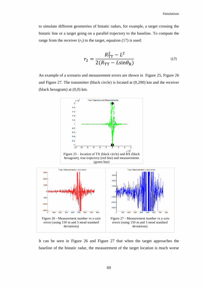
Simulations
69
to simulate different geometries of bistatic radars, for example, a target crossing the
bistatic line or a target going on a parallel trajectory to the baseline. To compute the
range from the receiver (r2) to the target, equation (17) is used:
(17)
An example of a scenario and measurement errors are shown in Figure 25, Figure 26
and Figure 27. The transmitter (black circle) is located at (0,200) km and the receiver
(black hexagram) at (0,0) km.
Figure 25 – location of TX (black circle) and RX (black
hexagram), true trajectory (red line) and measurements
(green line)
Figure 26 - Measurement number vs x-axis
errors (using 150 m and 3 mrad standard
deviations)
Figure 27 - Measurement number vs y-axis
errors (using 150 m and 3 mrad standard
deviations)
It can be seen in Figure 26 and Figure 27 that when the target approaches the
baseline of the bistatic radar, the measurement of the target location is much worse

Simulations
70
than when it is far from the baseline. For this example, a range standard deviation of
150 m and an azimuth standard deviation of 3 mrad are used.
Script04b.m file is a script which uses new classes: “TRadar” (instead of “Radar”)
and “TEnvironment” and “TTarget”. Those new classes were created to make the
scripts (Matlab code) easier to read, understand and maintain. Besides, they will help
to make changes to the parameters of the simulations easier. When using
Script04b.m, it is possible to simulate different geometries of one monostatic radar
or one bistatic radar. In addition, the new class “TRadar” provides the new
functionality of having range and angle measurements standard deviations that vary
according to SNR. It means that if the target is far from the radar, the SNR will be
small and hence the standard deviation of the measurements will be bigger.
Equations (18) and (19) (pages 69 and 70 of [74]) show how the standard deviations
are calculated (range and azimuth standard deviations, respectively), where N is the
number of pulses integrated. SNR is calculated using the radar range equation (12).
(18)
(19)
Some examples of graphics generated from script04b.m are found in Figure 28,
Figure 29 and Figure 30 for the monostatic case and Figure 31, Figure 32 and Figure
33 for bistatic case (when the target is parallel to the baseline).
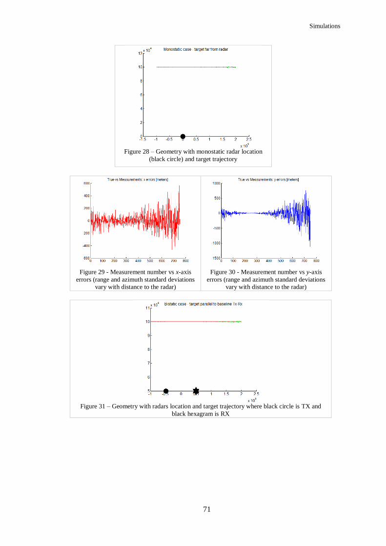
Simulations
71
Figure 28 – Geometry with monostatic radar location
(black circle) and target trajectory
Figure 29 - Measurement number vs x-axis
errors (range and azimuth standard deviations
vary with distance to the radar)
Figure 30 - Measurement number vs y-axis
errors (range and azimuth standard deviations
vary with distance to the radar)
Figure 31 – Geometry with radars location and target trajectory where black circle is TX and
black hexagram is RX

Simulations
72
Figure 32 - Measurement number vs x-axis
errors (range and azimuth standard deviations
vary with distance to the radar)
Figure 33 - Measurement number vs y-axis
errors (range and azimuth standard deviations
vary with distance to the radar)
For the examples in Figure 28 to Figure 33, the radar and target characteristics are:
Radar Power: 1.5MW
Frequency: 8 GHz
PRF: 1500 Hz
Beam width: 5 degrees
Pulse Width: 0.7 μs and Range Resolution: 105 meters
Antenna rotation: 30 RPM, pulses per beam width: 27 and Sampling rate: 2
seconds (change in TRadar.m and script04b.m)
Antennas gain: 45 dB and Noise figure: 3 dB
target RCS is 0.1 m2 and x-velocity is 200 m/s (in TEnvironment.m)
Following, next script (script10.m) uses a new class named “TghFilter” which
implements a g-h filter. The g-h filter implemented is a version of a “Critically
Damped Filter” [50] where the values of g and h are a function of θ and θ can be a
value between 0 and 1, where values close to 0 mean that the filter trusts more on
recent measurements and values close to 1 mean that the filter trusts more on
historical measurements. The values of g and h are according to equation (20), once
θ is defined.
(20)

Simulations
73
The simulation considers a target flying on a straight trajectory with constant
velocity and the value of θ changes during the filtering process from an initial value
of 0.10 (recent measurements are more important) to a maximum value of more than
0.90 (historical measurements are more important). The values were chosen after
some simulations to assess the performance of the g-h filter. The filter algorithm can
be used to filter the measurements performed either by a monostatic or a by a bistatic
radar. Still using script10.m file, it generates a series of graphs that depict, for each
geometry (monostatic or different bistatic geometries), measurements, filtered
measurements of position and velocity of the target and also, in the bistatic
configurations, bistatic angle is presented. Below, there is an example of a simulation
using bistatic geometry.
Figure 34 – Geometry with radars location and
target trajectory where black circle is TX and
black hexagram is RX
Figure 35 – Bistatic angle along the target
trajectory
Figure 36 – x-position of the target vs x-axis
errors
Figure 37 – x-position of the target vs y-axis
errors

Simulations
74
Figure 38 - x-position of the target vs x-axis
errors after tracking filter
Figure 39 - x-position of the target vs y-axis
errors after tracking filter
Figure 40 – x-position of the target vs x-axis (red) and y-axis (blue) estimated velocity
The main objective of script11 file series (script11a.m, script11b.m, and so on) is to
make use of data fusion in scenarios where more than one radar (monostatic or
bistatic) are used in order to improve the resulting measurements or filtered
measurements. The data fusion can be done, for example, in two different ways:
a) by applying weight to the measurements according to SNR and then perform
a weighted mean of the measurements or the filtered measurements to have
the final result or
b) by applying weight to the measurements according to SNR to select the best
measurement or filtered measurement to be used.
Function wmean() is used to perform the chosen method. In this research, method (a)
is chosen for the simulations.
In all script11 files, the sampling rate is 4 seconds and beam width is 3 degrees.
In the specific case where the SNR is high because the target is near or crossing the
baseline of a bistatic radar, the weight of the measurements must be reduced when

Simulations
75
the bistatic angle lies in the range between 145-180 degrees since the measurements
in this region are not very accurate as it can be seen in Figure 36 and Figure 37.
Figure 41, Figure 42 and Figure 43, present one example of fusion of data
(measurements or tracks) in a scenario with 2 monostatic radars (using script11.m).
The resulting track is the same if comparing the algorithm that fuse the tracks (Figure
42) with the algorithm that fuse the measurements before applying the tracking filter
(Figure 43).
Figure 41 - Geometry with radars location and target trajectory (red) where green and cyan
circles are monostatic radars. Green and cyan dots represent measurements from each radar
respectively
Figure 42 – Individual tracks (green and cyan
dots) and fused track (black line)
Figure 43 – Fused measurements (yellow) and
track (black line)
The last script of this series, script11z.m, generates graphs to compare the use of one
monostatic radar with power of 1.5 MW and the use of 4 monostatic radars of 375
kW on a network. The following figures depict both scenarios.

Simulations
76
Figure 44 - Geometry with radar location,
target trajectory (red) and measurements
(green). The black circle is the monostatic
radar
Figure 45 - Geometry with radars location
where green, blue, red and magenta circles are
monostatic radars and the same colours of lines
represent their respective measurements
Figure 46 – Track when only one radar (1.5
MW) is used
Figure 47 – Fusion of tracks from each radar (4
radars of 375 kW)
It can be observed that in Figure 46, the errors in the beginning of the trajectory are
bigger than in the Figure 47. However in the geometry of Figure 46 the track is more
stable until 200 km whereas in Figure 47 the track starts do diverge from 100 km.
So far, all scripts performed just one run of the simulation. The results show a rough
idea about how tracking accuracy varies when geometries or radar characteristics are
changed. Nevertheless, due to the random nature of the errors it is appropriate to run
each simulation many times in order to see and understand the pattern of the errors.
The next series of scripts, script12 files (script12.m, script12a.m, and so on) perform
the same tasks as the script11 series but now making use of Monte Carlo Simulation
techniques. Thus, for each geometry, many Monte Carlo runs are performed before
generating the graphs. For instance, for the same scenario depicted in Figure 46 and
Figure 47, the results would be according to the Figure 48 and Figure 49 (with 100
simulations runs) and they show that both geometries have similar results apart from

Simulations
77
the beginning of the trajectory where the netted monostatic geometry performs better
(script12z.m).
Figure 48 - Track when only one radar (1.5
MW) is used
Figure 49 - Fusion of tracks from each radar (4
radars of 375 kW)
In script13.m, a new filter, g-h-k filter is programmed and assessed. It is again a
version of a “Critically Damped Filter” [50] where the values of g, h and k are a
function of θ and θ can be a value between 0 and 1, where values close to 0 mean
that the filter should trust more on recent measurements and values close to 1 mean
that the filter should trust more on historical measurements. The values of g, h and k
are defined according to equation (21).
(21)
Similarly to the g-h filter, this g-h-k filter also starts with the value of θ = 0.10 and
then increases gradually up to 0.90 or more, for example. The need of using a g-h-k
filter comes from the idea of performing the simulations using a target that
manoeuvres. A sinusoidal trajectory is used to see how the g-h-k filter performs. The
following figures show an example of 2 monostatic radars used to track such a target.

Simulations
78
Figure 50 - Geometry with radars location,
target trajectory (red sinusoidal) and
measurements (green/blue) from each
monostatic radar (green and blue circles)
Figure 51 – Tracking (black line) using a g-h-k
filter after doing fusion of measurements
(yellow)
The track result from g-h-k filter (Figure 51) is better than the result from g-h filter
depicted in the Figure 52.
Figure 52 - Tracking (black line) after doing fusion of measurements (yellow) using a g-h filter
For the script20.m, the sampling time is changed to 2 seconds and the beam width
changed to 5 degrees. The main objective of script20.m is to perform in the same
scenarios of scrip10.m with a target moving on a sinusoidal trajectory to assess the g-
h-k filter. The sinusoidal trajectory simulated has a constant velocity on the x-axis
and a non-constant velocity and acceleration in the y-axis.
Figure 53 shows the estimate velocity using a g-h filter and Figure 54 shows the
estimate velocity using a g-h-k filter. The use of g-h-k filter improved the estimation
of y-velocity.

Simulations
79
Figure 53 – Estimated y-velocity (blue line)
using a g-h filter. Black line is the true
velocity. Estimated x-velocity is illustrated by
the red line (constant 200 m/s)
Figure 54 – Estimated y-velocity (blue line)
using a g-h-k filter. Black line is the true
velocity. Estimated x-velocity is illustrated by
the red line (constant 200 m/s)
Although, so far, all the scripts to track targets uses g-h or g-h-k filters (Figure 53
and Figure 54), a Kalman Filter has been developed and the result can be seen in
Figure 55.
Figure 55 – Estimated velocity (blue line) using a g-h-k filter. Black line is the true velocity
The use of Kalman Filter brings an improvement in the estimated velocities and thus
to estimated position of the target.
For the next (and last) 2 scripts (script30.m and script30a.m), only Kalman filter is
considered. Kalman Filter uses more computational resources but as long as it is not
a limitation for the simulations and for the current computer power available in the
market and its results are considerably better, this will be the filter used for the
analysis of this thesis. Therefore, the main simulations and results are performed
using script30.m and script30a.m.
This section has explained the methodology and has built step-by-step the important
concepts to be used by script30.m and script30a.m as the main simulations.

Simulations
80
6.3 Algorithms
Choosing the right filtering algorithm to be used in the simulations depends on
specific characteristics of the problem. The initial idea was to perform simulations
using a target whose trajectory was linear, on a straight line and with a constant
speed. In this scenario, using a g-h filter was enough to achieve acceptable results. A
Critically Damped g-h filter [50] has been used, where the variable θ was varying
from some value close to 0 to some value close to 1 during the trajectory of the
target.
In a scenario where some acceleration was considered (for example, when the target
has a sinusoidal trajectory with constant x-velocity and some acceleration in y-axis),
the use of a g-h-k filter was more appropriate. Although the filter considers a
constant acceleration and the target had some non-constant acceleration, the filter
performed well. Once more, the g-h-k filter that has been implemented was the
Critically Damped g-h-k filter where θ varied the same way as in the g-h version.
In a situation where computer resources are limited, the use of g-h-k filter with some
tuning in the θ variable would be enough for some target trajectories. However,
nowadays, computer power is not a problem if compared to 50 years ago when the
Kalman Filter was published [20]. Therefore, a Kalman Filter was implemented (3-
state, position, velocity and acceleration) for the main simulations of this research
and, because of that, it is possible to achieve better results when the target
manoeuvres.
A brief explanation about each filter used is given in the next sections. In addition,
some explanation on how the measurements are simulated is presented.
6.3.1 Simulated Measurements
The simulated measurements consider the real position of the target according to its
trajectory (straight line, sinusoidal or spiral). From the real 2D position (x,y) of the
target, a true measurement of range and bearing angle (azimuth) is calculated with
respect to the radar position (receiver) using Cartesian-to-Polar conversion. Then
some noise is added to the range and azimuth measurements. This noise is a white

Simulations
81
noise, with zero mean and with variances that varies according to SNR. SNR is
calculated according to the radar equation, which depends on many variables such as
Transmitter Power, wavelength, antenna gains, RCS, etc. The same SNR is used by
the fusion algorithm in order to measure how accurate or how good is the
measurement. In bistatic measurements, this weight factor is reduced when the
bistatic angle is close to 180 degrees. Therefore, the sequence below is performed in
order to simulate a measurement:
1) In monostatic cases, from true x-y position, use Cartesian-to-Polar conversion
and find true range and azimuth (R and θ);
2) In the case of bistatic geometries, from true x-y position, the distances
transmitter-target and target-receiver are calculated and then summed to find RT.
θ in the bistatic case is the bearing angle (θR) with respect to the vertical axis
(see Figure 12 and equation (1))
3) From the true range, calculate SNR (RCS is considered to be constant in all
cases, monostatic or bistatic, regardless of aspect angle, geometry and so on)
using radar range equation;
4) From SNR, calculate standard deviations for range and azimuth measurements
[74]. See equations (18) and (19);
5) Calculate measurement plus noise (range plus noise and azimuth plus noise) and
6) Use SNR to weigh the importance of a measurement (to be used in measurement
fusion procedure).
6.3.1.1 Fusion of measurements
SNR is used to calculate standard deviations for range and azimuth and also is the
information used to weigh the measurements so that the fusion process (weighted
average of measurements and variances) can give more importance to measurements
with larger SNR. Nonetheless, when the target is close to the baseline of a bistatic
radar which means that the bistatic angle is close to 180 degrees, its measurements
can get worse and it is difficult to measure where the target is lying in or near the
baseline. Therefore, the decision was to model the measurements from a bistatic

Simulations
82
radar to be less important dividing the SNR by a factor according to equation (22)
when the bistatic angle has a value between 145 and 180 degrees.
(22)
6.3.2 Critically Damped g-h filter
The Critically Damped g-h filter used in this research is a slightly different version
from the one reported in [50]. In this research, it has been realized that varying the
parameter θ from small values (0.10) to higher values (more than 0.90) during the
process of tracking resulted in some improvement in the tracking errors. So, the
following equations are used to estimated position and velocity:
1) First, start with a small θ, for example, 0.10
2) Calculate g and h using equation (20)
3) Calculate estimate position and velocity using the measurements and the
following equations [50]
, where T is the sampling
interval, yn is the nth
-measurement and * means estimate
means the estimated velocity for step n+1, using
measurements until step n
(23)
(24)
4) Increase θ (until a maximum of about 0.90) by a small amount, for example,
0.05 and go back to step 2.
6.3.3 Critically Damped g-h-k filter
This filter is similar to the previous one and the steps to calculate the estimate
position, velocity and acceleration are similar, except that now there is an extra
parameter, k.
1) First, start with a small θ, for example, 0.10

Simulations
83
2) Calculate g, h and k using equation (21)
3) Calculate estimate position, velocity and acceleration using the measurements
and the following equations [50].
(25)
(26)
(27)
(28)
(29)
(30)
4) Increase θ (until a maximum of about 0.90) by a small amount, for example,
0.05 and go back to step 2.
6.3.4 Kalman Filter (KF)
The KF algorithm used in this research is based on [50]. The algorithm to perform
the tracking using KF is as follows:
1) Set ϕ which is the transition matrix. It is a 2x2 matrix (for 2-state filter) or a 3x3
matrix (for 3-state filter)
or (31)

Simulations
84
2) Set M, the measurement matrix, which is 2(measurements)x4 for a 2-state filter
or 2(measurements)x6 for a 3-state filter
or
(32)
3) Set S0, the covariance of prediction matrix (4x4 for 2-state filter or 6x6 matrix
for 3-state filter). The number 108 was chosen to be very large in order to make
the filter, at the beginning, to trust more on measurements and not on predictions
or (33)
4) Set Q, the dynamic noise covariance matrix
, where Ux and Uy are
and
, where
and
maxAccelX, maxAccelY and B are set according to page 66 of
[50]
(34)
5) With the measurement, calculate R, the measurement covariance vector (see
page 179 of [74])
, where
θ
,
θ and
θ , where
(35)
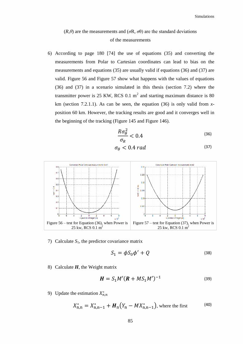
Simulations
85
(R,θ) are the measurements and (σR, σθ) are the standard deviations
of the measurements
6) According to page 180 [74] the use of equations (35) and converting the
measurements from Polar to Cartesian coordinates can lead to bias on the
measurements and equations (35) are usually valid if equations (36) and (37) are
valid. Figure 56 and Figure 57 show what happens with the values of equations
(36) and (37) in a scenario simulated in this thesis (section 7.2) where the
transmitter power is 25 KW, RCS 0.1 m2 and starting maximum distance is 80
km (section 7.2.1.1). As can be seen, the equation (36) is only valid from x-
position 60 km. However, the tracking results are good and it converges well in
the beginning of the tracking (Figure 145 and Figure 146).
(36)
(37)
Figure 56 – test for Equation (36), when Power is
25 kw, RCS 0.1 m2
Figure 57 – test for Equation (37), when Power is
25 kw, RCS 0.1 m2
7) Calculate S1, the predictor covariance matrix
(38)
8) Calculate H, the Weight matrix
(39)
9) Update the estimation
, where the first (40)

Simulations
86
prediction is based on the first measurement
10) Update S0
(41)
11) Calculate the new prediction
(42)
12) Go back to step 5

Results
87
7 Results
When all the scripts are run, some assumptions about the radar parameters have to be
made. First of all, it is a two-dimensional space where radars and target have their
positions established in Cartesian coordinates (x and y coordinates). The
measurements are in Polar coordinates (range or total range, and bearing angle) and
the sampling rate of the measurements is 2.5 seconds (unless mentioned differently
for a specific simulation), considering an antenna rotation of 24 RPM (TRadar.m).
The measurements are then transformed to Cartesian coordinates in order to be
filtered by the Kalman Filter. The target flies in a straight line with a constant
velocity or for the complex scenarios, the target flies in a spiral-like trajectory. The
standard deviations of range and bearing angle measurements are functions of the
range to the target. SNR is calculated using the Radar Equation (or Bistatic Radar
Equation). Table 2 shows a summary of the radar parameters.
Table 2 – Main radar parameters used in the simulations and some other related information
Coordinates Two-dimensional
Measurements Polar coordinates (range, bearing
angle)
Tracking Cartesian Coordinates (x,y)
Antenna Rotation 24 RPM, hence sampling rate 2.5 sec
Tracking Filter Kalman Filter (KF)
Target trajectory
Straight line with constant velocity or
spiral with non-constant x and y
velocity and acceleration

Results
88
Probability of Detection (PD) 100%
Probability of False Alarm (PFA) 0%
Range and azimuth standard
deviation Function of Range, hence SNR
SNR Calculated with Radar Equation
Transmitter Power 25 kW (or a fraction, according to the
geometry)
Antenna Gain (TX and RX) 45 dB
Radar Frequency 9.41 GHz, hence λ=3.19 cm
Radar Cross Section (perfectly
conducting sphere)
10 m2 or 0.1 m
2, hence sphere radius
of 1.78m or 17.8 cm
Pulse width 0.7 micro seconds, hence range
resolution = 105m
Bandwidth (B) =
1.4 MHz
Noise figure 3 dB
Losses (L in Equation (9)) 0 dB
Beam width 2 degrees
Pulse Repetition Frequency (PRF) 1 KHz
Unambiguous range 150 km
Pulses per beam width
13
Horizon (considering H1, height of
antenna 10 meters and H2
, where d is in
nautical miles and H1 and H2 are in
feet
25 km, if H2=10 meters (ship)
422 km, if H2=10 km (aircraft)
Different geometries and scenarios are exploited as measurements and filtering are
performed in each case. The main idea is to make comparisons of the true trajectory
against measurements and filtered measurements when the target crosses different
geometries of radar (monostatic, netted monostatic, bistatic or multistatic). In more
sophisticated scenarios where more than one radar is working cooperatively on a
network (netted monostatic radars or multiple bistatic pairs comprising a multistatic

Results
89
radar), a data fusion algorithm is used in order to combine the measurements (or
filtered measurements).
7.1 Measurements Results
In these simulations, script30.m is used and, for each scenario, two different target
Radar Cross Section is used, 10 m2 and 0.1 m
2 (change in TEnviroment.m).
7.1.1 Monostatic
7.1.1.1 Target RCS 10 m2
In this first simulation, only one monostatic radar of 25 kW is being used to perform
the measurements on the target. The radar is located at position (0,0) and the target is
flying from (-100,100) km with an x-velocity of 250 m/s (TEnvironment.m). The
measurements are performed during 1000 seconds every 2.5 seconds (antenna
rotation is 24 RPM). Figure 58 shows the geometry where a black circle represents
the monostatic radar, the green dots are the measurements and the red line is the true
trajectory. Figure 59 and Figure 60 depict the measurements errors in x and y-axis
respectively. Figure 61 denotes how SNR and bistatic angle (on a bistatic
configuration) changes with x-position of the target. And finally, Figure 62 shows the
range (blue) and azimuth (green) measurements standard deviations. In this scenario,
note that the errors in y-axis (Figure 60) become very good (less than ± 50m)
between x-target locations -50 km and 50 km. This is due to the fact that range
measurement standard deviation is around 1m. The x-position errors do not improve
so much even though the azimuth measurement standard deviation is also small
(about 0.5 mrad). This is because at a distance of 100 km, even a small error in the
measurement of the bearing angle (0.5 mrad) can affect the results and the location of
the target is less accurate.

Results
90
Figure 58 – Location of TX/RX (monostatic radar with 25 kW), true trajectory (red line) and
measurements (green dots)
Figure 59 - x-position vs x-axis errors (1 radar
25 kW)
Figure 60 - x-position vs y-axis errors (1 radar
25 kW)
Figure 61 – x-position vs SNR (blue line) – 1
radar 25 kW
Figure 62 – x-position vs [range stddev(blue)
and azimuth stddev (green)] – 1 radar 25 kW
The same geometry is used in the following figures, but using a radar with 4 times
less power, 6.25 kW. As it was expected the errors are larger as SNR decreases and
standard deviations get worse.

Results
91
Figure 63 - x-position vs x-axis errors (1 radar
6.25 kW)
Figure 64 - x-position vs y-axis errors (1 radar
6.25 kW)
Figure 65 – x-position vs SNR (blue line) – 1
radar 6.25 kW
Figure 66 – x-position vs [range stddev(blue)
and azimuth stddev (green)] – 1 radar 6.25 kW
In following scenario, the radar is located on the way of the target at (0,100) km.
Now, it is possible to see x-position errors are much better than y-position errors,
again due to the fact that at a location 100 km from the radar, even such a small
azimuth measurement standard deviation (0.4 mrad) can bring an error of about ±
80m when the target is initiating its trajectory at (-100,100) km.
Figure 67 – Location of TX/RX (monostatic radar with 25 kW), true trajectory (red line) and
measurements (green dots)

Results
92
Figure 68 - x-position vs x-axis errors (1 radar
25 kW)
Figure 69 - x-position vs y-axis errors (1 radar
25 kW)
Figure 70 – x-position vs SNR (blue line) – 1
radar 25 kW
Figure 71 – x-position vs [range stddev(blue)
and azimuth stddev (green)] – 1 radar 25 kW
The figures below depict the same scenario with 4 times less transmitter power (6.25
kW). As shown earlier, the errors are larger because of the resulting smaller SNR and
worse standard deviations. As expected, the errors are 2 times larger with the
reduction on power of 4 times. This happens, because SNR reduces 4 times (due to
radar equation (9)) and as a consequence, because of the square root factor of
equations (18) and (19), standard deviations (range and azimuth) increase by a factor
of 2.

Results
93
Figure 72 – Location of TX/RX (monostatic radar with 6.25 kW), true trajectory (red line) and
measurements (green dots)
Figure 73 - x-position vs x-axis errors (1 radar
6.25 kW)
Figure 74 - x-position vs y-axis errors (1 radar
6.25 kW)
Figure 75 – x-position vs SNR (blue line) – 1
radar 6.25 kW
Figure 76 – x-position vs [range stddev(blue)
and azimuth stddev (green)] – 1 radar 6.25 kW
7.1.1.2 Target RCS 0.1 m2
Now, the same trajectory crossing the same geometries as in section 7.1.1.1, but the
target has RCS of 0.1 m2 (TEnvironment.m). It can be seen in all figures in this
section, that comparing to the figures in the previous section, the reduction on RCS
from 10 m2 to 0.1 m
2, made the errors to increase 10 times. The reduction on RCS by
a factor of 100 (20 dB), makes SNR to reduce 100 times as well, and due to the

Results
94
square root factor of equations (18) and (19), standard deviations increase by a factor
of 10.
Figure 77 - Location of TX/RX (monostatic radar with 25 kW), true trajectory (red line) and
measurements (green dots)
Figure 78 - x-position vs x-axis errors (1 radar
25 kW)
Figure 79 - x-position vs y-axis errors (1 radar
25 kW)
Figure 80 – x-position vs SNR (blue line) – 1
radar 25 kW
Figure 81 – x-position vs [range
stddev(blue) and azimuth stddev (green)] – 1
radar 25 kW
In the next scenario, Figure 82 to Figure 86 are equivalent to Figure 67 to Figure 71,
with the target having an RCS of 0.1 m2.

Results
95
Figure 82 – Location of TX/RX (monostatic radar with 25 kW), true trajectory (red line) and
measurements (green dots)
Figure 83 - x-position vs x-axis errors (1 radar
25 kW)
Figure 84 - x-position vs y-axis errors (1 radar
25 kW)
Figure 85 – x-position vs SNR (blue line) – 1
radar 25 kW
Figure 86 – x-position vs [range stddev(blue)
and azimuth stddev (green)] – 1 radar 25 kW
7.1.2 Bistatic
In the bistatic scenarios depicted in the next sections, bistatic radars are represented
by a TX (black circle) and a RX (black hexagram). The target has an x-velocity of
250 m/s and the measurements are performed during 1000 seconds every 2.5
seconds.

Results
96
7.1.2.1 Target RCS 10 m2
Figure 87 shows the geometry with TX and RX separated by 100 km which is the
baseline. The target is moving horizontally and parallel to the baseline.
Figure 87 - Location of TX and RX (bistatic radar with TX 25 kW), true trajectory (red line) and
measurements (green dots)
Figure 88 - x-position vs x-axis errors (1 TX 25
kW)
Figure 89 - x-position vs y-axis errors (1 TX 25
kW)
Figure 90 – x-position vs [SNR (blue line) and
bistatic angle (green line) – 1 TX 25 kW
Figure 91 – x-position vs [range stddev(blue)
and azimuth stddev (green)] – 1 TX 25 kW
In the example below, the TX still have 25 kW power but the baseline is 200 km and
is perpendicular to the target trajectory which crosses the baseline. Observing Figure
93, Figure 94 and Figure 95 it can be seen that when bistatic angle gets close to 180

Results
97
degrees, the measurements errors get much worse, although SNR is higher (Figure
95) in this region. This is due to equation (1).
Figure 92 - Location of TX and RX (bistatic radar with TX 25 kW), true trajectory (red line) and
measurements (green dots)
Figure 93 - x-position vs x-axis errors (1 TX 25
kW)
Figure 94 - x-position vs y-axis errors (1 TX 25
kW)
Figure 95 – x-position vs [SNR (blue line) and
bistatic angle (green line) – 1 TX 25 kW
Figure 96 – x-position vs [range stddev(blue)
and azimuth stddev (green)] – 1 TX 25 kW
The next 2 scenarios show what happens with the measurements errors when the
power of TX is reduced by a factor of 4.
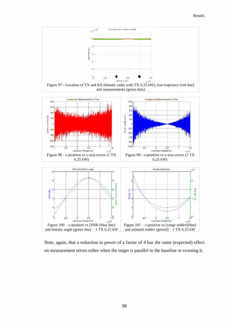
Results
98
Figure 97 - Location of TX and RX (bistatic radar with TX 6.25 kW), true trajectory (red line)
and measurements (green dots)
Figure 98 - x-position vs x-axis errors (1 TX
6.25 kW)
Figure 99 - x-position vs y-axis errors (1 TX
6.25 kW)
Figure 100 – x-position vs [SNR (blue line)
and bistatic angle (green line) – 1 TX 6.25 kW
Figure 101 – x-position vs [range stddev(blue)
and azimuth stddev (green)] – 1 TX 6.25 kW
Note, again, that a reduction in power of a factor of 4 has the same (expected) effect
on measurement errors either when the target is parallel to the baseline or crossing it.

Results
99
Figure 102 - Location of TX and RX (bistatic radar with TX 6.25 kW), true trajectory (red line)
and measurements (green dots)
Figure 103 - x-position vs x-axis errors (1 TX
6.25 kW)
Figure 104 - x-position vs y-axis errors (1 TX
6.25 kW)
Figure 105 – x-position vs [SNR (blue line)
and bistatic angle (green line) – 1 TX 6.25 kW
Figure 106 – x-position vs [range stddev(blue)
and azimuth stddev (green)] – 1 TX 6.25 kW
7.1.2.2 Target RCS 0.1 m2
Now, the same trajectory crossing the same bistatic geometries as in section 7.1.2.1,
but the target has RCS of 0.1 m2. It can be seen in all figures in this section, that
comparing to the figures in the previous section, the reduction on RCS from 10 m2 to
0.1 m2, made the errors to increase 10 times. The reduction on RCS by a factor of

Results
100
100 (20 dB), makes SNR to reduce 100 times as well, and due to the square root
factor of equations (18) and (19), standard deviations increase by a factor of 10.
Figure 107 - Location of TX and RX (bistatic radar with TX 25 kW), true trajectory (red line)
and measurements (green dots)
Figure 108 - x-position vs x-axis errors (1 TX
25 kW)
Figure 109 - x-position vs y-axis errors (1 TX
25 kW)
Figure 110 – x-position vs [SNR (blue line)
and bistatic angle (green line) – 1 TX 25 kW
Figure 111 – x-position vs [range stddev(blue)
and azimuth stddev (green)] – 1 TX 25 kW
Figure 112 to Figure 116 present the scenario where the target crosses the baseline of
the bistatic radar.

Results
101
Figure 112 - Location of TX and RX (bistatic radar with TX 25 kW), true trajectory (red line)
and measurements (green dots)
Figure 113 - x-position vs x-axis errors (1 TX
25 kW)
Figure 114 - x-position vs y-axis errors (1 TX
25 kW)
Figure 115 – x-position vs [SNR (blue line)
and bistatic angle (green line) – 1 TX 25 kW
Figure 116 – x-position vs [range stddev(blue)
and azimuth stddev (green)] – 1 TX 25 kW
7.1.3 Multistatic (1 x N)
In the multistatic scenarios depicted below, the main purpose is to show the results
from the fusion algorithm when performed using measurements from 2 radars (for
example, 2 bistatic radars). For multistatic scenarios, only targets with RCS=0.1 m2
are considered as it is the main focus of this research.

Results
102
Figure 117 to Figure 127 show a geometry where there is only 1 TX (25 kW) and 2
RXs, and the target has RCS=0.1 m2. The black circle is the TX and the green and
magenta hexagrams are RXs. Thus, the target is crossing the baseline of a bistatic
radar (black/green pair) and going on a parallel line of another bistatic radar
(black/magenta pair).
Figure 117 - Location of 1 TX 25 kW (black circle) and 2 RXs (green and magenta hexagrams),
true trajectory (red line) and measurements (green and magenta dots)
Figure 118 - x-position vs x-axis errors (1 TX
25 kW) – when crossing baseline
Figure 119 - x-position vs y-axis errors (1 TX
25 kW) – when crossing baseline
Figure 120 - x-position vs x-axis errors (1 TX
25 kW) – when parallel to baseline
Figure 121 - x-position vs y-axis errors (1 TX
25 kW) – when parallel to baseline

Results
103
Figure 122 - x-position vs x-axis errors (1 TX
25 kW) – after fusion procedure
Figure 123 - x-position vs y-axis errors (1 TX
25 kW) – after fusion procedure
Figure 124 – x-position vs SNR (for each
radar)
Figure 125 – x-position vs bistatic angle (for
each radar)
Figure 126 – x-position vs Range std dev (for
each radar)
Figure 127 – x-position vs Azimuth std dev
(for each radar)
7.1.4 Multistatic (M x 1)
Figure 128 to Figure 138 depict a geometry where there is only 1 RX and 2 TXs (of
12.5 kW each). The black hexagram is the RX and the green and magenta circles are
the TXs, like the previous scenario. Thus, the target is crossing the baseline of a
bistatic radar (black/green pair) and going on a parallel line of another bistatic radar
(black/magenta pair).

Results
104
Figure 128 - Location of 2 TXs 12.5 kW (green and magenta circles) and 1 RX (black
hexagram), true trajectory (red line) and measurements (green and magenta dots)
Figure 129 - x-position vs x-axis errors (1 TX
12.5 kW) – when crossing baseline
Figure 130 - x-position vs y-axis errors (1 TX
12.5 kW) – when crossing baseline
Figure 131 - x-position vs x-axis errors (1 TX
12.5 kW) – when parallel to baseline
Figure 132 - x-position vs y-axis errors (1 TX
12.5 kW) – when parallel to baseline

Results
105
Figure 133 - x-position vs x-axis errors (2 TXs
12.5 kW) – after fusion procedure
Figure 134 - x-position vs y-axis errors (2 TXs
12.5 kW) – after fusion procedure
Figure 135 – x-position vs SNR (for each
radar)
Figure 136 – x-position vs bistatic angle (for
each radar)
Figure 137 – x-position vs Range std dev (for
each radar)
Figure 138 – x-position vs Azimuth std dev
(for each radar)
In this scenario, there are 2 TXs of half of the power of the scenario where there was
1 TX (section 7.1.3). So, instead of having 2 pairs of bistatic radars with a 25 kW
TX, there are 2 pairs of bistatic radars with 12.5 kW TXs. But, because of the square
root factor in equations (18) and (19), the errors increased about 1.4 times if
compared to the scenario in 7.1.3.
Therefore, although it seems to be better to use a configuration with 1 TX (25 kW)
and 1 RX instead of 2 TXs (12.5 kW) and 1 RX, there is an advantage when using

Results
106
the latter that, if one TX is lost (in military scenarios, it is more likely that a TX is
located and thus destroyed) the whole system can still work (with some loss in
performance).
7.1.5 Measurements Summary Table
Section 7.1 presents a series of simulations performing measurements in different
scenarios, including monostatic, bistatic and multistatic ones. Table 3 presents a
summary from the measurements simulations in monostatic geometries. This is to
illustrate how different parameters on the geometry or target can affect the
measurements errors.
Table 3 – Measurements Summary for monostatic geometries – measurement errors during the
trajectory of the target in different configurations, changing location and transmit power of the radar
and target RCS
Geometry Errors in x-axis measurement (m) Errors in y-axis measurement (m)
x=-50
km
x=0
km
x=50 km x=100
km
x=-50
km
x=0
km
x=50
km
x=100 km
(1) Monostatic
(25 kW) far 150 100 150 200 75 5 75 200
(2) Monostatic
(6.25 kW) far 300 200 300 400 150 10 150 400
(3) Monostatic
(25 kW) 0.75 0 0.75 3 10 0 10 100
(4) Monostatic
(6.25 kW) 1.5 0 1.5 6 20 0 20 200
(5) Monostatic
(25 kW) far
RCS=0.1 m2
1500 1000 1500 2000 750 50 750 2000
(6) Monostatic
(25 kW) RCS=0.1 m2
7.5 0 7.5 30 100 0 100 1000
From line (1) to line (2), TX power is reduced from 25 kW to 6.25kW and it results
in an increase on errors by a factor of 2. The same happens from line (3) to line (4)
but, in those lines, TX is on the target trajectory and thus the errors are significantly
smaller. Line (5) is compared to line (1), where in line (5) RCS of the target is
reduced by a factor of 100 (from 10 m2 to 0.1 m
2) which results in increasing of the
errors by a factor of 10. The same situation occurs when comparing line (6) to line
(3).

Results
107
Next table, Table 4, depicts a summary from the measurements simulations in
bistatic geometries and its purpose is to demonstrate that the same assumptions for
the errors are valid.
Table 4 - Measurements Summary for bistatic geometries – measurement errors during the trajectory
of the target in different configurations, changing location and transmit power of the radar and target
RCS
Geometry Errors in x-axis measurement (m) Errors in y-axis measurement (m)
x=-50
km
x=0
km
x=50 km x=100
km
x=-50
km
x=0
km
x=50
km
x=100 km
(1) Bistatic
(25 kW) 200 125 175 225 150 50 0 100
(2) Bistatic
(25 kW) crossing
4 4 4 300 300 400
(3) Bistatic (6.25 kW)
400 250 350 450 300 100 0 200
(4) Bistatic (6.25 kW)
crossing
8 8 8 600 600 800
(5) Bistatic
(25 kW)
RCS=0.1 m2
2000 1250 1750 2250 1500 500 0 1000
(6) Bistatic
(25 kW) RCS=0.1 m2
crossing
40 40 40 3000 3000 4000
As an example, from Table 4, line (1) compared with line (3) has an increase in the
errors by a factor of 2 due to the decrease in the power by a factor of 4. The same
happens between lines (2) and (4). And if RCS is decreased by a factor of 100, the
errors increase by a factor of 10 as can be seen observing lines (1) and (5) and also
lines (2) and (6).
For multistatic scenarios, Table 5 summarizes what is simulated in 7.1.3 and 7.1.4
when the radar networks are comprised by 1 TX (25 kW) and 2 RXs or 2 TXs (12.5
kW each) and 1 RX. Lines (1) and (4) depict the results from the bistatic pair whose
baseline the target is crossing and lines (2) and (5) show the results from the pair
whose baseline is parallel to the target trajectory. Lines (3) and (6) depict the results
after performing the fusion of the measurements from both pairs of bistatic radars.
Table 5 - Measurements Summary for multistatic geometries – measurement errors during the
trajectory of the target in 2 different configurations, one Multistatic (1 TX / 2 RXs) and the other one
Multistatic (2 TXs / 1 RX)

Results
108
Geometry
RCS=0.1 m2
Errors in x-axis measurement (m) Errors in y-axis measurement (m)
1 TX (25 kW)
and 2 RXs
x=-50
km
x=0
km
x=50 km x=100
km
x=-50
km
x=0
km
x=50
km
x=100 km
(1) Crossing
pair 40 40 50 3000 3000 4000
(2) Parallel pair 2500 2000 1500 1200 2000 1000 0 500
(3) Fused 800 1750 800 1000 2000 1000 1500 1500
2 TXs (12.5
kW each) and
1 RX
(4) Crossing
pair 50 50 70 4000 4000 5000
(5) Parallel pair 3000 2000 2000 3000 2000 1000 0 1500
(6) Fused 800 2000 1000 2000 3000 1000 2000 2000
Table 6 shows, for monostatic scenarios, how different is the maximum SNR which
affects how good measurement standard deviations are. Only scenarios where the
target is far from the monostatic radar are depicted.
Table 6 – Maximum SNR and Best Range/Azimuth standard deviation for monostatic scenarios
(target flying far from TX/RX)
Geometry Maximum SNR (dB) Best Range standard
deviation (meters)
Best Azimuth standard
deviation (mrad)
(1) Far Monostatic (25
kW) RCS=10 m2
20.5 at x=0 1 0.4
(2) Far Monostatic (6.25
kW) RCS=10 m2
14.5 at x=0 2 0.8
(3) Far Monostatic (25
kW) RCS=0.1 m2
0.5 at x=0 10 4
From line (1) to line (2), the total power is reduced by a factor of 4 and thus SNR is
also reduced by a factor of 4 (or 6 dB). Standard deviations are increased by a factor
of 2. From line (1) to line (3), the total power is still the same, but target RCS is
decreased by a factor of 100 (20 dB) and thus SNR is decreased by the same factor.
Standard deviations are increased by a factor of 10.
Table 7 depicts, for bistatic scenarios, the maximum SNR and their respective best
range and azimuth standard deviations. Again, the same conclusions from Table 6
are valid for Table 7 when comparing lines (1), (3) and (5) (target not crossing the
baseline) and then comparing lines (2), (4) and (6) (target that cross the baseline).
Table 7 - Maximum SNR and Best Range/Azimuth standard deviation for bistatic scenarios

Results
109
Geometry Maximum SNR (dB) Best Range standard
deviation (meters)
Best Azimuth standard
deviation (mrad)
(1) Far Bistatic (25 kW) RCS=10 m2
18.5 at x=50 km 1.3 0.5
(2) Crossing Bistatic (25 kW) RCS=10 m2
20.5 at x=0 km 1 0.4
(3) Far Bistatic (6.25 kW)
RCS=10 m2
12.5 at x=50 km 2.6 1
(4) Crossing Bistatic (6.25 kW) RCS=10 m2
14.5 at x=0 km 2 0.8
(5) Far Bistatic (25 kW) RCS=0.1 m2
-1.5 at x=50 km 13 5
(6) Crossing Bistatic (25 kW) RCS=0.1 m2
0.5 at x=0 km 10 4
Finally, Table 8 presents Maximum SNR and standard deviations for multistatic
scenarios.
Table 8 - Maximum SNR and Best Range/Azimuth standard deviation for multistatic scenarios
Geometry Maximum SNR (dB) Best Range standard
deviation (meters)
Best Azimuth standard
deviation (mrad)
Multistatic 1 x N (1 TX 25 kW and 2 RXs), RCS=0.1 m2 : 2 pairs of 25 kW bistatic radars
Crossing pair 0.5 at x=0 10 4
Parallel pair -1.5 at x=0 13 5
Multistatic N x 1 (2 TXs 12.5 kW and 1 RX), RCS=0.1 m2 : 2 pairs of 12.5 kW bistatic radars
Crossing pair -2.5 at x=0 15 5.5
Parallel pair -4.5 at x=0 18 7
The tables in this section present some quantitative values at certain points of the
trajectory and illustrate the influence of transmitter power and RCS in the results.
However, the graphics in previous sections depict a more thorough idea on how the
measurements behave along the whole trajectory for different geometries.
7.2 Tracking Results
As can be seen in Section 7.1, there are some scenarios where SNR have negative
values (in dB). In this section, it is assumed, for the purpose of this research, that the
minimum SNR in order to detect the target is 5 dB, which is a ratio of about 3.1. So,
for more realistic results, the radar nodes are positioned closer to the target, like
shown in Figure 139 and Figure 140 where the target starts to be tracked when it is
about 80 Km far from the radar and at this location the measurement have an SNR of
about 5 dB.

Results
110
Figure 139 - Location of TX/RX (monostatic
radar with 25 kW), true trajectory (red line)
and measurements (green dots)
Figure 140 - x-position vs SNR (blue line) – 1
radar 25 kW
The same is applied for spiral-like trajectories and Figure 141 to Figure 143 show the
trajectory, SNR and standard deviations according to x-position.
Figure 141 - Location of TX/RX (monostatic radar with 25 kW), true trajectory (red line) and
measurements (green dots)
Figure 142 - x-position vs SNR (blue line) – 1
radar 25 kW
Figure 143 - x-position vs [range stddev(blue)
and azimuth stddev (green)] – 1 radar 25 kW
Therefore, in this section, several geometries are presented with a target (target 1)
crossing with a horizontal constant speed of 250 m/s, during 600 seconds and then a
target (target 2) with a spiral trajectory with no constant velocity or acceleration

Results
111
during 1000 seconds. For all scenarios in this section, target RCS is 0.1 m2. Now,
script30a.m is run for each scenario and TEnvironment.m must be adapted in order
to use the correct target trajectories (comment some lines of code and uncomment
some others related to horizontal trajectories).
7.2.1 Target 1 (straight line)
In the next scenarios the target starts at (-75,25) km, flies on a straight line and for
each scenario, 100 simulation runs are performed in order to calculate the average
and standard deviation of the results.
7.2.1.1 Monostatic
This scenario represents a monostatic geometry where in Figure 144, the black circle
is the monostatic radar (TX/RX) with 25 kW, the red line is the true trajectory and
the green dots are the measurements. The following 2 figures (Figure 145 and Figure
146) represent the average position errors (red for x-axis and blue for y-axis) and ±1
standard deviation (green dotted line) after filtering. Finally, the last two figures of
this scenario (Figure 147 and Figure 148) show the average velocity errors (red for x-
axis and blue for y-axis) and ±1 standard deviation (green dotted line). Note that the
position errors in both axis are smaller than 20 meters after position x=-50 km and
velocity errors are smaller than 0.5 m/s from the same position.
Figure 144 – Location of TX/RX (monostatic radar with 25 kW), true trajectory (red line) and
measurements (green dots)

Results
112
Figure 145 - Average x-position error (red)
after tracking. Green lines depict ±1 standard
deviation
Figure 146 - Average y-position error (blue)
after tracking. Green lines depict ±1 standard
deviation
Figure 147 - Average x-velocity error (red)
after tracking. Green lines depict ±1 standard
deviation
Figure 148 - Average y-velocity error (blue)
after tracking. Green lines depict ±1 standard
deviation
7.2.1.2 Bistatic
7.2.1.2.1 Bistatic (crossing baseline)
This scenario represents a bistatic geometry where in the Figure 149, the black circle
at (0,50) km is the TX with 25 kW, the black hexagram at (0,0) km is the RX, the red
line is the true trajectory and the green dots are the measurements. Black line depicts
the filtered trajectory. The following figures (Figure 149 to Figure 153) represent the
same type information as in Figure 144 to Figure 148.

Results
113
Figure 149 - Location of 25 kW TX (black circle) and RX (black hexagram), true trajectory (red line)
and measurements (green dots)
Figure 150 - Average x-position error (red) after
tracking. Green lines depict ±1 standard deviation
Figure 151 - Average y-position error (blue) after
tracking. Green lines depict ±1 standard deviation
Note that, in this geometry, the tracking errors (for y-position and y-velocity) are
very large in the region close to the baseline and overall the same tracking errors (for
y-axis) are larger than the previous (monostatic) case. Nevertheless, the x-position
and x-velocity, except when it is close to the baseline (somewhere from x=-10 and
x=-10 km) are much better than in monostatic cases. After the baseline, it takes some
time in order to the tracking filter to adjust and be accurate again (at around x=10 km
for x-axis and x=25 km for y-axis). In this scenario, the y-axis (position or velocity)
tracking results are bad, because the measurements are very inaccurate in this axis, as
this axis lie in the baseline or parallel to it.

Results
114
Figure 152 - Average x-velocity error (red)
after tracking. Green lines depict ±1 standard
deviation
Figure 153 - Average y-velocity error (blue)
after tracking. Green lines depict ±1 standard
deviation
7.2.1.2.2 Bistatic (parallel to baseline TX-RX)
This is another bistatic example but now, the target is flying on a parallel line to the
baseline of the bistatic radar. From Figure 155 and Figure 156, it is possible to see
that, with this geometry, the errors in y-axis are worse than the errors in x-axis,
except in the region where x-position is between -20 and 20 km.
Figure 154 - Location of 25 kW TX (black circle) and RX (black hexagram), true trajectory (red
line) and measurements (green dots)

Results
115
Figure 155 - Average x-position error (red)
after tracking. Green lines depict ±1 standard
deviation
Figure 156 - Average y-position error (blue)
after tracking. Green lines depict ±1 standard
deviation
Figure 157 - Average x-velocity error (red)
after tracking. Green lines depict ±1 standard
deviation
Figure 158 - Average y-velocity error (blue)
after tracking. Green lines depict ±1 standard
deviation
7.2.1.2.3 Bistatic (parallel to baseline RX-TX)
Similarly to previous scenario, this scenario simulates a target that flies on a parallel
line to the baseline of a bistatic radar. However, instead of a pair TX-RX, it is a pair
RX-TX where the target passes first by RX and then by TX. It is possible to see that
the accuracy close to RX is slightly better in both cases.

Results
116
Figure 159 - Location of 25 kW TX (black circle) and RX (black hexagram), true trajectory (red
line) and measurements (green dots)
Figure 160 - Average x-position error (red)
after tracking. Green lines depict ±1 standard
deviation
Figure 161 - Average y-position error (blue)
after tracking. Green lines depict ±1 standard
deviation
Figure 162 - Average x-velocity error (red)
after tracking. Green lines depict ±1 standard
deviation
Figure 163 - Average y-velocity error (blue)
after tracking. Green lines depict ±1 standard
deviation
7.2.1.3 Netted Monostatic
7.2.1.3.1 4 monostatic (6.25 kW each)
This scenario represents a netted monostatic geometry where there are 4 monostatic
radars and each radar has 4 times less power than the monostatic one in 7.2.1.1. Total

Results
117
power is still 25 kW though. In Figure 164, the circles (green, blue, red and magenta)
are the radars (TX/RX) with 6.25 kW each.
Figure 164 - Geometry with four monostatic radar (6.25 kW each) where the coloured circles are
the radars and the coloured dots are the measurements performed by each radar
Comparing the following figures with the figures in Monostatic case where only one
radar of 25 kW is used, the accuracies are very similar. Therefore, with the same
total power, it is possible to achieve very similar results. However now, the system as
whole is much more resilient to electronic counter measures.
Figure 165 - Average x-position error (red)
after tracking. Green lines depict ±1 standard
deviation
Figure 166 - Average y-position error (blue)
after tracking. Green lines depict ±1 standard
deviation

Results
118
Figure 167 - Average x-velocity error (red)
after tracking. Green lines depict ±1 standard
deviation
Figure 168 - Average y-velocity error (blue)
after tracking. Green lines depict ±1 standard
deviation
7.2.1.3.2 10 monostatic (2.5 kW) in the same location
This scenario shows again a netted monostatic geometry, but in this one, there are 10
Monostatic radars (2.5 kW) at the same location, which is the same location of the
only radar in the monostatic case in 7.2.1.1. Therefore, both scenarios are compared.
And, as expected, both scenarios have identical results. It means that, on a situation
where it is not possible to have one radar with a huge power transmitter, the solution
is to deploy as many low power radars as necessary to achieve the desired total
power.
Figure 169 - Geometry with 10 monostatic radar (2.5 kW each) at the same location (0,0)

Results
119
Figure 170 - Average x-position error (red)
after tracking. Green lines depict ±1 standard
deviation
Figure 171 - Average y-position error (blue)
after tracking. Green lines depict ±1 standard
deviation
Figure 172 - Average x-velocity error (red)
after tracking. Green lines depict ±1 standard
deviation
Figure 173 - Average y-velocity error (blue)
after tracking. Green lines depict ±1 standard
deviation
7.2.1.3.3 10 monostatic (2.5 kW) on a parallel line to target
Next scenario also uses a network of monostatic radars but now they are positioned
along a horizontal line parallel to the target trajectory. In the beginning of the
trajectory the radars are close to each other but the distance between them increases
along the horizontal line. In Figure 174, the black circles are the monostatic (TX/RX)
radars with 2.5 kW power each. Figure 175 presents the fused measurements (cyan
dots) and the track like (black line). Note that the fused measurements have better
accuracy than the view with all the radars measurements on Figure 174.

Results
120
Figure 174 - Geometry with 10 monostatic
radar (2.5 kW each) on a horizontal line
parallel to the trajectory – black circles are
TX/RX
Figure 175 – Fused measurements (cyan dots)
and track (black line)
The difference here, is that this scenario makes the tracker to converge slightly faster
to x or y-position errors that are less than 5 meters and to x or y-velocity errors that
are less than 0.1 m/s. This is because in the beginning of the trajectory there are more
radars close to the target. However, in this scenario, after converging to a certain
point the tracker is not able to be more accurate than in the monostatic case. For
example, y-position error here has its best value around x=-50 km and the error is
about 1.5 meters (Figure 177). In the monostatic case, y-position error has its best
value at x=0 and the error is less than 1 meter (Figure 146).
Figure 176 - Average x-position error (red)
after tracking. Green lines depict ±1 standard
deviation
Figure 177 - Average y-position error (blue)
after tracking. Green lines depict ±1 standard
deviation

Results
121
Figure 178 - Average x-velocity error (red)
after tracking. Green lines depict ±1 standard
deviation
Figure 179 - Average y-velocity error (blue)
after tracking. Green lines depict ±1 standard
deviation
7.2.1.4 Multistatic (1 x N)
7.2.1.4.1 1 TX (25 kW) and 4 RXs
This scenario comprises 1 TX and 4 RXs, where TX is the black circle and RXs are
the coloured hexagrams. Note that there is a RX (red hexagram) at (-20,0) km with a
TX as well.
Figure 180 - Geometry with one TX (black circle) and 4 RXs (coloured hexagrams). There is a
TX and an RX at (-20,0) km
Note that, adding 3 RXs to the geometry, but keeping the total power transmitted (25
kW) the tracking result in position and velocity are not very different from the
monostatic case. However, it must be noted that the target crosses 2 baselines which,
due to the way the fusion is made, make the results be worse than expected. On the
other hand, having a system with more nodes, makes it more resilient in the case of
one or more nodes are lost.

Results
122
Figure 181 - Average x-position error (red)
after tracking. Green lines depict ±1 standard
deviation
Figure 182 - Average y-position error (blue)
after tracking. Green lines depict ±1 standard
deviation
Figure 183 - Average x-velocity error (red)
after tracking. Green lines depict ±1 standard
deviation
Figure 184 - Average y-velocity error (blue)
after tracking. Green lines depict ±1 standard
deviation
7.2.1.4.2 1 TX (25 kW) and 10 RXs (on a parallel line to target)
Once more, keeping the same total power, using only 1 TX (25 kW) and 10 RXs on a
horizontal line parallel to the target trajectory, this geometry must be compared with
the previous scenario. Although this scenario has 6 more RXs than the previous one,
the results are not as good. It is still good and better than the previous scenario, but
not as good as expected. This must be because of the location of the radars. On the
other hand, this geometry has the great advantage of using just one TX and from it, it
is possible to deploy a radar network comprised of 10 bistatic pairs of 25 kW power
each. Therefore, it is just a matter to reposition all 10 RXs according to the
requirements of the system.

Results
123
Figure 185 - Geometry with one TX (black circle) and 10 RXs (coloured hexagrams) along a
horizontal line parallel to the target trajectory
Figure 186 - Average x-position error (red)
after tracking. Green lines depict ±1 standard
deviation
Figure 187 - Average y-position error (blue)
after tracking. Green lines depict ±1 standard
deviation
Figure 188 - Average x-velocity error (red)
after tracking. Green lines depict ±1 standard
deviation
Figure 189 - Average y-velocity error (blue)
after tracking. Green lines depict ±1 standard
deviation
7.2.1.5 Multistatic (M x 1)
7.2.1.5.1 4 TXs (6.25 kW each) and 1 RX
In the next scenario, 4 transmitters of 6.25 kW each are used making bistatic pairs
with one receiver. If compared with the one on 7.2.1.4, it is clear that this one is
worse because, here, the geometry comprises 4 pairs of bistatic radars with a 6.25
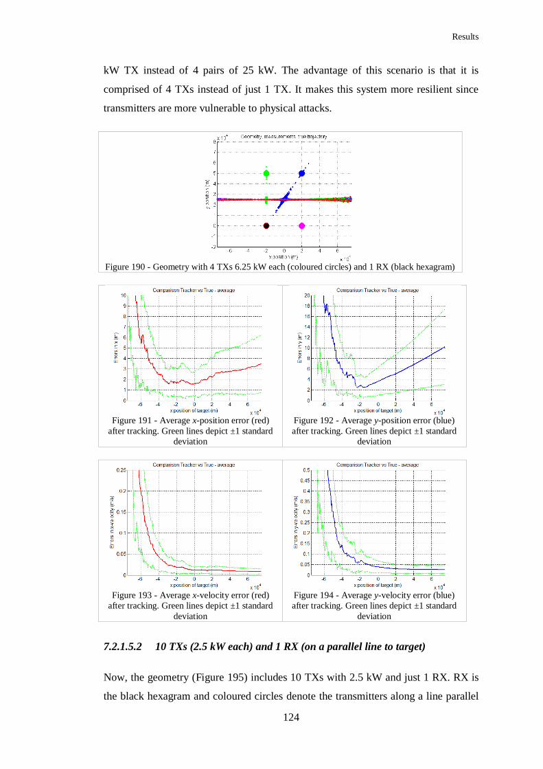
Results
124
kW TX instead of 4 pairs of 25 kW. The advantage of this scenario is that it is
comprised of 4 TXs instead of just 1 TX. It makes this system more resilient since
transmitters are more vulnerable to physical attacks.
Figure 190 - Geometry with 4 TXs 6.25 kW each (coloured circles) and 1 RX (black hexagram)
Figure 191 - Average x-position error (red)
after tracking. Green lines depict ±1 standard
deviation
Figure 192 - Average y-position error (blue)
after tracking. Green lines depict ±1 standard
deviation
Figure 193 - Average x-velocity error (red)
after tracking. Green lines depict ±1 standard
deviation
Figure 194 - Average y-velocity error (blue)
after tracking. Green lines depict ±1 standard
deviation
7.2.1.5.2 10 TXs (2.5 kW each) and 1 RX (on a parallel line to target)
Now, the geometry (Figure 195) includes 10 TXs with 2.5 kW and just 1 RX. RX is
the black hexagram and coloured circles denote the transmitters along a line parallel
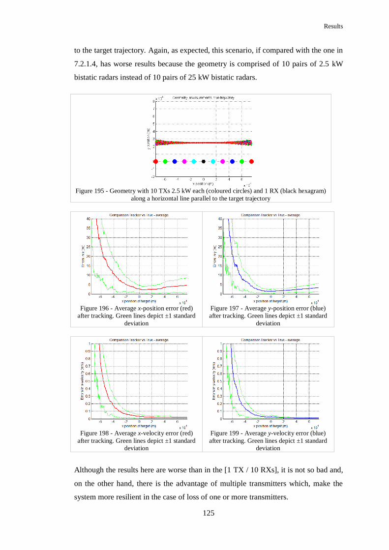
Results
125
to the target trajectory. Again, as expected, this scenario, if compared with the one in
7.2.1.4, has worse results because the geometry is comprised of 10 pairs of 2.5 kW
bistatic radars instead of 10 pairs of 25 kW bistatic radars.
Figure 195 - Geometry with 10 TXs 2.5 kW each (coloured circles) and 1 RX (black hexagram)
along a horizontal line parallel to the target trajectory
Figure 196 - Average x-position error (red)
after tracking. Green lines depict ±1 standard
deviation
Figure 197 - Average y-position error (blue)
after tracking. Green lines depict ±1 standard
deviation
Figure 198 - Average x-velocity error (red)
after tracking. Green lines depict ±1 standard
deviation
Figure 199 - Average y-velocity error (blue)
after tracking. Green lines depict ±1 standard
deviation
Although the results here are worse than in the [1 TX / 10 RXs], it is not so bad and,
on the other hand, there is the advantage of multiple transmitters which, make the
system more resilient in the case of loss of one or more transmitters.

Results
126
7.2.1.6 Multistatic (2 TXs and 2 RXs)
In this scenario, 2 TXs (12.5 kW) and 2 RXs results in 4 pairs of 12.5 kW bistatic
radars. Comparing, this geometry with the previous one [10 TXs and 1 RX], this one
is better and one could choose this geometry instead of the previous one if it were to
reduce deployment costs or to minimize synchronization problems.
Figure 200 - Geometry with 2 TXs 12.5 kW each (blue/green) and 2 RXs (red/magenta) along a
horizontal line parallel to target trajectory
Figure 201 - Average x-position error (red)
after tracking. Green lines depict ±1 standard
deviation
Figure 202 - Average y-position error (blue)
after tracking. Green lines depict ±1 standard
deviation
Figure 203 - Average x-velocity error (red)
after tracking. Green lines depict ±1 standard
deviation
Figure 204 - Average y-velocity error (blue)
after tracking. Green lines depict ±1 standard
deviation

Results
127
This scenario, if compared with the [1 TX and 10 RXs] geometry is worse, but
instead has one more transmitter which might be good depending on how the radar is
intended to be used.
7.2.2 Target 2 (spiral-like trajectory)
In the following scenarios, the target starts at about (-76,0) km and flies on a spiral
trajectory towards one transmitter of the network during 1000 seconds. In this
section, in all the figures except the one that shows the geometry, the x-axis
represents the measurement sequence number. For each scenario, 100 simulation
runs are performed in order to calculate the average and standard deviation of the
results.
In a spiral trajectory, the target changes direction in either x-axis or y-axis a couple of
times. In all scenarios in this section, the first change of direction occurs at around
measurement number 110 where vy is zero and the target is at the top of the spiral.
The next change of direction occurs at around measurement number 230 where vx is
zero and the target is on the right of the spiral. The last change of direction of this
trajectory occurs at around measurement number 330, where vy is zero and the target
is at the bottom of the spiral, very close to the aimed transmitter. The simulation
finishes at measurement number 400, thus 70 measurements after the last change of
direction and it means 175 seconds later. The trajectory finishes 5 km far from the
transmitter at position (0,-5) km.
7.2.2.1 Monostatic
As can be seen in Figure 205 and Figure 206, the velocity and acceleration varies
during the whole trajectory of the target. In both figures, red lines depict the x-axis
true values and blue lines depict the y-axis true values for velocity and acceleration.
Note that the maximum absolute velocity in either axis is about 350 m/s and the
maximum absolute acceleration is about 1.6 m/s2. Figure 207 depicts the target
trajectory and radar location (black circle).

Results
128
Figure 205 – The red (x-velocity) and blue (y-
velocity) depict the true target velocities
Figure 206 - The red (x-acceleration) and blue (y-
acceleration) depict the true target accelerations
Figure 207 – Geometry with one monostatic radar (black circle at (0,0)) and a target with spiral
trajectory
Figure 208 and Figure 209 depict the average position errors in x and y-axis after
tracking.
Figure 208 – Average x-position error (red)
after tracking on each measurement. Green
lines depict ±1 standard deviation
Figure 209 - Average y-position error (blue)
after tracking on each measurement. Green
lines depict ±1 standard deviation
Figure 210 and Figure 211 show the average velocity errors in x and y-axis after
tracking.

Results
129
Figure 210 - Average x-velocity error (red)
after tracking on each measurement. Green
lines depict ±1 standard deviation
Figure 211 - Average y-velocity error (blue)
after tracking on each measurement. Green
lines depict ±1 standard deviation
Figure 212 and Figure 213 present the average acceleration errors in x and y-axis
after tracking.
Figure 212 - Average x-acceleration error (red)
after tracking on each measurement. Green
lines depict ±1 standard deviation
Figure 213 - Average y-acceleration error (blue)
after tracking on each measurement. Green lines
depict ±1 standard deviation
7.2.2.2 Bistatic
This section shows 2 geometries for a bistatic radar: one where the target crosses the
baseline of the radar and another one where it does not cross the baseline.
7.2.2.2.1 Bistatic (crossing baseline)
This scenario represents a bistatic geometry where in Figure 214, the black circle at
(0,0) km is the TX with 25 kW, the black hexagram at (0,60) km is the RX, the red
line is the true trajectory and the green dots are the measurements. Black line depicts
the filtered trajectory. The following figures (Figure 214 to Figure 220) represent the
same type information as in Figure 207 to Figure 213.

Results
130
Figure 214 - Geometry with one bistatic radar (black circle at (0,0) is TX and black hexagram at
(0,60) km is RX) and a target with spiral trajectory (target crossing baseline)
Overall, it can be seen that this configuration is worse than the previous one
(monostatic case), especially the states (position, velocity and acceleration) in y-axis.
In the x-axis, this scenario is better at the beginning of the trajectory but not so good
at the end of it. Note that there are peaks in the tracking results when the target is
crossing the baseline. The inaccuracy is much more evident on y-axis which is the
axis parallel to baseline. It is shown in Figure 93 and Figure 94 that the
measurements are much more inaccurate in the y-axis as well.
Figure 215 - Average x-position error (red)
after tracking on each measurement. Green
lines depict ±1 standard deviation
Figure 216 - Average y-position error (blue)
after tracking on each measurement. Green
lines depict ±1 standard deviation

Results
131
Figure 217 - Average x-velocity error (red)
after tracking on each measurement. Green
lines depict ±1 standard deviation
Figure 218 - Average y-velocity error (blue)
after tracking on each measurement. Green
lines depict ±1 standard deviation
Figure 219 - Average x-acceleration error (red)
after tracking on each measurement. Green
lines depict ±1 standard deviation
Figure 220 - Average y-acceleration error
(blue) after tracking on each measurement.
Green lines depict ±1 standard deviation
7.2.2.2.2 Bistatic (without crossing baseline)
This scenario represents a bistatic geometry where the target does not cross the
baseline (Figure 221). The total power is still 25 kW. Figure 221 to Figure 227
represent the same type of information as in figures in the previous scenario. In this
scenario, the position errors are big when the target is far from the radar, as expected,
in the region between the top of spiral and the right of it. Overall this geometry, if
compared with the monostatic case, is better at the beginning of the trajectory but
worse elsewhere. This is correct, according to the model, since at the beginning of
the trajectory the transmitted signal does not have to travel back to the monostatic
TX/RX because the RX is very close to the beginning of trajectory.

Results
132
Figure 221 - Geometry with one bistatic radar (black circle at (0,0) is TX and black hexagram at
(-60,0) km is RX) and a target with spiral trajectory
Figure 222 - Average x-position error (red)
after tracking on each measurement. Green
lines depict ±1 standard deviation
Figure 223 - Average y-position error (blue)
after tracking on each measurement. Green
lines depict ±1 standard deviation
Figure 224 - Average x-velocity error (red)
after tracking on each measurement. Green
lines depict ±1 standard deviation
Figure 225 - Average y-velocity error (blue)
after tracking on each measurement. Green
lines depict ±1 standard deviation
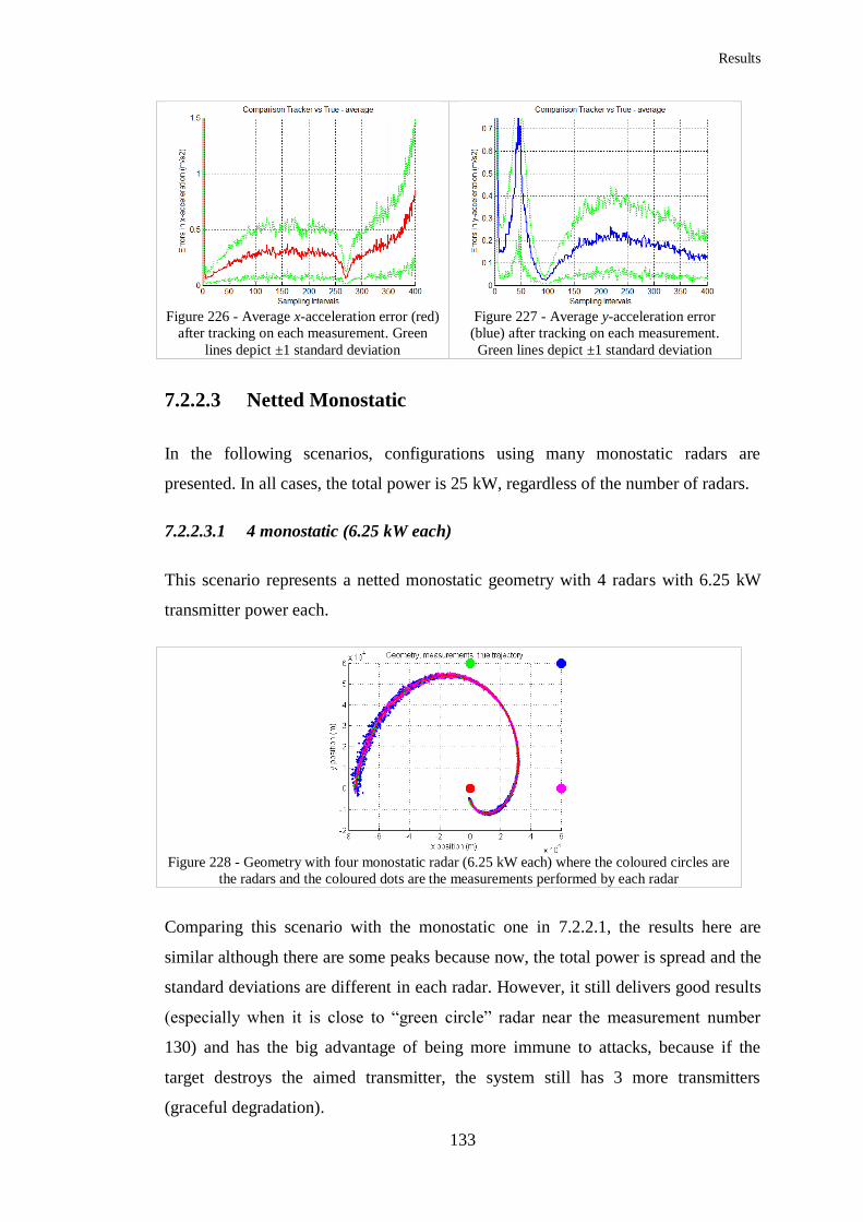
Results
133
Figure 226 - Average x-acceleration error (red)
after tracking on each measurement. Green
lines depict ±1 standard deviation
Figure 227 - Average y-acceleration error
(blue) after tracking on each measurement.
Green lines depict ±1 standard deviation
7.2.2.3 Netted Monostatic
In the following scenarios, configurations using many monostatic radars are
presented. In all cases, the total power is 25 kW, regardless of the number of radars.
7.2.2.3.1 4 monostatic (6.25 kW each)
This scenario represents a netted monostatic geometry with 4 radars with 6.25 kW
transmitter power each.
Figure 228 - Geometry with four monostatic radar (6.25 kW each) where the coloured circles are
the radars and the coloured dots are the measurements performed by each radar
Comparing this scenario with the monostatic one in 7.2.2.1, the results here are
similar although there are some peaks because now, the total power is spread and the
standard deviations are different in each radar. However, it still delivers good results
(especially when it is close to “green circle” radar near the measurement number
130) and has the big advantage of being more immune to attacks, because if the
target destroys the aimed transmitter, the system still has 3 more transmitters
(graceful degradation).

Results
134
Figure 229 - Average x-position error (red)
after tracking on each measurement. Green
lines depict ±1 standard deviation
Figure 230 - Average y-position error (blue)
after tracking on each measurement. Green
lines depict ±1 standard deviation
Figure 231 - Average x-velocity error (red)
after tracking on each measurement. Green
lines depict ±1 standard deviation
Figure 232 - Average y-velocity error (blue)
after tracking on each measurement. Green
lines depict ±1 standard deviation
Figure 233 - Average x-acceleration error (red)
after tracking on each measurement. Green
lines depict ±1 standard deviation
Figure 234 - Average y-acceleration error
(blue) after tracking on each measurement.
Green lines depict ±1 standard deviation
7.2.2.3.2 4 monostatic (6.25 kW each) – closer to the target
This scenario, if compared to the previous one, is undoubtedly better, because the
radars are much closer to the target. In addition, if this geometry is compared with
the monostatic radar with 25 kW in 7.2.2.1, it shows that this geometry has better
results especially during the initial measurements with the position estimates

Results
135
converging faster. The final result, in terms of location is overall better than the
monostatic case. Nevertheless, there are some peaks in the velocity and acceleration
estimates which do not change significantly the position results. Furthermore, this
geometry is still more immune to attacks from enemies and consequently, the system
is more resilient.
Figure 235 - Geometry with four monostatic radar (6.25 kW each) where the coloured circles are the
radars and the coloured dots are the measurements performed by each radar
Figure 236 - Average x-position error (red) after
tracking on each measurement. Green lines depict
±1 standard deviation
Figure 237 - Average y-position error (blue) after
tracking on each measurement. Green lines depict
±1 standard deviation
Figure 238 - Average x-velocity error (red) after
tracking on each measurement. Green lines depict
±1 standard deviation
Figure 239 - Average y-velocity error (blue) after
tracking on each measurement. Green lines depict
±1 standard deviation

Results
136
Figure 240 - Average x-acceleration error (red)
after tracking on each measurement. Green lines
depict ±1 standard deviation
Figure 241 - Average y-acceleration error (blue)
after tracking on each measurement. Green lines
depict ±1 standard deviation
7.2.2.3.3 10 monostatic (2.5 kW) at the same location
This scenario, with 10 monostatic radars at the same location of 7.2.2.1 but with 10
times less power each produces a total power of 25 kW. The main idea of this
scenario is to compare with the scenario where just one monostatic radar is used and
show that the results are basically the same. This confirms that if it is not possible to
increase the power of a transmitter, then it is possible to use many of them to achieve
the desired transmitter power (as shown in 7.2.1.3.2).
Figure 242 - Geometry with 10 monostatic radar (2.5 kW each) at the same location (0,0)

Results
137
Figure 243 - Average x-position error (red)
after tracking on each measurement. Green
lines depict ±1 standard deviation
Figure 244 - Average y-position error (blue)
after tracking on each measurement. Green
lines depict ±1 standard deviation
Figure 245 - Average x-velocity error (red)
after tracking on each measurement. Green
lines depict ±1 standard deviation
Figure 246 - Average y-velocity error (blue)
after tracking on each measurement. Green
lines depict ±1 standard deviation
Figure 247 - Average x-acceleration error (red)
after tracking on each measurement. Green
lines depict ±1 standard deviation
Figure 248 - Average y-acceleration error
(blue) after tracking on each measurement.
Green lines depict ±1 standard deviation
7.2.2.3.4 10 monostatic (2.5 kW) on a line
This scenario also uses a network of monostatic radars but now they are positioned
along a horizontal line following the target trajectory. In the beginning of the
trajectory the radars are close to each other but the distance between them increases
along the horizontal line. The difference here is that this scenario is better than the

Results
138
previous one at the beginning of the trajectory but not in the middle of it. At the end
of trajectory this geometry is just slightly worse than the previous one although in the
previous one it takes advantage of having a very powerful transmitter close to the
target.
Figure 249 - Geometry with 10 monostatic radar (2.5 kW each) on a line – black circles are
TX/RX
Figure 250 - Average x-position error (red)
after tracking on each measurement. Green
lines depict ±1 standard deviation
Figure 251 - Average y-position error (blue)
after tracking on each measurement. Green
lines depict ±1 standard deviation
Figure 252 - Average x-velocity error (red)
after tracking on each measurement. Green
lines depict ±1 standard deviation
Figure 253 - Average y-velocity error (blue)
after tracking on each measurement. Green
lines depict ±1 standard deviation

Results
139
Figure 254 - Average x-acceleration error (red)
after tracking on each measurement. Green
lines depict ±1 standard deviation
Figure 255 - Average y-acceleration error
(blue) after tracking on each measurement.
Green lines depict ±1 standard deviation
7.2.2.4 Multistatic (1 x N)
This section presents 2 different scenarios where a combination of bistatic radars
result in a Multistatic Radar with 1 TX and many RXs.
7.2.2.4.1 1 TX (25 kW) and 4 RXs
This geometry is comprised of 1 TX (25 kW) at (0,0) km (black circle) and 4 RXs
located around the trajectory. This geometry is very similar to the one with 4
monostatic radars and is compared with it. Figure 256 depicts the geometry where all
4 RXs are in the same location as the 4 monostatic radars in 7.2.2.3.2. In fact, one
pair of “bistatic” radar is working as a monostatic one because they are co-located.
Figure 256 - Geometry with 1 TX (black circle) and 4 RXs (coloured hexagrams) and a target
with spiral trajectory
Figure 257 and Figure 258 depict the tracking results and compared with the 4
monostatic case, it shows that this one is better in the beginning of the trajectory for
x-axis. The main point to be noted here, is that in the multistatic case, when the target

Results
140
is getting closer to the end of the trajectory, it crosses 2 bistatic radar baselines what
makes the results to be not so good, although there is a very strong “monostatic” (1
TX and 1 RX collocated) in this region (black/red pair).
Figure 257 - Average x-position error (red)
after tracking on each measurement. Green
lines depict ±1 standard deviation
Figure 258 - Average y-position error (blue)
after tracking on each measurement. Green
lines depict ±1 standard deviation
Therefore, although it was expected that this geometry was better than the four 6.25
kW netted monostatic radar presented in 7.2.2.3.2, this geometry, which comprises 4
pairs of 25 kW bistatic radars, is just slightly better than the netted monostatic one.
Figure 259 - Average x-velocity error (red)
after tracking on each measurement. Green
lines depict ±1 standard deviation
Figure 260 - Average y-velocity error (blue)
after tracking on each measurement. Green
lines depict ±1 standard deviation

Results
141
Figure 261 - Average x-acceleration error (red)
after tracking on each measurement. Green
lines depict ±1 standard deviation
Figure 262 - Average y-acceleration error
(blue) after tracking on each measurement.
Green lines depict ±1 standard deviation
7.2.2.4.2 1 TX (25 kW) and 10 RXs (on a horizontal line)
Here, 10 pairs of 25 kW bistatic radars are put on a horizontal line. TX (25 kW) is
located in the middle of this line of radars with 5 RXs to the left and 5 RXs to the
right. Overall, the results presented here are better than the results in 7.2.2.3.4.
However, it seems that estimates are just similar at the end of trajectory. This might
be due to the fact that the target crosses 4 baselines when it is near (25,0) km.
Figure 263 - Geometry with one TX (black circle) and 10 RXs (coloured hexagrams) along a
horizontal line and a target with spiral trajectory

Results
142
Figure 264 - Average x-position error (red)
after tracking on each measurement. Green
lines depict ±1 standard deviation
Figure 265 - Average y-position error (blue)
after tracking on each measurement. Green
lines depict ±1 standard deviation
Figure 266 - Average x-velocity error (red)
after tracking on each measurement. Green
lines depict ±1 standard deviation
Figure 267 - Average y-velocity error (blue)
after tracking on each measurement. Green
lines depict ±1 standard deviation
Figure 268 - Average x-acceleration error (red)
after tracking on each measurement. Green
lines depict ±1 standard deviation
Figure 269 - Average y-acceleration error
(blue) after tracking on each measurement.
Green lines depict ±1 standard deviation
7.2.2.5 Multistatic (M x 1)
This section presents 2 different scenarios where a combination of bistatic radars
results in a Multistatic Radar with many TXs and 1 RX.
7.2.2.5.1 4 TXs (6.25 kW each) and 1 RX

Results
143
This section presents a geometry with 4 pairs of 6.25 kW bistatic radars. One of
those bistatic radars is actually a monostatic one because TX and RX (red/black pair)
are co-located at (0,0). This geometry is compared with the 1xN multistatic case in
7.2.2.4.1. The geometry presented here has worse results and it can be seen by
comparing Figure 271 and Figure 272 with Figure 257 and Figure 258. It is an
expected result because here 4 pairs of 6.25 kW bistatic radars are used instead of 4
pairs of 25 kW bistatic in 7.2.2.4.1. Nonetheless, it is always worth mentioning that
this geometry could be an option if a more resilient system is desirable.
Figure 270 - Geometry with 4 TXs 6.25 kW each (coloured circles) and 1 RX (black hexagram)
and a target with spiral trajectory
Figure 271 - Average x-position error (red)
after tracking on each measurement. Green
lines depict ±1 standard deviation
Figure 272 - Average y-position error (blue)
after tracking on each measurement. Green
lines depict ±1 standard deviation
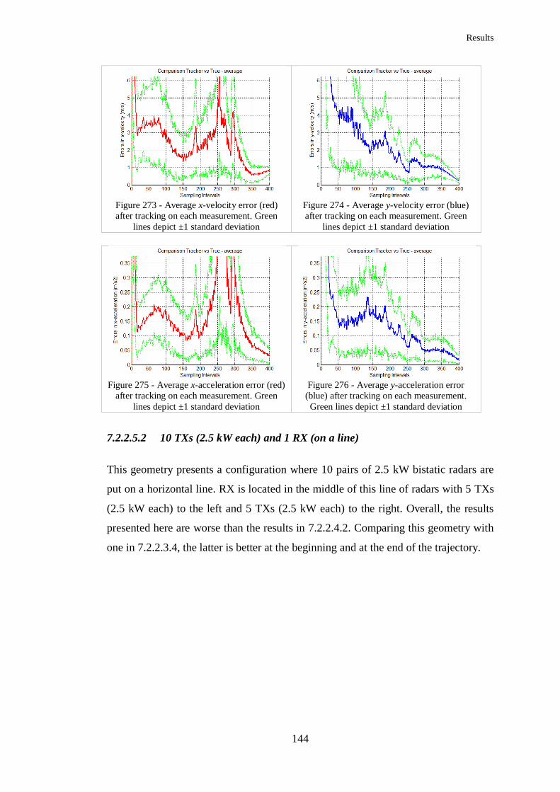
Results
144
Figure 273 - Average x-velocity error (red)
after tracking on each measurement. Green
lines depict ±1 standard deviation
Figure 274 - Average y-velocity error (blue)
after tracking on each measurement. Green
lines depict ±1 standard deviation
Figure 275 - Average x-acceleration error (red)
after tracking on each measurement. Green
lines depict ±1 standard deviation
Figure 276 - Average y-acceleration error
(blue) after tracking on each measurement.
Green lines depict ±1 standard deviation
7.2.2.5.2 10 TXs (2.5 kW each) and 1 RX (on a line)
This geometry presents a configuration where 10 pairs of 2.5 kW bistatic radars are
put on a horizontal line. RX is located in the middle of this line of radars with 5 TXs
(2.5 kW each) to the left and 5 TXs (2.5 kW each) to the right. Overall, the results
presented here are worse than the results in 7.2.2.4.2. Comparing this geometry with
one in 7.2.2.3.4, the latter is better at the beginning and at the end of the trajectory.

Results
145
Figure 277 - Geometry with 10 TXs 2.5 kW each (coloured circles) and one RX (black hexagram)
along a horizontal line and a target with spiral trajectory
Figure 278 - Average x-position error (red) after
tracking on each measurement. Green lines depict
±1 standard deviation
Figure 279 - Average y-position error (blue) after
tracking on each measurement. Green lines depict
±1 standard deviation
Figure 280 - Average x-velocity error (red) after
tracking on each measurement. Green lines depict
±1 standard deviation
Figure 281 - Average y-velocity error (blue) after
tracking on each measurement. Green lines depict
±1 standard deviation

Results
146
Figure 282 - Average x-acceleration error (red)
after tracking on each measurement. Green lines
depict ±1 standard deviation
Figure 283 - Average y-acceleration error (blue)
after tracking on each measurement. Green lines
depict ±1 standard deviation
7.2.2.6 Multistatic (2 TXs and 2 RXs)
In this scenario, there are 2 TXs (12.5 kW) and 2 RXs, comprising 4 pairs of 12.5
kW bistatic radars. Comparing, this geometry with the one [10 TXs and 1 RX], they
are very similar but this scenario is better at the beginning of the trajectory. Besides,
one could decide to implement this one if it were to reduce deployment costs or to
minimize synchronization problems. Note, in Figure 286, that for y-axis position,
there is a peak between measurement 250 and 300 that might be because the target is
crossing the baseline of the bistatic pairs (green-magenta and blue-magenta).
Figure 284 – Geometry with 2 TXs 12.5 kW each (blue/green) and 2 RXs (red/magenta) along a
horizontal line and a target with spiral trajectory

Results
147
Figure 285 - Average x-position error (red)
after tracking on each measurement. Green
lines depict ±1 standard deviation
Figure 286 - Average y-position error (blue)
after tracking on each measurement. Green
lines depict ±1 standard deviation
Figure 287 - Average x-velocity error (red)
after tracking on each measurement. Green
lines depict ±1 standard deviation
Figure 288 - Average y-velocity error (blue)
after tracking on each measurement. Green
lines depict ±1 standard deviation
Figure 289 - Average x-acceleration error (red)
after tracking on each measurement. Green
lines depict ±1 standard deviation
Figure 290 - Average y-acceleration error
(blue) after tracking on each measurement.
Green lines depict ±1 standard deviation
This scenario, if compared with the geometry (1 TX / 10 RXs) in 7.2.2.4.2, is worse.
On the other hand, has one more transmitter which might be good depending on how
the radar is intended to be used.

Results
148
7.2.3 Tracking Summary Tables
7.2.3.1 Target 1
Table 9 summarizes the tracking position errors for x and y-axis for a target that flies
with a constant velocity of 250 m/s and has an RCS of 0.1 m2. All the geometries
presented in 7.2.1 are summarized in this table.
Tables in this section present some quantitative values at certain points of the
trajectory and illustrate the influence of transmitter power and geometry in the
results. However, the graphics in previous sections depict a more thorough idea on
how the tracking accuracy behave along the whole trajectory for different
geometries.
Table 9 – Tracking Results Summary – tracking position errors during the trajectory of a target that
flies on a straight line with constant velocity of 250 m/s
Geometry Tracking Errors for position in x-axis
(m)
Tracking Errors for position in y-axis
(m)
x=-40
km
x=-20
km
x=0 km x=20
km
x=-40
km
x=-20
km
x=0 km x=20 km
(1) Monostatic
(25 kW) 6 2.5 2 2 12 3 0.5 1
(2) Bistatic (25
kW) crossing 0.7 0.5 7.3 0.5 30 15 400 180
(3) Bistatic (25
kW) parallel
TX-RX
18 12 10 7 22 9 2 7
(3a) Bistatic (25
kW) parallel
RX-TX
9 6 10 12 14 8 2 8
(4) Netted
Mono 4 TX/RX (6.25 kW)
4 2 2 1.5 5 1.5 2 1.5
(5) Netted Mono 10
TX/RX (2.5
kW) same
location
6 2.5 2 2 11 3 0.5 1
(6) Netted
Mono 10 TX/RX (2.5
kW) line
2.4 2.4 2 1.9 1.5 1.7 1.9 1.5
(7) Multistatic 1
TX (25 kW)
and 4 RXs
1.8 1.4 1.8 1.7 4 2 1.5 1.5
(8) Multi 1 TX
(25 kW) and 10
RXs line
2 1.6 1 1 2 1 0.8 0.7
(9) Multi 4 TXs (6.25 kW) and 1
RX
2.5 1.8 1.5 2.3 5.8 2.9 3.8 5

Results
149
(10) Multi 10
TXs (2.5 kW) and 1 RX line
11 5 2.5 2.5 7 2.5 2 2.5
(11) Multi 2 TXs (12.5 kW)
and 2 RXs
4.4 4 3.7 3.5 3 2 3 3
Similarly to Table 9, Table 10 depicts the target tracking velocity errors in x and y-
axis at certain x-axis positions.
Table 10 - Tracking Results Summary – tracking velocity errors during the trajectory of a target that
flies on a straight line with constant velocity of 250 m/s
Geometry Tracking Errors for velocity in x-axis
(m/s)
Tracking Errors for velocity in y-axis
(m/s)
x=-40
km
x=-20
km
x=0 km x=20
km
x=-40
km
x=-20
km
x=0 km x=20 km
(1) Monostatic
(25 kW) 0.12 0.05 0.02 0.01 0.25 0.06 0.02 0.01
(2) Bistatic (25
kW) crossing 0.05 0.04 0.5 0.04 2 2 100 38
(3) Bistatic (25
kW) parallel
TX-RX
1.3 1 0.8 0.6 1.5 0.6 0.2 1
(3a) Bistatic (25
kW) parallel
RX-TX
0.7 0.5 0.75 0.9 1 1.2 0.2 0.4
(4) Netted
Mono 4 TX/RX (6.25 kW)
0.06 0.02 0.15 0.1 0.12 0.04 0.02 0.01
(5) Netted Mono 10
TX/RX (2.5
kW) same
location
0.1 0.04 0.02 0.01 0.25 0.06 0.02 0.01
(6) Netted
Mono 10 TX/RX (2.5
kW) line
0.03 0.02 0.015 0.01 0.02 0.015 0.01 0.005
(7) Multistatic 1
TX (25 kW)
and 4 RXs
0.03 0.02 0.015 0.01 0.08 0.03 0.02 0.015
(8) Multi 1 TX
(25 kW) and 10
RXs line
0.03 0.02 0.01 0.01 0.35 0.02 0.01 0.01
(9) Multi 4 TXs
(6.25 kW) and 1 RX
0.045 0.02 0.015 0.015 0.13 0.07 0.04 0.03
(10) Multi 10 TXs (2.5 kW)
and 1 RX line
0.18 0.06 0.04 0.03 0.14 0.05 0.03 0.02
(11) Multi 2
TXs (12.5 kW)
and 2 RXs
0.06 0.03 0.025 0.02 0.05 0.025 0.025 0.02

Results
150
7.2.3.2 Target 2
Target 2 is a target that flies on a spiral-like trajectory with non constant velocity and
acceleration starting from (-100,0) km and going towards one transmitter of the
network. Table 11, Table 12 and
Table 13 depict, respectively the tracking errors for position, velocity and
acceleration for all scenarios from section 7.2.2.
Table 11 - Tracking Results Summary – tracking position errors during the trajectory of a target that
flies on a spiral trajectory with non constant velocity and acceleration. The errors are depicted at
certain measurement sequence number. Each measurement is performed every 2.5 seconds.
Geometry Tracking Errors for position
in x-axis (m)
Tracking Errors for position in
y-axis (m)
At 100 At 200 At 350 At 100 At 200 At 350
(1) Monostatic (25 kW) 45 15 2 25 15 2
(2a) Bistatic (25 kW) crossing 10 2 20 20 30 15
(2b) Bistatic (25 kW) 60 50 20 10 70 20
(3a) Netted Mono 4 TX/RX (6.25 kW)
6 28 3 10 14 2
(3b) Netted Mono 4 TX/RX (6.25 kW) closer
8 3 3 10 4 3
(3c) Netted Mono 10 TX/RX (2.5 kW) same location
43 12 2 20 14 2
(3d) Netted Mono 10 TX/RX (2.5
kW) line 47 12 15 33 15 3
(4a) Multistatic 1 TX (25 kW)
and 4 RXs 15 8 3 10 7 2
(4b) Multistatic 1 TX (25 kW)
and 10 RXs line 23 8 3 15 10 2
(4c) Multistatic 4 TXs (6.25 kW)
and 1 RX 30 13 3 26 14 2
(4d) Multistatic 10 TXs (2.5 kW)
and 1 RX line 45 20 4 20 10 2
(5) Multistatic 2 TXs (12.5 kW)
and 2 RXs 40 16 14 29 18 7
Table 12 - Tracking Results Summary – tracking velocity errors during the trajectory of a target that
flies on a spiral trajectory with non constant velocity and acceleration. The errors are depicted at
certain measurement sequence number. Each measurement is performed every 2.5 seconds.
Geometry Tracking Errors for velocity
in x-axis (m/s)
Tracking Errors for velocity in
y-axis (m/s)
At 100 At 200 At 350 At 100 At 200 At 350
(1) Monostatic (25 kW) 4.8 2.5 0.7 3.7 2.5 0.9
(2a) Bistatic (25 kW) crossing 2.4 1.4 2.5 3 5 3
(2b) Bistatic (25 kW) 6 6 4 2 5 2.8
(3a) Netted Mono 4 TX/RX (6.25
kW) 1 6 0.8 2.2 1.8 1
(3b) Netted Mono 4 TX/RX (6.25
kW) closer 1.3 1.4 0.6 2.4 2.4 1

Results
151
(3c) Netted Mono 10 TX/RX (2.5
kW) same location 3.5 1.6 0.5 2.6 1.8 0.9
(3d) Netted Mono 10 TX/RX (2.5
kW) line 4 1.5 0.5 4.2 3 1
(4a) Multistatic 1 TX (25 kW)
and 4 RXs 2 1.9 0.7 2.2 1.3 0.9
(4b) Multistatic 1 TX (25 kW)
and 10 RXs line 2.2 1.4 0.6 3.1 2.5 1
(4c) Multistatic 4 TXs (6.25 kW)
and 1 RX 3 2.2 0.6 3.5 2 0.9
(4d) Multistatic 10 TXs (2.5 kW)
and 1 RX line 4 2 0.9 2.2 1.6 1
(5) Multistatic 2 TXs (12.5 kW)
and 2 RXs 3.5 2 2 5 3.4 1.8
Table 13 - Tracking Results Summary – tracking acceleration errors during the trajectory of a target
that flies on a spiral trajectory with non constant velocity and acceleration. The errors are depicted at
certain measurement sequence number. Each measurement is performed every 2.5 seconds.
Geometry Tracking Errors for
acceleration in x-axis (m/s2)
Tracking Errors for
acceleration in y-axis (m/s2)
At 100 At 200 At 350 At 100 At 200 At 350
(1) Monostatic (25 kW) 0.23 0.17 0.08 0.18 0.19 0.07
(2a) Bistatic (25 kW) crossing 0.24 0.01 0.17 0.2 0.35 0.35
(2b) Bistatic (25 kW) 0.3 0.3 0.4 0.04 0.22 0.15
(3a) Netted Mono 4 TX/RX (6.25 kW) far
0.1 0.6 0.06 0.1 0.12 0.06
(3b) Netted Mono 4 TX/RX (6.25 kW) closer
0.12 0.05 0.06 0.09 0.1 0.07
(3c) Netted Mono 10 TX/RX (2.5
kW) same location 0.23 0.07 0.04 0.07 0.12 0.04
(3d) Netted Mono 10 TX/RX (2.5
kW) line 0.23 0.05 0.05 0.25 0.25 0.1
(4a) Multistatic 1 TX (25 kW)
and 4 RXs 0.15 0.1 0.08 0.08 0.1 0.07
(4b) Multistatic 1 TX (25 kW)
and 10 RXs line 0.15 0.05 0.07 0.2 0.3 0.08
(4c) Multistatic 4 TXs (6.25 kW)
and 1 RX 0.18 0.11 0.07 0.17 0.13 0.05
(4d) Multistatic 10 TXs (2.5 kW)
and 1 RX line 0.22 0.09 0.07 0.06 0.11 0.03
(5) Multistatic 2 TXs (12.5 kW)
and 2 RXs 0.16 0.1 0.14 0.35 0.3 0.13
7.3 Analysis
Sections 7.1 and 7.2 present the simulations performed in several different scenarios
where some parameters are varied in order to assess how the performance of the
radars are affected in terms of measurements and tracking when compared with the
real state of the target. Section 7.1.5 and 7.2.3 show, respectively for measurement
and tracking, a summary of position errors (measurement and tracking), velocity
errors (tracking) and acceleration errors (tracking) when it is applicable.

Results
152
All the results in Section 7.1 are according to the model that uses the radar range
equation (9). When the RCS is reduced by 20 dB (from 10 m2 to 0.1 m
2), SNR is also
reduced by 20 dB. Moreover, when the transmitter power is reduced by a factor of 4
(or 6 dB), SNR is also reduced by the same factor according to the radar equation. In
scenarios where a multistatic radar is used, comparing a multistatic radar with 1 TX
(25 kW) and 2 RXs against a multistatic radar with 2 TXs (12.5 kW each) and 1 RX,
because of the process of fusion, it is shown that having 2 pairs of 12.5 kW bistatic
radars is not necessarily worse than having 2 pairs of 25 kW bistatic radars. In some
situations, for example, in Table 5, when x=-50 km the fused measurement errors for
x-position are the same (800 m) in both multistatic scenarios. The same happens for
y-position when x=0 km. And, although it is useful to compare the numbers
presented in Table 5, it is easier to see the differences when comparing, for example,
Figure 122 with Figure 133 or Figure 123 with Figure 134.
In section 7.2, several scenarios are presented in order to bring a better understanding
about the benefits of using a multistatic radar when tracking a target, either using a
network of monostatic radars or a set of bistatic radars. Again, although the tables in
section 7.2.3 present quantitatively the errors in a form where it might be easy to
compare different scenarios at once, the tables do not show how the numbers are
changing at a certain time. Sometimes, having a better number at x=0, is worse as
whole because, after that it might be increasing or changing abruptly. For example,
line (2a) of Table 11 indicates that the tracking error for position in y-axis changes
from 20 m at measurement number 100 to 30 m at measurement number 200.
However, it does not show that between measurements number 100 and 200 (see
Figure 216), there is a peak where the errors are very large (more than 150 m).
Nonetheless, it is possible to see, when comparing lines (3b) and (4a) of the same
table that using a netted monostatic radar with 4 radars of 6.25 KW is slightly better
than using 4 pair of 25 KW bistatic radars. This is probably because, in this case, the
target is crossing the baseline of a bistatic pair at a certain point of the trajectory.
Section 7.2.1 and 7.2.2 present the results when a target is flying with a constant
velocity and in a spiral–like trajectory, respectively. In both cases, many different
scenarios are simulated keeping the total transmitted power equal to 25 kW. One
difference between those 2 situations is that the results for

Results
153
position/velocity/acceleration errors are spikier in the “Target 2” scenarios. This is
due to the fact that Kalman Filter has to be set for a situation where it expects a non
constant behaviour of the target.
Either for target 1 (Section 7.2.1) or target 2 (Section 7.2.2), simulations show the
advantages of using a combination of radar measurements to track a target. The idea
of all simulations is to show that it is not easy to track a target with RCS of 0.1 m2,
which is about 100 or even more times worse than the expected target RCS of this
kind of radar with 25 kW power. The radar with 25 kW is a typical radar for
navigation purposes where the main targets are located no more than the horizon
distance (around 25 km for ships, which may have an RCS of tens or even hundreds
and thousands of square meters). For targets, like aircrafts flying at a height of 10
km, the horizon distance can be around 400 km (see Table 2), which is quite far for a
radar like this to detect and track an aircraft with RCS=0.1 m2. For a target with such
RCS flying at a distance of about 65 km, the tracking error for x-position is about 15
m (Figure 145) after some time tracking the target (about 60 seconds). This error can
be as good as 1.5 m if the RCS is increased to 10 m2. Thus, the main challenge is to
obtain better results when tracking 0.1 m2 RCS targets using 25 kW radar built for
navigation purposes.
Sections 7.2.1.3.2 and 7.2.2.3.3 are examples that show that combining 10 radars of
2.5 kW has equivalent results to a radar with 25 kW (or even slightly better). It
means that it is possible to emulate a radar of 250 kW power, for example, just using
10 radars of 25 kW at the same location. Problems with interference or timing are not
considered in this study though.
The results also show that distributing the power of the radar along the trajectory
(compare Figure 171 and Figure 177, for example) makes it to converge quicker to a
certain level of error, but it does not get better along the trajectory.
Scenarios where the target crosses the baseline of a bistatic radar present worse
results with the filter and fusion algorithm being used. It is possible to see as well
(comparing Figure 150 and Figure 151) that tracking results are better along the axis
that crosses the baseline. Figure 150 shows that it has the best x-position track results

Results
154
at the beginning of the track if compared with all the other geometries (see line (2) of
Table 9).
Scenarios with just one TX with 25 kW can have much better results when using
many receivers to make use of this power, making the system as a whole be
comprised of many bistatic radars with 25 kW (Figure 185, for example). This
scenario with the same total power as the monostatic case (Figure 144) is overall
better when comparing the results for tracking position (Figure 145, Figure 186 and
Table 9).
A scenario that keeps that same total power, spreading the power along many TXs,
using only 1 RX is also simulated (Figure 195). In this case, the system comprises 10
TXs with 2.5 kW power and 1 RX. The results are worse than the 1 TX and many
RXs scenario but there is the big advantage of having many TXs which makes the
system more resilient to attacks against the TXs. The system can still work with
some degraded performance when one or more TXs are destroyed, for example.
The same ideas of changing the geometry of a radar are applied with target 2. Figure
205 and Figure 206 show how velocity and acceleration of the target are varying
according to time in a spiral-like trajectory (Figure 207).
In section 7.2.2 there are scenarios that show that there is a good improvement on the
results when the radars are brought closer to the target for monostatic cases (Figure
228 and Figure 235), which is an expected result. Nevertheless, the use of 4 bistatic
radars (25 kW pairs) like in Figure 256, instead of 4 monostatic 6.25 kW radars
(Figure 235), does not show better results. In fact, the results are very similar, but in
the first moment, it is not an expected result. The fact that the target crosses the
baseline of 2 of those 4 bistatic radars, can make the system have more modest
results. At the beginning of the trajectory, though, the multistatic radar performs
better (comparing Figure 236 and Figure 257).
Overall, the tracking and fusion algorithm performed well and according to expected.
However, there are cases where, especially for acceleration and velocity, the filter
presents some peaks during the estimation of these states (see, for example Figure
232, Figure 234, Figure 237, Figure 239, Figure 240, Figure 260, Figure 261, Figure
262 and so on). The good thing is that, apparently, the position tracking results are

Results
155
not affected. The existence of peaks seems to be related to the fusion process and
how information about output from the fusion is passed to Kalman Filter.
7.4 Examples
To summarize and to illustrate what can be done with the information from the
previous sections, this section shows the same scenario as in 7.2.2.4.1. The target
flies in a spiral-like trajectory and has RCS=0.1 m2. The main objective in this
example is to improve the tracking results especially at the beginning of the
trajectory (script31.m is used).
The comparison is done against Figure 257 and Figure 258.
Figure 291 depicts the same geometry but instead of using one TX of 25 kW, 10 TXs
of 25 kW are used. The results are depicted in Figure 292 and Figure 293. As the
total power increases by a factor of 10, SNR also increases by the same amount. And
the errors, consequently (according to Equations (18) and (19)), decrease by a factor
of . If it was possible to use just one TX of 250 kW, the results would be very
similar.
Figure 291 - Geometry with 10 TXs (black circle) at (0,0) and 4 RXs (coloured hexagrams) and a
target with spiral trajectory

Results
156
Figure 292 - Average x-position error (red) after
tracking on each measurement. Green lines depict
±1 standard deviation
Figure 293 - Average y-position error (blue) after
tracking on each measurement. Green lines depict
±1 standard deviation
Despite the fact that overall the errors are better, at the beginning of the trajectory, it
is still not so good. Next scenario, with the same 10 TXs of 25 kW but with 3 of 4
RXs repositioned, it is possible to improve this requirement. This improvement
comes by changing the position of an RX (green hexagram) to somewhere closer to
the beginning of trajectory and to reposition other 2 RXs (blue and magenta
hexagrams) to a place where the target would not cross the baseline of pairs of
bistatic radars (see Figure 294).
Figure 294 - Geometry with 10 TXs (black circle) at (0,0) and 4 RXs (coloured hexagrams) and a
target with spiral trajectory

Results
157
Figure 295 - Average x-position error (red) after
tracking on each measurement. Green lines depict
±1 standard deviation
Figure 296 - Average y-position error (blue) after
tracking on each measurement. Green lines depict
±1 standard deviation
Figure 295 and Figure 296 depict the results of tracking position errors using the new
geometry and, as expected, the tracking position errors are much better now. A great
improvement happened especially in y-axis position accuracy as can be seen
comparing Figure 296 with Figure 293.
Now, for the same scenario shown in Figure 294 but with just one TX of 250 kW
(for simplicity) and 4 RXs, the measurements of the 4 bistatic pairs are not
performed at the same time. Instead, they are alternated and there is one
measurement done by one of the 4 bistatic pairs every 0.625 seconds (
seconds).
As can be seen in Figure 297 and Figure 298, the average position errors have the
similar magnitude although in this last scenario the errors are spikier. This is due to
the fact that each pair of bistatic radar has different measurement standard deviations
which affect the output of Kalman Filter.
Figure 297 - Average x-position error (red) after
tracking on each measurement. Green lines depict
±1 standard deviation
Figure 298 - Average y-position error (blue) after
tracking on each measurement. Green lines depict
±1 standard deviation

Results
158
Figure 299 and Figure 300 show, for the same scenario above, how is the behaviour
of the errors if all 4 bistatic pairs perform the measurement at the same time every
2.5 seconds. Again, for simplicity, it is used just one TX of 250 kW and the results
are quite similar to Figure 295 and Figure 296 (where 10 TXs of 25 kW is used).
Figure 299 Average x-position error (red) after
tracking on each measurement. Green lines depict
±1 standard deviation
Figure 300 - Average y-position error (blue) after
tracking on each measurement. Green lines depict
±1 standard deviation
As the last example, Figure 301 represents a scenario where there is only 1 TX (250
kW for simplicity, instead of 10 TXs of 25 kW) and only 1 RX that moves along the
green line trajectory (clockwise direction).
Figure 301 - Geometry with 1 TX (black circle) at (0,0) and 1 RX (red hexagrams) that moves along
the green line (clockwise) and a target with spiral trajectory (red line)
This shows what would happen if a intelligent radar decide to move one RX (or TX)
following the target at a certain distance and keeping the bistatic angle at values that
are smaller than 145-180 degrees.

Results
159
Figure 302 - Average x-position error (red) after
tracking on each measurement. Green lines depict
±1 standard deviation
Figure 303 - Average y-position error (blue) after
tracking on each measurement. Green lines depict
±1 standard deviation
So, with just one RX it is possible to achieve results (see Figure 302 and Figure 303)
that are similar to what is obtained in the previous scenario. To perform this specific
scenario (case 4 of script31.m), another version of class TRadar has to be used and
TRadar1.m must substitute TRadar.m to perform this simulation.

Conclusions and Further Work
160
8 Conclusions and Further Work
The first radars used in military scenarios to detect enemies were quasi-bistatic, due
to the fact that by that time, it had not been developed a technology that would allow
the transmitter and receiver to use the same antenna. After the development of
monostatic radars, there was almost no interest in the bistatic radars subject.
Apparently, this interest in bistatic and multistatic radars has been happening in
cycles of 15-20 years according to [3]. However, due to the fact that monostatic
radars alone have been reaching their limits in terms of performance and because of
the existence of new threats, the interest in bistatic and multistatic radars, nowadays,
should last longer.
In order to detect stealth targets and to be able to overcome jamming attacks by
enemies, networks of radars operating either monostatically or bi/multistatically can
be used. Among many things, this delivers better sensitivity, coverage and tracking
accuracy.
The research reported in this thesis has investigated how much multistatic radars can
be better than stand alone monostatic radars when tracking a target. Simulations with
different geometries and different target trajectories have been performed in order to
assess the tracking performance in each scenario. Although three simple tracking
filters (g-h, g-h-k and KF) have been programmed, only the KF has been used for the
final results. Tracking performance has been analysed in terms of estimated position,
velocity and acceleration accuracies. Different geometries including monostatic
radar, bistatic radars with target crossing and not crossing the baseline, multistatic

Conclusions and Further Work
161
radars with only 1 TX and many RXs, multistatic radars with many TXs and only 1
RX and multistatic radars with many TXs and RXs have been considered.
In terms of target state (position, velocity and acceleration) accuracy of the
measurements and tracking, the simulations have shown that performance is
proportional to the total power of the network transmitters. Nonetheless, depending
on the configuration of the geometry, the results have not been as good as expected.
It happened because the fusion algorithm is very simple and it considers the
measurements from each radar of the network using weights to perform average of
the measurements. While the weight is related to SNR, the algorithm considers
measurements with higher SNR more important than the ones with lower SNR. In
scenarios where the target crosses the baseline of a pair of bistatic radar, it has been
assumed that measurements coming from the region where the bistatic angle is close
to 180 degrees are not very reliable and thus their weights are reduced.
The simulations were performed with real radar characteristics because the idea was
to assess if it was possible to use characteristics of navigation radars to track targets
with low RCS. The research reported in this thesis has shown that it is possible to
achieve a good accuracy configuring a geometry that is suitable for the requirements
of a system.
Also, from the results of the simulations it is possible to understand why multistatic
radars can still work with acceptable accuracy if one TX is lost or destroyed
(graceful degradation). Losing one TX from a multistatic radar with 10 TXs, means
that the total power of the system is reduced to 90% if all TXs are identical. If all
TXs are located at the same position, the reduction in SNR would be the same as the
reduction in total power. Thus, the errors increase by a factor of about 5%.
The problem of jamming attacks to TX does not affect performance of bistatic radars
or multistatic radars comprised of pairs of bistatic radars. In addition, jamming
attacks to a monostatic radar of a network makes the system to perform with a
degraded performance and not to be completely out of service. Besides, an intelligent
system could order the monostatic radar to stop emitting and become just a receiver
in the network making jamming attacks less effective.

Conclusions and Further Work
162
This work has presented several figures that show the tracking accuracy (for position,
velocity and acceleration) of different geometries when the target is flying at certain
velocity and at a certain distance from the radar. Therefore, it is possible to see how
the performance of a tracker can be improved just adding another TX or RX or just
deploying them into a more suitable location. Furthermore, it has shown that if the
technology does not allow the system to have more powerful radars, so adding some
more TXs to the network can help to improve accuracy, for example. Also, if the
budget does not allow buying so many TXs, adding cheap RXs can still enhance the
performance of the system.
Consequently, using more than one monostatic radar, a number of TXs and RXs and
combining information from all radars of a network will allow the system to be more
accurate, more resilient and maybe cheaper. However, there are some improvements
that should be tackled in future research. The report herein presented has considered
that the radars (nodes) of the network communicate without delays or any other
problems related to communication among them. The information necessary for data
fusion is 100% available for the fusion algorithms and then for the tracking
algorithm. Additionally, position estimates have been considered to be known by all
the nodes so that they can point their antennas to the correct region of the space. It is
also considered to be performed by another software module not developed in this
thesis. As a consequence, resource management software should be developed in
order to make the best use of all information that herein is considered available for
all algorithms whenever necessary. Another important characteristic of the
simulations performed in this thesis is that all the measurements have been
performed in fixed intervals of 2.5 seconds. These intervals could be variable
according to the needs of the system if the system uses Electronically Steered
Antennas. Again, “needs of the system” means that there is some module managing
where the resources are most necessary at a certain moment. The same ideas applied
for Multifunctional Radar could be applied on a radar network when it is about
managing the resources of a system [22][36].
This thesis has shown that deploying a radar platform (TX and/or RX) in different
locations can bring better or worse results. A resource management software can also
designate a platform to move during the tracking process to a more suitable location

Conclusions and Further Work
163
according to the needs of the scenario. It would be done especially, for example,
when the system is prepared to launch a missile against a target and more accuracy is
needed. Even the missile can be working cooperatively with some RXs nodes in
order to keep track of the target during its flight even if the target is trying to jam its
TX.
Also, this work has shown quantitatively that the use of navigation radars of 25 kW
(aimed to track ships with RCS of tens, hundreds or thousands of square meters) and
operational frequency of 9.41 GHz (X-band) working co-operatively in a network of
radars makes it possible to track targets with RCS as small as 0.1 m2 flying within
the surveillance area. Uncountable scenarios are possible. This thesis has focused on
working with the same fusion and tracking algorithm and also the basic
characteristics of the radar (operational frequency, PRF, beam width, pulse width,
etc) and only varying the geometry of the radar network to assess its performance.
Some future work may include more simulations changing some other variables such
as pulse width to improve range resolution, measurement accuracy and tracking
accuracy.
Also, from the results of the simulations it is possible to see that bistatic radars have
very good performance along the axis that is crossing its baseline but not so good on
the other axis. Nevertheless, this affirmative is true only when the bistatic angle is
smaller than 145 degrees. This information is very useful, especially if TXs and RXs
can move dynamically while tracking targets in order to have the best precision most
of the time. And, although for bistatic angles around 180 degrees the accuracy of
measurements and tracking are very bad, detection in this region is very high because
of the effect shown in 3.3.4.1 and Figure 16. The information that a target is lying on
the baseline of a bistatic radar might be important especially if another pair of
bistatic radar can be used in order to find the location of the target.
Comparing the results reported in this research with the work present in [55], it
seems that the latter is also a work that shows how tracking accuracy varies in
different scenarios of systems of sensors. Its approach is more spatially oriented
showing how the accuracy varies in the surveillance area. It uses the same idea of
fixing the algorithm and assessing it against different geometries. Nonetheless, it
does not show examples using bistatic radars or even a multistatic radars. Only
Conclusions and Further Work
164
monostatic radars are considered. The work presented in this thesis has a different
approach when presenting the results, showing for a particular target dynamics how
the tracking performance varies when different geometries are used to track the
target. Moreover, the work presented herein has considered that standard deviation in
range and angle vary according to SNR and thus, distance to the target.
In [57], the authors present simulations where the configuration of the radar network
does not change and 4 different target trajectories and 3 different tracking algorithms
are assessed. The paper shows different figures to illustrate the tracking accuracy in
these different situations. Once more, it is another paper that approaches the problem
of tracking a target in a multistatic scenario but it does not include information about
how different configurations of radars would affect the results in tracking accuracy.
On the other hand, important information can be extracted from the paper, for
instance, the difference in tracking accuracy for each tracking algorithm that is
executed.
Some simulations are also performed in the work presented in [24]. In this case, only
measurement accuracy is considered and 5 different configurations of radars are
assessed by the use of “constant accuracy contours”: monostatic case, bistatic case,
netted monostatic, netted bistatic (linear) and netted bistatic (triangular). Similarly to
what has been done in this thesis, the total power of the systems are kept the same to
make the comparisons fairer. [24] though does not go further to investigate tracking
accuracy or to assess some additional geometries with more TXs, for example. From
the same author, [7] presents a multistatic tracking system and makes comparisons
between multistatic and netted monostatic radar systems from the tracking point of
view. Contrasting these two papers [7] [24] with the work herein presented it is
possible to see that this thesis, although not using the same type of graphs, goes
further in the investigation of tracking performance in several different geometries of
multistatic radars usually with more than 2 TXs or RXs.
Additionally, the Matlab code developed for the purpose of this thesis can be reused
and straightforwardly some parameters can be changed in order to assess how
performance changes. Some of the parameters than can be changed include:
transmitter power, beamwidth, operating frequency, pulse width and sampling
interval.

Conclusions and Further Work
165
Further research can be done simulating the use of Electronically Steered Antennas,
assessing scenarios with more than one target, making the platforms to move
intelligently according to the scenario, using 3D geometries and making the radars to
communicate among them in order to synchronize and exchange data. Parameters
that are considered to be ideal by this research can be modelled in further studies, for
example, clutter levels, probability of detection, probability of false alarm data link
delays and missed and out-of-sequence measurements. In addition, improvements in
the algorithms of fusion and tracking can be developed aiming better accuracy and
reduction in the computational load according to each geometry.
Performing simulations with Electronically Steered Antennas will show, for
example, how changing the sampling interval can improve tracking accuracy. The
use of this kind of antenna allows the system to “look” at a certain region of the
space immediately without having to wait for a complete revolution of a rotating
antenna. The agility provided by this kind of antenna allows a resource management
system to make the best use of the existing resources and from the ideas herein
presented, the developer team of such system has an idea of where to move a
platform, where to point the antenna, which sampling interval to use, how much time
to be looking at a certain target and so on.
In addition, from the ideas presented in this thesis, more analysis can be done if more
variables are considered. For example, considering communication links delays can
affect tracking accuracy and thus delays should be quantified and demonstrated how
they could affect the performance of the whole tracking system.
If the resource management system can move the nodes, it is important that the new
positions are accurate. The simulations performed in this thesis have considered that
the location of the platforms were very accurate without errors. Moving the platforms
must be very important if the system is trying to avoid, for example, that a target lies
in the region of the baseline of a bistatic radar. Or even if it is impossible, it can
move some plataforms in order to keep the target on the forward scatter region
(where the detection is very high) of 2 or more bistatic radars in order to find the
position of the target by using high detection information coming from a number of
bistatic radars. The problem here is that it might be necessary to have platforms that
can move at velocities similar to the target velocity.

Conclusions and Further Work
166
Finally, from the work presented in this thesis, it is expected that more aspects of the
scenarios can be taken into account as well as more characteristics of the radar can be
varied in order to help in the development of intelligent and adaptive systems that
will be able to make the best use of all resources of a radar network in order to keep
track of one or more targets.
8.1 Summary
Summarizing, the main contribution of this thesis is to show that it is possible to use
characteristics of simple and cheap navigation radars (when they are used in a
multistatic configuration) to track targets located as far as 70-80 km with RCS (0.1
m2) that is smaller than the RCS of targets that usually this kind of radar is designed
for. In addition, the thesis has shown how several different geometries (with one or
more TXs and RXs) can affect the results in tracking accuracy and also showed
quantitatively the respective accuracies along trajectory of the target.
Some of the most important conclusions include:
- Using the algorithms chosen, it was better to avoid targets crossing the
baseline of bistatic radars
- Adding more TXs to the system made it possible to achieve similar results if
comparing to an equivalent more powerful radar
- Splitting the power of one radar into smaller radars brought similar results
and depending on the geometry could also bring better results, for example,
making the tracking prediction to converge faster
- Geometry is important and being able to move nodes to better locations
according to the needs of the system could bring better results
- Intelligent systems are needed in order to control the network aiming for a
dynamic geometry that changes according to scenario

167
References
[1] J. I. Glaser, „Fifty years of bistatic and multistatic radar‟, IEE Proceedings F -
Communications, Radar and Signal Processing, vol. 133, no. 7, pp. 596–603,
1986.
[2] S. S. Swords, Technical History of the Beginnings of Radar, illustrated ed.
Institution of Engineering and Technology, 1986.
[3] N. J. Willis, Bistatic Radar, 2nd Revised ed. SciTech Publishing Inc, 2005.
[4] G. W. Ng and K. H. Ng, „Sensor management-what, why and how‟,
Information Fusion, vol. 1, no. 2, pp. 67–75, 2000.
[5] H. Durrant-Whyte, „A Beginner‟s Guide to Decentralised Data Fusion‟,
Technical Document of Australian Centre for Field Robotics, University of
Sydney, Australia, 2000.
[6] A. Farina and S. Pardini, „Multiradar Tracking System Using Radial Velocity
Measurements‟, IEEE Transactions on Aerospace and Electronic Systems, vol.
AES-15, no. 4, pp. 555 –563, Jul. 1979.
[7] A. Farina, „Multistatic Tracking and Comparison with Netted Monostatic
Systems‟, Proceedings of the International Conference Radar-82, London, UK,
pp. 183–187, 1982.
[8] A. Farina, „Tracking function in bistatic and multistatic radar systems‟, IEE
Proceedings F - Communications, Radar and Signal Processing,, vol. 133, no.
7, pp. 630–637, 1986.
[9] H. F. Durrant-Whyte, B. Y. . Rao, and H. Hu, „Toward a fully decentralized
architecture for multi-sensor data fusion‟, in IEEE International Conference on
Robotics and Automation, Cincinnati, OH, USA, 1990, vol. 2, pp. 1331 –1336
vol.2.
[10] B. S. Rao and H. F. Durrant-Whyte, „Fully decentralised algorithm for
multisensor Kalman filtering‟, IEE Proceedings D - Control Theory and
Applications, vol. 138, no. 5, pp. 413 –420, Sep. 1991.
[11] M. N. Petsios, E. G. Alivizatos, and N. K. Uzunoglu, „Manoeuvring target
tracking using multiple bistatic range and range-rate measurements‟, Signal
Processing, vol. 87, no. 4, pp. 665–686, 2006.

168
[12] A. D. Lallo, A. Farina, R. Fulconi, A. Stile, L. Timmoneri, and D. Vigilante,
„A Real Time Test Bed for 2D and 3D Multi-Radar Tracking and Data Fusion
with Application to Border Control‟, in CIE ’06. International Conference on
Radar, Shanghai, China, 2006, pp. 1–6.
[13] „IEEE Standard Radar Definitions‟. IEEE Standards, 2008.
[14] H. D. Griffiths, „Bistatic Radar - Principles And Practice‟, in SBMO
International Microwave Conference/Brazil, Sao Paulo, Brazil, 1993, vol. 2, pp.
519–526.
[15] H. D. Griffiths, „From a different perspective: principles, practice and potential
of bistatic radar‟, in International Radar Conference, Adelaide, SA, Australia,
2003, pp. 1–7.
[16] M. I. Skolnik, Radar Handbook, Third Edition, 3rd ed. McGraw-Hill
Professional, 2008.
[17] K. M. Siegel, H. A. Alperin, R. R. Bonkowski, J. W. Crispin, A. L. Maffett, C.
E. Schensted, and I. V. Schensted, „Bistatic Radar Cross Sections of Surfaces of
Revolution‟, Journal of Applied Physics, vol. 26, no. 3, pp. 297 –305, Mar.
1955.
[18] H. Griffiths, „Multistatic, MIMO and networked radar: The future of radar
sensors?‟, in European Radar Conference (EuRAD), Paris, France, 2010, pp. 81
–84.
[19] C. J. Baker, „An Introduction to Multistatic Radar‟, NATO/OTAN, RTO-EN-
SET-133, 2009.
[20] R. E. Kalman, „A new approach to linear filtering and prediction problems‟,
Journal of basic Engineering, vol. 82, no. 1, pp. 35–45, 1960.
[21] G. van Keuk and S. S. Blackman, „On phased-array radar tracking and
parameter control‟, IEEE Transactions on Aerospace and Electronic Systems,
vol. 29, no. 1, pp. 186–194, 1993.
[22] S. Miranda, C. Baker, K. Woodbridge, and H. Griffiths, „Knowledge-based
resource management for multifunction radar: a look at scheduling and task
prioritization‟, IEEE Signal Processing Magazine, vol. 23, no. 1, pp. 66–76,
2006.
[23] S. Haykin, „Cognitive radar: a way of the future‟, IEEE Signal Processing
Magazine, vol. 23, no. 1, pp. 30–40, 2006.
[24] A. Farina and E. Hanle, „Position Accuracy in Netted Monostatic and Bistatic
Radar‟, IEEE Transactions on Aerospace and Electronic Systems, vol. AES-19,
no. 4, pp. 513–520, 1983.
[25] C. J. Baker and A. L. Hume, „Netted radar sensing‟, IEEE Aerospace and
Electronic Systems Magazine, vol. 18, no. 2, pp. 3–6, 2003.
[26] C. J. Baker and H. D. Griffiths, „Bistatic and Multistatic Radar Sensors for
Homeland Security‟, Advances in sensing with security applications, 2006 -
Springer, pp. 1–22, 2006.
[27] H. Griffiths, „Future radar developments‟, Electronics & Communication
Engineering Journal, vol. 14, no. 6, pp. 250–251, 2002.

169
[28] H. D. Griffiths, „New directions in bistatic radar‟, in RADAR ’08. IEEE Radar
Conference, Rome, Italy, 2008, pp. 1–6.
[29] T. Derham, K. Woodbridge, H. Griffiths, and C. J. Baker, „The design and
development of an experimental netted radar system‟, in International Radar
Conference, Adelaide, SA, Australia, 2003, pp. 293–298.
[30] S. Doughty, K. Woodbridge, and C. Baker, „Characterisation of a Multistatic
Radar System‟, in EuRAD 2006. 3rd European Radar Conference, Manchester,
UK, 2006, pp. 5–8.
[31] I. Papoutsis, C. J. Baker, and H. D. Griffiths, „Netted radar and the ambiguity
function‟, in IEEE International Radar Conference, Arlington, VA, USA, 2005,
pp. 883–888.
[32] Y. Teng, S. Doughty, K. Woodbridge, H. Griffiths, and C. Baker, „Netted
Radar Theory and Experiments‟, in IDC ’07. Information, Decision and
Control, Adelaide, SA, Australia, 2007, pp. 23–28.
[33] Y. Teng, H. D. Griffiths, C. J. Baker, and K. Woodbridge, „Netted radar
sensitivity and ambiguity‟, IET Radar, Sonar & Navigation, vol. 1, no. 6, pp.
479–486, 2007.
[34] P. F. Sammartino, C. J. Baker, and M. Rangaswamy, „Moving target
localization with multistatic radar systems‟, in RADAR ’08. IEEE Radar
Conference, Rome, Italy, 2008, pp. 1–6.
[35] A. Farina, P. Lombardo, and M. Marsella, „Joint tracking and identification
algorithms for multisensor data‟, IEE Proceedings - Radar, Sonar and
Navigation, vol. 149, no. 6, pp. 271–280, 2002.
[36] G. T. Capraro, A. Farina, H. Griffiths, and M. C. Wicks, „Knowledge-based
radar signal and data processing: a tutorial review‟, IEEE Signal Processing
Magazine, vol. 23, no. 1, pp. 18–29, 2006.
[37] P. F. Sammartino, C. J. Baker, H. D. Griffiths, and M. Rangaswamy,
„Decentralized processing in radar networks‟, in IET International Conference
on Radar Systems, Edinburgh, UK, 2007, pp. 1–5.
[38] E. G. Alivizatos, M. N. Petsios, and N. K. Uzunoglu, „Architecture of a
multistatic FMCW direction-finding radar‟, Aerospace Science and Technology,
vol. 12, no. 2, pp. 169–176, 2007.
[39] P. F. Sammartino, C. J. Baker, and M. Rangaswamy, „Coverage in radar
networks‟, in ACSSC 2007. Conference Record of the Forty-First Asilomar
Conference on Signals, Systems and Computers, Pacific Grove, California,
USA, 2007, pp. 197–201.
[40] A. P. Hopf, E. J. Knapp, and D. J. McLaughlin, „Scalable Multifunction Dense
Radar Network‟, in IGARSS 2008. IEEE International Geoscience and Remote
Sensing Symposium, Boston, Massachussets, USA, 2008, vol. 4, p. IV – 1018–
IV – 1021.
[41] B. Philips, D. Westbrook, D. Pepyne, J. Brotzge, E. J. Bass, and D. Rude,
„User Evaluations of Adaptive Scanning Patterns in the CASA Spring
Experiment 2007‟, in IGARSS 2008. IEEE International Geoscience and
Remote Sensing Symposium, Boston, Massachussets, USA, 2008, vol. 5, p. V –
156–V – 159.

170
[42] F. Junyent and V. Chandrasekar, „Radar network characterization‟, in IGARSS
2007. IEEE International Geoscience and Remote Sensing Symposium,
Barcelona, Spain, 2007, pp. 2730–2733.
[43] M. Zink, E. Lyons, D. Westbrook, D. Pepyne, B. Pilips, J. Kurose, and V.
Chandrasekar, „Meteorological Command & Control: Architecture and
Performance Evaluation‟, in IGARSS 2008. IEEE International Geoscience and
Remote Sensing Symposium, Boston, Massachussets, USA, 2008, vol. 5, p. V –
152–V – 155.
[44] F. Junyent and V. Chandrasekar, „Weather Radar Network Design‟, in IGARSS
2008. IEEE International Geoscience and Remote Sensing Symposium, Boston,
Massachussets, USA, 2008, vol. 4, p. IV – 1022–IV – 1025.
[45] V. Chandrasekar, D. McLaughlin, J. Brotzge, M. Zink, B. Philips, and Y.
Wang, „Evaluation of Distributed Collaborative Adaptive Sensing in a Four-
Node Radar Network: Integrated Project 1‟, in IGARSS 2008. IEEE
International Geoscience and Remote Sensing Symposium, Boston,
Massachussets, USA, 2008, vol. 5, p. V – 148–V – 151.
[46] D. McLaughlin, E. Knapp, Y. Wang, and V. Chandrasekar, „Distributed
weather radar using X-band active arrays‟, IEEE Aerospace and Electronic
Systems Magazine, vol. 24, no. 7, pp. 21–26, 2009.
[47] J. L. Salazar, A. Hopf, R. F. Contreras, B. Philips, E. J. Knapp, D. McLaughlin,
J. Brotzge, and K. Brewster, „Coverage comparison of short range radar
networks vs. conventional weather radars: Case study in the northwestern
United States‟, in IGARSS 2009. IEEE International Geoscience and Remote
Sensing Symposium, Cape Town, South Africa, 2009, vol. 2, p. II–964–II–967.
[48] D. Pepyne, D. McLaughlin, D. Westbrook, E. Lyons, E. Knapp, S. Frasier, and
M. Zink, „Dense radar networks for low-flyer surveillance‟, in IEEE
International Conference on Technologies for Homeland Security (HST),
Waltham, MA, USA, 2011, pp. 413–418.
[49] „Engineering Research Center for Collaborative Adaptive Sensing of the
Atmosphere (CASA)‟, Engineering Research Center for Collaborative
Adaptive Sensing of the Atmosphere (CASA). [Online]. Available:
http://www.casa.umass.edu. [Accessed: 16-May-2011].
[50] E. Brookner, Tracking and Kalman Filtering Made Easy. Wiley-Interscience,
1998.
[51] H. W. Thomas, G. Maignan, and J. T. Storey, „Tracking in a multiradar
environment‟, Proceedings of the Institution of Electrical Engineers, vol. 123,
no. 3, pp. 191 –194, Mar. 1976.
[52] D. Willner, C. B. Chang, and K. P. Dunn, „Kalman filter algorithms for a
multi-sensor system‟, in IEEE Conference on Decision and Control including
the 15th Symposium on Adaptive Processes, Florida, USA, 1976, vol. 15, pp.
570 –574.
[53] F. R. Castella, „Multisensor, multisite tracking filter‟, IEE Proceedings -
Radar, Sonar and Navigation, vol. 141, no. 2, pp. 75 –82, Apr. 1994.

171
[54] R. Baltes and G. van Keuk, „Tracking multiple manoeuvering targets in a
network of passive radars‟, in IEEE 1995 International Radar Conference,
Alexandria, VA, USA, 1995, pp. 304–309.
[55] A. Andersson and T. R. Kronhamn, „General tracking performance description
for systems of sensors‟, in Proceedings of the Fifth International Conference on
Information Fusion, Maryland, USA, 2002, vol. 1, pp. 128 – 134 vol.1.
[56] M. K. Kalandros, L. Trailovic, L. Y. Pao, and Y. Bar-Shalom, „Tutorial on
multisensor management and fusion algorithms for target tracking‟, in
American Control Conference, Boston, Massachussets, USA, 2004, vol. 5, pp.
4734–4748 vol.5.
[57] T. Johnsen, B. Hafskjold, and K. E. Olsen, „Tracking and data fusion in bi-and
multistatic radar: a simulation study of geometry dependent uncertainties, filter
selection and their influence‟, in IEEE International Radar Conference,
Arlington, VA, USA, 2005, pp. 441–446.
[58] S. Coraluppi and C. Carthel, „Distributed tracking in multistatic sonar‟, IEEE
Trans. Aerosp. Electron. Syst., vol. 41, no. 3, pp. 1138–1147, Jul. 2005.
[59] S. Coraluppi, D. Grimmett, and P. Theije, „Benchmark Evaluation of
Multistatic Trackers‟, in 9th International Conference on Information Fusion,
Florence, Italy, 2006, pp. 1–7.
[60] B. La Cour, „Bayesian Multistatic Tracking: Results on Simulated Data from
the Multistatic Tracking Working Group‟, in 9th International Conference on
Information Fusion, Florence, Italy, 2006, pp. 1 –7.
[61] D. Grimmett, S. Coraluppi, B. R. La Cour, C. G. Hempel, T. Lang, P. A. . de
Theije, and P. Willett, „MSTWG multistatic tracker evaluation using simulated
scenario data sets‟, in 11th International Conference on Information Fusion,
Cologne, Germany, 2008, pp. 1 –8.
[62] D. Grimmett, „SPECSweb multistatic tracking on a truth-blind simulated
scenario of the MSTWG‟, in FUSION ’09. 12th International Conference on
Information Fusion, Seattle, Washington, USA, 2009, pp. 1568 –1575.
[63] M. N. Petsios, E. G. Alivizatos, and N. K. Uzunoglu, „Solving the association
problem for a multistatic range-only radar target tracker‟, Signal Processing,
vol. 88, no. 9, pp. 2254–2277, 2008.
[64] A. O. Bozdogan, G. Soysal, and M. Efe, „Multistatic tracking using bistatic
range - Range rate measurements‟, in FUSION ’09. 12th International
Conference on Information Fusion, Seattle, Washington, USA, 2009, pp. 2107
–2113.
[65] D. Stromberg, „Scheduling of track updates in phased array radars‟, in IEEE
National Radar Conference, Ann Arbor, MI, USA, 1996, pp. 214–219.
[66] J. M. Butler, A. R. Moore, and H. D. Griffiths, „Resource Management For A
Rotating Multi-function Radar‟, in Radar 97 (Conf. Publ. No. 449), Edinburgh,
UK, 1997, pp. 568–572.
[67] W. Komorniczak and J. Pietrasinski, „Selected problems of MFR resources
management‟, in FUSION 2000. Third International Conference on
Information Fusion, Paris, France, 2000, vol. 2, p. WEC1/3–WEC1/8 vol.2.

172
[68] S. L. C. Miranda, C. J. Baker, K. Woodbridge, and H. D. Griffiths, „Simulation
methods for prioritising tasks and sectors of surveillance in phased array
radars‟, Int. Jnl. Simulation: Systems, Science and Technology, vol. 5, no. 1–2,
pp. 18–25, 2004.
[69] S. L. C. Miranda, C. J. Baker, K. Woodbridge, and H. D. Griffiths, „Phased
array radar resource management: a comparison of scheduling algorithms‟, in
IEEE Radar Conference, Philadelphia, Pennsylvania, USA, 2004, pp. 79–84.
[70] S. L. C. Miranda, C. J. Baker, K. Woodbridge, and H. D. Griffiths,
„Comparison of scheduling algorithms for multifunction radar‟, IET Radar,
Sonar & Navigation, vol. 1, no. 6, pp. 414–424, 2007.
[71] S. Haykin, „Cognitive radar networks‟, in 1st IEEE International Workshop on
Computational Advances in Multi-Sensor Adaptive Processing, Puerto Vallarta,
Mexico, 2005, pp. 1–3.
[72] F. Smits, A. Huizing, W. van Rossum, and P. Hiemstra, „A cognitive radar
network: Architecture and application to multiplatform radar management‟, in
EuRAD 2008. European Radar Conference, Amsterdam, The Netherlands,
2008, pp. 312–315.
[73] S. Haykin, A. Zia, I. Arasaratnam, and Y. Xue, „Cognitive tracking radar‟, in
IEEE Radar Conference, Washington DC, USA, 2010, pp. 1467–1470.
[74] S. S. Blackman and R. Popoli, Design and analysis of modern tracking
systems. Artech House Norwood, MA, 1999.

173
Appendix A - Matlab Code
This is a CD-ROM that contains the Matlab source code used to perform the
simulations reported in this thesis.