Tracking a Sine Wave - IAACiaac.technion.ac.il/workshops/2010/KFhandouts/LectKF10.pdf ·...
83
10 - 1 Fundamentals of Kalman Filtering: A Practical Approach Tracking a Sine Wave
-
Upload
phungnguyet -
Category
Documents
-
view
231 -
download
1
Transcript of Tracking a Sine Wave - IAACiaac.technion.ac.il/workshops/2010/KFhandouts/LectKF10.pdf ·...
10 - 1Fundamentals of Kalman Filtering:A Practical Approach
Tracking a Sine Wave
10 - 2Fundamentals of Kalman Filtering:A Practical Approach
Tracking a Sine WaveOverview
• Initial formulation- Try and improve deficiencies by adding process noise or reducing measurement noise
• Academic experiment in which a priori information is assumed andfilter state is eliminated• Alternative formulation of extended Kalman filter• Another formulation
10 - 3Fundamentals of Kalman Filtering:A Practical Approach
Initial Formulation
10 - 4Fundamentals of Kalman Filtering:A Practical Approach
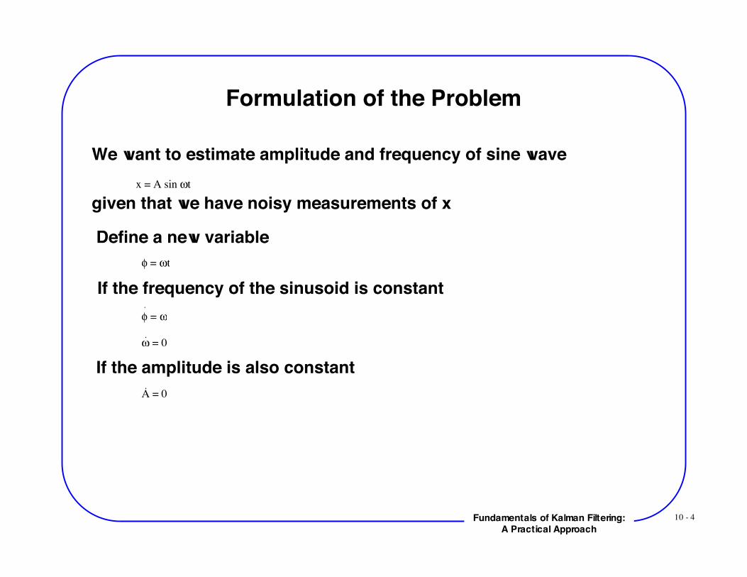
Formulation of the Problem
We want to estimate amplitude and frequency of sine wavex = A sin !t
given that we have noisy measurements of x
Define a new variable! = "t
If the frequency of the sinusoid is constant! = "
! = 0
If the amplitude is also constantA = 0
10 - 5Fundamentals of Kalman Filtering:A Practical Approach
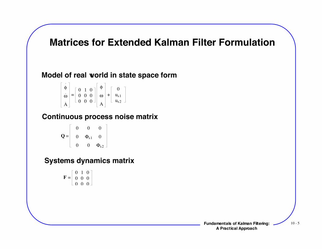
Matrices for Extended Kalman Filter Formulation
Model of real world in state space form!
"
A
=
0 1 0
0 0 0
0 0 0
!
"
A
+
0
us1
us2
Continuous process noise matrix
Systems dynamics matrix
F =
0 1 0
0 0 0
0 0 0
Q =
0 0 0
0 !s1 0
0 0 !s2
10 - 6Fundamentals of Kalman Filtering:A Practical Approach
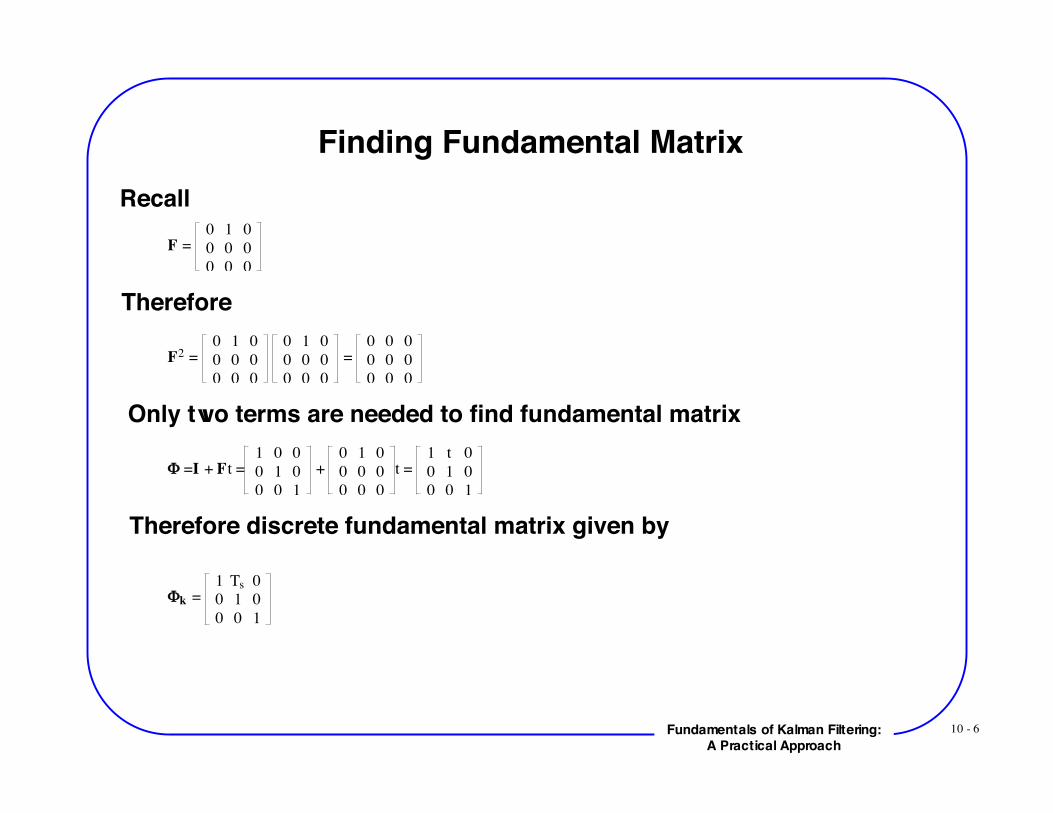
Finding Fundamental MatrixRecall
F =
0 1 0
0 0 0
0 0 0
Therefore
F2 =
0 1 0
0 0 0
0 0 0
0 1 0
0 0 0
0 0 0
=
0 0 0
0 0 0
0 0 0
Only two terms are needed to find fundamental matrix
! =I + Ft =
1 0 0
0 1 0
0 0 1
+
0 1 0
0 0 0
0 0 0
t =
1 t 0
0 1 0
0 0 1
Therefore discrete fundamental matrix given by
!k =
1 Ts 0
0 1 0
0 0 1
10 - 7Fundamentals of Kalman Filtering:A Practical Approach
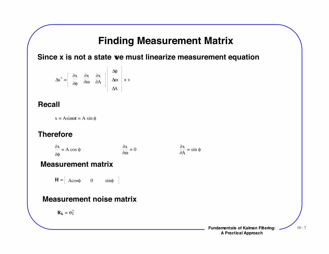
Finding Measurement MatrixSince x is not a state we must linearize measurement equation
!x* = "x
"!
"x
""
"x
"A
!!
!"
!A
+ v
Recallx = Asin!t = A sin "
Therefore!x
!! = A cos !
!x
!! = 0
!x
!A = sin !
Measurement matrix
H = Acos! 0 sin!
Measurement noise matrixRk = !x
2
10 - 8Fundamentals of Kalman Filtering:A Practical Approach
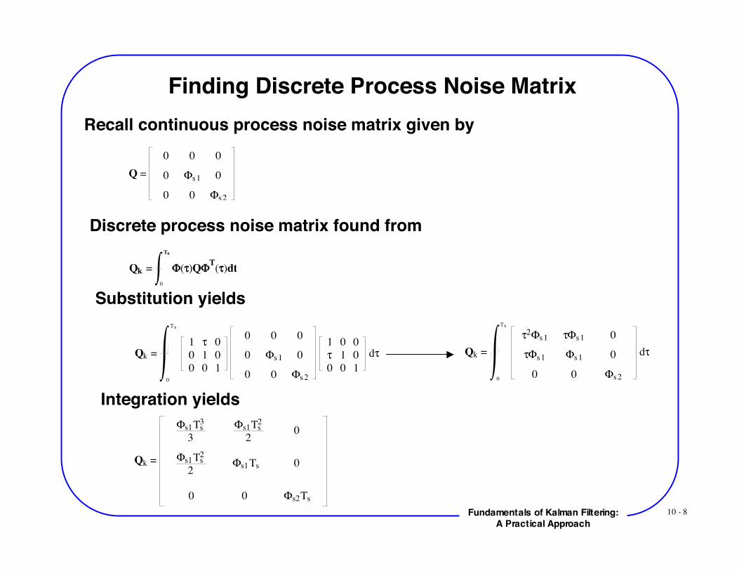
Finding Discrete Process Noise MatrixRecall continuous process noise matrix given by
Q =
0 0 0
0 !s1 0
0 0 !s2
Discrete process noise matrix found from
Qk = !(")Q!T(")dt
0
Ts
Substitution yields
Qk =
1 ! 0
0 1 0
0 0 1
0 0 0
0 "s1 0
0 0 "s2
1 0 0
! 1 0
0 0 1
d!
0
Ts
Qk =
!2"s1 !"s1 0
!"s1 "s1 0
0 0 "s2
d!
0
Ts
Integration yields
Qk =
!s1Ts3
3 !s1Ts
2
2 0
!s1Ts2
2 !s1Ts 0
0 0 !s2Ts
10 - 9Fundamentals of Kalman Filtering:A Practical Approach
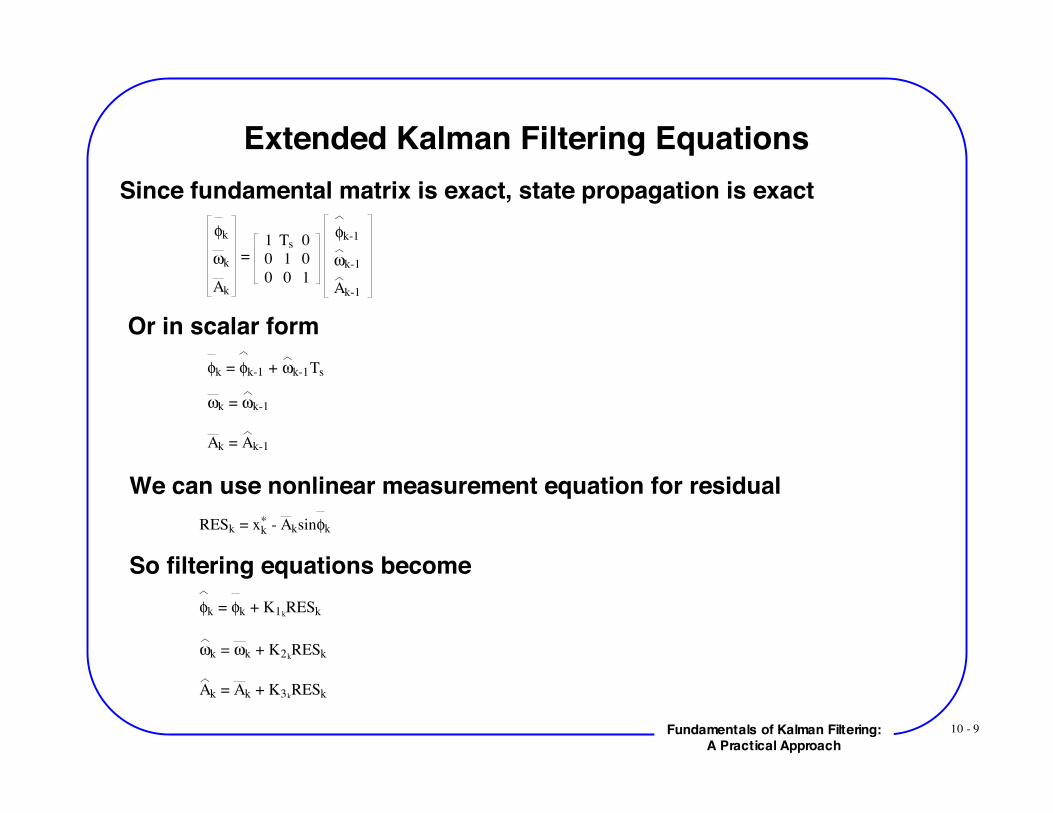
Extended Kalman Filtering EquationsSince fundamental matrix is exact, state propagation is exact
!k
"k
Ak
=
1 Ts 0
0 1 0
0 0 1
!k-1
"k-1
Ak-1
Or in scalar form!k = !k-1 + "k-1Ts
!k = !k-1
Ak = Ak-1
We can use nonlinear measurement equation for residualRESk = xk
* - Aksin!k
So filtering equations become!k = !k + K1k
RESk
!k = !k + K2kRESk
Ak = Ak + K3kRESk
10 - 10Fundamentals of Kalman Filtering:A Practical Approach
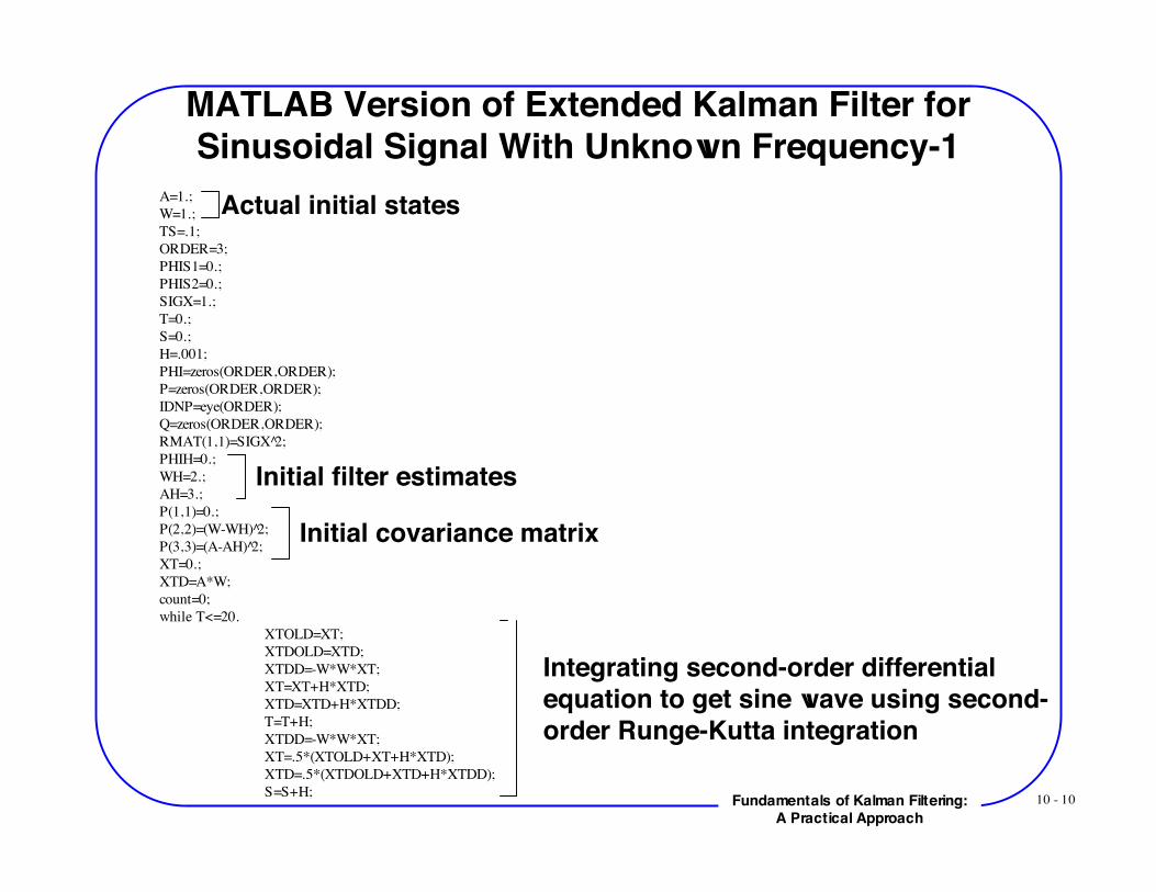
MATLAB Version of Extended Kalman Filter forSinusoidal Signal With Unknown Frequency-1
A=1.;W=1.;TS=.1;ORDER=3;PHIS1=0.;PHIS2=0.;SIGX=1.;T=0.;S=0.;H=.001;PHI=zeros(ORDER,ORDER);P=zeros(ORDER,ORDER);IDNP=eye(ORDER);Q=zeros(ORDER,ORDER);RMAT(1,1)=SIGX 2̂;PHIH=0.;WH=2.;AH=3.;P(1,1)=0.;P(2,2)=(W-WH) 2̂;P(3,3)=(A-AH) 2̂;XT=0.;XTD=A*W;count=0;while T<=20.
XTOLD=XT;XTDOLD=XTD;XTDD=-W*W*XT;
XT=XT+H*XTD; XTD=XTD+H*XTDD;
T=T+H;XTDD=-W*W*XT;
XT=.5*(XTOLD+XT+H*XTD); XTD=.5*(XTDOLD+XTD+H*XTDD);
S=S+H;
Initial filter estimates
Actual initial states
Initial covariance matrix
Integrating second-order differentialequation to get sine wave using second-order Runge-Kutta integration
10 - 11Fundamentals of Kalman Filtering:A Practical Approach
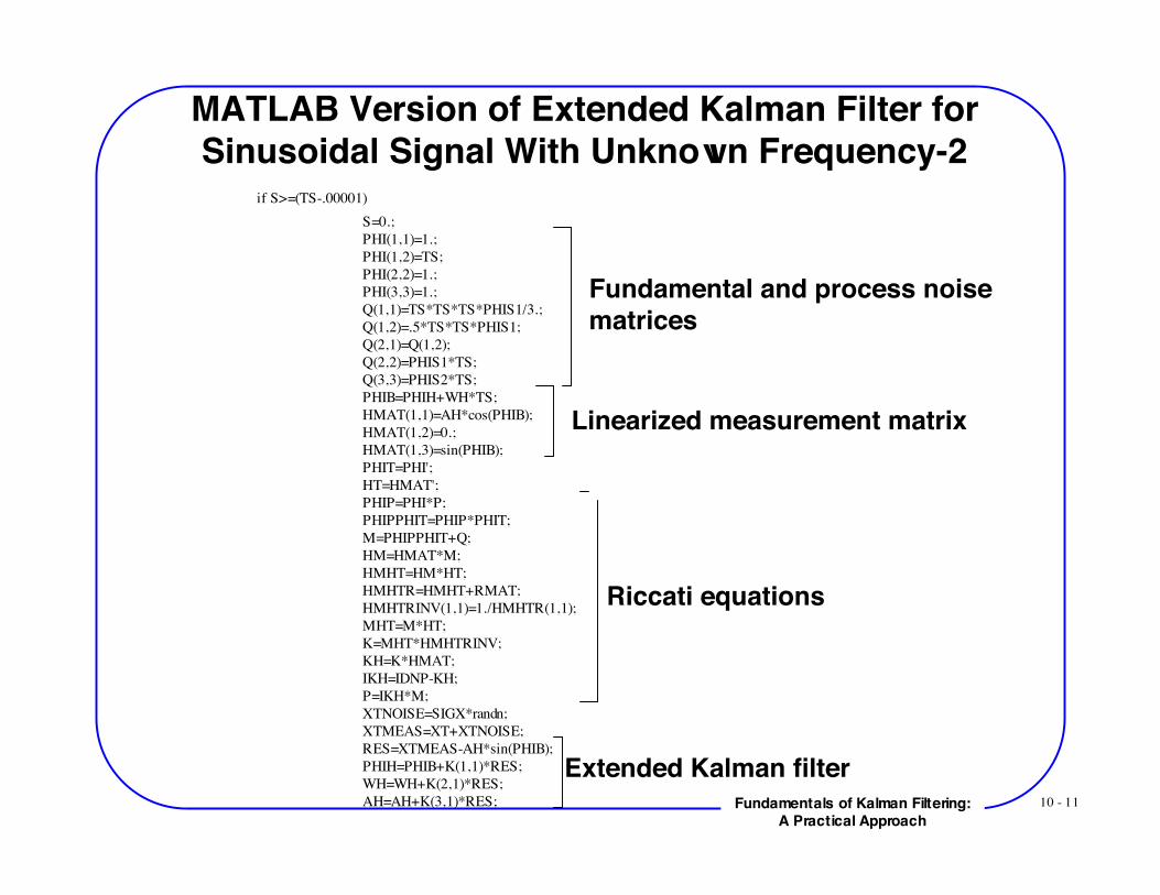
MATLAB Version of Extended Kalman Filter forSinusoidal Signal With Unknown Frequency-2
if S>=(TS-.00001)S=0.;PHI(1,1)=1.;PHI(1,2)=TS;PHI(2,2)=1.;PHI(3,3)=1.;Q(1,1)=TS*TS*TS*PHIS1/3.;Q(1,2)=.5*TS*TS*PHIS1;Q(2,1)=Q(1,2);Q(2,2)=PHIS1*TS;Q(3,3)=PHIS2*TS;PHIB=PHIH+WH*TS;HMAT(1,1)=AH*cos(PHIB);HMAT(1,2)=0.;HMAT(1,3)=sin(PHIB);PHIT=PHI';HT=HMAT';PHIP=PHI*P;PHIPPHIT=PHIP*PHIT;M=PHIPPHIT+Q;HM=HMAT*M;HMHT=HM*HT;HMHTR=HMHT+RMAT;HMHTRINV(1,1)=1./HMHTR(1,1);MHT=M*HT;K=MHT*HMHTRINV;KH=K*HMAT;IKH=IDNP-KH;P=IKH*M;XTNOISE=SIGX*randn;XTMEAS=XT+XTNOISE;RES=XTMEAS-AH*sin(PHIB);PHIH=PHIB+K(1,1)*RES;WH=WH+K(2,1)*RES;AH=AH+K(3,1)*RES;
Fundamental and process noisematrices
Linearized measurement matrix
Riccati equations
Extended Kalman filter
10 - 12Fundamentals of Kalman Filtering:A Practical Approach
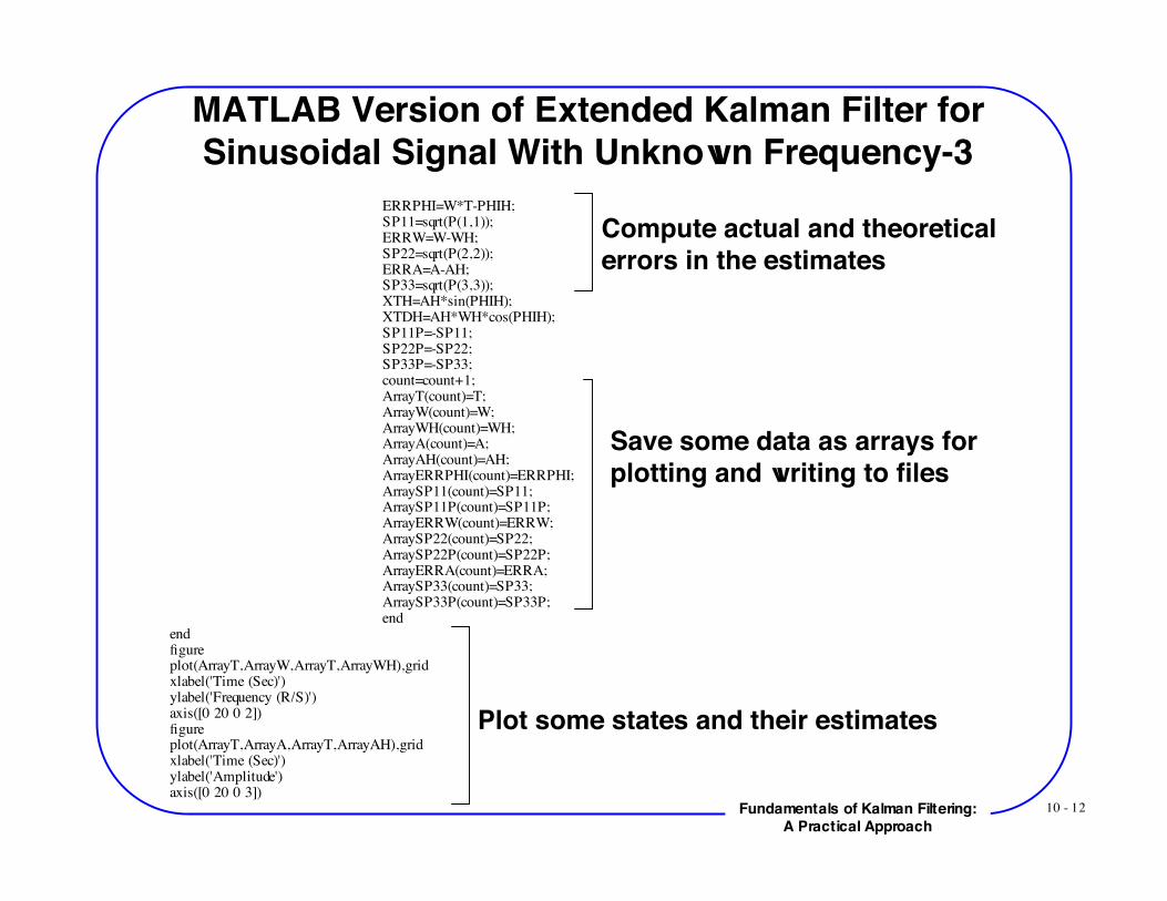
MATLAB Version of Extended Kalman Filter forSinusoidal Signal With Unknown Frequency-3
ERRPHI=W*T-PHIH;SP11=sqrt(P(1,1));ERRW=W-WH;SP22=sqrt(P(2,2));ERRA=A-AH;SP33=sqrt(P(3,3));XTH=AH*sin(PHIH);XTDH=AH*WH*cos(PHIH);SP11P=-SP11;SP22P=-SP22;SP33P=-SP33;count=count+1;ArrayT(count)=T;ArrayW(count)=W;ArrayWH(count)=WH;ArrayA(count)=A;ArrayAH(count)=AH;ArrayERRPHI(count)=ERRPHI;ArraySP11(count)=SP11;ArraySP11P(count)=SP11P;ArrayERRW(count)=ERRW;ArraySP22(count)=SP22;ArraySP22P(count)=SP22P;ArrayERRA(count)=ERRA;ArraySP33(count)=SP33;ArraySP33P(count)=SP33P;end
endfigureplot(ArrayT,ArrayW,ArrayT,ArrayWH),gridxlabel('Time (Sec)')ylabel('Frequency (R/S)')axis([0 20 0 2])figureplot(ArrayT,ArrayA,ArrayT,ArrayAH),gridxlabel('Time (Sec)')ylabel('Amplitude')axis([0 20 0 3])
Compute actual and theoreticalerrors in the estimates
Save some data as arrays forplotting and writing to files
Plot some states and their estimates
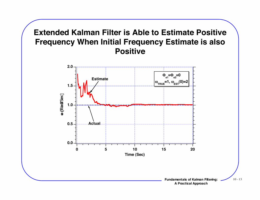
10 - 13Fundamentals of Kalman Filtering:A Practical Approach
Extended Kalman Filter is Able to Estimate PositiveFrequency When Initial Frequency Estimate is also
Positive2.0
1.5
1.0
0.5
0.020151050
Time (Sec)
Φs1
=Φs2
=0ω
TRUE=1, ω
EST(0)=2
Actual
Estimate
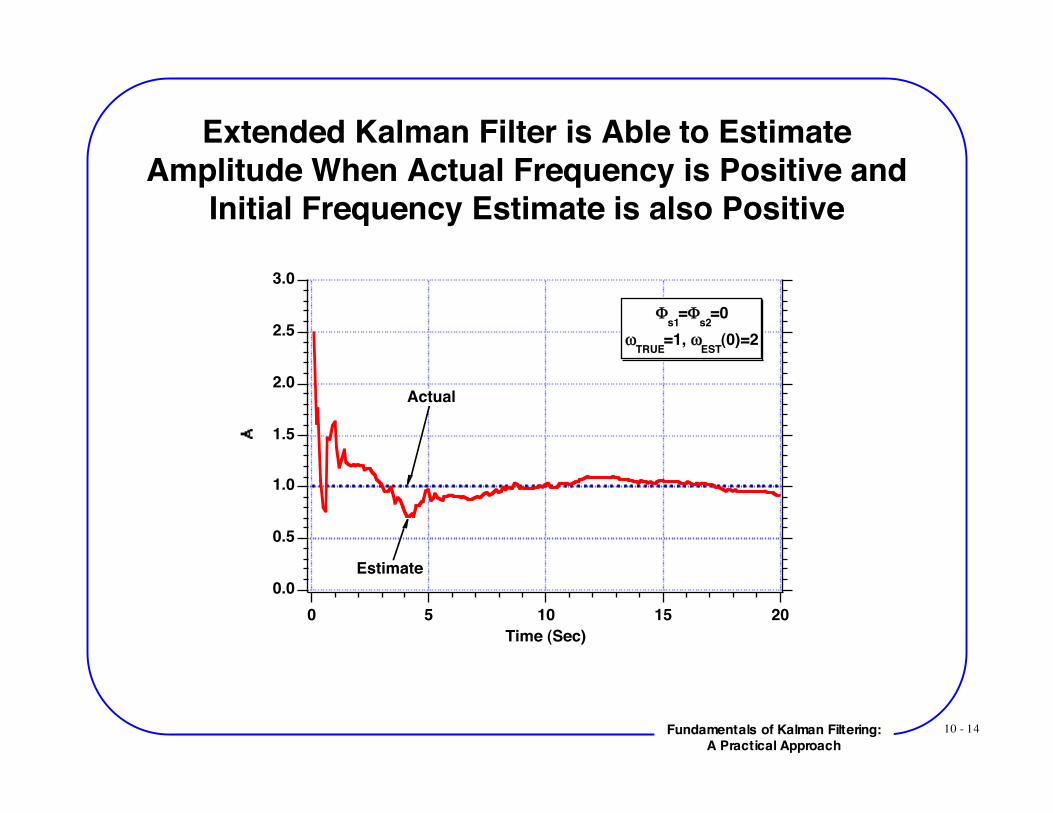
10 - 14Fundamentals of Kalman Filtering:A Practical Approach
Extended Kalman Filter is Able to EstimateAmplitude When Actual Frequency is Positive and
Initial Frequency Estimate is also Positive
3.0
2.5
2.0
1.5
1.0
0.5
0.0
20151050
Time (Sec)
!s1
=!s2
=0
"TRUE
=1, "EST
(0)=2
Actual
Estimate
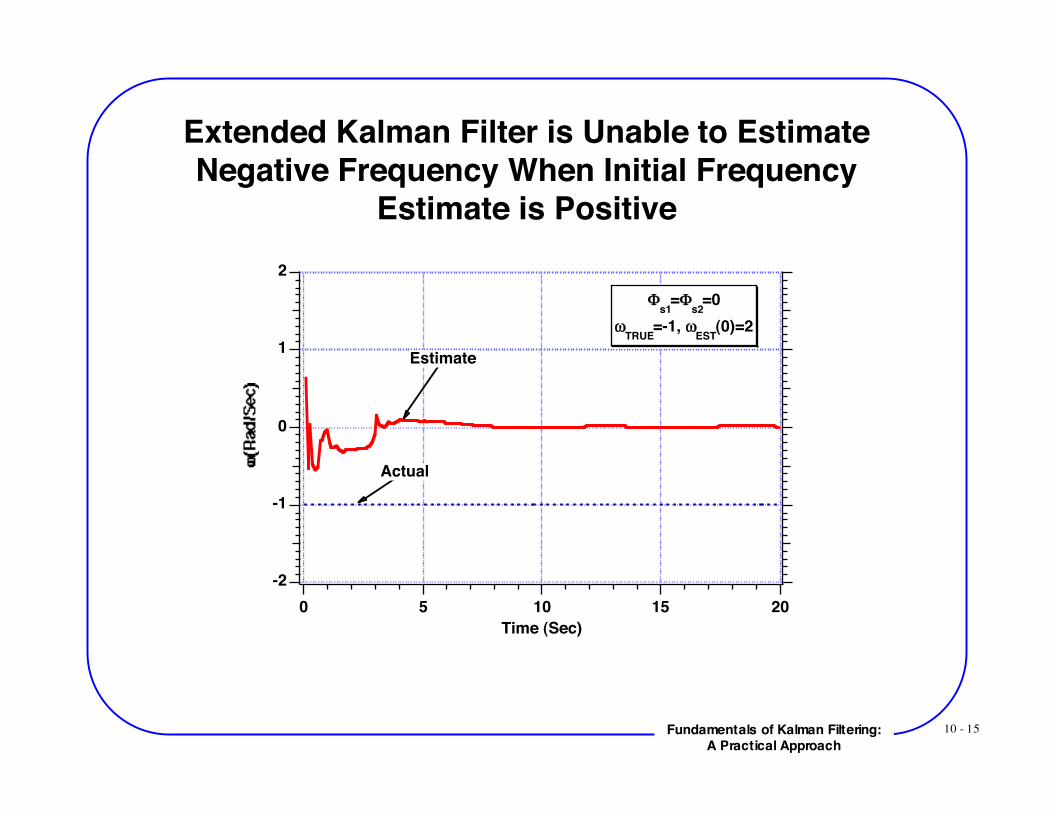
10 - 15Fundamentals of Kalman Filtering:A Practical Approach
Extended Kalman Filter is Unable to EstimateNegative Frequency When Initial Frequency
Estimate is Positive
-2
-1
0
1
2
20151050Time (Sec)
Φs1
=Φs2
=0ω
TRUE=-1, ω
EST(0)=2
Actual
Estimate
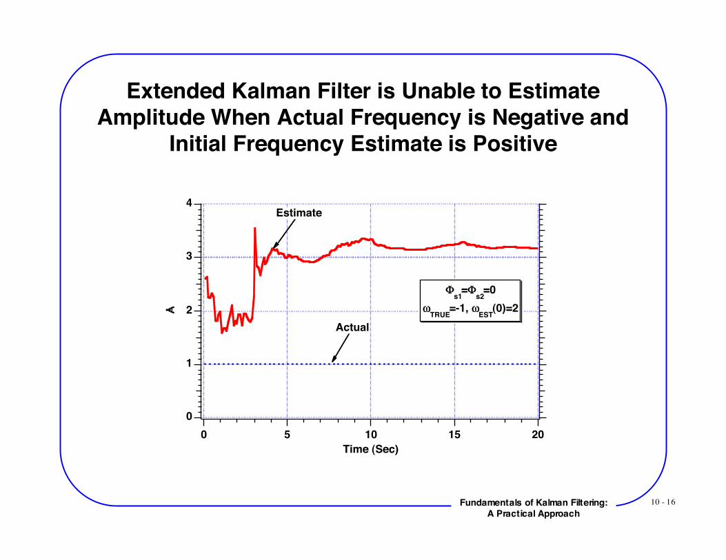
10 - 16Fundamentals of Kalman Filtering:A Practical Approach
Extended Kalman Filter is Unable to EstimateAmplitude When Actual Frequency is Negative and
Initial Frequency Estimate is Positive
4
3
2
1
0
20151050
Time (Sec)
!s1
=!s2
=0
"TRUE
=-1, "EST
(0)=2
Actual
Estimate
10 - 17Fundamentals of Kalman Filtering:A Practical Approach
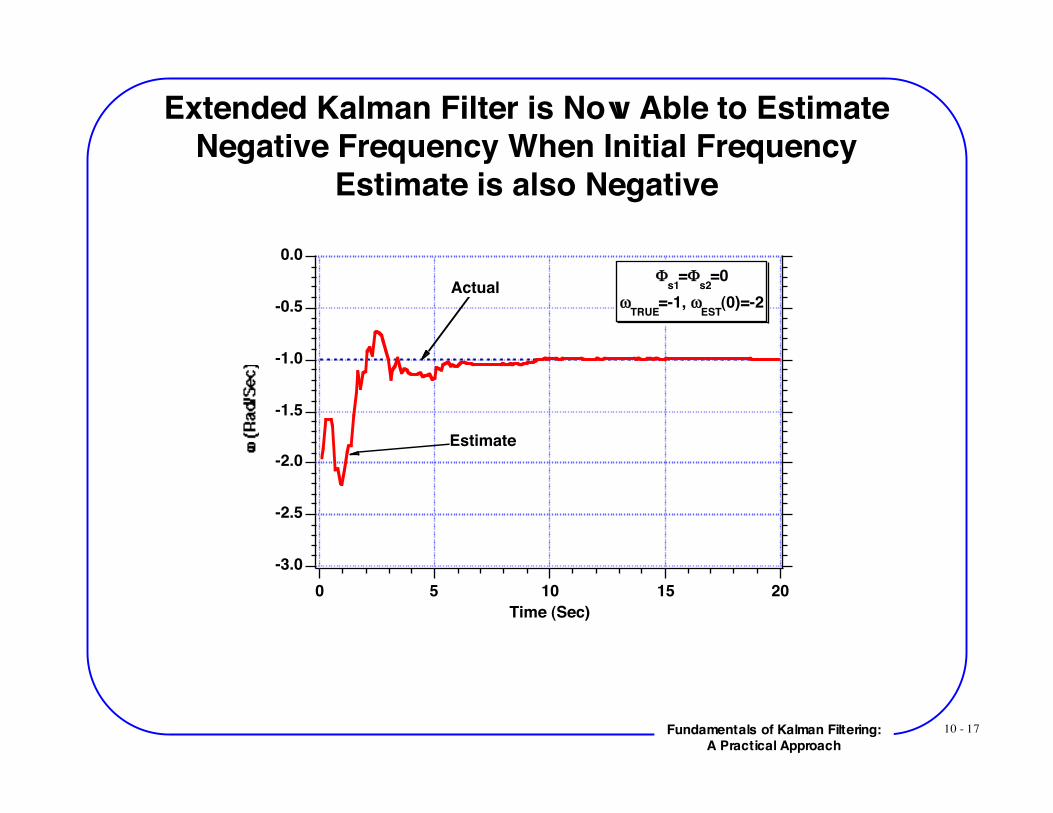
Extended Kalman Filter is Now Able to EstimateNegative Frequency When Initial Frequency
Estimate is also Negative
-3.0
-2.5
-2.0
-1.5
-1.0
-0.5
0.0
20151050Time (Sec)
Φs1
=Φs2
=0ω
TRUE=-1, ω
EST(0)=-2
Actual
Estimate
10 - 18Fundamentals of Kalman Filtering:A Practical Approach
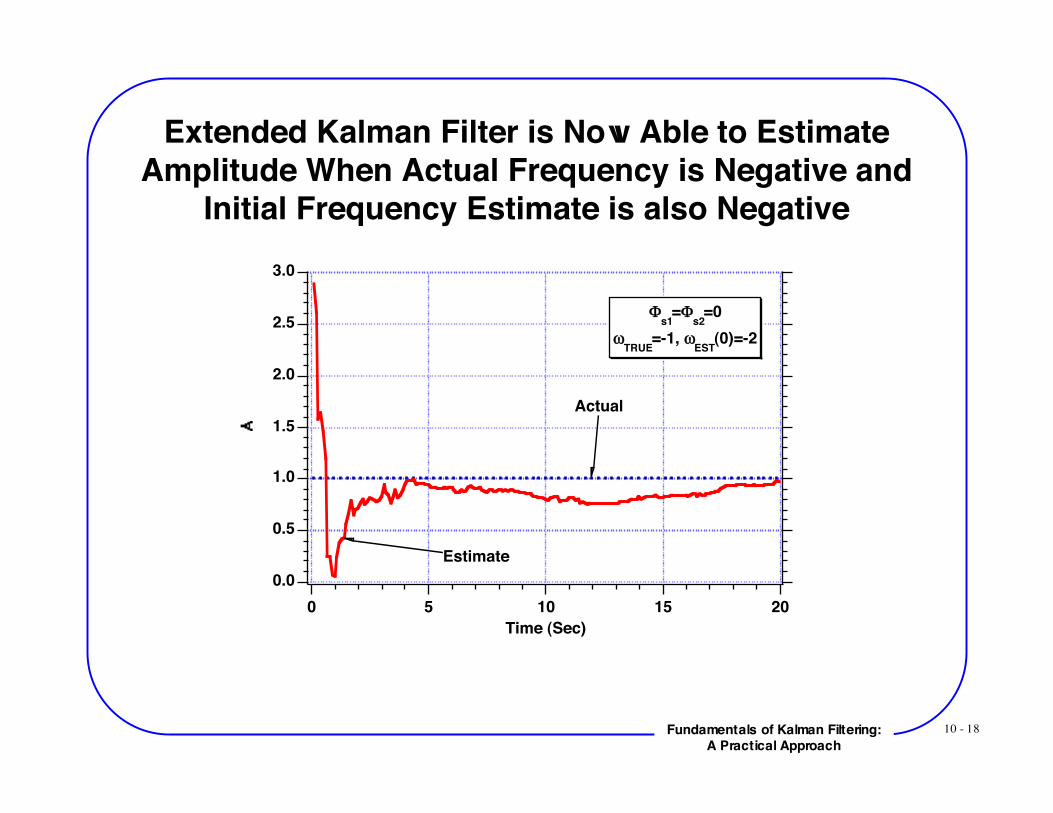
Extended Kalman Filter is Now Able to EstimateAmplitude When Actual Frequency is Negative and
Initial Frequency Estimate is also Negative3.0
2.5
2.0
1.5
1.0
0.5
0.0
20151050
Time (Sec)
!s1
=!s2
=0
"TRUE
=-1, "EST
(0)=-2
Actual
Estimate
10 - 19Fundamentals of Kalman Filtering:A Practical Approach
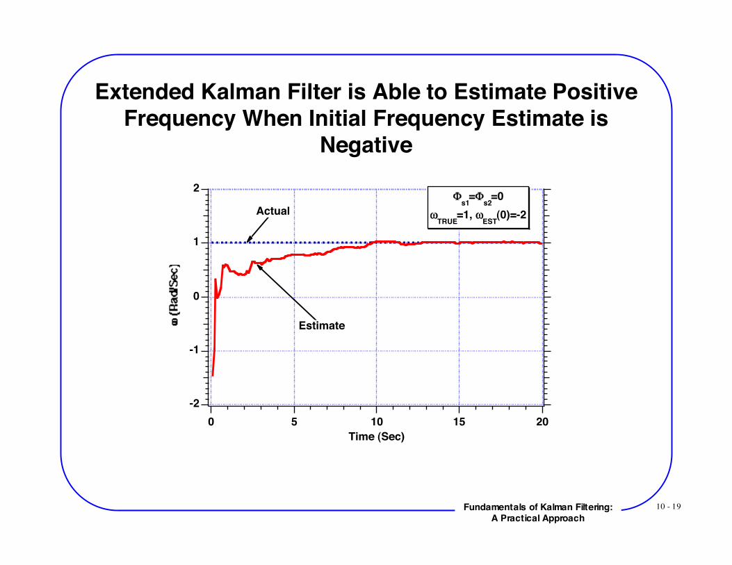
Extended Kalman Filter is Able to Estimate PositiveFrequency When Initial Frequency Estimate is
Negative
-2
-1
0
1
2
20151050Time (Sec)
Φs1
=Φs2
=0ω
TRUE=1, ω
EST(0)=-2Actual
Estimate
10 - 20Fundamentals of Kalman Filtering:A Practical Approach
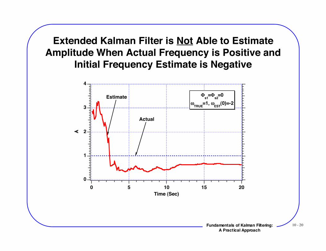
Extended Kalman Filter is Not Able to EstimateAmplitude When Actual Frequency is Positive and
Initial Frequency Estimate is Negative4
3
2
1
0
20151050
Time (Sec)
!s1
=!s2
=0
"TRUE
=1, "EST
(0)=-2
Actual
Estimate
10 - 21Fundamentals of Kalman Filtering:A Practical Approach
Thoughts
• It appears that extended Kalman filter only works when the sign ofthe initial frequency estimate matches the actual frequency• Perhaps we should add process noise because that helped in thepast• Perhaps there is too much measurement noise
10 - 22Fundamentals of Kalman Filtering:A Practical Approach
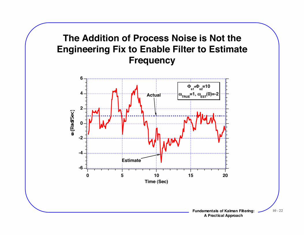
The Addition of Process Noise is Not theEngineering Fix to Enable Filter to Estimate
Frequency
-6
-4
-2
0
2
4
6
20151050Time (Sec)
Φs1
=Φs2
=10ω
TRUE=1, ω
EST(0)=-2Actual
Estimate
10 - 23Fundamentals of Kalman Filtering:A Practical Approach
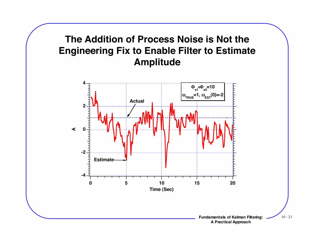
The Addition of Process Noise is Not theEngineering Fix to Enable Filter to Estimate
Amplitude
-4
-2
0
2
4
20151050
Time (Sec)
!s1
=!s2
=10
"TRUE
=1, "EST
(0)=-2
Actual
Estimate
10 - 24Fundamentals of Kalman Filtering:A Practical Approach
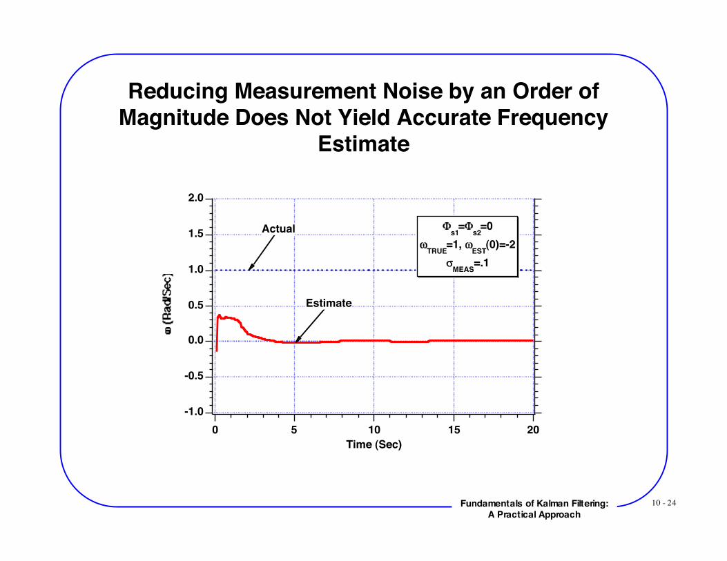
Reducing Measurement Noise by an Order ofMagnitude Does Not Yield Accurate Frequency
Estimate
2.0
1.5
1.0
0.5
0.0
-0.5
-1.020151050
Time (Sec)
Φs1
=Φs2
=0ω
TRUE=1, ω
EST(0)=-2
σMEAS
=.1
Actual
Estimate
10 - 25Fundamentals of Kalman Filtering:A Practical Approach
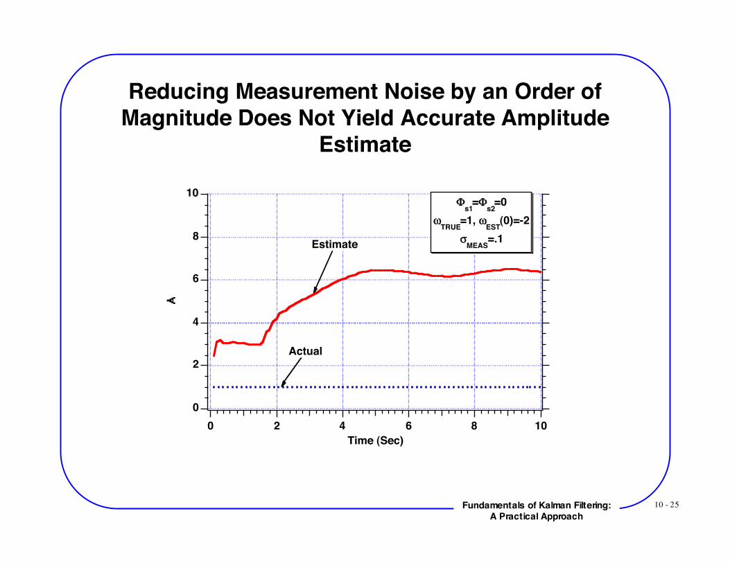
Reducing Measurement Noise by an Order ofMagnitude Does Not Yield Accurate Amplitude
Estimate
10
8
6
4
2
0
1086420
Time (Sec)
!s1
=!s2
=0
"TRUE
=1, "EST
(0)=-2
#MEAS
=.1
Actual
Estimate

10 - 26Fundamentals of Kalman Filtering:A Practical Approach
Two State Extended Kalman Filter With A PrioriInformation
10 - 27Fundamentals of Kalman Filtering:A Practical Approach
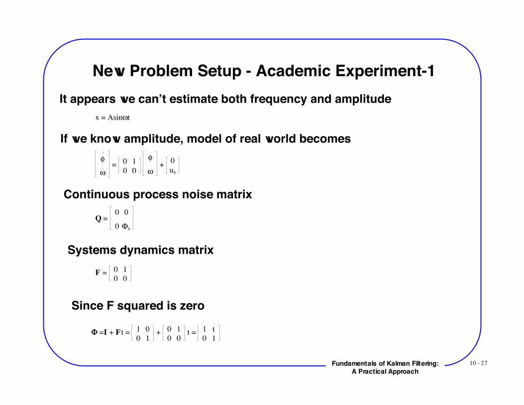
New Problem Setup - Academic Experiment-1It appears we can’t estimate both frequency and amplitude
x = Asin!t
If we know amplitude, model of real world becomes!
" =
0 1
0 0
!
" +
0
us
Continuous process noise matrix
Q = 0 0
0 !s
Systems dynamics matrixF =
0 1
0 0
Since F squared is zero
! =I + F t = 1 0
0 1 +
0 1
0 0 t =
1 t
0 1
10 - 28Fundamentals of Kalman Filtering:A Practical Approach
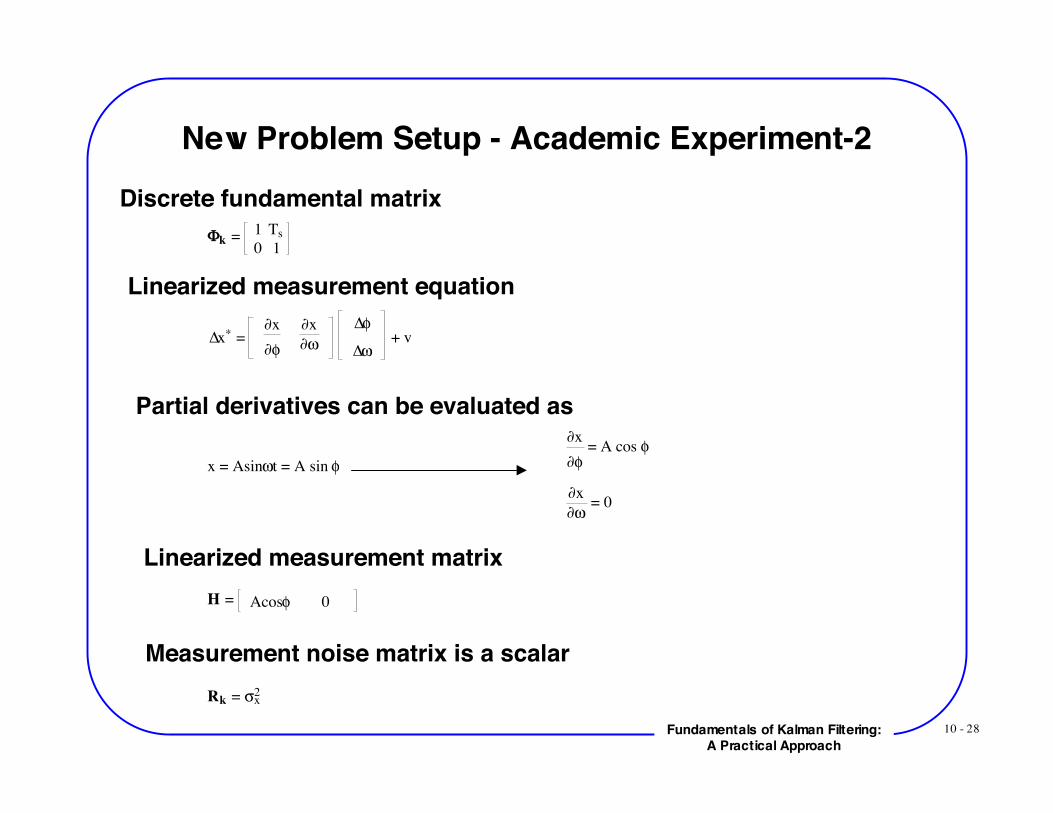
New Problem Setup - Academic Experiment-2Discrete fundamental matrix
!k = 1 Ts
0 1
Linearized measurement equation
!x* = "x
"!
"x
""
!!
!" + v
Partial derivatives can be evaluated as
x = Asin!t = A sin "
!x
!! = A cos !
!x
!! = 0
Linearized measurement matrixH = Acos! 0
Measurement noise matrix is a scalarRk = !x
2
10 - 29Fundamentals of Kalman Filtering:A Practical Approach
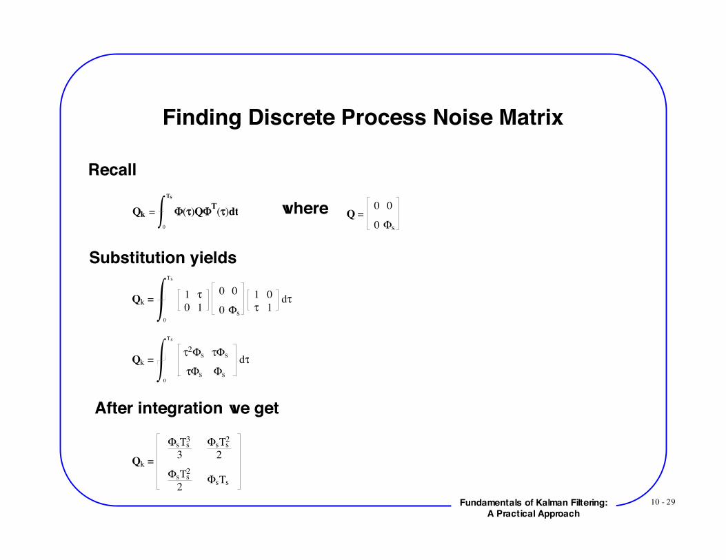
Finding Discrete Process Noise Matrix
Recall
Qk = !(")Q!T(")dt
0
Ts
Q = 0 0
0 !s
where
Substitution yields
Qk = 1 !
0 1
0 0
0 "s
1 0
! 1 d!
0
Ts
Qk = !2"s !"s
!"s "s
d!
0
Ts
After integration we get
Qk =
!sTs3
3 !sTs
2
2
!sTs2
2!sTs
10 - 30Fundamentals of Kalman Filtering:A Practical Approach
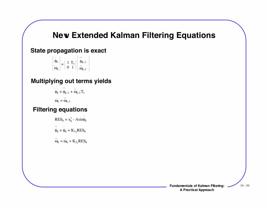
New Extended Kalman Filtering EquationsState propagation is exact
!k
"k
= 1 Ts
0 1 !k-1
"k-1
Multiplying out terms yields!k = !k-1 + "k-1Ts
!k = !k-1
Filtering equationsRESk = xk
* - Asin!k
!k = !k + K1kRESk
!k = !k + K2kRESk
10 - 31Fundamentals of Kalman Filtering:A Practical Approach
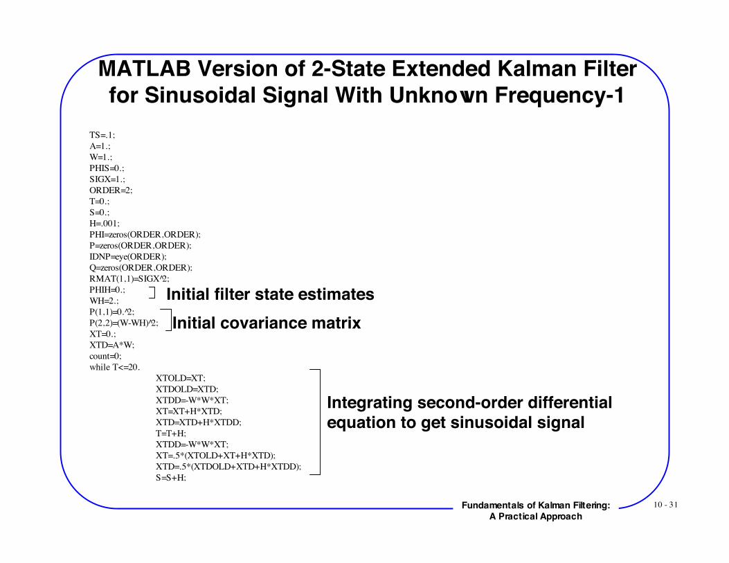
MATLAB Version of 2-State Extended Kalman Filterfor Sinusoidal Signal With Unknown Frequency-1
TS=.1;A=1.;W=1.;PHIS=0.;SIGX=1.;ORDER=2;T=0.;S=0.;H=.001;PHI=zeros(ORDER,ORDER);P=zeros(ORDER,ORDER);IDNP=eye(ORDER);Q=zeros(ORDER,ORDER);RMAT(1,1)=SIGX 2̂;PHIH=0.;WH=2.;P(1,1)=0. 2̂;P(2,2)=(W-WH) 2̂;XT=0.;XTD=A*W;count=0;while T<=20.
XTOLD=XT;XTDOLD=XTD;XTDD=-W*W*XT;
XT=XT+H*XTD; XTD=XTD+H*XTDD;
T=T+H;XTDD=-W*W*XT;
XT=.5*(XTOLD+XT+H*XTD); XTD=.5*(XTDOLD+XTD+H*XTDD);
S=S+H;
Initial filter state estimatesInitial covariance matrix
Integrating second-order differentialequation to get sinusoidal signal
10 - 32Fundamentals of Kalman Filtering:A Practical Approach
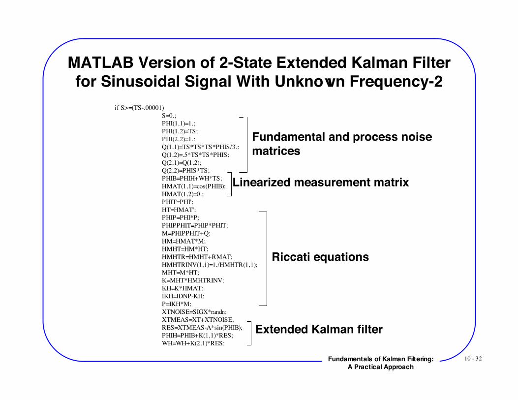
MATLAB Version of 2-State Extended Kalman Filterfor Sinusoidal Signal With Unknown Frequency-2
if S>=(TS-.00001)S=0.;PHI(1,1)=1.;PHI(1,2)=TS;PHI(2,2)=1.;Q(1,1)=TS*TS*TS*PHIS/3.;Q(1,2)=.5*TS*TS*PHIS;Q(2,1)=Q(1,2);Q(2,2)=PHIS*TS;PHIB=PHIH+WH*TS;HMAT(1,1)=cos(PHIB);HMAT(1,2)=0.;PHIT=PHI';HT=HMAT';PHIP=PHI*P;PHIPPHIT=PHIP*PHIT;M=PHIPPHIT+Q;HM=HMAT*M;HMHT=HM*HT;HMHTR=HMHT+RMAT;HMHTRINV(1,1)=1./HMHTR(1,1);MHT=M*HT;K=MHT*HMHTRINV;KH=K*HMAT;IKH=IDNP-KH;P=IKH*M;XTNOISE=SIGX*randn;XTMEAS=XT+XTNOISE;RES=XTMEAS-A*sin(PHIB);PHIH=PHIB+K(1,1)*RES;WH=WH+K(2,1)*RES;
Fundamental and process noisematrices
Linearized measurement matrix
Riccati equations
Extended Kalman filter
10 - 33Fundamentals of Kalman Filtering:A Practical Approach
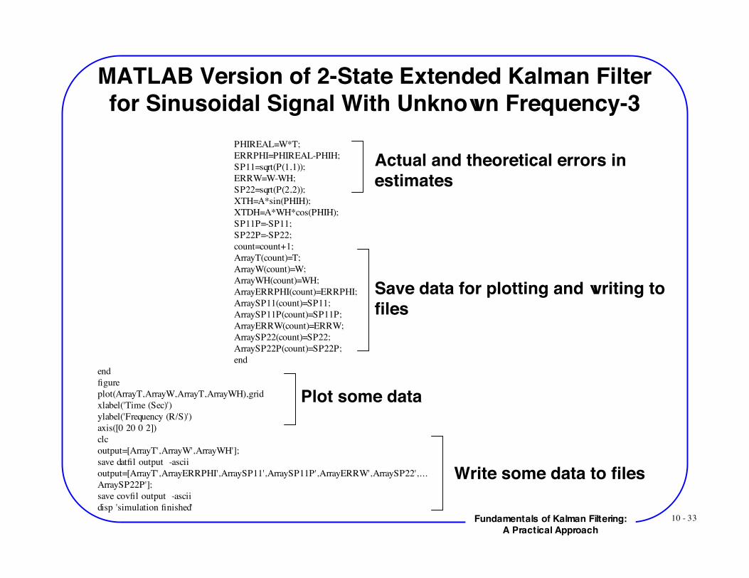
MATLAB Version of 2-State Extended Kalman Filterfor Sinusoidal Signal With Unknown Frequency-3
PHIREAL=W*T;ERRPHI=PHIREAL-PHIH;SP11=sqrt(P(1,1));ERRW=W-WH;SP22=sqrt(P(2,2));XTH=A*sin(PHIH);XTDH=A*WH*cos(PHIH);SP11P=-SP11;SP22P=-SP22;count=count+1;ArrayT(count)=T;ArrayW(count)=W;ArrayWH(count)=WH;ArrayERRPHI(count)=ERRPHI;ArraySP11(count)=SP11;ArraySP11P(count)=SP11P;ArrayERRW(count)=ERRW;ArraySP22(count)=SP22;ArraySP22P(count)=SP22P;end
endfigureplot(ArrayT,ArrayW,ArrayT,ArrayWH),gridxlabel('Time (Sec)')ylabel('Frequency (R/S)')axis([0 20 0 2])clcoutput=[ArrayT',ArrayW',ArrayWH'];save datfil output -asciioutput=[ArrayT',ArrayERRPHI',ArraySP11',ArraySP11P',ArrayERRW',ArraySP22',...ArraySP22P'];save covfil output -asciidisp 'simulation finished'
Actual and theoretical errors inestimates
Save data for plotting and writing tofiles
Plot some data
Write some data to files
10 - 34Fundamentals of Kalman Filtering:A Practical Approach
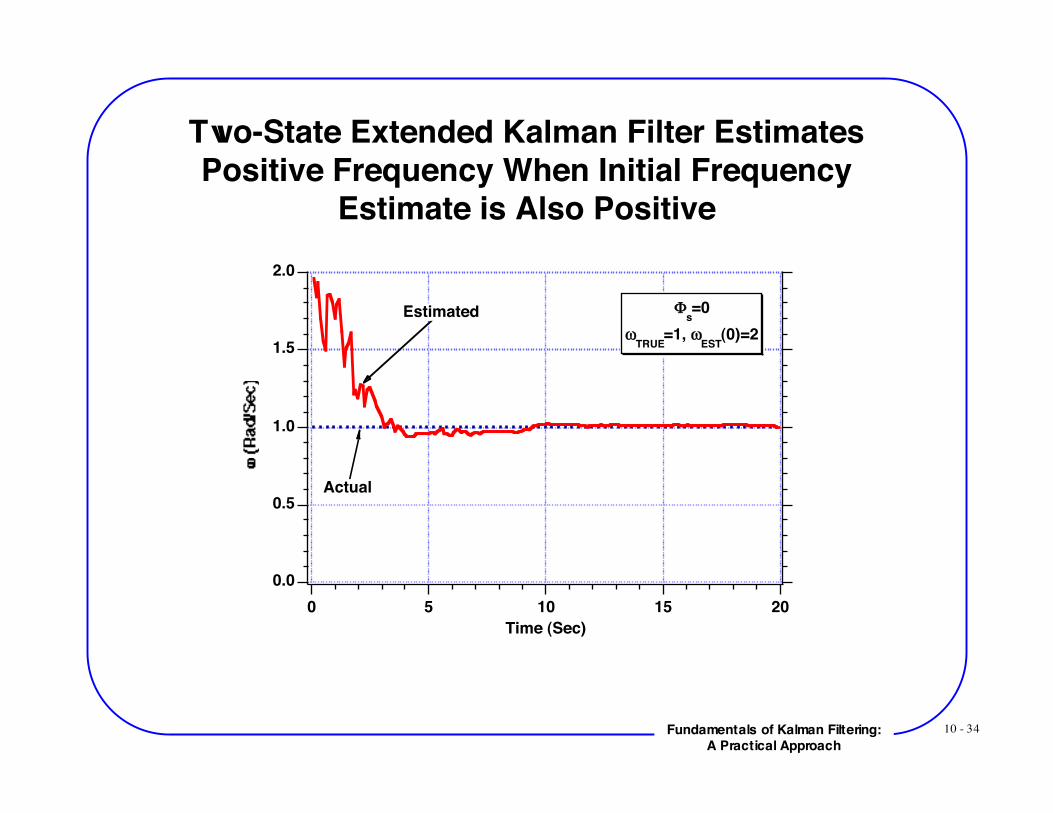
Two-State Extended Kalman Filter EstimatesPositive Frequency When Initial Frequency
Estimate is Also Positive2.0
1.5
1.0
0.5
0.020151050
Time (Sec)
Actual
Estimated Φs=0
ωTRUE
=1, ωEST
(0)=2
10 - 35Fundamentals of Kalman Filtering:A Practical Approach
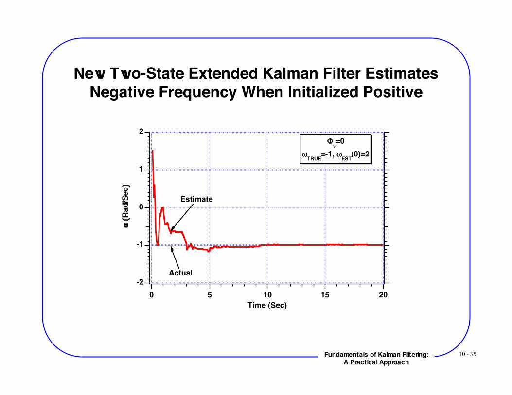
New Two-State Extended Kalman Filter EstimatesNegative Frequency When Initialized Positive
-2
-1
0
1
2
20151050Time (Sec)
Φs=0
ωTRUE
=-1, ωEST
(0)=2
Actual
Estimate
10 - 36Fundamentals of Kalman Filtering:A Practical Approach
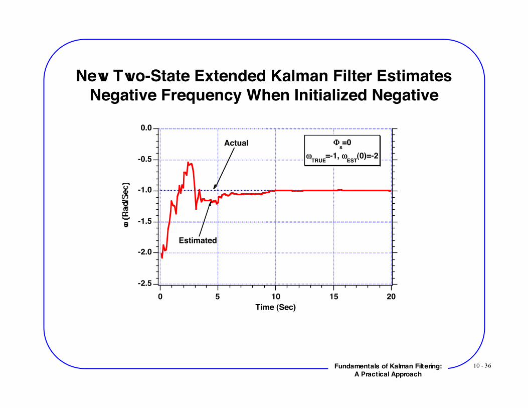
New Two-State Extended Kalman Filter EstimatesNegative Frequency When Initialized Negative
-2.5
-2.0
-1.5
-1.0
-0.5
0.0
20151050Time (Sec)
Φs=0
ωTRUE
=-1, ωEST
(0)=-2Actual
Estimated
10 - 37Fundamentals of Kalman Filtering:A Practical Approach
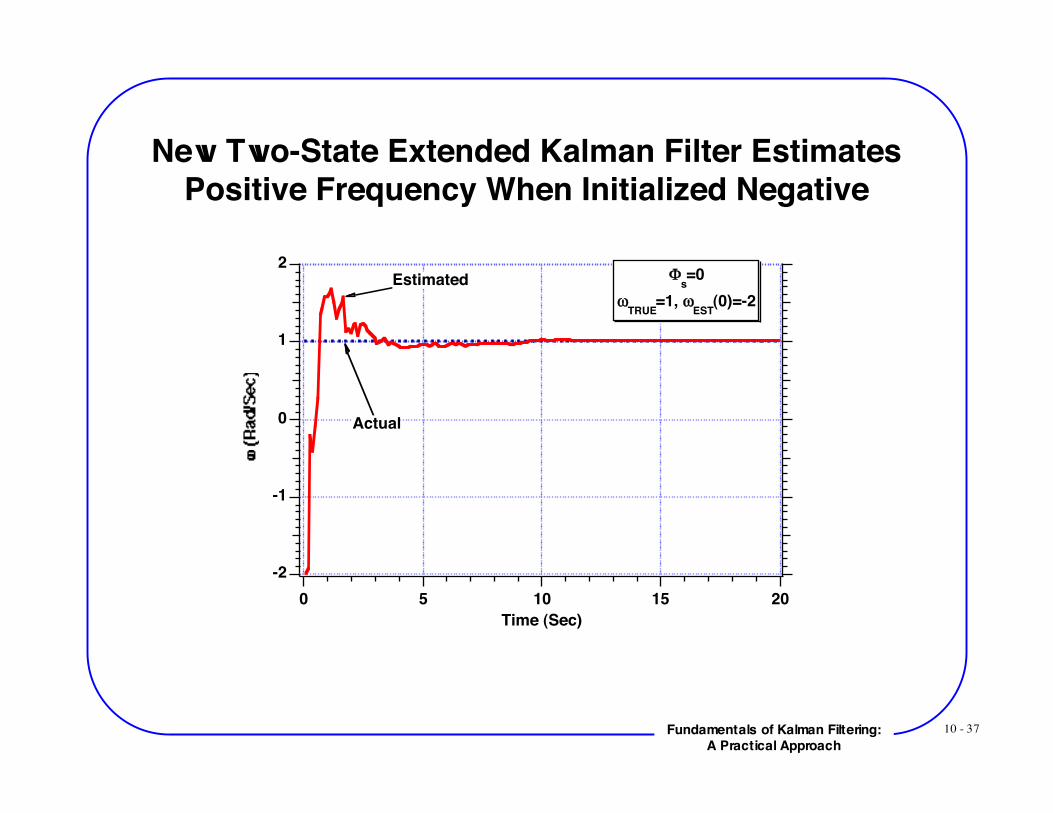
New Two-State Extended Kalman Filter EstimatesPositive Frequency When Initialized Negative
-2
-1
0
1
2
20151050Time (Sec)
Φs=0
ωTRUE
=1, ωEST
(0)=-2
Actual
Estimated
10 - 38Fundamentals of Kalman Filtering:A Practical Approach
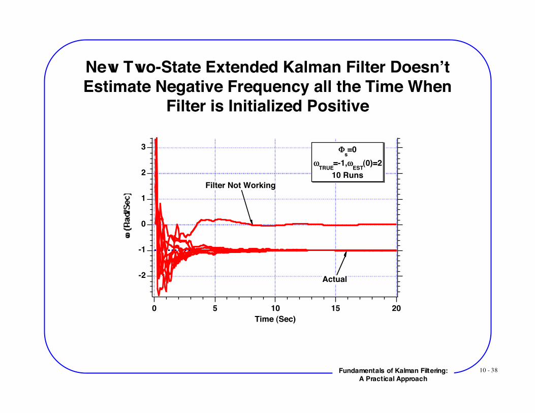
New Two-State Extended Kalman Filter Doesn’tEstimate Negative Frequency all the Time When
Filter is Initialized Positive
3
2
1
0
-1
-2
20151050Time (Sec)
Φs=0
ωTRUE
=-1,ωEST
(0)=210 Runs
Actual
Filter Not Working
10 - 39Fundamentals of Kalman Filtering:A Practical Approach
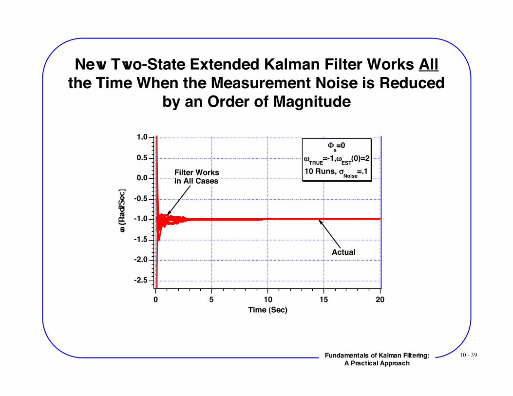
New Two-State Extended Kalman Filter Works Allthe Time When the Measurement Noise is Reduced
by an Order of Magnitude
-2.5
-2.0
-1.5
-1.0
-0.5
0.0
0.5
1.0
20151050Time (Sec)
Φs=0
ωTRUE
=-1,ωEST
(0)=210 Runs, σ
Noise=.1Filter Works
in All Cases
Actual
10 - 40Fundamentals of Kalman Filtering:A Practical Approach
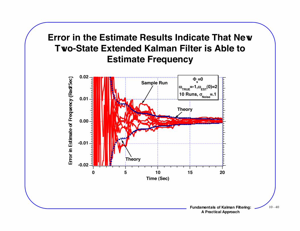
Error in the Estimate Results Indicate That NewTwo-State Extended Kalman Filter is Able to
Estimate Frequency
-0.02
-0.01
0.00
0.01
0.02
20151050
Time (Sec)
!s=0
"TRUE
=-1,"EST
(0)=2
10 Runs, #Noise
=.1
Sample Run
Theory
Theory
10 - 41Fundamentals of Kalman Filtering:A Practical Approach
Alternate Extended Kalman Filter For SinusoidalSignal
10 - 42Fundamentals of Kalman Filtering:A Practical Approach
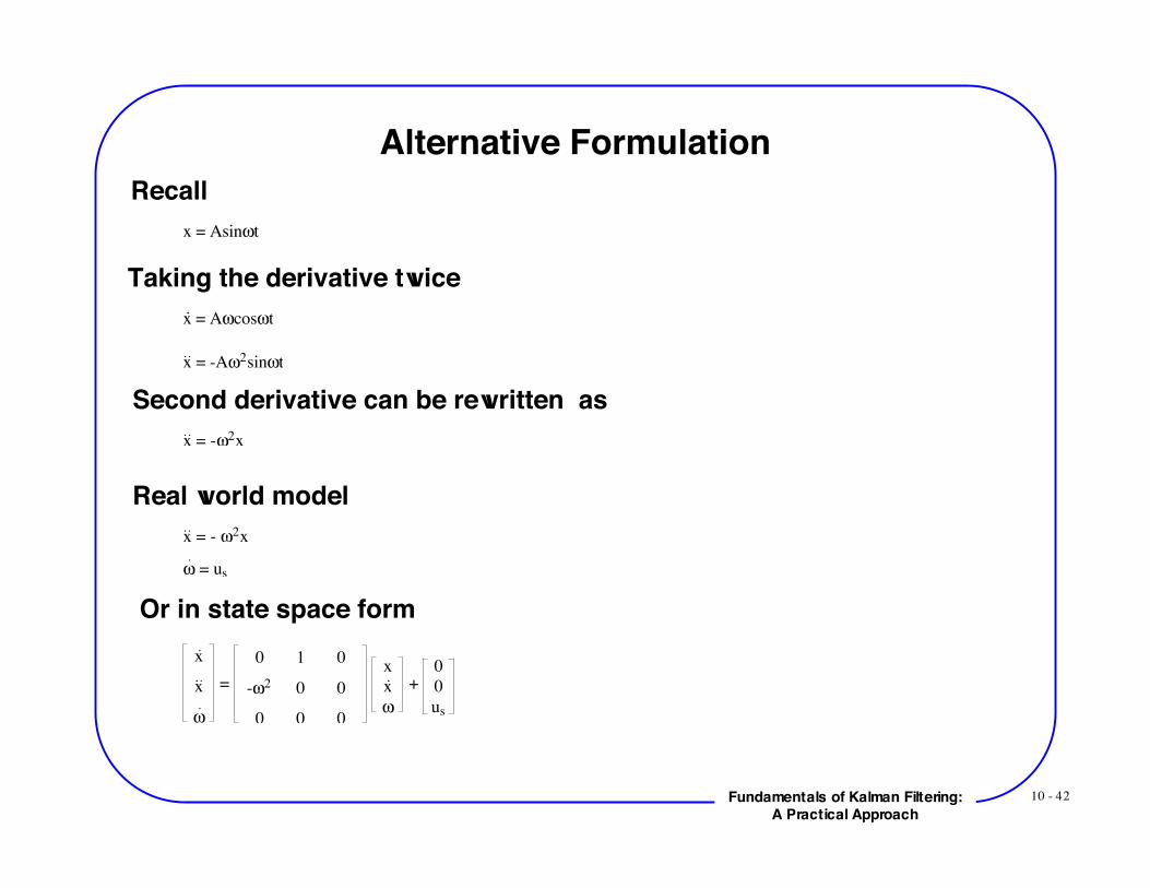
Alternative FormulationRecall
x = Asin!t
Taking the derivative twicex = A!cos!t
x = -A!2sin!t
Second derivative can be rewritten asx = -!2
x
Real world modelx = - !2
x
! = us
Or in state space formx
x
!
=
0 1 0
-!2 0 0
0 0 0
x
x
!
+
0
0
us
10 - 43Fundamentals of Kalman Filtering:A Practical Approach
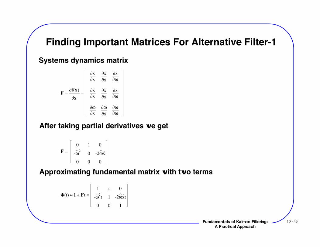
Finding Important Matrices For Alternative Filter-1Systems dynamics matrix
F = !f(x)
!x
=
!x
!x
!x
!x
!x
!"
!x
!x
!x
!x
!x
!"
!"
!x
!"
!x
!"
!"
After taking partial derivatives we get
F =
0 1 0
-!2
0 -2!x
0 0 0
Approximating fundamental matrix with two terms
!(t) " I + Ft =
1 t 0
-#2t 1 -2#xt
0 0 1
10 - 44Fundamentals of Kalman Filtering:A Practical Approach
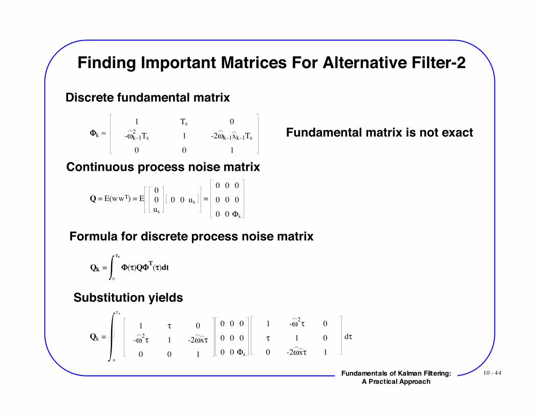
Finding Important Matrices For Alternative Filter-2
Discrete fundamental matrix
!k "
1 Ts 0
-#k-1
2Ts 1 -2#k-1xk-1Ts
0 0 1
Continuous process noise matrix
Q = E(wwT) = E 0
0
us
0 0 us =
0 0 0
0 0 0
0 0 !s
Formula for discrete process noise matrix
Qk = !(")Q!T(")dt
0
Ts
Substitution yields
Qk =
1 ! 0
-"2! 1 -2"x!
0 0 1
0 0 0
0 0 0
0 0 #s
1 -"2! 0
! 1 0
0 -2"x! 1
d!
0
Ts
Fundamental matrix is not exact
10 - 45Fundamentals of Kalman Filtering:A Practical Approach
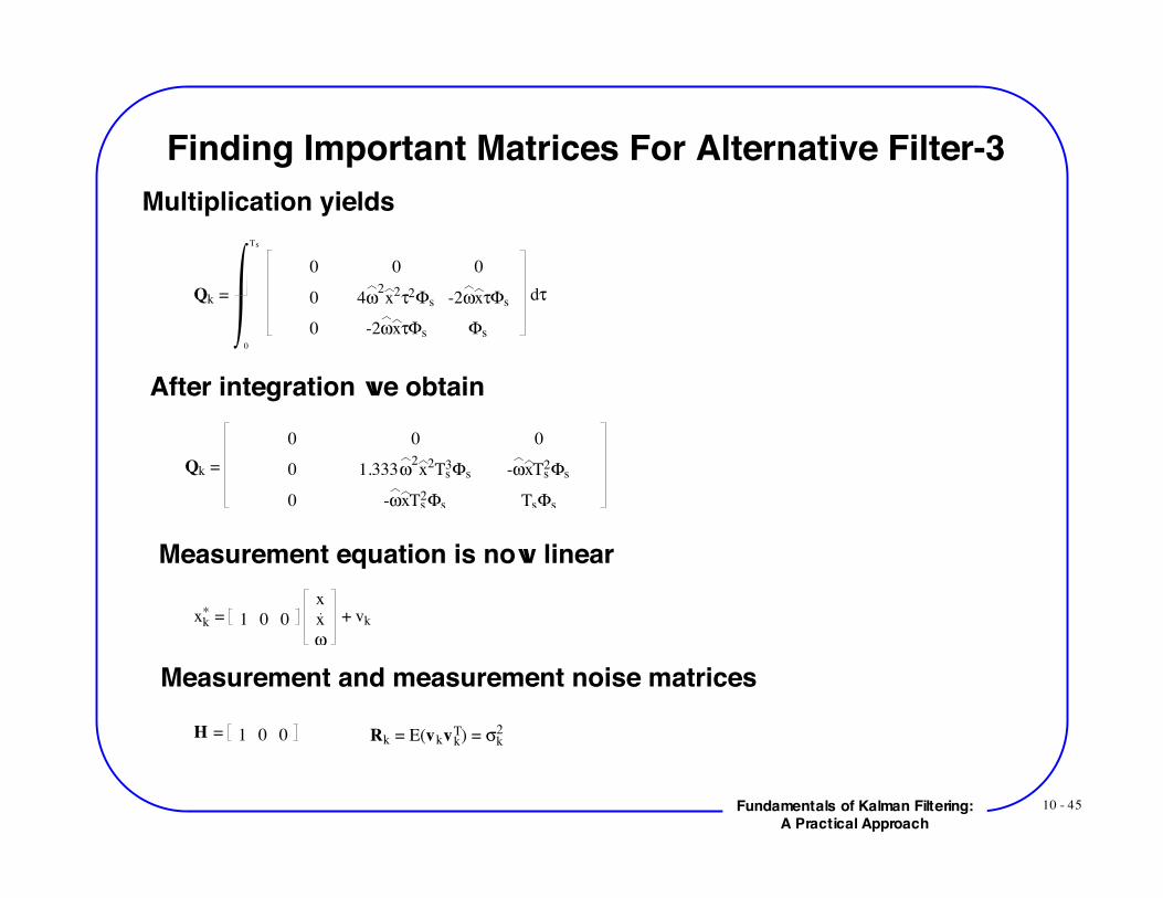
Finding Important Matrices For Alternative Filter-3Multiplication yields
Qk =
0 0 0
0 4!2x
2"2#s -2!x"#s
0 -2!x"#s #s
d"
0
Ts
After integration we obtain
Qk =
0 0 0
0 1.333!2x
2Ts
3"s -!xTs2"s
0 -!xTs2"s Ts"s
Measurement equation is now linear
xk* = 1 0 0
x
x
!
+ vk
Measurement and measurement noise matrices
H = 1 0 0 Rk = E(vkvkT) = !k
2
10 - 46Fundamentals of Kalman Filtering:A Practical Approach
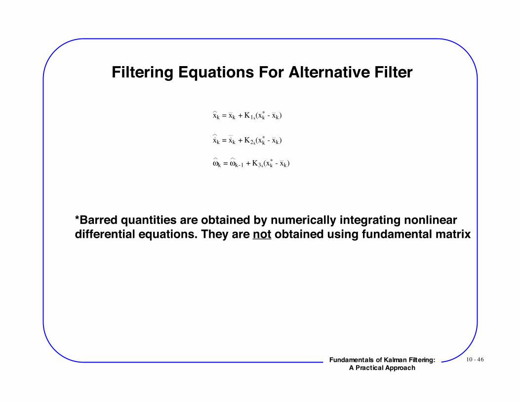
Filtering Equations For Alternative Filter
xk = xk + K1k(xk
* - xk)
xk = xk + K2k(xk
* - xk)
!k = !k-1 + K3k(xk
* - xk)
*Barred quantities are obtained by numerically integrating nonlineardifferential equations. They are not obtained using fundamental matrix
10 - 47Fundamentals of Kalman Filtering:A Practical Approach
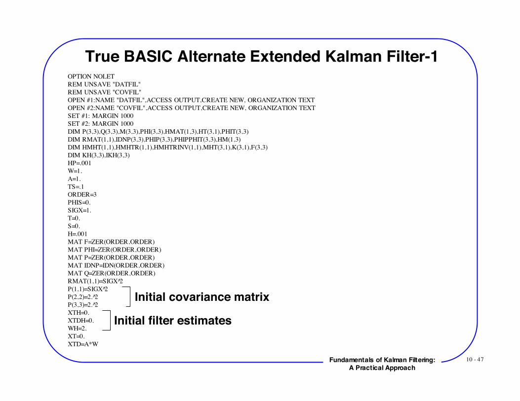
True BASIC Alternate Extended Kalman Filter-1OPTION NOLETREM UNSAVE "DATFIL"REM UNSAVE "COVFIL"OPEN #1:NAME "DATFIL",ACCESS OUTPUT,CREATE NEW, ORGANIZATION TEXTOPEN #2:NAME "COVFIL",ACCESS OUTPUT,CREATE NEW, ORGANIZATION TEXTSET #1: MARGIN 1000SET #2: MARGIN 1000DIM P(3,3),Q(3,3),M(3,3),PHI(3,3),HMAT(1,3),HT(3,1),PHIT(3,3)DIM RMAT(1,1),IDNP(3,3),PHIP(3,3),PHIPPHIT(3,3),HM(1,3)DIM HMHT(1,1),HMHTR(1,1),HMHTRINV(1,1),MHT(3,1),K(3,1),F(3,3)DIM KH(3,3),IKH(3,3)HP=.001W=1.A=1.TS=.1ORDER=3PHIS=0.SIGX=1.T=0.S=0.H=.001MAT F=ZER(ORDER,ORDER)MAT PHI=ZER(ORDER,ORDER)MAT P=ZER(ORDER,ORDER)MAT IDNP=IDN(ORDER,ORDER)MAT Q=ZER(ORDER,ORDER)RMAT(1,1)=SIGX 2̂P(1,1)=SIGX 2̂P(2,2)=2. 2̂P(3,3)=2. 2̂XTH=0.XTDH=0.WH=2.XT=0.XTD=A*W
Initial covariance matrix
Initial filter estimates
10 - 48Fundamentals of Kalman Filtering:A Practical Approach
True BASIC Alternate Extended Kalman Filter-2DO WHILE T<=20.
XTOLD=XTXTDOLD=XTDXTDD=-W*W*XT
XT=XT+H*XTD XTD=XTD+H*XTDD
T=T+HXTDD=-W*W*XT
XT=.5*(XTOLD+XT+H*XTD) XTD=.5*(XTDOLD+XTD+H*XTDD)
S=S+HIF S>=(TS-.00001) THEN
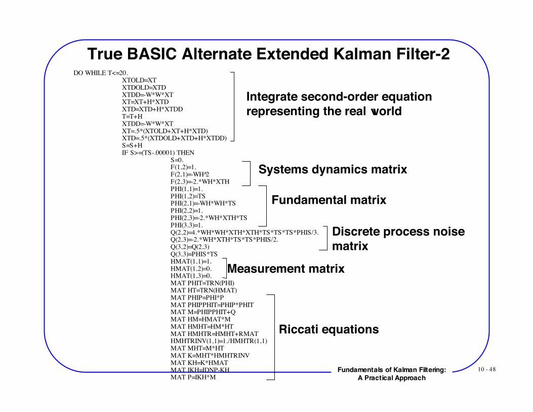
S=0.F(1,2)=1.F(2,1)=-WH 2̂F(2,3)=-2.*WH*XTHPHI(1,1)=1.PHI(1,2)=TSPHI(2,1)=-WH*WH*TSPHI(2,2)=1.PHI(2,3)=-2.*WH*XTH*TSPHI(3,3)=1.Q(2,2)=4.*WH*WH*XTH*XTH*TS*TS*TS*PHIS/3.Q(2,3)=-2.*WH*XTH*TS*TS*PHIS/2.Q(3,2)=Q(2,3)Q(3,3)=PHIS*TSHMAT(1,1)=1.HMAT(1,2)=0.HMAT(1,3)=0.MAT PHIT=TRN(PHI)MAT HT=TRN(HMAT)MAT PHIP=PHI*PMAT PHIPPHIT=PHIP*PHITMAT M=PHIPPHIT+QMAT HM=HMAT*MMAT HMHT=HM*HTMAT HMHTR=HMHT+RMATHMHTRINV(1,1)=1./HMHTR(1,1)MAT MHT=M*HTMAT K=MHT*HMHTRINVMAT KH=K*HMATMAT IKH=IDNP-KHMAT P=IKH*M
Integrate second-order equationrepresenting the real world
Systems dynamics matrix
Fundamental matrix
Discrete process noisematrix
Measurement matrix
Riccati equations
10 - 49Fundamentals of Kalman Filtering:A Practical Approach
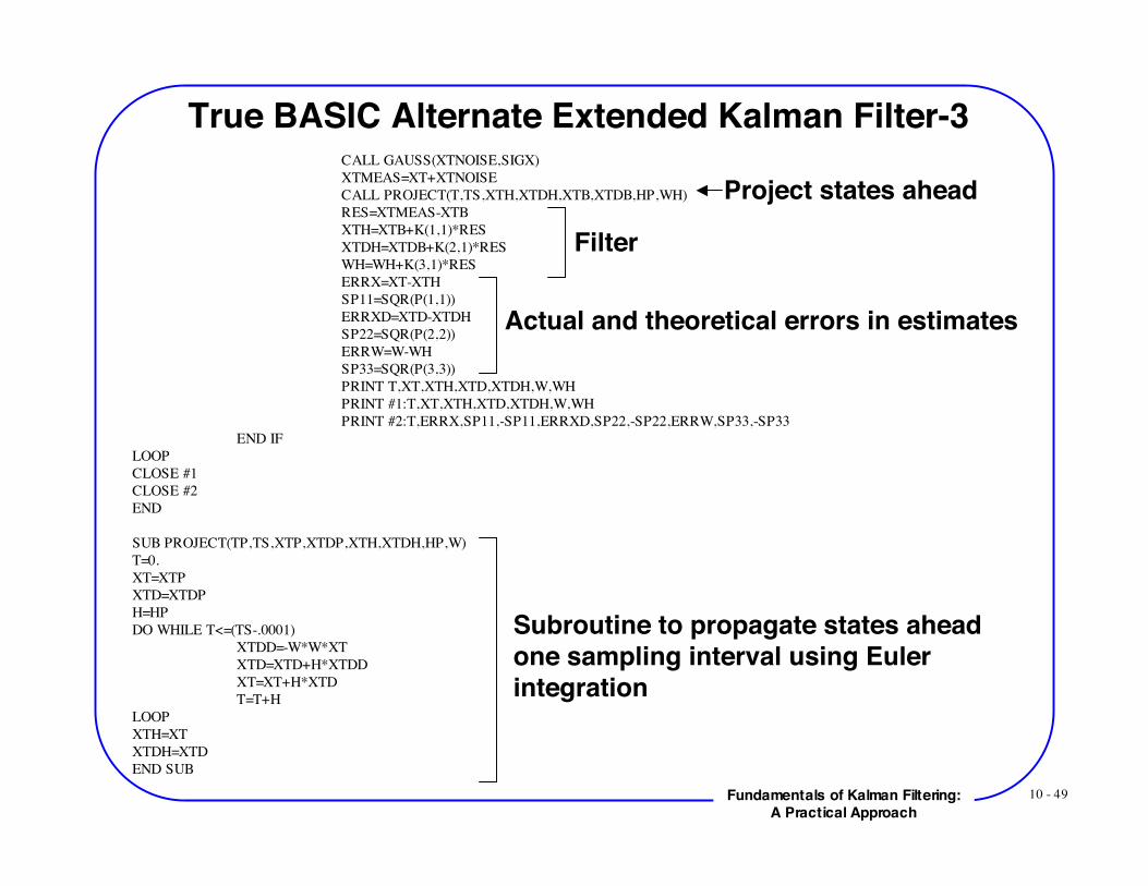
True BASIC Alternate Extended Kalman Filter-3CALL GAUSS(XTNOISE,SIGX)XTMEAS=XT+XTNOISECALL PROJECT(T,TS,XTH,XTDH,XTB,XTDB,HP,WH)RES=XTMEAS-XTBXTH=XTB+K(1,1)*RESXTDH=XTDB+K(2,1)*RESWH=WH+K(3,1)*RESERRX=XT-XTHSP11=SQR(P(1,1))ERRXD=XTD-XTDHSP22=SQR(P(2,2))ERRW=W-WHSP33=SQR(P(3,3))PRINT T,XT,XTH,XTD,XTDH,W,WHPRINT #1:T,XT,XTH,XTD,XTDH,W,WHPRINT #2:T,ERRX,SP11,-SP11,ERRXD,SP22,-SP22,ERRW,SP33,-SP33
END IFLOOPCLOSE #1CLOSE #2END
SUB PROJECT(TP,TS,XTP,XTDP,XTH,XTDH,HP,W)T=0.XT=XTPXTD=XTDPH=HPDO WHILE T<=(TS-.0001)
XTDD=-W*W*XTXTD=XTD+H*XTDDXT=XT+H*XTDT=T+H
LOOPXTH=XTXTDH=XTDEND SUB
Subroutine to propagate states aheadone sampling interval using Eulerintegration
Project states ahead
Filter
Actual and theoretical errors in estimates
10 - 50Fundamentals of Kalman Filtering:A Practical Approach
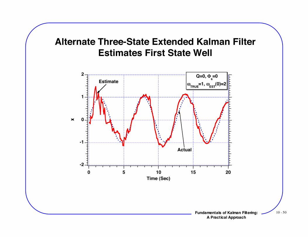
Alternate Three-State Extended Kalman FilterEstimates First State Well
-2
-1
0
1
2
20151050
Time (Sec)
Actual
EstimateQ=0, !
s=0
"TRUE
=1, "EST
(0)=2
10 - 51Fundamentals of Kalman Filtering:A Practical Approach
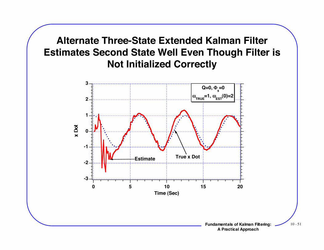
Alternate Three-State Extended Kalman FilterEstimates Second State Well Even Though Filter is
Not Initialized Correctly
-3
-2
-1
0
1
2
3
20151050
Time (Sec)
True x DotEstimate
Q=0, !s=0
"TRUE
=1, "EST
(0)=2
10 - 52Fundamentals of Kalman Filtering:A Practical Approach
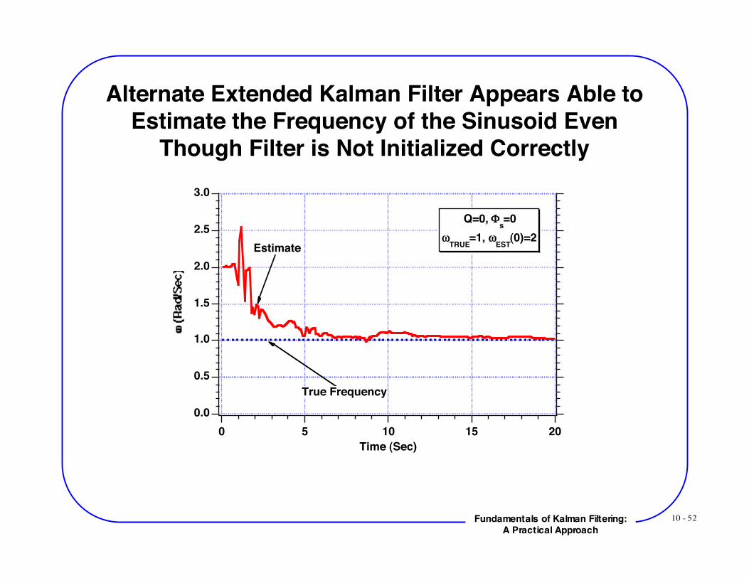
Alternate Extended Kalman Filter Appears Able toEstimate the Frequency of the Sinusoid Even
Though Filter is Not Initialized Correctly3.0
2.5
2.0
1.5
1.0
0.5
0.020151050
Time (Sec)
True Frequency
Estimate
Q=0, Φs=0
ωTRUE
=1, ωEST
(0)=2
10 - 53Fundamentals of Kalman Filtering:A Practical Approach
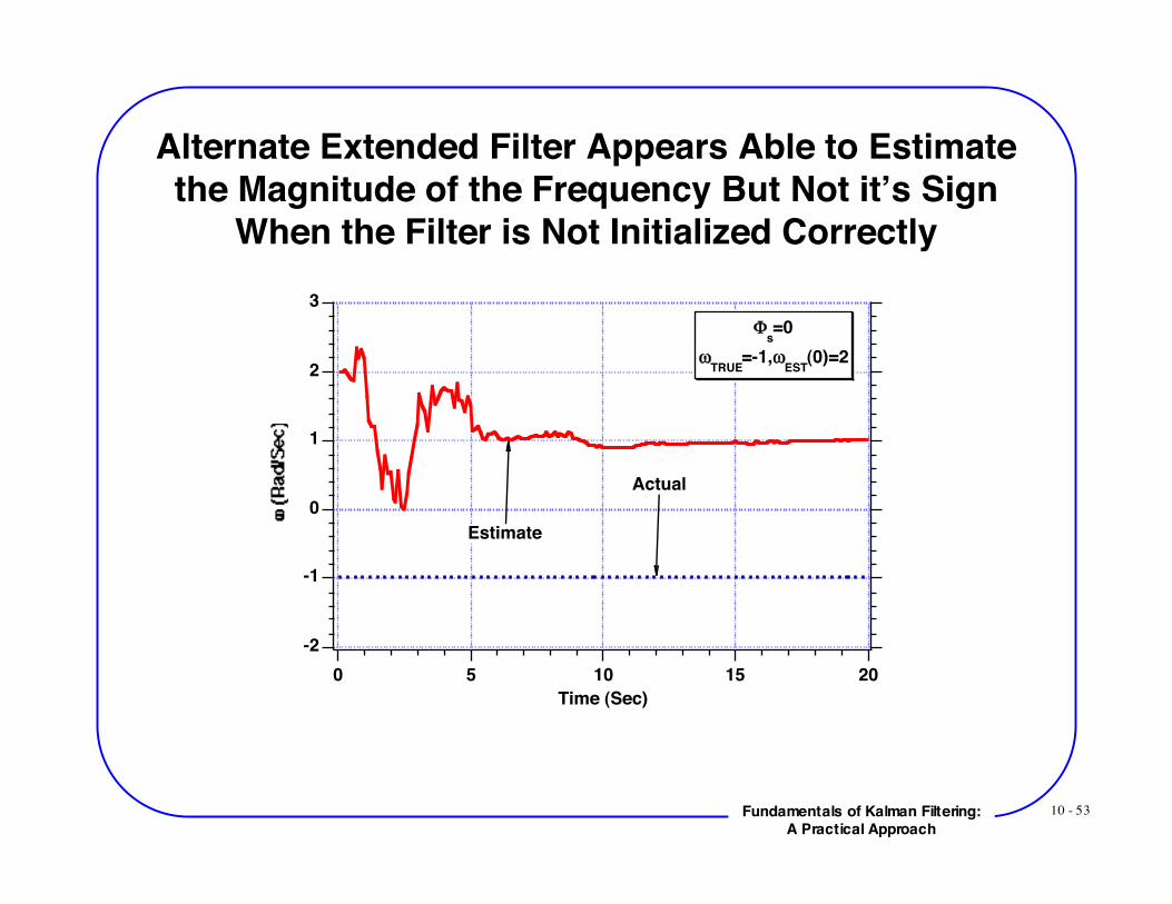
Alternate Extended Filter Appears Able to Estimatethe Magnitude of the Frequency But Not it’s Sign
When the Filter is Not Initialized Correctly3
2
1
0
-1
-220151050
Time (Sec)
Φs=0
ωTRUE
=-1,ωEST
(0)=2
Actual
Estimate
10 - 54Fundamentals of Kalman Filtering:A Practical Approach
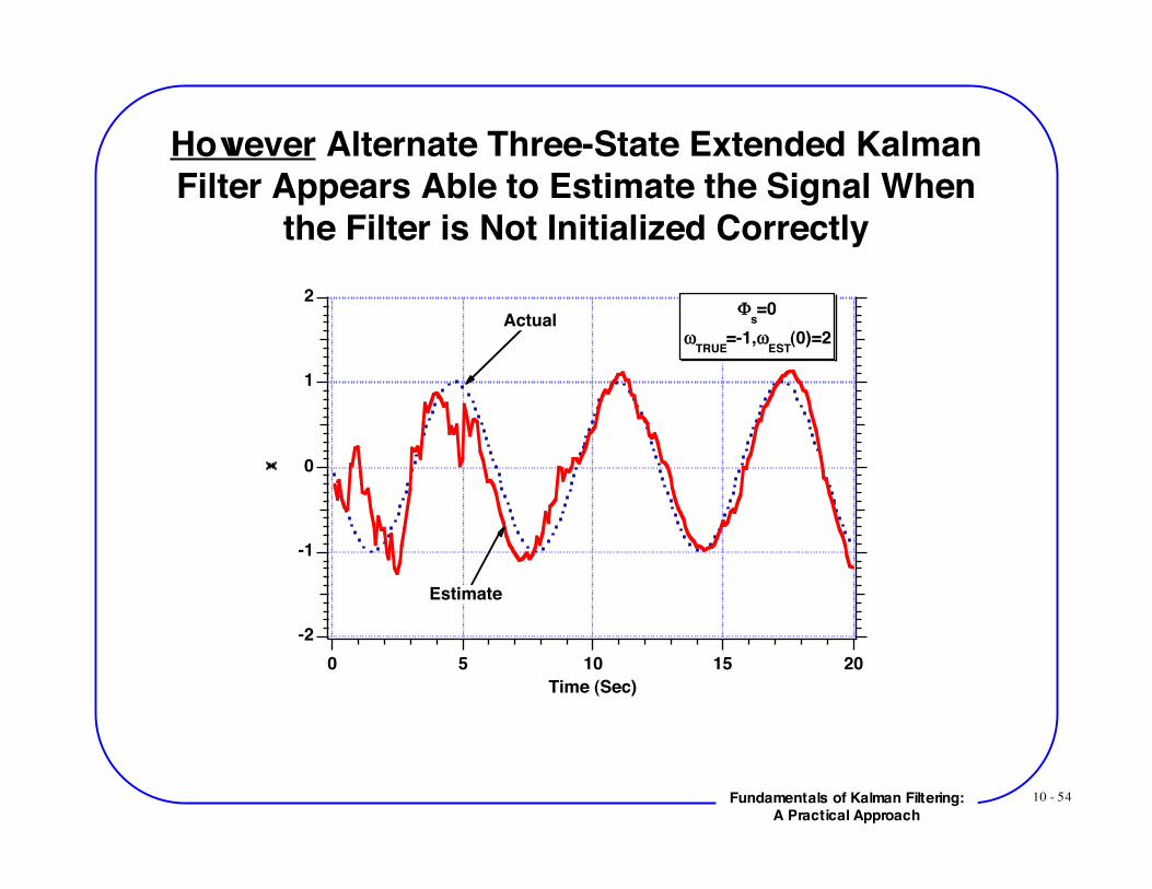
However Alternate Three-State Extended KalmanFilter Appears Able to Estimate the Signal When
the Filter is Not Initialized Correctly
-2
-1
0
1
2
20151050
Time (Sec)
!s=0
"TRUE
=-1,"EST
(0)=2Actual
Estimate
10 - 55Fundamentals of Kalman Filtering:A Practical Approach
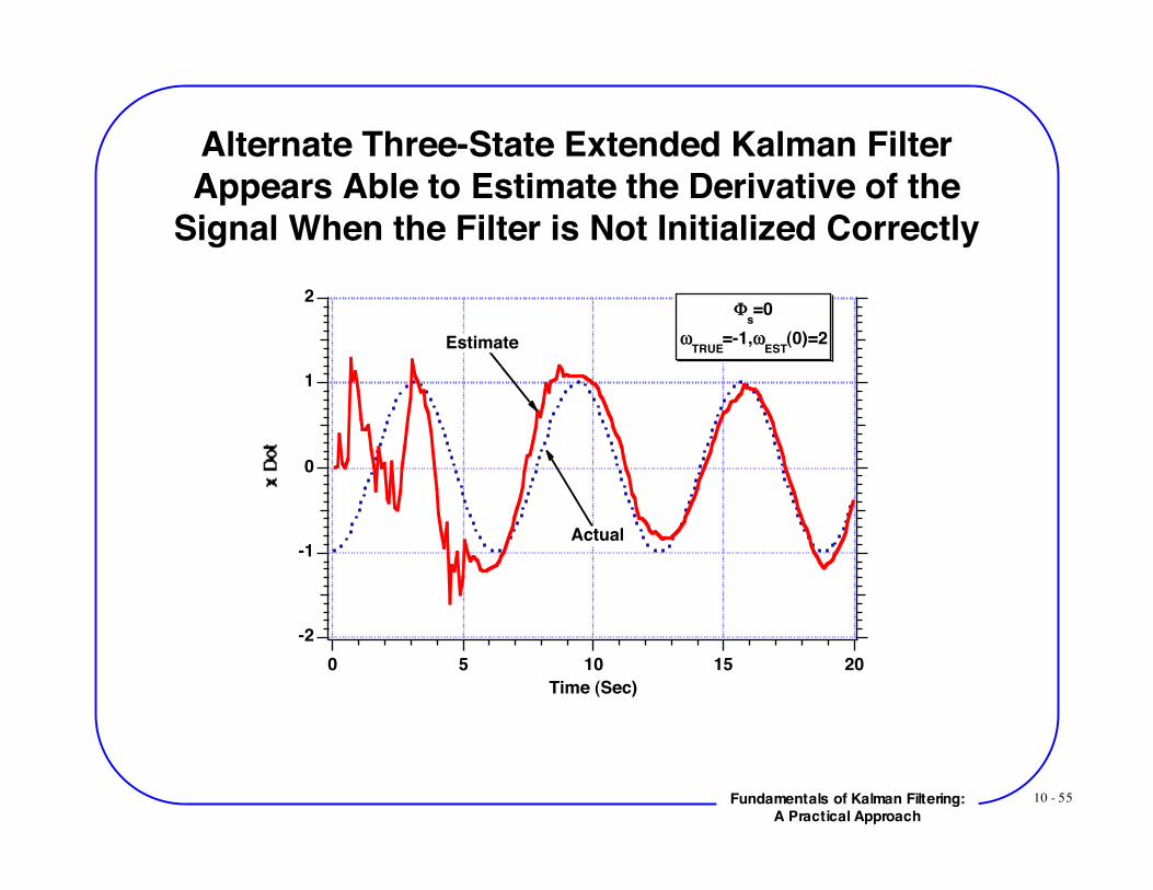
Alternate Three-State Extended Kalman FilterAppears Able to Estimate the Derivative of the
Signal When the Filter is Not Initialized Correctly
-2
-1
0
1
2
20151050
Time (Sec)
!s=0
"TRUE
=-1,"EST
(0)=2
Actual
Estimate
10 - 56Fundamentals of Kalman Filtering:A Practical Approach
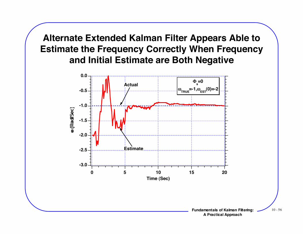
Alternate Extended Kalman Filter Appears Able toEstimate the Frequency Correctly When Frequency
and Initial Estimate are Both Negative
-3.0
-2.5
-2.0
-1.5
-1.0
-0.5
0.0
20151050Time (Sec)
Φs=0
ωTRUE
=-1,ωEST
(0)=-2Actual
Estimate
10 - 57Fundamentals of Kalman Filtering:A Practical Approach
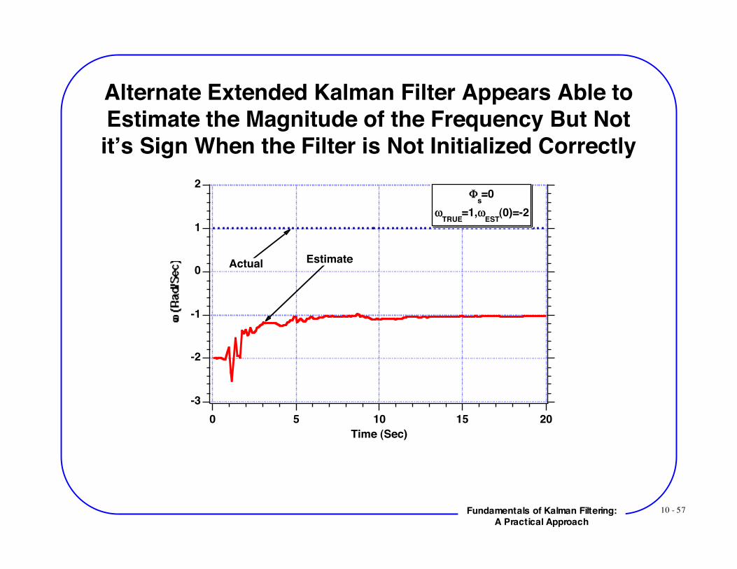
Alternate Extended Kalman Filter Appears Able toEstimate the Magnitude of the Frequency But Notit’s Sign When the Filter is Not Initialized Correctly
-3
-2
-1
0
1
2
20151050Time (Sec)
Φs=0
ωTRUE
=1,ωEST
(0)=-2
EstimateActual
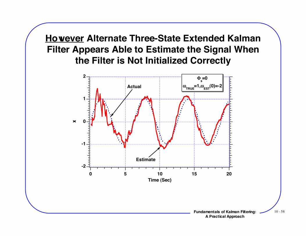
10 - 58Fundamentals of Kalman Filtering:A Practical Approach
However Alternate Three-State Extended KalmanFilter Appears Able to Estimate the Signal When
the Filter is Not Initialized Correctly
-2
-1
0
1
2
20151050
Time (Sec)
!s=0
"TRUE
=1,"EST
(0)=-2Actual
Estimate
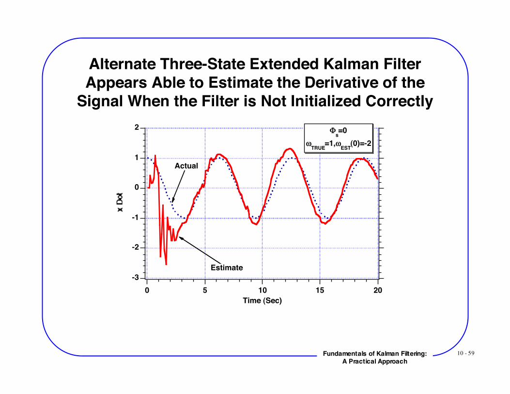
10 - 59Fundamentals of Kalman Filtering:A Practical Approach
Alternate Three-State Extended Kalman FilterAppears Able to Estimate the Derivative of the
Signal When the Filter is Not Initialized Correctly
-3
-2
-1
0
1
2
20151050
Time (Sec)
!s=0
"TRUE
=1,"EST
(0)=-2
Actual
Estimate
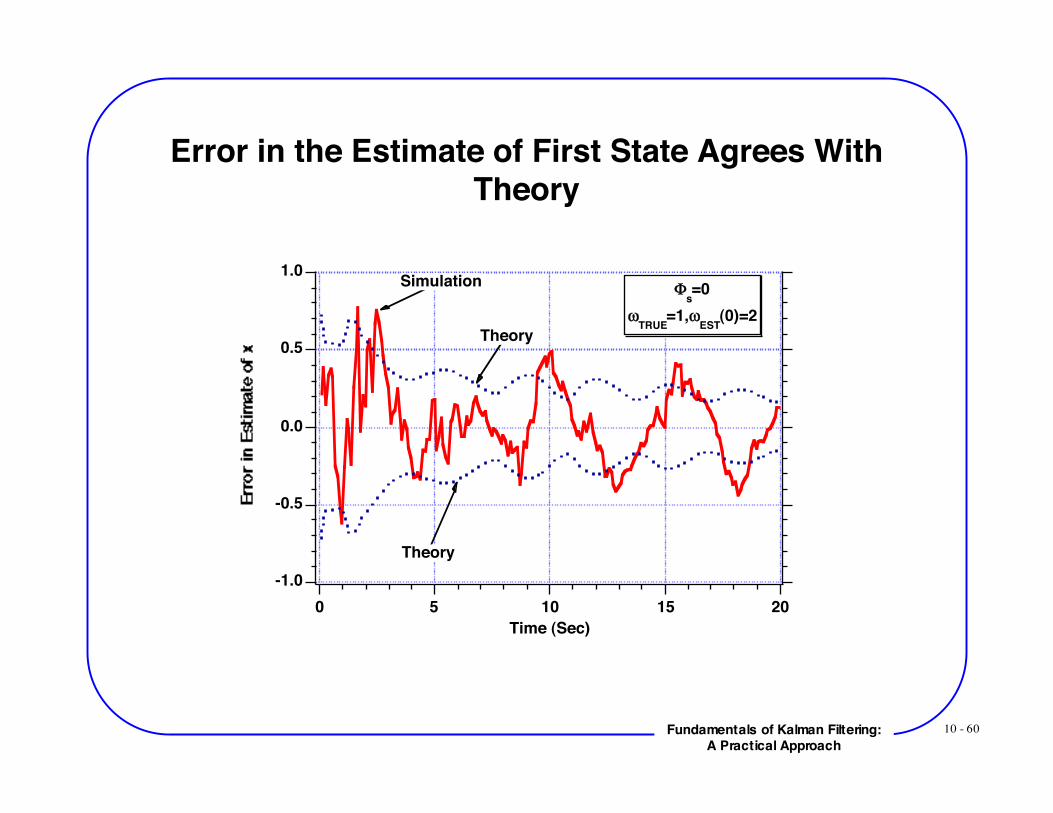
10 - 60Fundamentals of Kalman Filtering:A Practical Approach
Error in the Estimate of First State Agrees WithTheory
-1.0
-0.5
0.0
0.5
1.0
20151050
Time (Sec)
!s=0
"TRUE
=1,"EST
(0)=2
Simulation
Theory
Theory
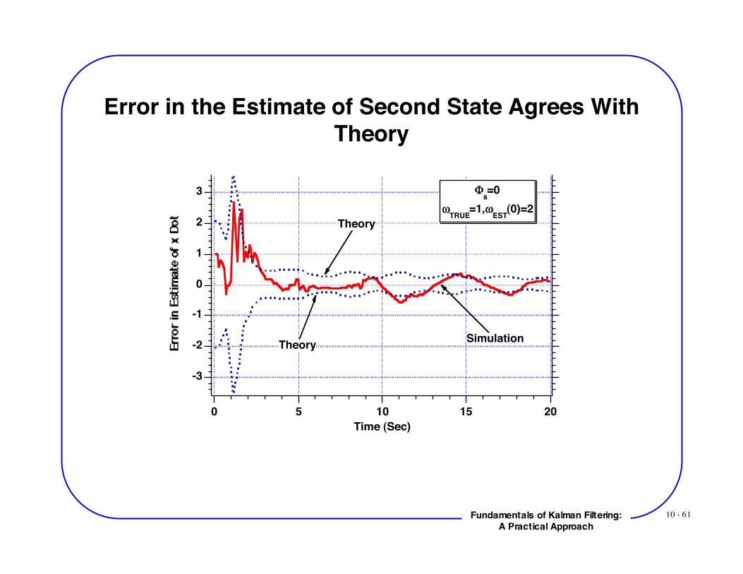
10 - 61Fundamentals of Kalman Filtering:A Practical Approach
Error in the Estimate of Second State Agrees WithTheory
-3
-2
-1
0
1
2
3
20151050
Time (Sec)
!s=0
"TRUE
=1,"EST
(0)=2
Simulation
Theory
Theory
10 - 62Fundamentals of Kalman Filtering:A Practical Approach
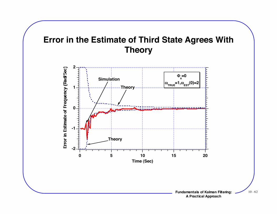
Error in the Estimate of Third State Agrees WithTheory
-2
-1
0
1
2
20151050
Time (Sec)
!s=0
"TRUE
=1,"EST
(0)=2Simulation
Theory
Theory
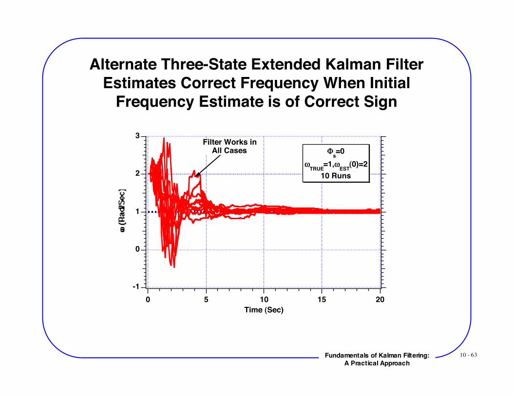
10 - 63Fundamentals of Kalman Filtering:A Practical Approach
Alternate Three-State Extended Kalman FilterEstimates Correct Frequency When Initial
Frequency Estimate is of Correct Sign
3
2
1
0
-120151050
Time (Sec)
Φs=0
ωTRUE
=1,ωEST
(0)=210 Runs
Filter Works inAll Cases
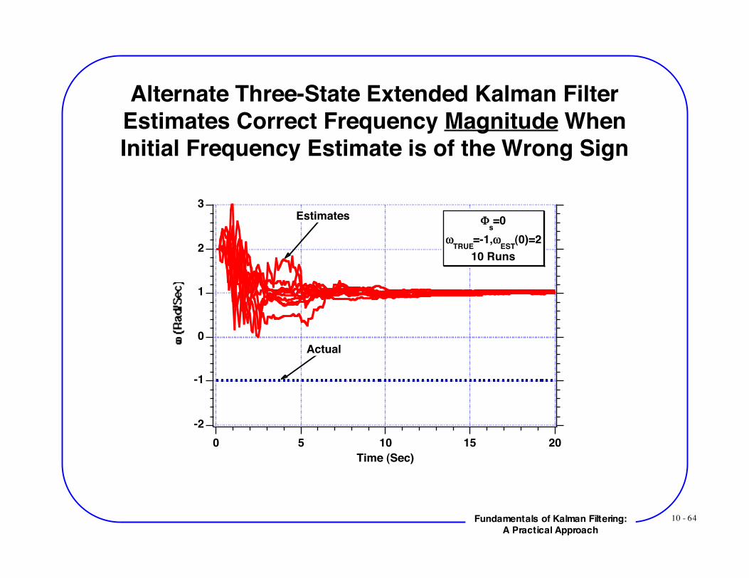
10 - 64Fundamentals of Kalman Filtering:A Practical Approach
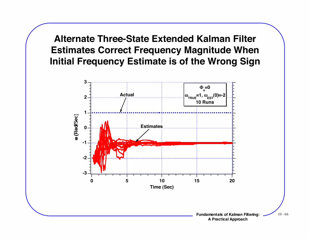
Alternate Three-State Extended Kalman FilterEstimates Correct Frequency Magnitude WhenInitial Frequency Estimate is of the Wrong Sign
3
2
1
0
-1
-220151050
Time (Sec)
Φs=0
ωTRUE
=-1,ωEST
(0)=210 Runs
Actual
Estimates
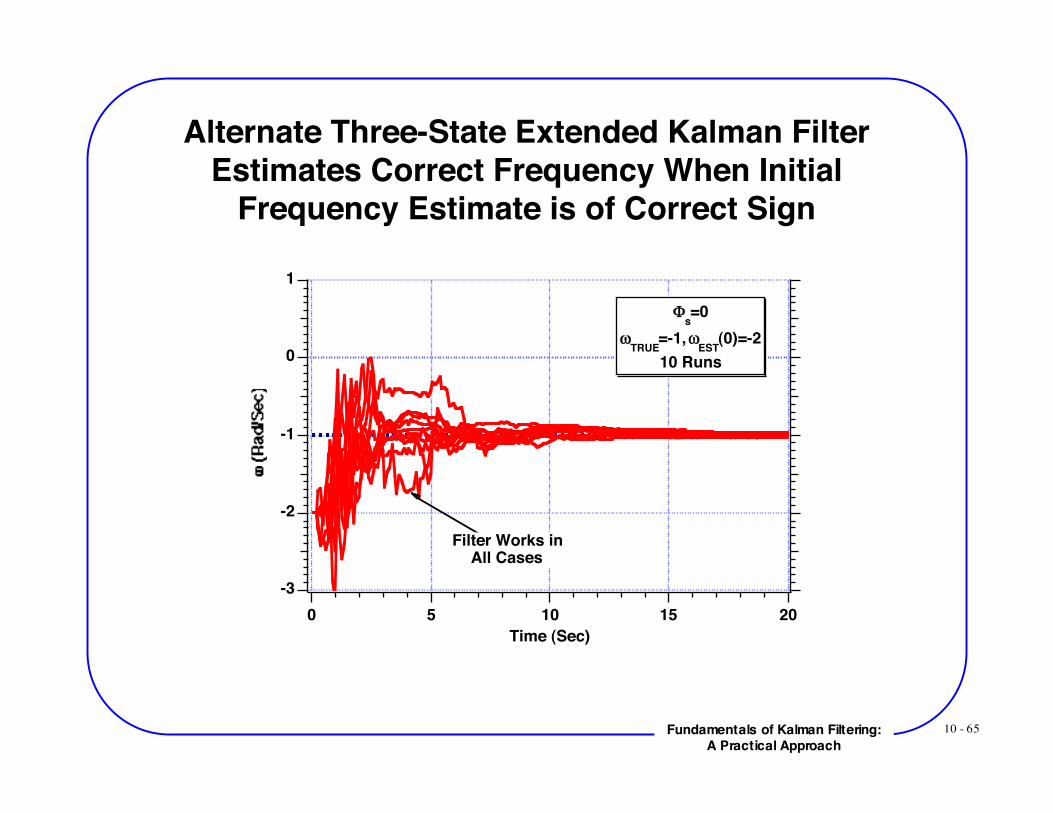
10 - 65Fundamentals of Kalman Filtering:A Practical Approach
Alternate Three-State Extended Kalman FilterEstimates Correct Frequency When Initial
Frequency Estimate is of Correct Sign
-3
-2
-1
0
1
20151050Time (Sec)
Φs=0
ωTRUE
=-1, ωEST
(0)=-210 Runs
Filter Works inAll Cases
10 - 66Fundamentals of Kalman Filtering:A Practical Approach
Alternate Three-State Extended Kalman FilterEstimates Correct Frequency Magnitude WhenInitial Frequency Estimate is of the Wrong Sign
-3
-2
-1
0
1
2
3
20151050Time (Sec)
Φs=0
ωTRUE
=1, ωEST
(0)=-210 Runs
Actual
Estimates
10 - 67Fundamentals of Kalman Filtering:A Practical Approach
Summary For Alternate Filter
• Estimate frequency when initial frequency estimate is ofsame sign as actual frequency• If initial frequency estimate is of different sign than actualfrequency we are able to estimate magnitude but not sign offrequency
- However we are able to estimate x and x dot in allcases
• Possible we can not distinguish between positive andnegative frequencies because only frequency squared termshows up in our model of the real world
x = -!2x
10 - 68Fundamentals of Kalman Filtering:A Practical Approach
Another Extended Kalman Filter For SinusoidalModel
10 - 69Fundamentals of Kalman Filtering:A Practical Approach
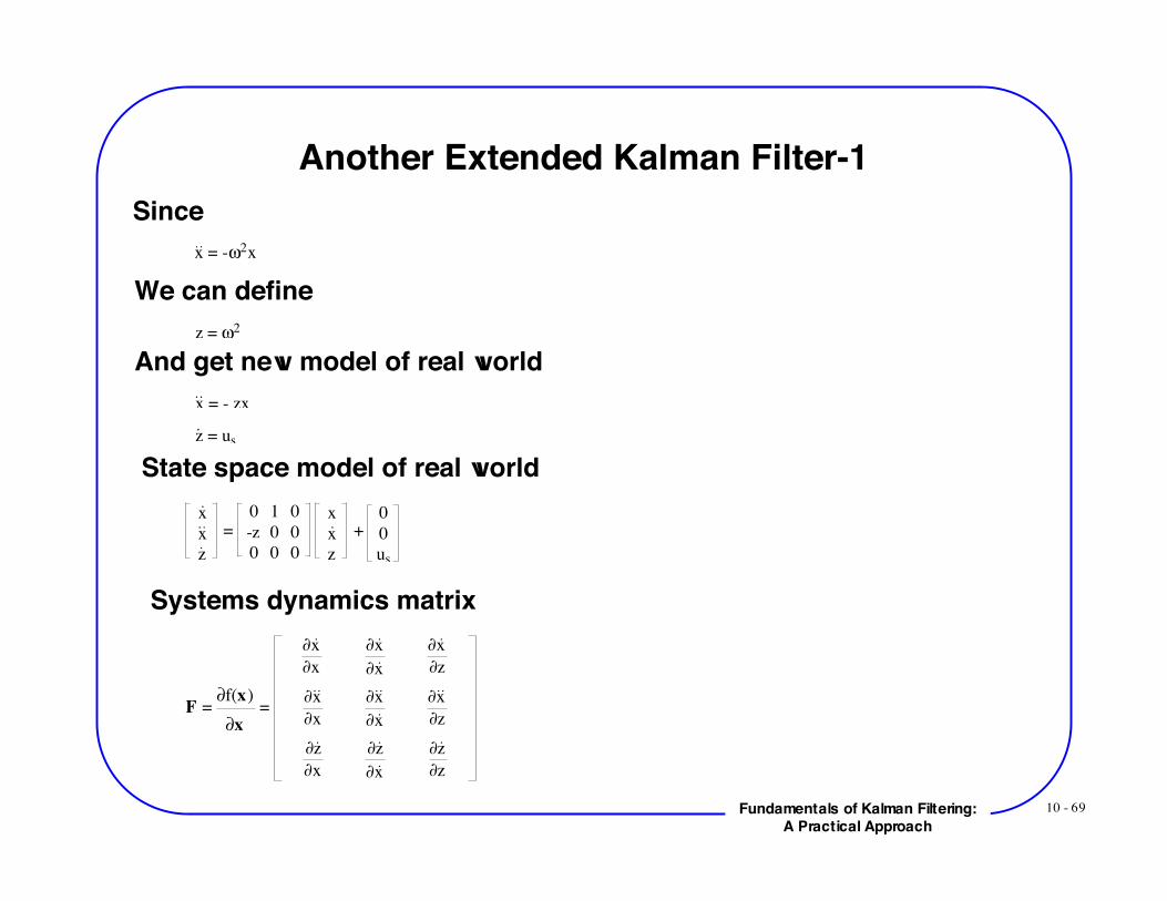
Another Extended Kalman Filter-1Since
x = -!2x
We can definez = !2
And get new model of real worldx = - zx
z = us
State space model of real worldx
x
z
=
0 1 0
-z 0 0
0 0 0
x
x
z
+
0
0
us
Systems dynamics matrix
F = !f(x)
!x
=
!x
!x
!x
!x
!x
!z
!x
!x
!x
!x
!x
!z
!z
!x
!z
!x
!z
!z
10 - 70Fundamentals of Kalman Filtering:A Practical Approach
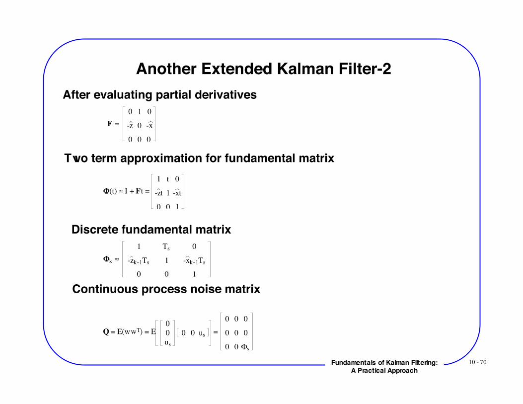
Another Extended Kalman Filter-2After evaluating partial derivatives
F =
0 1 0
-z 0 -x
0 0 0
Two term approximation for fundamental matrix
!(t) " I + Ft =
1 t 0
-zt 1 -xt
0 0 1
Discrete fundamental matrix
!k "
1 Ts 0
-zk-1Ts 1 -xk-1Ts
0 0 1
Continuous process noise matrix
Q = E(wwT) = E 0
0
us
0 0 us =
0 0 0
0 0 0
0 0 !s
10 - 71Fundamentals of Kalman Filtering:A Practical Approach
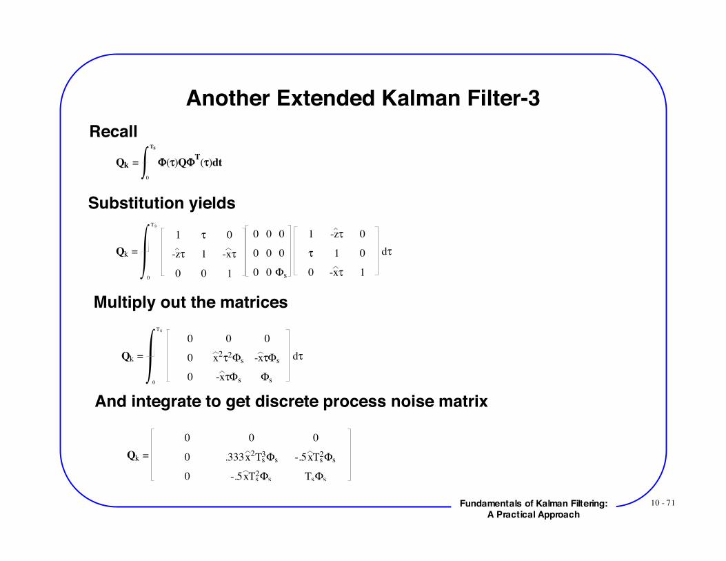
Another Extended Kalman Filter-3Recall
Qk = !(")Q!T(")dt
0
Ts
Substitution yields
Qk =
1 ! 0
-z! 1 -x!
0 0 1
0 0 0
0 0 0
0 0 "s
1 -z! 0
! 1 0
0 -x! 1
d!
0
Ts
Multiply out the matrices
Qk =
0 0 0
0 x2!2"s -x!"s
0 -x!"s "s
d!
0
Ts
And integrate to get discrete process noise matrix
Qk =
0 0 0
0 .333x2Ts
3!s -.5xTs
2!s
0 -.5xTs2!s Ts!s
10 - 72Fundamentals of Kalman Filtering:A Practical Approach
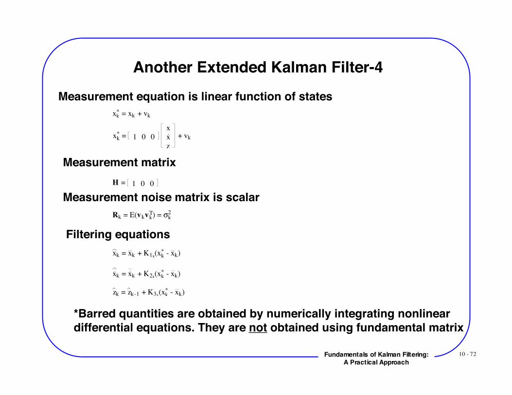
Another Extended Kalman Filter-4Measurement equation is linear function of states
xk* = xk + vk
xk* = 1 0 0
x
x
z
+ vk
Measurement matrixH = 1 0 0
Measurement noise matrix is scalarRk = E(vkvk
T) = !k2
Filtering equationsxk = xk + K1k
(xk* - xk)
xk = xk + K2k(xk
* - xk)
zk = zk-1 + K3k(xk
* - xk)
*Barred quantities are obtained by numerically integrating nonlineardifferential equations. They are not obtained using fundamental matrix
10 - 73Fundamentals of Kalman Filtering:A Practical Approach
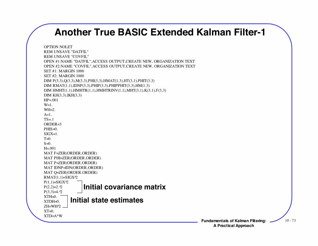
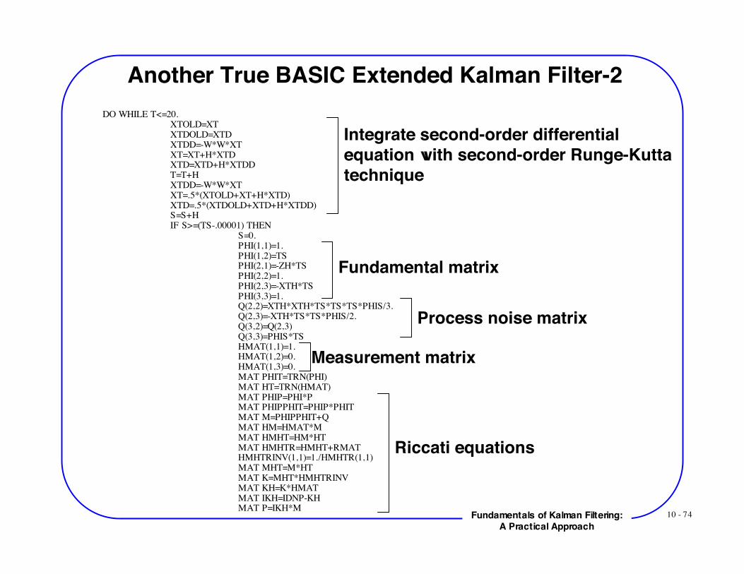
Another True BASIC Extended Kalman Filter-1OPTION NOLETREM UNSAVE "DATFIL"REM UNSAVE "COVFIL"OPEN #1:NAME "DATFIL",ACCESS OUTPUT,CREATE NEW, ORGANIZATION TEXTOPEN #2:NAME "COVFIL",ACCESS OUTPUT,CREATE NEW, ORGANIZATION TEXTSET #1: MARGIN 1000SET #2: MARGIN 1000DIM P(3,3),Q(3,3),M(3,3),PHI(3,3),HMAT(1,3),HT(3,1),PHIT(3,3)DIM RMAT(1,1),IDNP(3,3),PHIP(3,3),PHIPPHIT(3,3),HM(1,3)DIM HMHT(1,1),HMHTR(1,1),HMHTRINV(1,1),MHT(3,1),K(3,1),F(3,3)DIM KH(3,3),IKH(3,3)HP=.001W=1.WH=2.A=1.TS=.1ORDER=3PHIS=0.SIGX=1.T=0.S=0.H=.001MAT F=ZER(ORDER,ORDER)MAT PHI=ZER(ORDER,ORDER)MAT P=ZER(ORDER,ORDER)MAT IDNP=IDN(ORDER,ORDER)MAT Q=ZER(ORDER,ORDER)RMAT(1,1)=SIGX 2̂P(1,1)=SIGX 2̂P(2,2)=2. 2̂P(3,3)=4. 2̂XTH=0.XTDH=0.ZH=WH 2̂XT=0.XTD=A*W
Initial covariance matrixInitial state estimates
10 - 74Fundamentals of Kalman Filtering:A Practical Approach
Another True BASIC Extended Kalman Filter-2DO WHILE T<=20.
XTOLD=XTXTDOLD=XTDXTDD=-W*W*XT
XT=XT+H*XTD XTD=XTD+H*XTDD
T=T+HXTDD=-W*W*XT
XT=.5*(XTOLD+XT+H*XTD) XTD=.5*(XTDOLD+XTD+H*XTDD)
S=S+HIF S>=(TS-.00001) THEN
S=0.PHI(1,1)=1.PHI(1,2)=TSPHI(2,1)=-ZH*TSPHI(2,2)=1.PHI(2,3)=-XTH*TSPHI(3,3)=1.Q(2,2)=XTH*XTH*TS*TS*TS*PHIS/3.Q(2,3)=-XTH*TS*TS*PHIS/2.Q(3,2)=Q(2,3)Q(3,3)=PHIS*TSHMAT(1,1)=1.HMAT(1,2)=0.HMAT(1,3)=0.MAT PHIT=TRN(PHI)MAT HT=TRN(HMAT)MAT PHIP=PHI*PMAT PHIPPHIT=PHIP*PHITMAT M=PHIPPHIT+QMAT HM=HMAT*MMAT HMHT=HM*HTMAT HMHTR=HMHT+RMATHMHTRINV(1,1)=1./HMHTR(1,1)MAT MHT=M*HTMAT K=MHT*HMHTRINVMAT KH=K*HMATMAT IKH=IDNP-KHMAT P=IKH*M
Integrate second-order differentialequation with second-order Runge-Kuttatechnique
Fundamental matrix
Process noise matrix
Measurement matrix
Riccati equations
10 - 75Fundamentals of Kalman Filtering:A Practical Approach
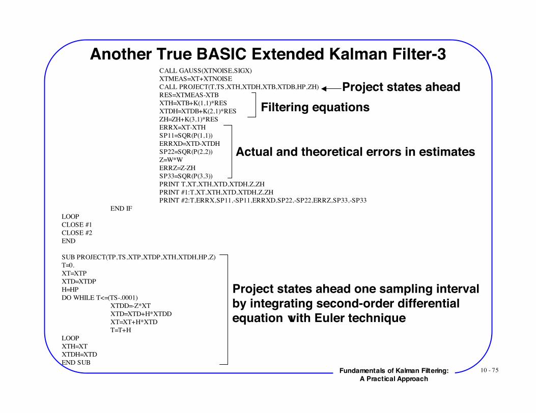
Another True BASIC Extended Kalman Filter-3CALL GAUSS(XTNOISE,SIGX)XTMEAS=XT+XTNOISECALL PROJECT(T,TS,XTH,XTDH,XTB,XTDB,HP,ZH)RES=XTMEAS-XTBXTH=XTB+K(1,1)*RESXTDH=XTDB+K(2,1)*RESZH=ZH+K(3,1)*RESERRX=XT-XTHSP11=SQR(P(1,1))ERRXD=XTD-XTDHSP22=SQR(P(2,2))Z=W*WERRZ=Z-ZHSP33=SQR(P(3,3))PRINT T,XT,XTH,XTD,XTDH,Z,ZHPRINT #1:T,XT,XTH,XTD,XTDH,Z,ZHPRINT #2:T,ERRX,SP11,-SP11,ERRXD,SP22,-SP22,ERRZ,SP33,-SP33
END IFLOOPCLOSE #1CLOSE #2END
SUB PROJECT(TP,TS,XTP,XTDP,XTH,XTDH,HP,Z)T=0.XT=XTPXTD=XTDPH=HPDO WHILE T<=(TS-.0001)
XTDD=-Z*XTXTD=XTD+H*XTDDXT=XT+H*XTDT=T+H
LOOPXTH=XTXTDH=XTDEND SUB
Project states aheadFiltering equations
Actual and theoretical errors in estimates
Project states ahead one sampling intervalby integrating second-order differentialequation with Euler technique
10 - 76Fundamentals of Kalman Filtering:A Practical Approach
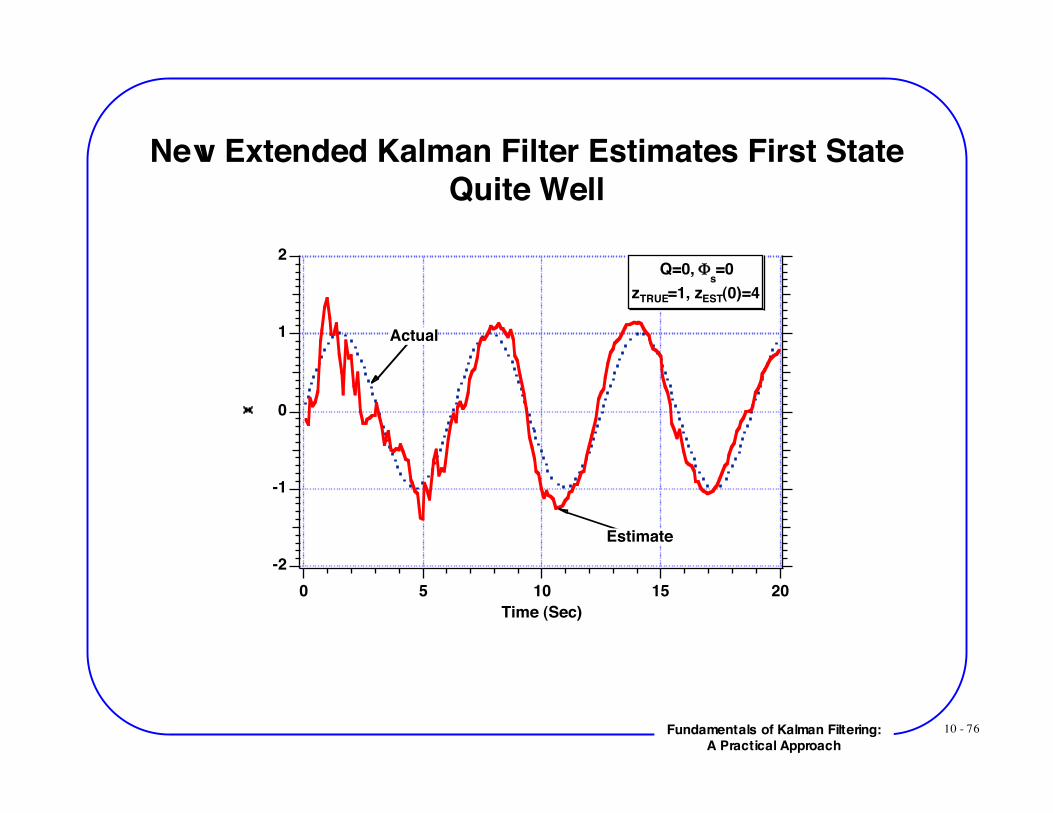
New Extended Kalman Filter Estimates First StateQuite Well
-2
-1
0
1
2
20151050
Time (Sec)
Actual
Estimate
Q=0, !s=0
zTRUE=1, zEST(0)=4
10 - 77Fundamentals of Kalman Filtering:A Practical Approach
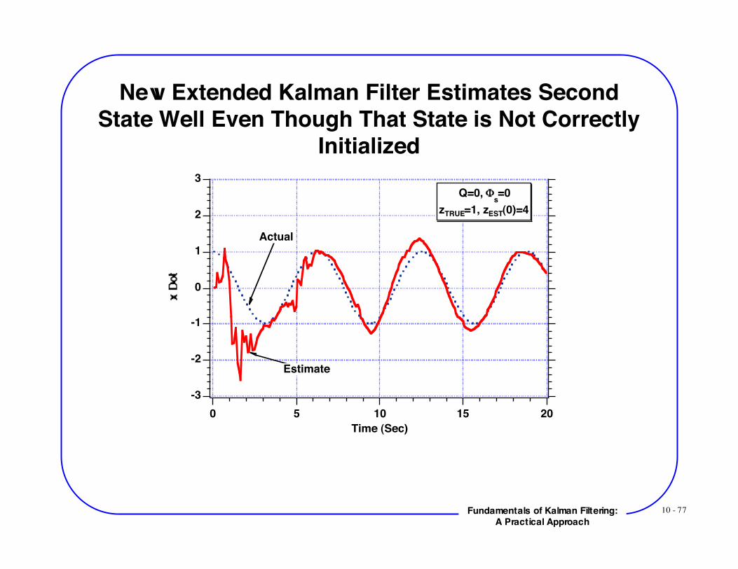
New Extended Kalman Filter Estimates SecondState Well Even Though That State is Not Correctly
Initialized
-3
-2
-1
0
1
2
3
20151050
Time (Sec)
Actual
Estimate
Q=0, !s=0
zTRUE=1, zEST(0)=4
10 - 78Fundamentals of Kalman Filtering:A Practical Approach
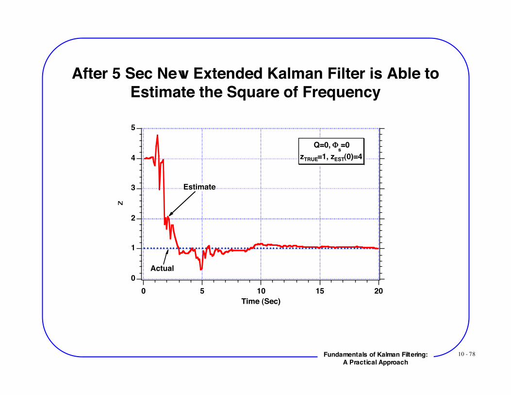
After 5 Sec New Extended Kalman Filter is Able toEstimate the Square of Frequency
5
4
3
2
1
0
20151050
Time (Sec)
Actual
Estimate
Q=0, !s=0
zTRUE=1, zEST(0)=4
10 - 79Fundamentals of Kalman Filtering:A Practical Approach
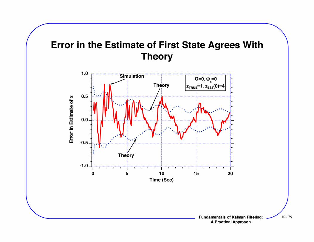
Error in the Estimate of First State Agrees WithTheory
-1.0
-0.5
0.0
0.5
1.0
20151050
Time (Sec)
Q=0, !s=0
zTRUE=1, zEST(0)=4
Simulation
Theory
Theory
10 - 80Fundamentals of Kalman Filtering:A Practical Approach
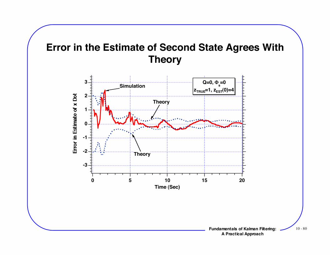
Error in the Estimate of Second State Agrees WithTheory
-3
-2
-1
0
1
2
3
20151050
Time (Sec)
Q=0, !s=0
zTRUE=1, zEST(0)=4Simulation
Theory
Theory
10 - 81Fundamentals of Kalman Filtering:A Practical Approach
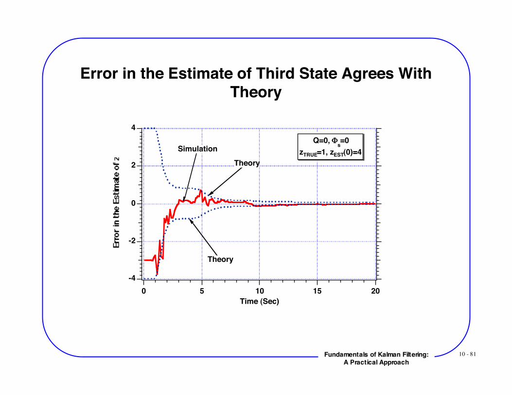
Error in the Estimate of Third State Agrees WithTheory
-4
-2
0
2
4
20151050
Time (Sec)
Q=0, !s=0
zTRUE=1, zEST(0)=4Simulation
Theory
Theory
10 - 82Fundamentals of Kalman Filtering:A Practical Approach
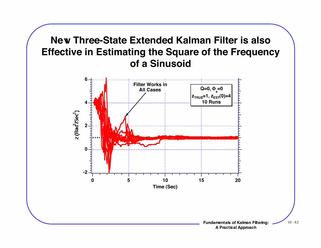
New Three-State Extended Kalman Filter is alsoEffective in Estimating the Square of the Frequency
of a Sinusoid6
4
2
0
-220151050
Time (Sec)
Q=0, Φs=0
zTRUE=1, zEST(0)=410 Runs
Filter Works inAll Cases
10 - 83Fundamentals of Kalman Filtering:A Practical Approach
Tracking a Sine WaveSummary
• Arbitrarily choosing states for filter does not guarantee thatit will work if programmed correctly• Various extended Kalman filters designed to highlight issues
- Initialization experiments were used to illustraterobustness of various filter designs