Trabajo de Iniciaci´on a la Investigaci´on: Study and … · 2 Methodology In this chapter, the...
81
Trabajo de Iniciaci´on a la Investigaci´on: Study and application of central pattern generator circuits to the control of a modular robot FernandoHerreroCarr´on Escuela Polit´ ecnica Superior, Universidad Aut´onoma de Madrid August 30, 2007
Transcript of Trabajo de Iniciaci´on a la Investigaci´on: Study and … · 2 Methodology In this chapter, the...

Trabajo de Iniciacion a la Investigacion:
Study and application of central pattern generator
circuits to the control of a modular robot
Fernando Herrero CarronEscuela Politecnica Superior, Universidad Autonoma de Madrid
August 30, 2007

2

Contents
1 Introduction 5
2 Methodology 7
2.1 CPGs to control robotic locomotion . . . . . . . . . . . . . . . . . . . . . . 72.2 Network models . . . . . . . . . . . . . . . . . . . . . . . . . . . . . . . . . 8
2.2.1 Neuron model . . . . . . . . . . . . . . . . . . . . . . . . . . . . . . 82.2.2 Synapse model . . . . . . . . . . . . . . . . . . . . . . . . . . . . . 92.2.3 Connecting neurons and synapses . . . . . . . . . . . . . . . . . . . 11
2.3 The robot . . . . . . . . . . . . . . . . . . . . . . . . . . . . . . . . . . . . 122.3.1 Control of one module . . . . . . . . . . . . . . . . . . . . . . . . . 12
2.4 CPG evaluation . . . . . . . . . . . . . . . . . . . . . . . . . . . . . . . . . 142.4.1 Simulator . . . . . . . . . . . . . . . . . . . . . . . . . . . . . . . . 172.4.2 Initial conditions . . . . . . . . . . . . . . . . . . . . . . . . . . . . 172.4.3 Diagrams . . . . . . . . . . . . . . . . . . . . . . . . . . . . . . . . 172.4.4 Phase difference and period analysis . . . . . . . . . . . . . . . . . . 18
2.5 Simulating networks of neurons . . . . . . . . . . . . . . . . . . . . . . . . 202.5.1 Advantages of the library . . . . . . . . . . . . . . . . . . . . . . . 202.5.2 Implementation . . . . . . . . . . . . . . . . . . . . . . . . . . . . . 212.5.3 Wrapping rather than inheriting . . . . . . . . . . . . . . . . . . . . 212.5.4 The constructor parameters problem . . . . . . . . . . . . . . . . . 22
3 Intermodule coordination 25
3.1 Uncoupled modules . . . . . . . . . . . . . . . . . . . . . . . . . . . . . . . 253.1.1 Motivation . . . . . . . . . . . . . . . . . . . . . . . . . . . . . . . . 253.1.2 Parameters . . . . . . . . . . . . . . . . . . . . . . . . . . . . . . . 26
3.2 Symmetrical inhibition, weak coupling . . . . . . . . . . . . . . . . . . . . 283.2.1 Motivation . . . . . . . . . . . . . . . . . . . . . . . . . . . . . . . . 283.2.2 Diagram . . . . . . . . . . . . . . . . . . . . . . . . . . . . . . . . . 283.2.3 Parameters . . . . . . . . . . . . . . . . . . . . . . . . . . . . . . . 283.2.4 Evaluation . . . . . . . . . . . . . . . . . . . . . . . . . . . . . . . . 29
3.3 Symmetrical inhibition with strong coupling . . . . . . . . . . . . . . . . . 323.3.1 Irregular activity . . . . . . . . . . . . . . . . . . . . . . . . . . . . 323.3.2 Parity synchronization mode 1 . . . . . . . . . . . . . . . . . . . . . 32
3

CONTENTS
3.3.3 Parity synchronization mode 2 . . . . . . . . . . . . . . . . . . . . . 333.3.4 Evaluation . . . . . . . . . . . . . . . . . . . . . . . . . . . . . . . . 34
3.4 Inhibitory loop . . . . . . . . . . . . . . . . . . . . . . . . . . . . . . . . . 423.4.1 Motivation . . . . . . . . . . . . . . . . . . . . . . . . . . . . . . . . 423.4.2 Parameters . . . . . . . . . . . . . . . . . . . . . . . . . . . . . . . 423.4.3 Evaluation . . . . . . . . . . . . . . . . . . . . . . . . . . . . . . . . 43
3.5 Push-pull model . . . . . . . . . . . . . . . . . . . . . . . . . . . . . . . . . 513.5.1 Motivation . . . . . . . . . . . . . . . . . . . . . . . . . . . . . . . . 513.5.2 Parameters . . . . . . . . . . . . . . . . . . . . . . . . . . . . . . . 513.5.3 Evaluation . . . . . . . . . . . . . . . . . . . . . . . . . . . . . . . . 51
3.6 Bistable intermediate neurons . . . . . . . . . . . . . . . . . . . . . . . . . 553.6.1 Motivation . . . . . . . . . . . . . . . . . . . . . . . . . . . . . . . . 553.6.2 The bistable neuron model with instantaneous state transtition . . 563.6.3 The bistable neuron model with delayed state transition . . . . . . 583.6.4 Counteracting border effects . . . . . . . . . . . . . . . . . . . . . . 593.6.5 Evaluation . . . . . . . . . . . . . . . . . . . . . . . . . . . . . . . . 60
4 Discussion 63
4.1 CPG summary . . . . . . . . . . . . . . . . . . . . . . . . . . . . . . . . . 634.1.1 Features . . . . . . . . . . . . . . . . . . . . . . . . . . . . . . . . . 654.1.2 Complexity . . . . . . . . . . . . . . . . . . . . . . . . . . . . . . . 65
4.2 Symmetry . . . . . . . . . . . . . . . . . . . . . . . . . . . . . . . . . . . . 664.3 Coupling strength . . . . . . . . . . . . . . . . . . . . . . . . . . . . . . . . 664.4 Coupling sign . . . . . . . . . . . . . . . . . . . . . . . . . . . . . . . . . . 674.5 Topology . . . . . . . . . . . . . . . . . . . . . . . . . . . . . . . . . . . . . 67
5 Future work 69
A A C++ library for simulation of dynamical networks 71
A.1 Using synapses . . . . . . . . . . . . . . . . . . . . . . . . . . . . . . . . . 72A.2 Simulating iterated maps . . . . . . . . . . . . . . . . . . . . . . . . . . . . 73A.3 Adding new models . . . . . . . . . . . . . . . . . . . . . . . . . . . . . . . 74A.4 Available wrappers . . . . . . . . . . . . . . . . . . . . . . . . . . . . . . . 75
A.4.1 SystemWrapper . . . . . . . . . . . . . . . . . . . . . . . . . . . . . 75A.4.2 IntegratedSystemWrapper . . . . . . . . . . . . . . . . . . . . . . . 75A.4.3 TimeWrapper . . . . . . . . . . . . . . . . . . . . . . . . . . . . . . 76A.4.4 SerializableWrapper . . . . . . . . . . . . . . . . . . . . . . . . . . . 77
4

1
Introduction
Locomotion is an ability inherent to the animal kingdom. Throughout evolution, alldifferent species have diversified and adapted the functions and shapes of their motororgans. This has unavoidably lead to a great variability in motor control neural systems[1]. However, despite the large number of solutions nature has come up with for the manyspecies, their study reveals common principles, for which reason knowledge about inferiorspecies can be carried to higher ones.
One characteristic common to every species is a hierarchical organization of the motorsystem. From the more cognitive tasks like the animal’s will to move, the selection ofa concrete movement and the planning of a sequence of actions, to the activation of amuscle, a number of independent functional modules coordinate to generate a coherent andeffective activity pattern. So, for instance, the movement of a limb implies a coordinationmechanism for the whole organ and delegation in control subsystems for each segment.
The goal of locomotion is to displace the animal in its environment. Therefore sensoryinput is fundamental for an effective adaptation. The locomotion system can be de-scribed as a closed loop control system [2], in which actions must always comply with theframe imposed by external conditions [3]. Experimental isolation of the sensory systemand the motor system provides us with evidence that certain activities suffer importantdegradation, to the point of completely disappearing in the absence of feedback [1]. Theimportance of understanding the role of sensory activity in the generation of movementis therefore crucial.
Nevertheless, there exist certain components that survive despite absence of this feed-back. Rhythmic movements generated by central pattern generators (CPGs) are an ex-ample.
CPGs are neural circuits that autonomously generate rhythmic activity to control mo-tor neurons and are involved in plenty of the exercises that require periodicity, robustnessand/or precision. In them, neurons activate at different phases of the rhythmic cycle. Themain characteristics of rhythms generated by this kind of circuits are stability, flexibilityand robustness [4].
Mechanisms giving rise to rhythmic activity are manifold: on one hand, the sort ofactivity of each neuron (regular spiking, bursting, chaotic bursting, etc.), and on the other
5

1. INTRODUCTION
hand the interconnection among them [5, 6]. Topology’s role is fundamental to achievethis coordination of the different components in the network. Depending on connectivityparameters, such phenomena can appear as frequency locking, phase or antiphase lockingor rhythm regularization. Through adequate connectivity, neurons with regular activ-ity can also be made to originate collective chaotic activity [7], or irregular neurons tocollectively display a richer and more stable activity than otherwise [8].
There exists evidence that justifies the existence of excitatory and inhibitory synapses.Apparently, inhibitory synapses enable the aforementioned types of coordination [8, 9, 10].
The classical approach to robot control is to model the cynematics of the robot andthen design a controller to especifically act upon its joints [11]. This implies taking intoaccount all the possible situations that the robot may encounter and program them in.Thus, the robot’s behaviour is constrained by design.
On the other hand, nature itself displays a huge range of behaviour, even in previouslyunseen environments. CPGs may not be designed with every possible input in mind, yettheir flexibility allows for different emergent responses.
In this respect chaotic activity is a very important asset. Surprisingly, rich dynamicslike those displayed by chaotic neurons allows for a larger portion of the state space ofthe system to be searched, and is a key element in finding optimal solutions [12]. That aneuron can exhibit chaotic activity does not necessarily mean that its routine behaviour beirregular. In fact, chaos usually only appears under certain combinations of parameters.
Based on these investigations, I study the use of GPGs to control and coordinate therobot described in [13]. It is a modular robot, very suitable for this work because of itsworm like behaviour. Modularity is a key principle, in which a neuronal control modelfits perfectly.
The goal of this work is to explore different configurations of CPGs that could drivethis modular worm in a stable and regular manner, to extract common principles fromthem and determine what properties (invariants) must be present for a given configurationto be a good controller.
6

2
Methodology
In this chapter, the methodology of the work is described. We begin with a short moti-vation for the use of CPGs in robotic control, including a review of their main properties.Next, the mathematical models of neurons and synapses used to implement these CPGsare presented. Following this, we explain the methods used to evaluate each CPG, andthe diagrams presented in the next chapter. To conclude, we describe the software librarythat has been created, used in all experiments.
2.1 CPGs to control robotic locomotion
Robots cover a wide range of applications: car assembling, assisted surgery, defense,entertainment... The main common characteristic is: they move in an automated manner.What sets robots appart from other “moving” machines? A car is not a robot because itmust be directly controlled be a human, so it is not just movement that defines robots,but automated control of movement.
Again, depending on application field, the requirements of this control can be diverse.In very constrained settings like assembly lines, a simple sequence of fixed targets will do,but other environments may be more demanding.
Unpredictability in these requirements is a major problem when designing robots:unpredictable goals and unpredictable perturbations must be taken into account. But itis a problem that nature has already solved.
Central Pattern Generators (CPGs) are circuits of neurons that drive muscle activity(through specific neurons called “motoneurons”) [1], and are very good candidates forautomated movement control under these uncertain conditions. When working freely theyare able to generate a stable activity (depending on design it can be regular or irregular),and they can recover from perturbations due to its attractive nature. Of course CPGsmust be specially designed for a specific target.
There are already some works applying neuroscientific knowledge to robotic control( [14, 15, 16, 17], to name a few). All of them are concerned with the generation andcoordination of various cyclic movements, e.g., legs in walking robots and modules in
7

2. METHODOLOGY
lamprey or worm robots. The approach is to couple a nonlinear oscillator to each oneof these parts and include some term in the oscillators’ equations to simulate synapticconnections.
These systems are very stable and robust because of the attracting nature of theoscillators. However, while this is a very interesting approach, it is very simplistic. Byusing systems with rich dynamics like bursting neurons and diffusion synapses we augmentthe circuit’s information capacity. We plan to take advantage of this by implementingsensory feedback into the robot in a future work.
2.2 Network models
Usually models of neurons are a mathematical description of their physical properties.Making use of differential equations, one can describe the dynamics of ion conductances,of membrane potential and any other aspect subject to change with time [18].
Since solving these differential equations is usually not feasible, one has to resort tosimulating a solution through integration algorithms. They are usually computationallycostly because they imply speculating about possible future states of the system, evalu-ating the equations many times and interpolating the speculated results.
Map models make a more phenomenological description of neurons [19, 20]. Theirpurpose is to mimic neurons’ behaviour without necessarily giving an explanation of whyor how this behaviour happens.
They can be considered as “discretized time” differential equations. Eventhough stillhard to solve and in most cases they do not have an analytical solution, the next state canbe exactly computed given the current one, as opposed to continuous differential equa-tions. Discrete maps are of the form: xn+1 = f(xn), so computing the next state involvesevaluating f only once, much more efficient than continuous integration algorithms.
2.2.1 Neuron model
All neurons of the CPGs used in this study are based on Rulkov’s model [21]. Rulkov’smodel was chosen because of its simplicity and the rich set of possible behaviours depend-ing on the selection of parameters. The mathematical description of this model is shownin equations 2.1, 2.2 and 2.3.
f(x, y) =
α1−x
+ y if x ≤ 0
α + y if 0 ≤ x < α + y−1 otherwise
(2.1)
xn+1 = f(xn, yn + βeIn) (2.2)
yn+1 = yn − µ(xn + 1) + µσ + µσeIn (2.3)
This is a bidimensional model, where variable xn represents a neuron’s membranevoltage and yn is a slow dynamics variable with no direct biological meaning, but with
8

2.2. NETWORK MODELS
similar meaning as gating variables in biological models that represent the fraction of openion-channels in the cell. So to speak, while xn oscillates on a fast time scale, representingindividual spikes of the neuron, yn keeps track of where in time the burst finds itself, asort of context memory.
Two parameters, σ and α select the working regime of the model: silent, tonic spikingor tonic bursting. In the most interesting regime for this work, tonic bursting, theyfurthermore control burst duration and period, so experimenting with these should bestraightforward.
Figure 2.1 shows the effect of changing α and σ in the tonic bursting regime1. Grossomodo, α controls the burst width and σ controls interburst intervals (while also affectingthe duration of the burst).
Since this model is phenomenological, we will not be attaching units to the plots. Itshould be undertood that abscissas will represent time evolution and ordinates membranepotential.
An undesirable side effect of parameter α is the change of amplitude of the spikes asin Figure 2.1, where a change from α = 6 to α = 15 causes a change in spike amplitudefrom approximately 4 a.u. to approximately 14 a.u. Every time this parameter is changedin a network, synapses must be readjusted since the new amplitude might be larger thanthe synapse’s reversal potential. More on this in the next section.
2.2.2 Synapse model
Synaptic models are based on Destexhe’s model [22]. To sum up, they model chemi-cal synapses that release a neurotransmitter during a certain amount of time after thepresynaptic neuron has crossed a given threshold value for its membrane potential.
Equation 2.4 is the equation that defines the ratio of bound chemical receptors inthe postsynaptic neuron2, where r is the fraction of bound receptors, α and β are theforward and backward rate constants for transmitter binding and [T ] is neurotransmitterconcentration. The condition on time specifies that during ρ units of time after thepresynaptic neuron’s membrane potential last crossed3 threshold τ (moment tf ), there isa concentration [T ] of neurotransmitter in the synaptic cleft that can be bound to freereceptors in the postsynaptic neuron. After ρ units of time, there is no more release ofneurontransmitter, thus the only term affecting r is the unbounding of already boundedreceptors.
r =
{
α[T ](1 − r) − βr if tf < t < tf + ρ−βr otherwise
(2.4)
In this work we set this threshold to be at τ = 0, so that each single spike within aburst will cause neurotransmitter release at a constant concentration [T ] = 1 for ρ = 0.01
1For an explanation of all possible regimes see [21]2we will sometimes call it “synaptic activation”3such that (Vt < τ) & (Vt+dt ≥ τ)
9

2. METHODOLOGY
-8
-6
-4
-2
0
2
4
6
8
10
0 5000 10000 15000 20000
(a) α = 15, µ = 0.001, σ = −0.33, βe = 0, σe = 1
-8
-6
-4
-2
0
2
4
6
8
10
0 5000 10000 15000 20000
(b) α = 15, µ = 0.001, σ = −1, βe = 0, σe = 1
-2.5
-2
-1.5
-1
-0.5
0
0.5
1
1.5
2
2.5
0 5000 10000 15000 20000
(c) α = 6, µ = 0.001, σ = −0.33, βe = 0, σe = 1
-2.5
-2
-1.5
-1
-0.5
0
0.5
1
1.5
2
2.5
0 5000 10000 15000 20000
(d) α = 6, µ = 0.001, σ = −0.45, βe = 0, σe = 1
Figure 2.1: Effect of parameters α and σ in Rulkov’s map: for a greater value of α, bursts getlonger ((a) and (b) compared to (c) and (d)), with more spikes; for a lower value of σ, interbursttime gets longer ((b) and (d) compared to (a) and (c)). These values are restricted to a regionwhere the model shows tonic bursting; other combinations may give rise to tonic spiking, silentor chaotic behaviours.
units of time and [T ] = 0 the rest of the time.
Synaptic current is then calculated as in equation 2.5, where I(t) is synaptict currentat time t, g is synaptic conductance, r(t) is the fraction of bound receptors at time t,Vpost(t) is the postsynaptic neuron’s membrane potential and Esyn its reversal potential.It is called reversal potential because the direction of the current will change dependingon whether Vpost is greater or less than Esyn.
I(t) = g · r(t) · (Vpost(t) − Esyn) (2.5)
Esyn controls whether a synapse is excitatory or inhibitory. If Esyn is always smallerthan the postsynaptic neuron’s potential, then I(t) will always be positive, thus thesynapse is excitatory. If, on the other hand, Esyn is always greater than Vpost, it will be
10

2.2. NETWORK MODELS
inhibitory. For this reason the reversal potential of synapses must be readjusted everytime parameter α is changed in a postsynaptic neuron, since changing α also changesthe amplitude of the postsynaptic membrane potential and this may change the intendedeffect of the synapse.
2.2.3 Connecting neurons and synapses
Let’s put the two models together in a very simple network consisting of two neurons andone synapse from one to the other like shown in Figure 2.2.
N1
SN2
Figure 2.2: simple network of two neurons, one (N1) inhibiting the other (N2) through aninhibitory synapse (S).
To obtain the full equations of the network we must substitute the generic terms forthe actual ones. Let’s do it for all three “objects” of the network.
Since N1 does not have any input, we let In = 0 in 2.2 and 2.3, thus its equationsbecome:
x(1)n+1 = f(x(1)
n , y(1)n ) (2.6)
y(1)n+1 = y(1)
n − µ(x(1)n + 1) + µσ (2.7)
For S, we must substitute the time when N1 last crossed S’s threshold and the post-synaptic potential of N2: we substitute tf for n
(1)f and Vpost for x(2)
n in equations 2.4 and2.5:
r =
{
α[T ](1 − r) − βr if n(1)f < t < n
(1)f + ρ
−βr otherwise(2.8)
I(t) = g · r(t) · (x(2)n − Esyn) (2.9)
We now have quantities defined for continuous time mixed with ones defined in discretetime. We need to discretize I(t) and r(t) in order for the equations to make sense.
In order to compute I(t) and r(t), we use an algorithm of the Runge-Kutta family,which defines sequences In and rn, much like a sampling process. The algorithm takesas input a time step that specifies the time interval between sampling In and In+1. The
11

2. METHODOLOGY
shorter the interval, the more precise the approximation, but the more steps will be neededto simulate a given amount of time.
In this work, synapses are simulated ten times more often than neurons. The reasonis that using a smaller time step and higher evaluation frequency we achieve a smootherbehaviour. The equations could be finally written as:
rSn = nth integration step of the
Runge − Kutta algorithm for r (2.10)
ISn = g · rS
n · (x(2)⌊n/10⌋ − Esyn) (2.11)
To obtain the equations for N2, we must only substitute the term for the input current:
x(2)n+1 = f(x(2)
n , y(2)n + βeI
S10n) (2.12)
y(2)n+1 = y(2)
n − µ(x(2)n + 1) + µσ + µσeI
S10n (2.13)
Figures 2.3 and 2.4 show how synapse S in Figure 2.2 behaves depending on the pre-and postsynaptic neurons. Figure 2.3 shows how when N1 fires, the synapse S releasesneurotransmitters that bind to N2 receptors (higher value of r). The higher N1’s frequencyis, the higher the synaptic activation. As the figure shows, spike frequency decreases asthe burst gets closer to its end, and so does synaptic activation too. Figure 2.4 showsthe resulting inhibitory synaptic current and its effect on N2. The activation of thesynapse produces a negative current that terminates the burst earlier and causes a longerinterburst interval.
2.3 The robot
The robot for which a control system is being designed is introduced in [13]. It consistsof several modules attached one after another through special connection points. Eachof these modules consists of two triangle shaped rigid pieces, joint by one vertex of thetriangle, and a servomotor controlling the angle between these two pieces. Figure 2.5shows a diagramatic representation of the actual robot shown in Figure 2.6.
In this work, a robot of ten modules has been considered. The parity of the numberof modules may have an effect on some CPG models, but it has not been investigated.
2.3.1 Control of one module
The first goal is to establish a central pattern generator (CPG) that can drive a singlemodule. We propose a very simple circuit that generates an oscillatory activity.
The organization of the module is shown in Figure 2.7(a). There are two endoge-nously rhythmic neurons (R and P) interconnected with inhibitory synapses. The role of
12

2.3. THE ROBOT
0
0.2
0.4
0.6
0.8
1
1.2
1.4
1.6
0 5000 10000 15000 20000 25000
a.u.
n
-8
-6
-4
-2
0
2
4
6
8
10
Mem
bran
e po
tent
ial
rn
x(1)⌊n/10⌋
Figure 2.3: Presynaptic neuron membrane potential and synaptic activation in the postsynapticneuron (variable r in [22], scaled by a factor of 100). Synaptic activity closely follows neuralactivity, although there is a noticeable delay between the onset of the burst and the highestsynaptic rate value. The three different stages of synaptic activation correspond to three differentfrequencies of the presynaptic neuron. Synapse parameters: α = 0.5, β = 10, τ = 0, Esyn = 9,gsyn = 1.5, [T ]max = 1 and release time = 0.01. Neuron parameters: α = 15, µ = 0.001,βe = 0, σe = 1 and σ = −0.33.
inhibition is to prevent both neurons from firing at the same time. When one fires, theother’s activity is delayed. In turn, when the second neuron is bursting, it delays the firstneuron’s activity and the cycle begins again. After some cycles, the two neurons arriveat a steady anti-phase state. These neurons are connected to the motoneuron (M) with avery simple synapse consisting only of a threshold function (eq. 2.14).
The motor neuron integrates its input and produces a signal that directly drives themotor, according to equation 2.15, where m is the output of neuron (M), the s terms areinput from (R) and (P) and τ is a time constant that controls how quick the output signalm will change.
Due to the opposed contribution from the s term from (R) and the s term from (P)(opposite sign for the α parameter), and the fact that (P) and (R) oscillate in anti-phase,the solution m(t) is a function oscillating between −α and α. When the motoneuron
13

2. METHODOLOGY
-3
-2.5
-2
-1.5
-1
-0.5
0
0 5000 10000 15000 20000 25000
Syn
aptic
cur
ent
n
-8
-6
-4
-2
0
2
4
6
8
10
Mem
bran
e po
tent
ial
In
x(2)⌊n/10⌋
Figure 2.4: Postsynaptic neuron membrane potential and synaptic current (variable I in [22],scaled by a factor of 10). Note how, due to the effect of the inhibitory synapse, the burst isshorter and the time between bursts is larger than in the presynaptic neuron, despite havingthe same parameters. Synapse parameters: α = 0.5, β = 10, τ = 0, Esyn = 9, gsyn = 1.5,[T ]max = 1 and release time = 0.01. Neuron parameters: α = 15, µ = 0.001, βe = 0, σe = 1and σ = −0.33.
receives no input because (P) and (R) are silent, it will go back to zero due to the −mterm in eq. 2.15.
Figure 2.7(b) shows an example pattern of activity of an isolated module.
s(α,t)(x) =
{
α if x > t0 otherwise
(2.14)
τm = −m + s(α,t)(Rx) + s(−α,t)(Px) (2.15)
2.4 Central pattern generator evaluation
In this section we explain the methods used to evaluate the CPGs as well as the diagramsand plots used in the following chapter, where we discuss the different proposed CPGs
14

2.4. CPG EVALUATION
Figure 2.5: General schema of the worm robot. A single module is marked in grey, all othermodules are exactly equal to this one.
Figure 2.6: Picture of the actual robot (taken with permission fromhttp://www.iearobotics.com).
15

2. METHODOLOGY
(a)
-30-20-10
0 10 20 30
0 5000 10000 15000 20000 25000 30000 35000 40000 45000 50000
angl
e
time
M
-8-6-4-2 0 2 4 6 8
10
Px
P
-8-6-4-2 0 2 4 6 8
10
Rx
R
(b)
Figure 2.7: (a) Organization of the CPG within one module. The promotor ’P’ and remotor’R’ neurons are interconnected with inhibitory synapses so that they synchronize in anti-phase.The motoneuron ’M’ sends a command signal to the servomotor specifying the angle at which theservo should position itself. The signal generated by ’P’ is directly input to ’M’, and the oppositeof the signal generated by ’R’ is input to ’M’. ’M’ integrates its input according to equation2.15. (b)Activity sample. Neuron ’R’ contributes positively and raises M to 30; neuron ’P’ doesexactly the opposite and drives ’M’ towards -30. ’P’ and ’R’ are synchronized in anti-phase.With no input, ’M’ goes to zero. Parameters for ’P’ and ’R’: α = 15, µ = 0.001, σ = −0.33,betae = 0, σe = 1; parameters for the inhibitory synapses between ’P’ and ’R’: α = 0.5, β = 10,τ = 0, Esyn = 9, gsyn = 1.5, T = 1, release time = 0.01; Parameters for ’M’: α = 30, τ = 0.5,t = −1.5.
16

2.4. CPG EVALUATION
for the control and coordination of the robot.
2.4.1 Simulator
All models have been implemented and tested on a rigid body dynamics simulator. Theoriginal simulator was developed by Juan Gonzalez4 and Rafael Trevino and has beenadapted to support the CPGs of this work.
The simulator places a virtual modular robot in a virtual world and simulates gravity,friction and inertia with help of the ODE5 physics engine.
2.4.2 Initial conditions
At the beginning of a simulation neurons are set to a known state. For random initialconditions, every neuron is iterated a random number of times before the simulation. Thisbrings neurons into a random but steady state.
Synapses start with its ’binding rate’ variable r set to zero.
2.4.3 Diagrams
For every model CPG proposed there will be an explanatory diagram showing how mod-ules are interconnected. Except where explicitly noted, all topologies will have repetition,meaning all modules will have the same interconnection scheme. Therefore some diagramswill only show the topology for two adjacent modules. It should be understood that thesame scheme is repeated for the rest of the modules. Sometimes there is no possibility ofrepeating the whole scheme at the borders. In these cases the scheme is repeated as faras it is possible.
When diagrams are too complicated, only one side may be shown (either promotorsor remotors only). This implies that the other side has the same connectivity pattern.
Neurons
Neurons will be represented with a white circle labelled ’P’ for promotor neurons, ’R’for remotor neurons, ’B’ for “bistable” neurons and ’side’ for a regular neuron in the“inhibitory loop” CPG (both on the promotor and the remotor sides):
4http://www.iearobotics.com5http://www.ode.org
17

2. METHODOLOGY
Synapses
Synapses will be finished with a filled triangle when they are excitatory and with a filledcircle when they are inhibitory:
2.4.4 Phase difference and period analysis
In order to capture the relevant aspects of the evolution in time of a given central pat-tern generator circuit, we provide two diagrams: time evolution of intermodule phasedifferences and time evolution of bursting period.
The diagrams included are extracted from one simulation, they are not in any waythe mean behaviour, but they are chosen so that they are representative enough. Definingwhat is representative is done by direct observation of both the diagrams and behaviourin the simulator.
The length of one period is calculated as the number of iterations from the beginningof one burst to the beginning of the next one. The beginning of one burst is determined asthe moment at which a signal crosses the threshold value τ = −1.2 upwards. The Rulkovmap resets intraburst spikes to a fixed value of −1, so in a “normal” regime neuronsshould only meet this condition when initiating a burst.
It is possible that a neuron remaining in underthreshold oscillation crosses this valueof τ = −1.2, but every model was inspected for this phenomenon and it did not appearin any of the examples shown.
Phase difference diagrams
Phase difference between modules is a key aspect of sequence generation.We provide diagrams showing the time evolution of phase differences between every
three consecutive modules, taking the first neuron as the reference. As an example, Figure2.8 shows how phase differences φ1 and φ2 are calculated between N1 and N2 and N1 andN3.
Phase difference evolution is usually smooth. There are some cases when one neuronovertakes another one and this appears as a straight line crossing the diagram from 0 to 1or from 1 to 0. This is not a discontinuity, but rather an effect of the modular arithmeticproperties of phase.
Bursting period diagrams
Phase difference conveys a very meaningful information, but it might happen that whilephase difference between two neurons is maintained constant, both neurons may be equallychanging their periods. Therefore both phase difference and period informations arecomplementary.
18

2.4. CPG EVALUATION
N1
N2
N3
B1,1 B1,2 B1,3
B2,1 B2,2 B2,3
B3,1 B3,2 B3,3
d1,1 = B2,1 − B1,1
d2,1 = B3,1 − B1,1
d2,2 = B3,1 − B1,2
P1 = B1,2 − B1,1
P2 = B1,3 − B1,2
φ1,1 = d1,1
P1
φ2,1 = d2,1
P1
φ2,2 = d2,2
P2
Figure 2.8: An example of how phase differences are calculated. Bi,j represents the beginningof the j − th burst of neuron i. We take neuron N1 as the reference and measure its first period,P1. We record the times at which the other two have last fired before B1,2 and measure thedifference between those times and the beginning of the period: d1,1 and d2,1. Phase difference
between N1 and N2 is calculated as φ1,1 =d1,1
P1, and likewise φ2,1 for N1 and N3. We now take
the next burst of N1 and repeat the operation. Notice that our algorithm takes the last burst ofthe other two neurons before B1,3, which might occur in time prior to B1,2, as is the case forB3,1. In this case, our algorithm would yield a negative value for the phase difference φ2,2.
19

2. METHODOLOGY
Period diagrams are calculated in a similar manner to phase differences diagrams: forevery neuron we calculate the time tn at which the nth burst crosses the threshold valueτ = −1.2 and the next time tn+1 when the next burst crosses the threshold again. Thevalue of period pn+1 is defined as pn+1 = tn+1 − tn.
Bursting period evolution diagrams show, for a burst numbered n, how many iterationshave passed since the beginning of burst number n − 1. It is worth noting that burstnumber n of neuron p does not necessarily coincide in time with burst number n ofanother neuron p′. In fact, it is rarely so. Most of the time they will be at most one cycleapart, but it could well be the case that there is a long time between both.
The time at which a burst occurs equals the sum of all previous periods, i.e., thesummation of the area under the curve of the diagram up to the point of that burst.
2.5 Simulating networks of neurons
Neuroscience’s aim is to understand the nervous system. In this endeavour it uses toolslike electrophysiology to gather data, statistics to analyze those data, mathematics tohypothesize models and computers to test those models and make predictions.
We have created a C++ library that precisely fits in this last area. Both neurons andsynapses are usually described by a set of differential equations that, when integrated overtime, give as result a set of functions of time representing the neuron’s or the synapse’sactivity. The main goal of this library is to provide some models of neurons and synapsesand the methods to integrate them over time.
More specifically, the goals of this library are:
• Reusability: models and mathematical methods must be easily reuseable in otherprojects, relying for that on C++’s mechanisms.
• Performance: the simulation must be as fast as possible
• Modularity: there must be a clear cut between neurons, synapses, integrators andso on (so that they can be independently reused).
• Flexibility: elements must be easy to combine and connect, and their parameterseasy to change.
• Usability: the end user of the library must be able to easily construct networks ofneurons.
2.5.1 Advantages of the library
Given the complexity of the CPGs used in this work and the high number of variablesthey involve, an object-oriented library is a very helpful tool for encapsulating data andbehaviour. Using objects helps divide variables and equations that belong together inmanageable logical units that can be treated as single entities. The traditional procedural
20

2.5. SIMULATING NETWORKS OF NEURONS
approach would have all variables and equations in the same scope, which leads to a codeharder to change and understand.
The use of C++’s templates makes this library very easy to extend. End users donot need to write much code to add new models. Instead, the library provides extensionmechanisms in the form of wrappers that allow the user to have a whole family of classesjust writing one himself. This reduces redundancy of code (the end user does not need tocopy the same code over and over) and favours refactoring, since code is located in onesingle place.
As a result, it is very easy to implement CPGs comprising different models of neuronsand synapses, including simulating them and accessing their parameters and variables. Atutorial on using the library can be found in Appendix A.
2.5.2 Implementation
The library is implemented in C++ for various reasons. The language is natively com-piled, which produces very fast executable programs. Furthermore, C++ is a multi-paradigm programming language, combining several features of structured and objectoriented programming.
A very powerful feature of C++ on which this library heavily relies is parameterization.Template techniques have seen a large development over the last decades, helping indeveloping highly modular and reusable software.
From the user’s point of view, there are three main components in the library:
Models: classes specifying which variables, parameters and equations a given class ofsystems has.
Integrators: classes that calculate the values of the variables of a given system for sometime step.
Wrappers: classes that add some functionality to other classes, much like the decoratorpattern [23].
From the developer’s point of view there are other two parts, to implement the tech-nique described in [24]:
Concept checking classes: helper classes to check for parametric polymorphism inC++ templates .
Archetypes: classes that implement the basics to meet a concept’s requirements.
2.5.3 Wrapping rather than inheriting
The library uses traditional object oriented inheritance combined with parameterizationto offer a very flexible functionality extension mechanism: wrappers.
21

2. METHODOLOGY
Wrappers’ goal is to take away common code from classes implementing the neuronmodels. By using these wrappers, the end user should be able to combine the extensionshe wants, in any arbitrary order. The first idea was to use recurring template inheritance[25]. This technique proved not to be the most effective in terms of how simple modelclasses could be.
After having written this library, I found out that this technique is called mix-inprogramming in the literature. The key idea is that mixins implement functionalityextensions without knowing what is going to be extended (as opposed to plain objectoriented inheritance). The user has the freedom to combine this extensions as he wants.For a brief review of the technique, see [26]. Figure 2.9 explains wrapping.
Extension through classical inheritance is bounded to one single extended class, thusextensions must be rewritten for every class to be extended. Wrapper extensions takeadvantage of parameterization so that one extension is only written once for all extensibleclasses. It is the compiler who is then responsible for creating the actual derived classes.This approach has, however, certain drawbacks. C++ does not provide a direct method tocheck if the class to be extended meets certain interface requirements. Siek and Lumsdainepresent in [24] a technique called “concept checking” that to some extent solves theproblem.
2.5.4 The constructor parameters problem
In C++, all methods are inherited from the base class except for constructors. Thereforethe derived class’s constructor must explicitly provide the appropriate parameters to con-struct the superclass. That is, if a class B provides a non default constructor and a classC inherits from B, C will not automatically have B’s constructor, but the programmerwill have to explicitly implement a call to it in C.
When using wrappers there is no simple way to guess the base class’s constructor’sparameters, so a generic constructor cannot be implemented. This is known as the mixinconstructor problem, illustrated in Figure 2.10.
In this library the problem is partially solved using a ConstructorArguments class.There is a wrapper, the class SystemWrapper, that creates one such class for the modelit is wrapping. This class is then exported in every wrapper as a nested typedef, sosuccessive wrappers can be applied to the same model, and all of them will be able toprovide the necessary arguments to the SystemWrapper’s constructor.
In [27], many different partial solutions are reviewed and a complete solution is pro-posed. Future versions of the library will adapt this solution and provide more flexiblewrapping mechanisms.
22

2.5. SIMULATING NETWORKS OF NEURONS
rn
Figure 2.9: Difference between classical inheritance and extension through wrappers. We havetwo different classes, HindmarshRose and HodgkinHuxley implementing two different models,one with three variables and one with four variables. We want to add a generic feature: savingvariables to a file. This cannot be implemented in Neuron, since the variables to be stored aredefined in classes lower in the hierarchy. Using classical inheritance, the only way to achieve itis to duplicate the code in two separate classes: SaveableHR and SaveableHH. Using the patternshown in the middle of the figure, a parameterized class that derives from the class supplied asparameter, the extension of saving variables needs only be written once. As shown to the right,the derived classes that can save the state of a HindmarshRose or a HodgkinHuxley model arecreated just by passing the corresponding class as the template argument to the wrapper, no newcode is needed.
23

2. METHODOLOGY
2
Figure 2.10: Derived classes must explicitly provide the parameters for the constructors of theirbase classes. A problem arises if the signature of the base class’s constructor is not known, asis the case with wrappers. What signature should the wrapper’s constructor have to be genericenough? This is known as the “constructor parameters problem”. The approach taken in thislibrary is that every model class must typedef a ConstructorArgs class, that every wrapper willexport. This way all constructors will have the same signature, although ConstructorArgs willbe a different type for each case.
24

3
Central Pattern Generators for
Intermodule coordination
Now that we have modules capable of oscillating in isolation, we are interested in couplingthem so that a travelling wave emerges that makes the robot displace itself in a coordinatedfashion.1
3.1 Uncoupled modules
3.1.1 Motivation
In order to see what dynamical features the different proposed CPG models will have, itis necessary to have an idea about how the system works when modules are uncoupled.
The expected behaviour is that all modules will oscillate at the same frequency with aconstant phase difference, whose value depends only on the initial conditions. Figures 3.1and 3.2 show that this is only partly true. Periods are very stable, although not constant,and phase difference is not constant at all. Its drift is, however, constant (save for theinitial transient period). This shows that the actual frequency of oscillation of one moduledepends on the phase difference between the promotor and the remotor neuron withinthe module and the particular initial conditions of each one.
Although surprising, we can take advantage of this intermodule phase drift to studythe proposed central pattern generating circuits: if intermodule phase difference is differ-ent from constantly drifting, the proposed connectivity actually has an effect on phasedifference.
1In the following sections, diagrams will only show the neurons involved in generation and coordinationof the rhythm. Motor neurons and any other mechanical parts will be left out.
In every case each promotor or remotor neuron will correspond to only one module, even though noexplicit division will be made, to maintain diagrams clean.
Unless otherwise stated, all models are symmetric, meaning that the same scheme for the remotorneurons also applies to the promotor side, and it will be omitted when the resulting diagram is toounwieldy. Remotor and promotor neurons within one module will keep the organization of Figure 2.7(a).
25

3. INTERMODULE COORDINATION
3.1.2 Parameters
• The parameters used for the Rulkov model in all neurons are:
– α = 15, µ = 0.001, σ = −0.33, β = 0 and σe = 1.
• Parameters for contralateral synapses:
– α = 0.5, β = 10, τ = 0, Esyn = 9, gsyn = 1.5, T = 1, release time = 0.01.
Figure 3.1: Uncoupled modules: phase differences for independently oscillating modules. Thereare two differentiated regimes, see for example the p8-p9 curve. There is a steep rising of thecurve and then, at approximately burst #50 the curve steadily decays in a much smoother way.The first regime is due not only to frequency difference, but to a change in frequency. Bothmodules 8 and 9 are going through an adjustment between their promotor and remotor neurons.After this adjustment frequency settles down differently for each module, and is the only sourceof (constant) phase drift in the second regime.
26

3.1. UNCOUPLED MODULES
Figure 3.2: Uncoupled modules: periods for independently oscillating modules. Modules 2, 5, 6,8 and 9 show a period of adjustment at the beginning due to a transient synchronization betweentheir promotor and remotor neurons. This synchronizations carry along a decrease in frequency(increase in period) of the respective neurons, as cleraly seen in p2 and p8.
27

3. INTERMODULE COORDINATION
3.2 Symmetrical inhibition, weak coupling
3.2.1 Motivation
The first attempt was to connect adjacent modules with the same scheme as the alternat-ing neurons within a module, that is, with two inhibitory synapses, one in each direction(two for promotors and two for remotors). These synapses have a low conductance so thattheir activity would influence the postsynaptic neuron’s frequency but would not inhibitthem completely. The idea is that inhibitory synapses should prevent adjacent neuronsfrom firing synchronously, thus giving rise to a certain firing sequence. The question iswhether this sequence would be sufficient to make the robot move in an effective manner.
3.2.2 Diagram
The scheme is as shown in Figure 3.3
Figure 3.3: Two adjacent modules connected with the symmetrical inhibition model.
3.2.3 Parameters
• The parameters used for the Rulkov model in all neurons are:
– α = 15, µ = 0.001, σ = −0.33, β = 0 and σe = 1.
• Contralateral synapses have these:
– α = 0.5, β = 10, τ = 0, Esyn = 9, gsyn = 1.5, T = 1, release time = 0.01.
• Ipsilateral synapses have the same parameters except for g = 0.2.
28

3.2. SYMMETRICAL INHIBITION, WEAK COUPLING
3.2.4 Evaluation
In this particular example, the model has achieved a stable state with constant phasedifference towards the end of the simulation, but this does not always happen. It remainsfor further investigation under which initial conditions the system arrives at a stablerhythm.
This CPG works by making small frequency adjustments. Synapses going from onemodule to another are weak, meaning that the effect that they have on the receptor isonly small (the receptor’s activity is not completely inhibited, but rather only acceleratedor slowed down). As Figures 3.4 and 3.5 show, changes in period and phase difference arevery smooth, but very slow too.
Although no single synapse goes further than the first neighbouring module, adjust-ments have a global effect. Period evolution in Figure 3.5 shows a strong correlationamong plots. For instance, all plots show a local minimum around burst #50.
By letting some modules oscillate faster than their neighbours, it is possible to switchthe sequence in which they activate. We call this phenomenon sequence inversion. Itis reflected as a crossing of the curves in one subplot of Figure 3.4 (label (a) in thefigure). Sequence inversion means that, if three consecutive modules display a propagatingwave in one direction, it will suddenly start propagating in the opposite direction. Thefigure shows that this sequence inversion happens locally (inversion happening in threeconsecutive modules does not imply its happening in other three different modules).
It has not been studied under which initial conditions sequence inversion happens.Furthermore, if this phenomenon can take place in any three consecutive modules, wehave no a priori control of the direction of movement of the robot (appart from settingspecific initial conditions).
Advantage could be taken of this sequence inverting phenomenon if we could determinewhat makes it happen. Then, we could invert the direction of displacement withoutchanging the underlying circuit.
29

3. INTERMODULE COORDINATION
Figure 3.4: Phase differences starting with random initial conditions for the symmetrical inhi-bition model, weak coupling (g = 0.2). This CPG works by making small frequency adjustments.Phase difference changes smoothly until a stable state has been found. (a) This crossing of thephase curves represents a sequence inversion: module 9 is allowed to overtake module 8 in orderto correct the direction of propagation of the oscillation.
30

3.2. SYMMETRICAL INHIBITION, WEAK COUPLING
Figure 3.5: Periods starting with random initial conditions for the symmetrical inhibitionmodel, weak coupling (g = 0.2). There is a strong correlation among plots: all of them showa local minimum around burst #50. This indicates that local adjustments are propagated at aglobal scale, eventhough no single synapse projects further than first neighbour modules.
31

3. INTERMODULE COORDINATION
3.3 Symmetrical inhibition with strong coupling
For this CPG we take the previous model and strengthen ipsilateral conductance to g =1.5 (the same as contralateral), so that the receptor’s activity is completely inhibited.Behaviour will now depend on the recovery time of a neuron between succesive inhibitions.We describe three kinds of activity: irregular, parity synchronization mode 1 and paritysynchronization mode 2.
3.3.1 Irregular activity
If neuron parameters are kept as in the previous CPG but synaptic conductances arestrengthened, one neuron may dominate its neighbours for a number of periods and thensuddenly lose control. Figure 3.6 shows a sample of this irregular activity.
In this case, one neuron can be completely inhibited if its two neighbours burst si-multaneously, as is the case with neuron p5 in Figure 3.6. Although it cannot completelyrecover between successive inhibitions, it can reach an ever higher potential, finally leadingit to release. This neuron can now inhibit its neighbours.
In Figure 3.7 it can be observed how neurons vary their periods of activity. Thereis no apparent pattern that indicates periodicity, but we have not carried out any testsabout the chaoticity of the system either.
3.3.2 Parity synchronization mode 1
This mode arises when neurons do not have a chance to recover from inhibition and theycannot achieve a higher potential each time. This way, once a neuron is inhibited, it staysthat way forever.
If we take three consecutive neurons: p3, p4 and p5, for instance, it might happenthat p3 inhibits p4, thus releasing p5 from inhibition. Now both p3 and p5 are free fromp4’s inhibition and if they fire, they will inhibit, in turn, p2 and p6. If they manage tosynchronize in anti-phase, it might happen that p4 never gets a chance to recover dueto the total effect of alternate inhibition. This phenomenon can spread across the wholelength of the system, resulting in a synchronization of all the even numbered neurons.
This kind of parity synchronization is found when using the following parameters:
• Neurons:
– α = 20, µ = 0.001, σ = −1.33, β = 0 and σe = 1.
• Synapses (contralateral and ipsilateral):
– α = 0.5, β = 10, τ = 0, Esyn = 13, gsyn = 1.5, T = 1, release time = 0.01.
Figure 3.8 shows an activity sample of this kind of synchronization. As Figure 3.10reflects, almost all even neurons maintain a constant phase difference. However, Figure3.9 reveals a strange behaviour between
32

3.3. SYMMETRICAL INHIBITION WITH STRONG COUPLING
-8
-6
-4
-2
0
2
4
6
8
10
400000 450000 500000 550000 600000 650000 700000
Mem
bran
epo
tent
ial
time
p4p5p6
In
Figure 3.6: Irregular activity under symmetric inhibition, strong coupling (g = 1.5). Neuronscan completely inhibit their neighbours. In this case there is not enough time to completelyrecover between successive inhibitions, but recovery speed is enough for a neuron to reach everhigher potentials. This will eventually lead the neuron to burst, thus possibly inhibiting itsneighbours.
3.3.3 Parity synchronization mode 2
If the interburst time is increased so that inhibited neurons have time to fully recover,another kind of parity synchronization emerges. Now, the middle neuron, p4 for instance,has time to recover from both inhibitions from p3 and p5 and, in turn, inhibits themsimultaneously. After this, p3 and p5 also recover simultaneously, inhibiting p4. Thistime second neighbours are synchronized in phase, and in anti-phase with first neighbours.
This different kind of parity synchronization is found when using the following param-eters:
• Neurons:
– α = 6, µ = 0.001, σ = −0.33, β = 0 and σe = 1.
• Synapses (contralateral and ipsilateral):
33

3. INTERMODULE COORDINATION
rn
Figure 3.7: Periods of bursting under symmetric inhibition, strong coupling, irregular activity.All neurons show long times of inactivity (large peaks) followed by regular intervals of activity(iterations between bursts below 50000). There is no apparent sign of periodicity but no testshave been carried out about the chaoticity of the system.
– α = 0.5,β = 10, τ = 0, Esyn = 3, gsyn = 1.5, T = 1, release time = 0.01.
3.3.4 Evaluation
Symmetrical inhibition with strong coupling is not a good candidate for our purpose. Theirregular activity mode is clearly not fit for a stable controller. The first mode of paritysynchronization completely disables control for half of the modules, and the second paritysynchronization mode produces a standing wave rather than a propagating wave acrossthe body of the robot.
We can extract one conclussion from the last mode of operation: phase differencebetween adjacent modules must be different from 0.5, otherwise a standing wave willappear rather than a propagating wave.
34

3.3. SYMMETRICAL INHIBITION WITH STRONG COUPLING
-10
-5
0
5
10
15
100000 120000 140000 160000 180000 200000
Mem
bran
epo
tent
ial
time
p4p5p6
Figure 3.8: A sample of parity synchronization mode 1: odd numbered neurons oscillate ap-proximately in anti-phase completely inhibiting even numbered neurons.
35

3. INTERMODULE COORDINATION
-10
-5
0
5
10
15
100000 120000 140000 160000 180000 200000 220000 240000
Mem
bran
epo
tent
ial
time
p2p1
Figure 3.9: Parity mode 1: 3:6 frequency locking between neurons p1 and p2, i.e., p1 burststhree times for every six bursts of p2. This is a result of p1 being a border neuron and receivinginhibition only from p2.
36

3.3. SYMMETRICAL INHIBITION WITH STRONG COUPLING
Figure 3.10: Phase differences of bursting neurons in parity mode 1: odd numbered neuronsare completely inhibited by even numbered neurons (neurons not shown remain under thresholdand do not burst). The activation of these neurons in different phases inhibits all other neuronscompletely. In this particular case, p2 does not completely inhibit p1 and it gets a chance to fireevery three bursts of p2. This 3:6 frequency locking causes the irregularities seen in p2-p4.
37

3. INTERMODULE COORDINATION
Figure 3.11: Periods of bursting neurons in parity mode 1 (unlabeled axes share the scale ofthe lower left plot): odd numbered neurons are completely inhibited by even numbered neurons,neurons not shown remain under threshold and do not burst. P1 is an exception, it bursts threetimes for every six bursts of neuron p2. Irregularities in p2 are caused by p1 bursting with amuch lower frequency, which delays one in six bursts of p2.
38

3.3. SYMMETRICAL INHIBITION WITH STRONG COUPLING
-2.5
-2
-1.5
-1
-0.5
0
0.5
1
1.5
2
2.5
100000 120000 140000 160000 180000 200000
Mem
bran
epo
tent
ial
time
p4p5p6
Figure 3.12: A sample of parity synchronization mode 2: neurons have time to fully recoverfrom inhibition. In-phase synchronization with second neighbours, anti-phase synchronizationwith first neighbours.
39

3. INTERMODULE COORDINATION
Figure 3.13: Phase differences of bursting neurons in parity synchronization mode 2: in-phasesynchronization with second neighbours, anti-phase synchronization with first neighbours. (notehow, although stable, phase difference is not constant across modules). Phase difference to firstneighbours is approximately 1/2. This prevents a travelling wave in the body of the robot fromemerging.
40

3.3. SYMMETRICAL INHIBITION WITH STRONG COUPLING
Figure 3.14: Periods of bursting neurons in parity mode 2: in-phase synchronization withsecond neighbours, anti-phase synchronization with first neighbours. Period does not providemuch information now, since phase difference between modules has already discarded this CPGas a good candidate.
41

3. INTERMODULE COORDINATION
3.4 Inhibitory loop
3.4.1 Motivation
It is clear that the previous symmetric approaches are not in the right direction. Weakcoupling lacks a mechanism that imposes a travelling direction and strong coupling is notable to generate a travelling wave at all.
This scheme is the first asymmetric connectivity proposed. The goal is to achievea constant delay between adjacent modules by adding a specific circuit that creates aconstant phase difference.
As Figure 3.15 shows, there is an intermediate neuron labeled “side” between everytwo promotor and every two remotor neurons. This neuron is in a silence regime exceptwhen excited, in which case it enters a tonic spiking regime. When the excitation ceases,“side” neurons will return to their silent state.
3.4.2 Parameters
• Promotor and Remotor neurons:
– α = 15, µ = 0.001, σ = −0.33, β = 0 and σe = 1.
• “Side” neurons (silent when idle, tonic spiking when excited):
– α = 3, µ = 0.001, σ = 0.25, β = 0 and σe = 1.
• Contralateral synapses:
– α = 0.5, β = 10, τ = 0, Esyn = 13, gsyn = 1.5, T = 1, release time = 0.01.
• Excitatory synapse to neighbour neuron:
– α = 0.5, β = 10, τ = 0, Esyn = −7, gsyn = 3, T = 1, release time = 0.01.
• Excitatory synapse to “side” neuron:
– α = 0.5, β = 10, τ = 0, Esyn = −2, gsyn = 5, T = 1, release time = 0.01.
• Inhibitory synapse to “side” neuron:
– α = 0.5, β = 10, τ = 0, Esyn = 1.1, gsyn = 5, T = 1, release time = 0.01.
• Inhibitory synapse from “side” neuron to motor neuron:
– α = 0.5, β = 10, τ = 0, Esyn = 9, gsyn = 5, T = 1, release time = 0.01.
42

3.4. INHIBITORY LOOP
,1
Figure 3.15: Inhibitory loop (remotors side symmetric, ommited for clarity).
3.4.3 Evaluation
The system works as follows. Let’s take only one P neuron and its “side” neuron (the one itexcites and receives inhibition from). The P neuron excites the “side” neuron when it (P)bursts. Under excitation, the “side” neuron enters a tonic spiking regime, which activatesthe inhibitory synapse to P. This inhibition is weak, so it does not completely inhibit P,but it reduces its frequency. The “side” neuron will remain in the tonic spiking regimefor some time, even past P’s burst, until it eventually returns to the silent regime. At asteady state, P’s frequency under “side”’s influence is lower than its nominal frequency.
We now introduce one neighbour P neuron, let’s call it P’, to which P excites andwho, in turn, inhibits “side”. P’ at its nominal frequency oscillates faster than P with“side”’s influence. If P’ receives excitation it will oscillate even faster. Furthermore, atequal frequency of oscillation, excitation will tend to synchronize both P and P’ in phase.
Let’s see how this subsystem with two promotor neurons and one side neuron works.P’ is oscillating faster than P, so it will slowly reduce its phase difference with the latter.By reducing phase difference it inhibits “side” earlier every cycle, so its spiking episodesbecome shorter. With less inhibition in each cycle, P begins to oscillate faster.
There is a given phase difference between P and P’ that is a stable state. That meansthat both P and P’ oscillate at the same frequency, which seems surprising given that Ponly receives inhibition. The fact is that at this point, inhibition from side only affectsburst length, making it shorter, but does not affect P’s recovery process, thus effectivelymaking frequency higher than its nominal frequency. Here, “side” acts as a phase detector.
From the phase differences (Figure 3.16) we can tell that this model achieves a verystable rhythm with stable phase differences between all modules. Burst periods are rela-tively regular, with border modules having less variation than middle ones.
To investigate the effect of the loop, we first suppress it and leave only the one-way excitatory path. Figures 3.18 and 3.19 clearly show that phase maintenance can beachieved with only the excitatory path.
43

3. INTERMODULE COORDINATION
It is known that excitatory activity promotes in-phase synchronization of neurons. Inthis case phase difference is non-zero due to the delaying effect of the synapses. Neverthe-less, a one-way path is not robust to perturbations, since information of what happenedcannot reach all modules, only those located after the affected module on the path.
We now take the full CPG again and increase the conductance of the inhibitory synapsefrom the “side” neuron to the promotor neuron from g = 5 to g = 7. Figures 3.20 and3.21 show the effect of a stronger inhibition.
There are two different regimes during the evolution of the system. A first regime ofapproximately the same phase differences, most probably caused by a rapid excitatorysynchronization, and a second regime of much higher phase differences. The shift of regimeis propagated from p10 to p1, in the sense that it happens in p10 and then succesively inall neurons down to p1. This could be a slower phase adjustment caused by the inhibitoryloop. Periods become larger in this second regime, so it is likely that it is inhibition whois causing the effect.
Higher values of the inhibitory synapse display this two regimes behaviour, but activityis much more irregular.
In conclusion, this CPG achieves a stable oscillatory state with constant phase differ-ence between modules. Although this could be achieved with only the one-way excitatorypath, the inhibitory loop acts as a redundant phase detector that theoretically couldhelp the robot recover better from perturbations. Furthermore, it has a benefit overthe previous symmetrical CPGs in that the direction of displacement is controlled. Asa disadvantage, in order to make the robot travel in the opposite direction we wouldneed a replicated set of connections in the opposite direction, each circuit being activateddepending on the direction of travel.
44

3.4. INHIBITORY LOOP
Figure 3.16: Phase differences for the basic inhibitory loop CPG. Phase differences are veryregular accross modules. Border neurons p1 and p10 show a slightly different phase, but notimportant for the generation of an efficient rhythm. There is a short transient of adjustment atthe beginning. This small interval has a small local minimum, as can be observed in p7-p8. Thisis probably caused by the inhibitory circuit being activated.
45

3. INTERMODULE COORDINATION
Figure 3.17: Periods for the basic inhibitory loop CPG. There is a transient interval at thebeginning in which frequency is adjusted. All neurons show a lower period (higher frequency)after the transient.
46

3.4. INHIBITORY LOOP
Figure 3.18: Phase differences for the inhibitory loop CPG, with the inhibitory path suppressed,excitatory path only. Phase differences are larger than in the closed loop case. The initialtransient interval does not show the local minimum of the closed loop CPG.
47

3. INTERMODULE COORDINATION
Figure 3.19: Periods for the inhibitory loop CPG, excitatory path only. Contrary to intuition,periods are now larger than in the closed loop case. In the closed loop case, the inhibitory pathshortens the bursts. In this case, bursts are naturally longer, and this explains the longer periods.
48

3.4. INHIBITORY LOOP
Figure 3.20: Phase differences for the inhibitory loop CPG, stronger inhibition from “side” topromotor neurons: g = 7. The beginning transient interval is longer than in the two previouscases. During the first transient the last modules slowly converge to their final stable state (p8-p9, p8-p10), but earlier modules show a stabilized behaviour (p1-p2, p1-p3). As the last modulesincrease their phase difference, the loops propagate the effect backwards. This fact is reflected inthe onset time of the second regime, with p1-p2 showing this effect almost 20 bursts later thanp8-p9.
49

3. INTERMODULE COORDINATION
Figure 3.21: Periods for the inhibitory loop CPG, stronger inhibition from “side” to promotorneurons: periods, like phase differences, show two working regimes too.
50

3.5. PUSH-PULL MODEL
3.5 Push-pull model
3.5.1 Motivation
Many circuits accross the central nervous system show simultaneous excitation and inhi-bition. Contrary to what it may seem, this is not equivalent to a weaker excitation orinhibition [28].
Figures 3.23 and 3.24 show the behaviour of this scheme.
Figure 3.22: Push-pull model.
3.5.2 Parameters
• Neurons:
– α = 15, µ = 0.001, σ = −0.33, β = 0 and σe = 1.
• Excitatory synapses:
– α = 0.5,β = 10, τ = 0, Esyn = −7, gsyn = .75, T = 1, release time = 0.01.
• Ipsilateral inhibitory synapses:
– α = 0.5,β = 10, τ = 0, Esyn = 8.5, gsyn = 1.75, T = 1, release time = 0.01.
3.5.3 Evaluation
Synaptic input from one module to its neighbour depends on phase difference. Bothexcitatory and inhibitory synapses have the same time constants, the only differencebeing their reversal potential. Recalling equation 2.5:
51

3. INTERMODULE COORDINATION
r
Figure 3.23: Phase differences for the push-pull model. Modules 2 and 3 oscillate at lowerfrequencies than module 1 because of their inhibitory input. There is no mechanims that canadjust module 1’s frequency, causing the phase drift shown in p1-p2 and p1-p3. Later modulesreceive input from already slowed down modules, and the CPG is able to maintain stable phasedifference (p8-p9 and p8-p10).
I(t) = g · r(t) · (Vpost(t) − Esyn)
The combined result of both will depend on whether the postsynaptic neuron’s poten-tial is closer to the excitatory synapse’s Esyn or to the inhibitory’s. That is, if the post-synaptic neuron is hyperpolarized (at a very negative value) when synapses are active,the end result will be inhibitory (membrane potential will be further from the inhibitorysynapse’s reversal potential, Esyn = 8.5 and will contribute more than the excitatory’sEsyn = −7). On the other hand, if it is depolarized (bursting or spiking), its membranepotential will be closer to the inhibitory’s reversal potential, thus excitation will contributemore.
So for modules oscillating at the same frequency there is an unstable equilibrium pointwhen they oscillate completely in phase. Then, there will only be excitation. However,
52

3.5. PUSH-PULL MODEL
r
Figure 3.24: Periods for the push-pull model. P1 has a shorter period, meaning higher fre-quency due to the abscence of inhibitory input. The net effect of the input to module 2 dependson its phase difference with module 1. Thus, phase drift causes a periodic sequence of excitationand inhibition that affects module 2’s frequency. Module 3 suffers the same periodic corrections,but less accute, since module 2 is already slower than module 1.
inhibition will appear whenever in phase synchronization is not perfect. A stable equilib-rium state exists that maintains a constant phase difference, as shown in Figure 3.23.
Let’s analyze Figure 3.23. The oscillatory behaviour of the second module can beexplained as follows. As already explained, the nature of the input from the first moduleto the second will depend on their phase difference: it will sometimes be excitatory andsometimes inhibitory. Inhibition decreases the second module’s frequency (higher meanperiod in Figure 3.24) thus causing a phase drift between it and the first one. As theyapproach in-phase bursting, excitation restores the second module’s frequency, but thefirst module still oscillates faster. Once the first module has overtaken the second one,inhibition reappears and slows down the second module again.
As Figure 3.23 shows, this effect is less accute in later modules. It is because latermodules receive input from an already slowed down module, and are able to slow downits successor too. This way, the CPG can reach a stable phase difference.
53

3. INTERMODULE COORDINATION
The key problem here is that there is no mechanism to adjust the first module’sfrequency to the slower oscillation of its followers. Thus, the need for a non-open [12]topology becomes apparent. The connectivity, however, has proven to be an effectivephase maintenance mechanism, given the two adjacent modules oscillate at a similarfrequency.
54

3.6. BISTABLE INTERMEDIATE NEURONS
3.6 Bistable intermediate neurons
3.6.1 Motivation
The previously mentioned phenomenon of sequence inversion motivated this organization.Let’s assume that constant phase difference between adjacent modules is not as im-
portant as their keeping the right sequence. In order to achieve this, let’s see what makesneurons keep a sequence.
In Figure 3.25, two neural activities are shown: p3 and p5, synchronized in anti-phase.Rectangles indicate activity of a neuron, and the intervals labelled “1” and “2” indicatesilent episodes between activities. These labels correspond to the two possible types ofintervals in which a neuron could fire in order to make a stable sequence. The point isthat a third neuron playing a role in the sequence can only fire in one of the two intervals,namely only after p3 and before p5 or vice-versa. This is shown in Figure 3.26.
3
Figure 3.25: A sequence of two neurons, p3 and p5 oscillating in anti-phase and free intervals(1) and (2) where p4 can fire.
Figure 3.26: In order to achieve a stable sequence, p4 may only fire in one of the intervals(1) or (2). If it fires in (1), then it can only fire after p3 has fired and before p5 has done it;forbidden intervals for p4 marked grey
To design a mechanism that prevents a neuron from firing in forbidden intervals, weneed a system that is context aware, in the sense that it has to be able to discern whattype of interval it is in. This system will strongly inhibit the middle neuron (p4) inforbidden intervals and do nothing in allowed intervals.
Figure 3.27 shows a scheme in which intermediate neurons “B” have been added.These neurons can be in two states: tonic firing or silent. In which state the neuron isdepends only on the origin of the last input it has received. That is, if the last input wasexcitatory, the neuron will be in the tonic spiking regime, even if the excitatory input hasceased. Likewise, if the last input was inhibitory, the neuron will be silent, regardless ofwhether inhibition is still in effect or not.
55

3. INTERMODULE COORDINATION
To be more clear, let’s take one “B” neuron and call those neurons from which it re-ceives input right and left, and let’s call middle the neuron it inhibits. When right bursts,“B” enters the silent mode, meaning the middle neuron is allowed to burst between rightand left. When left bursts, “B” quickly switches to tonic firing mode, totally inhibitingmiddle’s activity. This way, middle has only one chance to burst per cycle.
Bistable neurons are based on the Rulkov map with some modifications. In order tomake the neuron bistable, parameter σ is manipulated. Two models have been imple-mented: in the first case σ is instantaneously changed according to the sign of the input;in the second case, σ is treated as a variable, σn, with a governing equation with twostable equilibrium points. This equation makes σn switch from one state to the otherdepending on input, but with a smoother non-instantaneous transition.
Figure 3.27: Bistable neurons model (remotors side symmetric, ommited for clarity). Bistableneurons ’B’ are either in tonic spiking regime or silent. An excitatory input will put them intonic spiking. An inhibitory input will drive them to their silent state. When either input ceases,the neuron will remain in the same state until a new input arrives. When in tonic firing, theywill completely inhibit their corresponding ’P’ neuron. Note the lack of direct interaction betweenthe promotor neurons.
3.6.2 The bistable neuron model with instantaneous state transti-
tion
The bistable neuron model is based on Rulkov’s. The neuron is made to oscillate betweentwo states of silent and tonic firing by changing parameter σ depending on synaptic input.The complete equations are 3.1 through 3.4.
f(x, y) =
α1−x
+ y if x ≤ 0
α + y if 0 ≤ x < α + y−1 otherwise
(3.1)
xn+1 = f(xn, yn) (3.2)
yn+1 = yn − µ(xn + 1) + µσn (3.3)
σn =
{
0.33 if In > 0−0.33 otherwise
(3.4)
56

3.6. BISTABLE INTERMEDIATE NEURONS
Due to the opposing nature of the input to bistable neurons (one inhibitory and oneexcitatory input), the neuron will change its state depending on which presynaptic neuronhas fired last. The change in this case will take effect inmediately, since σ is changed assoon as In changes its sign.
Figure 3.28 shows the evolution of relative phases of the bistable neurons model inFigure 3.27 with the inmediate bistable neuron model. Modules 2 to 6 have a relativelystable phase difference, considering how unstable periods are (Figure 3.29). There isa propagating wave along them, but is not followed by the other modules. Modules 5to 10 show parity syncronization. It can be observed how phase differences with secondneighbours p6-p8, p7-p9 and p8-p10 are around 0 (or equivalently 1), and phase differenceswith first neighbours p6-p7, p7-p8, p8-p9 oscillates at around 1/2, which corresponds toparity synchronization mode 2 described earlier.
Figure 3.28: Phase differences for the bistable neurons model with instantaneous state transi-tion. P1 receives no input, oscillating at its nominal frequency, higher than P2 and P3. NeuronsP6 to P10 show a fuzzy kind of synchronization that we term “parity synchronization mode 2”,with first neighbours synchronized approximately in anti-phase.
57

3. INTERMODULE COORDINATION
r
Figure 3.29: Phase differences for the bistable neurons model with instantaneous state tran-sition. Neither of the border neurons receives input, thus oscillating freely at their nominalfrequency. Activity is noticeably irregular.
3.6.3 The bistable neuron model with delayed state transition
Instead of having σ sharply change from one value to the other depending on the sign ofthe input current, we now substitute this threshold in equation 3.4 with a map equationin 3.8. The complete equations are 3.5 through 3.8.
Now σn has a governing equation (3.8) with two stable equilibrium points. The role ofIn in this equation is to raise or lower the curve so that one of the stable states disappearsand σn is forced onto the other stable state.
This dynamical approach displays a transitory period that introduces a delay in theresponse between the presynaptic neuron’s activation and the bistable neuron’s changingits state.
f(x, y) =
α1−x
+ y if x ≤ 0
α + y if 0 ≤ x < α + y−1 otherwise
(3.5)
58

3.6. BISTABLE INTERMEDIATE NEURONS
xn+1 = f(xn, yn) (3.6)
yn+1 = yn − µ(xn + 1) + µσn (3.7)
σn+1 = p · (tanh(2σn) + In) (3.8)
As observed in Figure 3.30, phase differences are now much more stable, as well asperiods (Figure 3.31). There is, however, an oscillatory behaviour and some irregularitiesat the border modules. This is because of the lack of feedback from the rest of thebody. Since all modules are somehow inhibited except for the border modules, theirfrequency is higher than the rest, causing a drift in their relative phases that causesperiodic modifications of the overall rhythm.
Figure 3.30: Phase differences for the bistable neurons model with delayed state transition.Activity is much smoother than with instantaneous transitions. Border effects still noticeable.
3.6.4 Counteracting border effects
To counteract border effects we add a single synapse from two interior neurons to borderneurons. This should have the effect of coordinating border activation rhythms by making
59
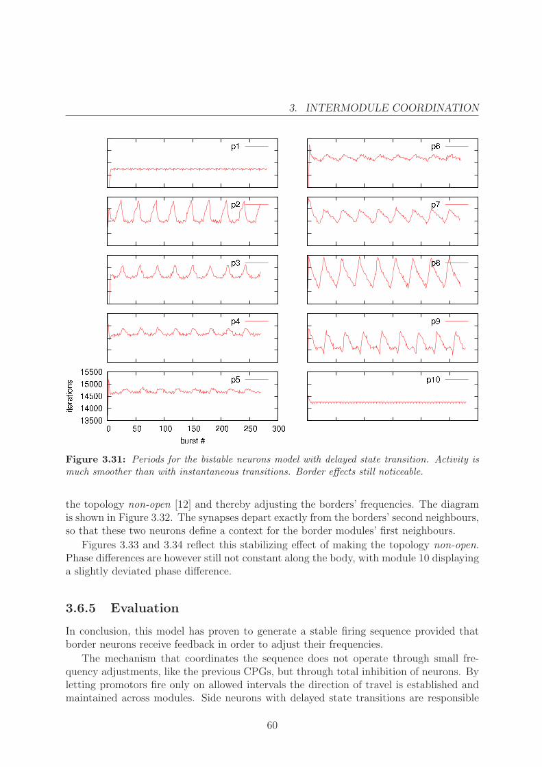
3. INTERMODULE COORDINATION
r
Figure 3.31: Periods for the bistable neurons model with delayed state transition. Activity ismuch smoother than with instantaneous transitions. Border effects still noticeable.
the topology non-open [12] and thereby adjusting the borders’ frequencies. The diagramis shown in Figure 3.32. The synapses depart exactly from the borders’ second neighbours,so that these two neurons define a context for the border modules’ first neighbours.
Figures 3.33 and 3.34 reflect this stabilizing effect of making the topology non-open.Phase differences are however still not constant along the body, with module 10 displayinga slightly deviated phase difference.
3.6.5 Evaluation
In conclusion, this model has proven to generate a stable firing sequence provided thatborder neurons receive feedback in order to adjust their frequencies.
The mechanism that coordinates the sequence does not operate through small fre-quency adjustments, like the previous CPGs, but through total inhibition of neurons. Byletting promotors fire only on allowed intervals the direction of travel is established andmaintained across modules. Side neurons with delayed state transitions are responsible
60

3.6. BISTABLE INTERMEDIATE NEURONS
,2
Figure 3.32: Bistable neurons with a non-open topology to cancel border effects caused by borderneurons not having any input. (remotors side symmetric, ommited for clarity)
Figure 3.33: Phase differences for the bistable neurons model with delayed state transition andborder effects compensation. P1 and P10 are now synchronized with the rest of the neurons.The synapse to P10 causes a slightly deviated behaviour.
61

3. INTERMODULE COORDINATION
r
Figure 3.34: Periods for the bistable neurons model with delayed state transition and bordereffects compensation. The two new synapses reduce border neurons’s frequency and the overallrhythm is stabilized.
for maintaining an efficient phase difference.
62

4
Discussion
Several approaches to the task of generating and coordinating a rhythmic movement fora modular robot have been proposed. Here we discuss what has been learnt from them.
4.1 CPG summary
Symmetric inhibition. The first proposed CPG was the ”symmetric inhibition”. Theidea is very simple: connect the neurons with inhibitory synapses to prevent in-phasebursting and see if they can burst in a stable sequence.
We have not studied whether this CPG always finds a stable firing sequence regardlessof initial conditions, but it can indeed find a stable sequence for some of them.
This circuit adjusts itself by performing small corrections in neurons’ frequency. Thisway phase difference can be adjusted by drift, that is, one neuron oscillating slower thanits neighbours and letting them “drift away”. As a result of this slow divergence, there isa long transient interval until a stable state is reached.
Drift may cause “sequence inversion”, when one neuron overtakes its neighbour, mean-ing that the direction of the firing sequence may be reversed. Since the proposed circuitlacks a mechanism to impose a particular direction of travel, the final direction once astable state has been found is unpredictable.
This, however, means that, if a suitable mechanism to define the direction of travel isdeveloped, like setting more specific initial conditions rather than random ones, the sameset of synapses could be used for both forward and backward travel. Another mechanismwould be needed for “on the fly” change of direction, nevertheless.
The “symmetric inhibition” CPG is a good candidate if the goal is to maintain analready established firing sequence, in both directions. However, other mechanisms shouldbe used to start the sequence.
Inhibitory loop. This CPG works by correcting one module’s frequency depending onits phase difference with its successor. Through a direct synapse from one module to
63

4. DISCUSSION
its neighbour, adjustments can be made to the successor module and through the loop,adjustments are also made to the predecessor module.
The CPG is designed to work in a particular direction. The circuit is capable itself bothof maintaining the direction of travel as well as of establishing it in the first place. Thetransient interval is relatively short, depending on synapse conductance. Real experienceis needed to determine if the transient is tolerable or indeed too long.
The “inhibitory loop” CPG is a very stable CPG, capable of starting and maintaininga stable sequence. The loop enables bidirectional adjustment to successor and predecessormodules.
Push-pull. The “push-pull” CPG is a very simple circuit, that nevertheless achieves avery stable phase difference between modules oscillating at similar frequencies.
This CPG works as a phase detector. The net effect of the two synapses, one excitatoryand one inhibitory, projected onto the successor module depend on the exact phase of thecycle on which the postsynaptic neuron finds itself. This way, modules can be speededup or slowed down until the desired phase difference is achieved.
The projected synapses go only one way. This means that information flow is unidi-rectional. Predecessor modules cannot process information coming from later modules.
One side effect of unidirectional information flow is that the first module oscillatesfaster than the rest. Since it does not receive any input, its frequency is unaffected, beingit its nominal frequency. All other modules oscillate always at a lower frequency, so astable phase difference (between the first modules) is impossible to achieve.
The “push-pull” CPG is able to achieve stable phase differences provided that adjacentmodules oscillate at approximately the same frequency. As it is presented here, the lack offeedback to earlier modules prevents the adjustment of the first module’s frequency to itssuccessor’s and causes periodic variations in frequency of the second and third modules.
Bistable neurons. The “bistable neuron” CPGs work not through frequency adjust-ment, but through complete inhibition of neurons. The endogenous rythmic nature ofneurons provides for an intermitent inhibitory activity. Topology then drives the systemin order to create a wave of succesive inhibitions and activations, defining allowed intervalsin which promotor and remotor neurons may fire. This mechanism defines a consistentdirection of travel and prevents sequence inversion.
The effect of strong inhibition is to “erase” the past, setting the system in a givenstate independent of initial conditions. As a result, this CPG might be very resilient toperturbations.
Lack of feedback to border neurons again prevents complete synchronization. However,we provide a model with two synapses that counteract this effect. As shown, just byestablishing these two synapses that correct the border modules’ frequencies, the CPG isable to achieve a constant phase difference among all of its modules.
64

4.1. CPG SUMMARY
4.1.1 Features
Not all CPGs display the same set of behaviours. This table tries to summarize whatthey can and cannot do:
Reversible Bidirectional
information
flow
Free of bor-
der effects
Fast conver-
gence
Symmetrical inhibition Y Y Y NInhibitory loop N Y Y YPush-pull N N N NBistable neurons (without bordersynapses)
N Y/N N Y
Bistable neurons (with bordersynapses)
N Y/N Y Y
Reversibility is here considered a feature, but it must be noted that the only reversibleCPG is also the only one that is not capable of defining a direction of travel.
The “bistable neurons” CPGs have bidirectional information flow indirectly. Promotor[remotor] neurons are not directly connected to each other, but one module can affect bothof its neighbours through their bistable ’B’ neurons.
4.1.2 Complexity
Another simple way to compare the CPGs is to sum the number of neurons and synapsesand divide it by the number of modules. We call this naive measure “complexity”:
C =Neurons + Synapses
Modules(4.1)
Considering all experiments have been carried out on a robot with 10 modules, theseare the results (only the promotor side is measured, since all CPGs are symmetric):
CPG Complexity
Symmetrical inhibition 2.8Inhibitory loop 5.5Push-pull 2.8Bistable neurons (without border synapses) 4.2Bistable neurons (with border synapses) 4.4
As expected, CPGs with higher complexity yield the most stable results, and CPGswith similar complexity have similar capabilities. For example, “push-pull” and “symmet-rical inhibition” have similar complexity values. It may seem that their results are verydifferent, but one should consider the tradeoffs of each CPG: while “push-pull” achievesvery stable phase differences, it lacks the ability to be reversible, as is the case for thelatter.
65

4. DISCUSSION
Likewise “inhibitory loop” provides stable phase differences, bidirectional informationflow, does not suffer from border effects and has the highest complexity. The bistableneurons have almost the same set of features except for the bidirectionality of informationflow, since promotor [remotor] neurons are not directly connected among them.
This yields a very interesting question: can features be quantified? Is there a minimumcomplexity that a CPG must have to display a certain set of features? Intuition says itmust be so. Moreover, it does not take the same amount of resources to counteractborder effects (only two synapses in “bistable neurons”) as to implement bidirectionalinformation flow, which would be proportional to the number of modules.
4.2 Symmetry
In general, it could be said that symmetry is to be avoided. This is not to say that nosymmetry should appear, rather that it must be broken at some level. If topology issymmetric, like the first symmetrical model proposed, then initial conditions must breakthe symmetry. This CPG has the basic ability of adjusting itself to a stable sequence buthas no mechanism to determine the direction of movement, so both directions are equallylikely given random initial conditions.
If activation of the modules is symmetric, that is, in-phase or anti-phase synchronized,there will not appear any propagating wave that makes the robot undulate, but ratherthere will be a standing wave. In conclusion, activations must be periodic but not sym-metric, i.e., there must be a constant phase difference accross modules. Otherwise thegenerated movement may not be efficient. Parity synchronization modes shown above arean example of symmetry to avoid.
4.3 Coupling strength
Weak coupling is a mechanism to exchange information among modules without severelyaltering the receiver’s behaviour. It allows each module to keep its activity seeminglyunaffected and independent while at the same time coordination is being “negociated”.The disadvantage is that for large systems convergence can be very slow if initial statesare sufficiently different.
On the other hand, strong inhibition can sharply change the receiver’s activity. Thismechanism allows for a faster convergence to a stable state, independent of initial con-ditions, and a faster response to changes. This is also a good mechanism to preventagainst perturbations, since strong coupling has a resetting effect that erases the past,thus isolating perturbations in a small time window.
Probably the best approach is to combine both mechanisms and have different con-nectivities acting at different times: one with stronger coupling to drive the system to aknown state (for starting and stopping the movement, or to recover from perturbations)and a weaker system to maintain activity once the stronger one has been shut off.
66

4.4. COUPLING SIGN
4.4 Coupling sign
While our first approach was to use inhibitory synapses only, this work has shown thatexcitatory coupling can also be useful.
Inhibitory synapses act to prevent in-phase synchronization and regulate oscillationfrequency. In general, when one module receives an inhibitory current, its frequency isdecreased. This is the cause for phase drift in the absence of feedback to the presynapticneuron.
In some cases, however, inhibition may cause an increase in frequency. If the timing isright, inhibition may shorten a neurons’ bursts but leave its recovery process unaffected,thereby shortening bursting period.
Excitatory synapses, on the other hand, promote in-phase synchronization. Takingadvantage of the delayed effect of chemical synapses, excitatory coupling can be used toachieve a constant delay between coupled modules.
The push-pull model has shown that these types of coupling are not exclusive, nor arethey equivalent to a weaker version of one of them when used simultaneously. Indeed,using both simultaneously we have constructed a stable phase detector.
4.5 Topology
It is very important that all modules share information, that is, send and receive stimuli.CPGs based on inhibition will suffer border effects if border neurons do not have anyfeedback. If this is the case, they will not have any means to adapt their frequency ofoscillation to that of the rest of the modules. As a consecuence, the system will not beable to achieve stable phase differences among them.
We have shown that it is possible to coordinate modules on a global scale by usingfirst neighbours only connections. This is however not very resistant to failure sincemalfunction in one module will comletely break the chain of communication. Projectionsto further modules and redundant communications will certainly provide richer dynamicsand better fault tolerance.
67

4. DISCUSSION
68

5
Future work
The first obvious step is to implement these models in a real robot. All models have beentested in a simulator, but several details have been left out.
One of them is that motors do not react instantaneously. The servomotors with whichthe actual robot is built receive a command specifying the desired position to which itshould rotate. Then, a PIC controller adjusts rotation speed depending on the distanceto the desired angle.
This poses two questions. The first one is if the models implemented on a computercan coordinate such a robot built on such motors. The current approach is to simulatethe models on a computer and send the corresponding commands to the motors, withoutreceiving any feedback on their position. This question amounts to whether we can adjustour simulation time so that motor movements can be considered instantaneous.
The second question is, given that the above fails, how we can integrate the informationabout motor position in the coordination of the movement. This links with one of ourwork lines which is integration of sensory feedback.
Once we have a model that effectively coordinates the real robot, the next step will beto integrate information about the environment and the robot itself in the generation ofmotor sequences. The goal is that the robot must be able to generate different behavioursdepending on external conditions (terrain, unforeseen perturbations) as well as on internalconditions (malfunction, non-instantaneous movements).
Along this line we will introduce multicoding neurons. These are neurons that canchange their interspike interval distribution, using it as a signature. Receivers that arecapable of decoding this distribution will be able to selectively react to messages and evendiscriminate among senders. This will provide the robot with a much richer sensitivity tochanging conditions due to a richer context awareness.
Finally, we will explore different topologies for the robot. This work has only consid-ered propagating waves in one plane. Actually, the robot can be configured so that somemodules oscillate in one plane and others in a perpendicular plane, allowing for a muchricher set of movements. Also, this work has only considered modules lined up in one di-mension. It would be interesting to explore bidimensional or tridimensional arrangements,symmetric and asymmetric, but this is a larger term goal.
69

5. FUTURE WORK
70
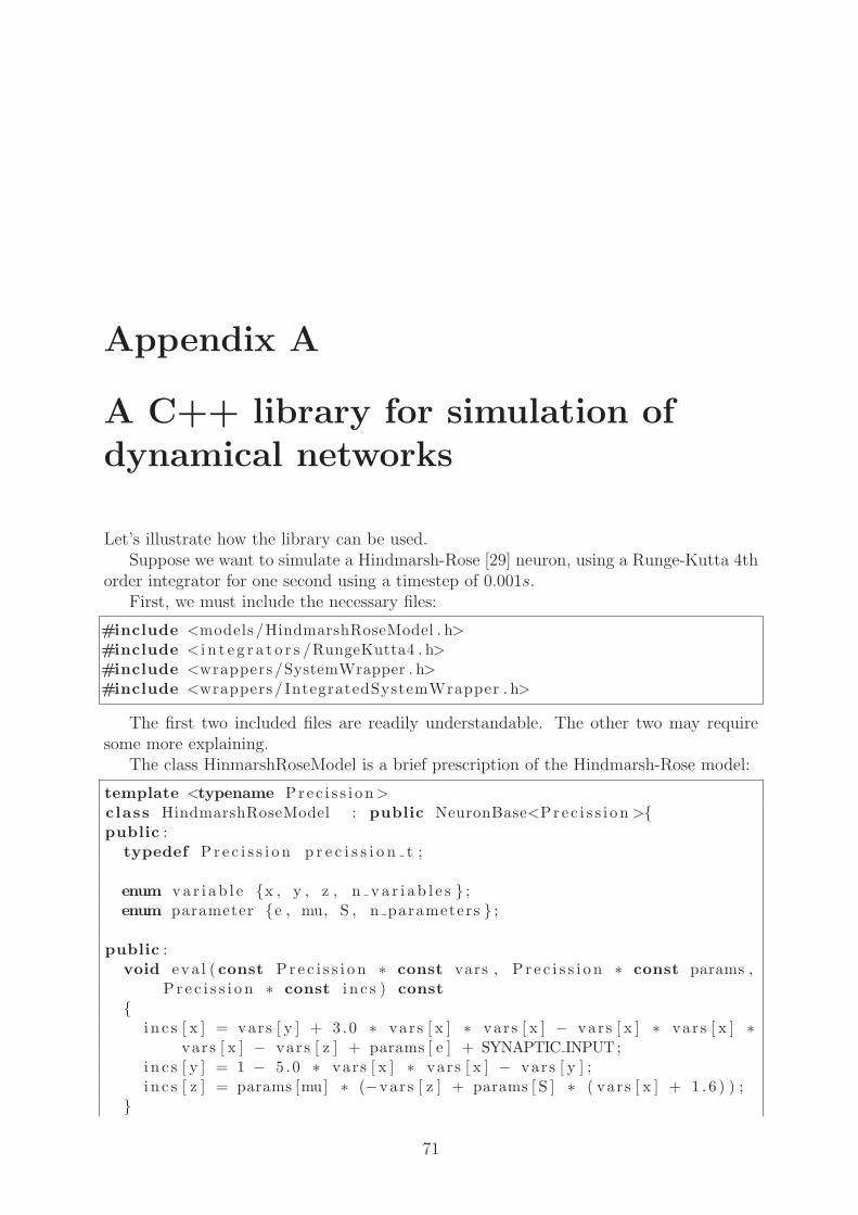
Appendix A
A C++ library for simulation of
dynamical networks
Let’s illustrate how the library can be used.Suppose we want to simulate a Hindmarsh-Rose [29] neuron, using a Runge-Kutta 4th
order integrator for one second using a timestep of 0.001s.First, we must include the necessary files:
#include <models/HindmarshRoseModel . h>#include < i n t e g r a t o r s /RungeKutta4 . h>#include <wrappers /SystemWrapper . h>#include <wrappers / IntegratedSystemWrapper . h>
The first two included files are readily understandable. The other two may requiresome more explaining.
The class HinmarshRoseModel is a brief prescription of the Hindmarsh-Rose model:
template <typename Prec i s s i on >class HindmarshRoseModel : public NeuronBase<Prec i s s i on >{public :
typedef Pr e c i s s i o n p r e c i s s i o n t ;
enum va r i ab l e {x , y , z , n v a r i a b l e s } ;enum parameter {e , mu, S , n parameters } ;
public :void eva l ( const Pr e c i s s i o n ∗ const vars , P r e c i s s i o n ∗ const params ,
P r e c i s s i o n ∗ const i n c s ) const
{i n c s [ x ] = vars [ y ] + 3 .0 ∗ vars [ x ] ∗ vars [ x ] − vars [ x ] ∗ vars [ x ] ∗
vars [ x ] − vars [ z ] + params [ e ] + SYNAPTIC INPUT;i n c s [ y ] = 1 − 5 .0 ∗ vars [ x ] ∗ vars [ x ] − vars [ y ] ;i n c s [ z ] = params [mu] ∗ (−vars [ z ] + params [ S ] ∗ ( vars [ x ] + 1 . 6 ) ) ;
}
71

APPENDIX A. A C++ LIBRARY FOR SIMULATION OF DYNAMICAL
NETWORKS
} ;
It contains no data members: this class cannot store any value neither for the variablesnor for the parameters. Model classes must be simple by design, so that adding a newmodel has as little implementation details as possible.
It is through wrapping this class that new functionality can be added. For instance,the class SystemWrapper adds storage functionality and methods to set and get the valuesof the variables and parameters of the model:
typedef HindmarshRoseModel<double> Model ;typedef SystemWrapper<Model> System ;typedef IntegratedSystemWrapper<System , RungeKutta4> Neuron ;
Here you see why they are called wrappers. In this case we use two wrappers: Sys-temWrapper to add storage access funcionality and IntegratedSystemWrapper to addstepping funcionality.
Here is the main body of our program:
int main ( ){
Neuron : : ConstructorArgs args ;
a rgs [ Neuron : : e ] = 3 . 0 ;args [ Neuron : :mu] = 0 . 0021 ;args [ Neuron : : S ] = 4 ;
Neuron n( args ) ;
const double s tep = 0 . 0 0 1 ;
for ( int i = 0 ; i < 1000 ; i++){n . s tep ( s tep ) ;
cout << n . get (Neuron : : x ) << endl ;}
return 0 ;}
A.1 Using synapses
To add synapses (diffusion synapses, in this example) to our simulation we must add theselines to the head of our program:
#include <include/ D i f f u s i onSynaps i s . h>
72

A.2. SIMULATING ITERATED MAPS
typedef Di f fu s i onSynaps i s <Neuron , Neuron , RungeKutta4> Syn ;
The three template parameters are: type of the presynaptic neuron, type of the post-synaptic neuron and integrator type.
We can now instantiate it and step it:
. . .Neuron n( args ) ;Neuron n2 ( args ) ;
Syn : : ConstructorArgs synargs ={0.5 , 10 , 0 , 9 , 1 . 5 , 1 , 0 . 0 1} ;
Syn syn (n , Neuron : : x , n2 , Neuron : : x , synargs ) ;
const double s tep = 0 . 0 0 1 ;
for ( int i = 0 ; i < 1000 ; i++){syn . s tep ( s tep ) ;
n . s tep ( s tep ) ;n2 . s tep ( s tep ) ;
cout << n . get (Neuron : : x ) << ’ ’ << n2 . get (Neuron : : x ) << endl ;}
return 0 ;}
Here we see another way of filling out the constructor arguments. This way may beconfusing, because the name of the parameter is not explicitly specified, but it comes inhandy for long lists of arguments like this one.
When constructing the synapse object we need to specify the pre- and postsynapticneurons as well as the variables to be measured. Once the object is constructed, it has astep method like any other dynamical system of the library.
Note that synapses should be stepped before any other element in the network, sothat postsynaptic neurons know their right input when stepping.
A.2 Simulating iterated maps
Discrete maps are not different from differential equations from this library’s perspective.As before, we need to include the model, the wrappers we need and the integrator to use:
#include <models/RulkovMapModel . h>#include < i n t e g r a t o r s / Stepper . h>
73

APPENDIX A. A C++ LIBRARY FOR SIMULATION OF DYNAMICAL
NETWORKS
#include <wrappers /SystemWrapper . h>#include <wrappers / IntegratedSystemWrapper . h>
Note that we are using the Stepper integrator now. The rest of the simulation is exactlythe same, except for one point: the step method still accepts a timestep parameter, butit is not taken into account, the model always steps one time unit.
A.3 Adding new models
Adding a new neuron model is really easy using the following template:
#ifndef MODEL H#define MODEL H
#include <cmath>#include ‘ ‘ . . / include/NeuronBase . h ’ ’
template <typename Prec i s s i on >class Model : public NeuronBase<Prec i s s i on >{public :
typedef Pr e c i s s i o n p r e c i s s i o n t ;
public :void eva l ( const Pr e c i s s i o n ∗ const vars , P r e c i s s i o n ∗ const params ,
P r e c i s s i o n ∗ const i n c s ) const
{}
} ;
#endif /∗MODEL H ∗/
One only needs to add:
• A variables enum, including the names of all involved variables, terminated with“n variables”.
• A parameters enum, including the names of all involved parameters, terminatedwith “n parameters”.
• Equations to the eval method. For an equation of the form x = αx + βy one shouldwrite
i n c s [ x ] = params [ alpha ] ∗ vars [ x ] + params [ beta ] ∗ vars [ y ] ;
If the model is an iterated map, it is almost the same, except for the eval method:
74

A.4. AVAILABLE WRAPPERS
• For a map of the form xn = αxn−1 + βyn−1 write:
i n c s [ x ] = params [ alpha ] ∗ vars [ x ] + params [ beta ] ∗ vars [ y ] ;
Now we calculate the next point directly, not the increment. The idea is that thestatement always ressembles the mathematical expression.
A.4 Available wrappers
These are all the wrappers available at the moment in the library.
A.4.1 SystemWrapper
When applied to a model class “Model”, this wrapper adds a member array called“m variables” of size “Model::n variables” and another one called “m parameters” of sizeModel::n parameters”.
Besides, the following methods are defined:
p r e c i s s i o n t get ( v a r i ab l e var ) const
{return m var iab l e s [ var ] ;
}
void s e t ( v a r i ab l e var , p r e c i s s i o n \ t va lue ){
m var iab l e s [ var ] = value ;}
p r e c i s s i o n t get ( parameter param) const
{return m parameters [ param ] ;
}
void s e t ( parameter param , p r e c i s s i o n t va lue ){
m parameters [ param ] = value ;}
A.4.2 IntegratedSystemWrapper
This wrapper takes a system class and an integrator class as template arguments andprovides a method to step the model:
75

APPENDIX A. A C++ LIBRARY FOR SIMULATION OF DYNAMICAL
NETWORKS
void s tep ( p r e c i s s i o n t h){
/∗ Allow system s p e c i f i c s t ep ac t i on s∗/
pr e s t ep (h) ;
I n t e g r a t o r : : s t ep (∗ this , h , System : : m var iab les ,System : : m parameters ) ;
po s t s t ep (h) ;}
A.4.3 TimeWrapper
This class adapts models working at different time scales. At construction time it receivesan argument specifying how many calls to the “step” method will cause an actual step ofthe model:
TimeWrapper ( ConstructorArgs const &args , int s ub s t e p s p e r c y c l e = 1): m subs t ep s pe r cyc l e ( s ub s t e p s p e r c y c l e ) , m count (0 ) ,IntegratedSystem ( args )
{}
Due to this restriction, this wrapper should be applied the last, because other wrappersdo not know yet how to receive this argument in their constructor (a future implementationwill include the solution described in [27]).
It also provides the following step method:
void s tep ( p r e c i s s i o n h){
m count++;
i f ( m count > m subs t ep s pe r cyc l e ) {m count = 0 ;
IntegratedSystem : : s tep (h) ;}
}
76

A.4. AVAILABLE WRAPPERS
A.4.4 SerializableWrapper
SerializableWrapper adds serializable capabilities: one method to store variables in astream (it could be easily extended to also store parameters), and one to load them froma stream:
void save ( std : : ostream &os ) const
{for ( int i = 0 ; i < System : : n v a r i a b l e s ; i++){
os << System : : m var iab l e s [ i ] << ” ” ;}
}
void load ( std : : i s t ream &i s ){
for ( int i = 0 ; i < System : : n v a r i a b l e s ; i++){i s >> System : : m var iab l e s [ i ] ;
}}
77

APPENDIX A. A C++ LIBRARY FOR SIMULATION OF DYNAMICAL
NETWORKS
78

Bibliography
[1] G. Orlovsky, T. G. Deliagina, and S. Grillner, Neuronal Control of Locomotion. Ox-ford university press, November 1999.
[2] C. Tin and C.-S. Poon, “Internal models in sensorimotor integration: perspectivesfrom adaptive control theory,” Journal of Neural Engineering, vol. 2, pp. S147+,September 2005.
[3] N. G. Hatsopoulos, “Coupling the neural and physical dynamics in rhythmic move-ments.,” Neural Comput, vol. 8, pp. 567–581, April 1996.
[4] A. I. Selverston, M. I. Rabinovich, H. D. Abarbanel, R. Elson, A. Szucs, R. D. Pinto,R. Huerta, and P. Varona, “Reliable circuits from irregular neurons: A dynamicalapproach to understanding central pattern generators,” Journal of Physiology-Paris,vol. 94, pp. 357–374, December 2000.
[5] R. C. Elson, A. I. Selverston, H. D. Abarbanel, and M. I. Rabinovich, “Inhibitorysynchronization of bursting in biological neurons: Dependence on synaptic time con-stant,” J Neurophysiol, vol. 88, pp. 1166–1176, September 2002.
[6] C. Van Vreeswijk, L. F. Abbott, and B. G. Ermentrout, “When inhibition not ex-citation synchronizes neural firing,” Journal of Computational Neuroscience, vol. 1,pp. 313–321, December 1994.
[7] P. Varona, M. I. Rabinovich, A. I. Selverston, and Y. I. Arshavsky, “Winnerlesscompetition between sensory neurons generates chaos: A possible mechanism formolluscan hunting behavior,” Chaos: An Interdisciplinary Journal of Nonlinear Sci-ence, vol. 12, no. 3, pp. 672–677, 2002.
[8] F. B. Rodrıguez, P. Varona, R. Huerta, M. I. Rabinovich, and H. D. I. Abarbanel,“Richer network dynamics of intrinsically non-regular neurons measured throughmutual information,” in Connectionist Models of Neurons, Learning Processes andArtificial Intelligence : 6th International Work-Conference on Artificial and NaturalNeural Networks, IWANN 2001 Granada, Spain, June 13-15, 2001, Proceedings, PartI, vol. 2084/2001, pp. 490+, Springer Berlin / Heidelberg, 2001.
79

BIBLIOGRAPHY
[9] F. K. Skinner, N. Kopell, and E. Marder, “Mechanisms for oscillation and frequencycontrol in reciprocally inhibitory model neural networks,” Journal of ComputationalNeuroscience, vol. 1, June 1994.
[10] X.-J. Wang and J. Rinzel, “Alternating and synchronous rhythms in reciprocallyinhibitory model neurons,” Neural Comput., vol. 4, pp. 84–97, January 1992.
[11] G. A. Bekey, Autonomous Robots, From Biological Inspiration to Implementation andControl, vol. 24. New York, NY, USA: MIT Press, March 2005.
[12] R. Huerta, P. Varona, M. I. Rabinovich, and H. D. Abarbanel, “Topology selectionby chaotic neurons of a pyloric central pattern generator.,” Biol Cybern, vol. 84,January 2001.
[13] J. Gonzalez-Gomez, E. Aguayo, and E. Boemo, “Locomotion of a modular worm-likerobot using a fpga-based embedded microblaze soft-processor,” in 7th InternationalConference on Climbing and Walking Robots, September 2004.
[14] A. Kamimura, H. Kurokawa, E. Toshida, K. Tomita, S. Murata, and S. Kokaji, “Au-tomatic locomotion pattern generation for modular robots,” in IEEE InternationalConference on Robotics and Automation, vol. 1, pp. 714–720 vol.1, 2003.
[15] A. Ijspeert and J. Kodjabachian, “Evolution and development of a central patterngenerator for the swimming of a lamprey,” 1998.
[16] J. Ayers, C. Wilbur, and C. Olcott, “Lamprey robots,” in International Symposiumon Aqua Biomechanisms (T. Wu and N. Kato, eds.), Tokai University, 2000.
[17] P. Manoonpong, T. Geng, T. Kulvicius, B. Porr, and F. Worgotter, “Adaptive, fastwalking in a biped robot under neuronal control and learning,” PLoS ComputationalBiology, May 2007.
[18] C. Koch, Biophysics of Computation: Information Processing in Single Neurons(Computational Neuroscience). Oxford University Press, November 1998.
[19] C. Aguirre, D. Campos, P. Pascual, and E. Serrano, “A model of spiking-burstingneuronal behavior using a piecewise linear two-dimensional map,” pp. 130–135, 2005.
[20] E. M. Izhikevich and F. Hoppensteadt, “Classification of bursting mappings,” Inter-national Journal of Bifurcation and Chaos, vol. 14, no. 11, pp. 3847–3854, 2004.
[21] N. F. Rulkov, “Modeling of spiking-bursting neural behavior using two-dimensionalmap,” Physical Review E, vol. 65, pp. 041922+, April 2002.
[22] A. Destexhe, Z. F. Mainen, and T. J. Sejnowski, “An efficient method for comput-ing synaptic conductances based on a kinetic model of receptor binding,” NeuralComput., vol. 6, pp. 14–18, January 1994.
80
BIBLIOGRAPHY
[23] E. Gamma, R. Helm, R. Johnson, and J. Vlissides, Design Patterns. Addison-WesleyProfessional, January 1995.
[24] J. Siek and A. Lumsdaine, “Concept checking: Binding parametric polymorphismin c++,” in Proceedings First Workshop on C++ Template Programming, (Erfurt,Germany), 2000.
[25] J. O. Coplien, “Curiously recurring template patterns,” C++ Rep., vol. 7, pp. 24–27,February 1995.
[26] Y. Smaragdakis and D. Batory, “Mixin-based programming in c++,” 2000.
[27] U. W. Eisenecker, F. Blinn, and K. Czarnecki, “A solution to the constructor-problemof mixin-based programming in c++,” in First Workshop on C++ Template Pro-gramming, Erfurt, Germany, October 2000.
[28] W. B. Kristan, “Neuroscience: A push-me pull-you neural design,” Science, vol. 315,pp. 339–340, January 2007.
[29] J. L. Hindmarsh and R. M. Rose, “A model of neuronal bursting using three coupledfirst order differential equations,” Proceedings Of The Royal Society Of London. Se-ries B, Containing Papers Of a Biological Character. Royal Society (Great Britain),vol. 221, pp. 87–102, March 1984.
81