TR 125 963 - V14.0.0 - Universal Mobile … First system-level study (Ericsson) ... significant...

ETSI TR 125 963 V14.0.0 (2017-04)

Universal Mobile Telecommunications System (UMTS); Feasibility study on interference cancellation for

UTRA FDD User Equipment (UE) (3GPP TR 25.963 version 14.0.0 Release 14)

TECHNICAL REPORT

ETSI

ETSI TR 125 963 V14.0.0 (2017-04)13GPP TR 25.963 version 14.0.0 Release 14

Reference RTR/TSGR-0425963ve00

Keywords UMTS

ETSI

650 Route des Lucioles F-06921 Sophia Antipolis Cedex - FRANCE

Tel.: +33 4 92 94 42 00 Fax: +33 4 93 65 47 16

Siret N° 348 623 562 00017 - NAF 742 C

Association à but non lucratif enregistrée à la Sous-Préfecture de Grasse (06) N° 7803/88

Important notice

The present document can be downloaded from: http://www.etsi.org/standards-search

The present document may be made available in electronic versions and/or in print. The content of any electronic and/or print versions of the present document shall not be modified without the prior written authorization of ETSI. In case of any

existing or perceived difference in contents between such versions and/or in print, the only prevailing document is the print of the Portable Document Format (PDF) version kept on a specific network drive within ETSI Secretariat.

Users of the present document should be aware that the document may be subject to revision or change of status. Information on the current status of this and other ETSI documents is available at

https://portal.etsi.org/TB/ETSIDeliverableStatus.aspx

If you find errors in the present document, please send your comment to one of the following services: https://portal.etsi.org/People/CommiteeSupportStaff.aspx

Copyright Notification

No part may be reproduced or utilized in any form or by any means, electronic or mechanical, including photocopying and microfilm except as authorized by written permission of ETSI.

The content of the PDF version shall not be modified without the written authorization of ETSI. The copyright and the foregoing restriction extend to reproduction in all media.

© European Telecommunications Standards Institute 2017.

All rights reserved.

DECTTM, PLUGTESTSTM, UMTSTM and the ETSI logo are Trade Marks of ETSI registered for the benefit of its Members. 3GPPTM and LTE™ are Trade Marks of ETSI registered for the benefit of its Members and

of the 3GPP Organizational Partners. oneM2M logo is protected for the benefit of its Members

GSM® and the GSM logo are Trade Marks registered and owned by the GSM Association.

http://www.etsi.org/standards-search

https://portal.etsi.org/TB/ETSIDeliverableStatus.aspx

https://portal.etsi.org/People/CommiteeSupportStaff.aspx

ETSI


Intellectual Property Rights IPRs essential or potentially essential to the present document may have been declared to ETSI. The information pertaining to these essential IPRs, if any, is publicly available for ETSI members and non-members, and can be found in ETSI SR 000 314: "Intellectual Property Rights (IPRs); Essential, or potentially Essential, IPRs notified to ETSI in respect of ETSI standards", which is available from the ETSI Secretariat. Latest updates are available on the ETSI Web server (https://ipr.etsi.org/).

Pursuant to the ETSI IPR Policy, no investigation, including IPR searches, has been carried out by ETSI. No guarantee can be given as to the existence of other IPRs not referenced in ETSI SR 000 314 (or the updates on the ETSI Web server) which are, or may be, or may become, essential to the present document.

Foreword This Technical Report (TR) has been produced by ETSI 3rd Generation Partnership Project (3GPP).

The present document may refer to technical specifications or reports using their 3GPP identities, UMTS identities or GSM identities. These should be interpreted as being references to the corresponding ETSI deliverables.

The cross reference between GSM, UMTS, 3GPP and ETSI identities can be found under http://webapp.etsi.org/key/queryform.asp.

Modal verbs terminology In the present document "should", "should not", "may", "need not", "will", "will not", "can" and "cannot" are to be interpreted as described in clause 3.2 of the ETSI Drafting Rules (Verbal forms for the expression of provisions).

"must" and "must not" are NOT allowed in ETSI deliverables except when used in direct citation.

https://ipr.etsi.org/

http://webapp.etsi.org/key/queryform.asp

https://portal.etsi.org/Services/editHelp!/Howtostart/ETSIDraftingRules.aspx

ETSI


Contents

Intellectual Property Rights ................................................................................................................................ 2

Foreword ............................................................................................................................................................. 2

Modal verbs terminology .................................................................................................................................... 2

Foreword ............................................................................................................................................................. 5

Introduction ........................................................................................................................................................ 5

1 Scope ........................................................................................................................................................ 7

2 References ................................................................................................................................................ 7

3 Abbreviations ......................................................................................................................................... 10

4 Receiver methods ................................................................................................................................... 10

4.1 Two-branch interference mitigation ................................................................................................................. 10

4.2 One-branch interference mitigation .................................................................................................................. 12

5 Network scenarios .................................................................................................................................. 12

6 Interference modelling ........................................................................................................................... 13

6.1 General ............................................................................................................................................................. 13

6.2 Statistical measures .......................................................................................................................................... 14

6.2 Interference profile based on median values .................................................................................................... 14

6.3 Interference profiles based on weighted average throughput gain ................................................................... 22

6.3.0 General ........................................................................................................................................................ 22

6.3.1 0 dB geometry ............................................................................................................................................. 23

6.3.2 -3 dB geometry ........................................................................................................................................... 23

6.4 Interference profiles based on field data ........................................................................................................... 24

6.5 Summary .......................................................................................................................................................... 25

7 Transmitted code/power characteristics ................................................................................................. 26

7.0 General ............................................................................................................................................................. 26

7.1 Transmitted code and power characteristic in case of HSDPA ........................................................................ 26

7.1.1 Common channels for serving and interfering cells ................................................................................... 26

7.1.2 Serving cell ................................................................................................................................................. 27

7.1.2.1 Transmitted code and power characteristics for HSDPA+R’99 scenario ............................................. 27

7.1.2.2 Transmitted code and power characteristics for HSDPA-only scenario ............................................... 28

7.1.3 Interfering cells ........................................................................................................................................... 29

7.1.3.1 Transmitted code and power characteristics for HSDPA+R’99 scenario ............................................. 29

7.1.3.2 Transmitted code and power characteristics for HSDPA-only scenario ............................................... 30

7.1.4 Model for the power control sequence generation ...................................................................................... 31

8 Link performance characterization ......................................................................................................... 31

8.0 General ............................................................................................................................................................. 31

8.1 Overview .......................................................................................................................................................... 31

8.2 Simulation results ............................................................................................................................................. 32

8.2.1 Types 2 and 2i - median DIP values ........................................................................................................... 32

8.2.2 Types 3 and 3i - median DIP values ........................................................................................................... 33

8.2.3 Weighted DIPS: geometries -3 & 0 dB ....................................................................................................... 34

8.2.4 Revised DIP: geometry -3 dB ..................................................................................................................... 35

8.2.5 Power control .............................................................................................................................................. 35

8.2.6 Field based DIP ........................................................................................................................................... 35

8.2.7 Types 2i / 2 receivers: weighted & revised DIPS ....................................................................................... 36

8.3 Appendix .......................................................................................................................................................... 36

9 System performance characterization..................................................................................................... 58

9.0 General ............................................................................................................................................................. 58

9.1 First system-level study (Ericsson) .................................................................................................................. 58

9.1.1 Simulation setup ......................................................................................................................................... 58

9.1.2 Simulation results ....................................................................................................................................... 59

ETSI


9.2 Second system-level study (Nokia) .................................................................................................................. 61

9.2.1 Simulation setup for second study .............................................................................................................. 61

9.2.2 Simulation results for second study ............................................................................................................ 63

9.3 Conclusions ...................................................................................................................................................... 66

10 Receiver implementation issues ............................................................................................................. 66

11 Conclusions ............................................................................................................................................ 67

Annex A: Change history ...................................................................................................................... 69

History .............................................................................................................................................................. 70

ETSI


Foreword This Technical Report has been produced by the 3rd Generation Partnership Project (3GPP).

The contents of the present document are subject to continuing work within the TSG and may change following formal TSG approval. Should the TSG modify the contents of the present document, it will be re-released by the TSG with an identifying change of release date and an increase in version number as follows:

Version x.y.z

where:

x the first digit:

1 presented to TSG for information;

2 presented to TSG for approval;

3 or greater indicates TSG approved document under change control.

y the second digit is incremented for all changes of substance, i.e. technical enhancements, corrections, updates, etc.

z the third digit is incremented when editorial only changes have been incorporated in the document.

Introduction A study item for further improved minimum performance requirements for UMTS/HSDPA UE (FDD) was approved at the 3GPP RAN #30 meeting [1]. This technical report summarizes the work that RAN4 has accomplished in this study item to assess the feasibility of both one-branch and two-branch interference cancellation/mitigation UE receivers. These receivers attempt to cancel the interference that arises from users operating outside the serving cell. This type of interference is also referred to as 'other-cell' interference. In past link level evaluations, this type of interference has been modelled as AWGN, and as such can not be cancelled. The study item has developed models for this interference in terms of the number of interfering Node Bs to consider, and their powers relative to the total other cell interference power, the latter ratios referred to as Dominant Interferer Proportion (DIP) ratios. DIP ratios have been defined based on three criteria; median values of the corresponding cumulative density functions, weighted average throughput gain, and field data. In addition, two network scenarios are defined, one based solely on HSDPA traffic (HSDPA-only), and the other based on a mixture of HSDPA and Rel. 99 voice traffic (HSDPA+R99).

Interference aware receivers, referred to as type 2i and type 3i, were defined as extensions of the existing type 2 and type 3 receivers, respectively. The basic receiver structure is that of an LMMSE sub-chip level equalizer which takes into account not only the channel response matrix of the serving cell, but also the channel response matrices of the most significant interfering cells. HSDPA throughput estimates are developed using link level simulations, which include the other-cell interference model plus OCNS models for the serving and interfering cells based on the two network scenarios considered. In addition, system level performance is assessed to determine the gains that interference cancellation/mitigation receiver might provide in throughput and coverage. Complexity issues associated with implementing these types of receivers are also discussed. The content of each specific clause of the report is briefly described as follows.

Clause 1 of this document defines the scope and objectives of this feasibility study. Clause 4 describes the receiver methods that can be applied to one-branch and two-branch Interference Cancellation (IC) receivers. The reference receivers for the type 2i and type 3i are defined, both of which are based on LMMSE sub-chip level equalizers with interference-aware capabilities. Clause 5 describes the two network scenarios that were defined and used to generate the interference statistics, which were then used to develop the interference models described in clause 6. Clause 6 defines the interference models/profiles that were developed in order to assess the link level performance of IC receivers. The DIP ratio is defined as a key statistical measure, which forms the basis of the three types of interference profiles considered.

ETSI


Clause 7 defines the code and power characteristics of the signals transmitted by the serving and interfering cells for the two network scenarios defined in clause 5. These latter definitions essentially define the signal characteristics of the desired user, the common channels and the OCNS for both serving and interfering cells. Clause 8 summarizes the link level simulation results based on the assumptions developed in clauses 6 and 7, while clause 9 summarizes the system level performance characterization. Clause 10 discusses the possible receiver implementation losses for a two-branch, sub-chip based LMMSE equalizer with interference aware capabilities. Finally, clause 11 provides the relevant conclusions that can be taken from this study.

ETSI


1 Scope The objective of this study is to evaluate the feasibility and potential performance improvements of interference cancellation/mitigation techniques for UTRA FDD UE receivers, based on realistic network scenarios. Scope of the work includes:

- Determine realistic network scenarios.

- Determine suitable interference models for 'other cell' interference.

- Evaluate the feasibility of two-branch interference cancellation receivers through link and system level analysis and simulations.

- Evaluate feasibility of one-branch interference cancellation receivers through link and system level analysis and simulations.

2 References The following documents contain provisions which, through reference in this text, constitute provisions of the present document.

• References are either specific (identified by date of publication, edition number, version number, etc.) or non-specific.

• For a specific reference, subsequent revisions do not apply.

• For a non-specific reference, the latest version applies. In the case of a reference to a 3GPP document (including a GSM document), a non-specific reference implicitly refers to the latest version of that document in the same Release as the present document.

[1] RP-050764, "New Study Item Proposal: Further Improved Performance Requirements for UMTS/HSDPA UE", Cingular Wireless, RAN #30.

[2] R4-060514, "Reference structure for interference mitigation simulations with HSDPA and receiver diversity", Nokia, RAN4 #39.

[3] R4-060364, "Minutes of Ad Hoc on Further Improved Performance Requirements for UMTS/HSDPA UE (FDD)", Nokia, RAN4 #38.

[4] R4-060117, "Analysis for simulation scenario definition to interference mitigation studies", Nokia, RAN4#38.

[5] R4-060180, "Network Scenarios and Associated Interference Profiles for Evaluation of Generalized Interference Cancellation (IC) Receivers", Cingular, RAN4 #38.

[6] TR 25.848 v4.0.0, "Physical layer aspects of UTRA High Speed Downlink Packet Access (Release 4)".

[7] TR 25.896 V6.0.0 (2004-3), "Feasibility Study for Enhanced Uplink for UTRA FDD (Release 6)".

[8] R4-060959, "Throughput simulation results for Type 3 and Type 3i receivers with shadow fading and realistic DIP values for Ior/Ioc=0 dB", InterDigital, RAN4 #40.

[9] R4-061068, "Some observations on DIP values as a function of network geometries", TensorComm, RAN4 #40.

[10] R4-060512, "Analysis simulation results for scenario definition to interference mitigation studies", Nokia, RAN4 #39.

[11] R4-060391, "HSDPA Network Scenario and Associated Interference Profile for Evaluation of Generalized Interference Cancellation (IC) Receivers", Cingular/AT&T, RAN4 #39.

[12] R4-060369, "Observations on Other-Cell Interference Modelling", Motorola, RAN4 #39.

ETSI


[13] R4-060492, "Interferer Statistics for the UE IC Study Item," Qualcomm, RAN4 #39.

[14] TR 45.903, "Feasibility Study on Single Antenna Interference Cancellation (SAIC) for GSM Networks (Release 6)".

[15] R4-060648, "Minutes of Wednesday Evening Ad Hoc on Interference Mitigation", Cingular/AT&T, RAN4 #39.

[16] 3GPP RAN4 reflector e-mail, "Correction in DIPi and AWGN/Ioc values shown in R4-060648", May 31, 2006.

[17] R4-061080, "Minutes of Interference Cancellation Ad Hoc", Cingular/AT&T, RAN4 #40.

[18] R4-061183, "Throughput simulation results for type 3 and type 3i receivers based on an alternative method for determining DIP values", AT&T Labs, Inc. & Cingular Wireless, RAN4 #41.

[19] R4-070042, Throughput simulation results for type 3 and type 3i receivers for Ior/Ioc = -3 dB based on an alternative method for determining DIP values, AT&T Labs, Inc. & Cingular Wireless, RAN4 #42.

[20] R4-061241, "HSDPA Simulation Results for Type 3i with Weighted DIP Values", Motorola, RAN4 #41.

[21] R4-070041, Minutes of interim conference call on interference cancellation study item, AT&T Labs, Inc. & Cingular Wireless, RAN4 #42.

[22] R4-061315, "Interference data collection on a live UMTS network", Orange, RAN4 #41.

[23] R4-061309, "Interference Statistics Based on Field Measurements from an Operational UMTS/HSDPA Market", Cingular, AT&T and TensorComm, RAN4 #41.

[24] R4-061316, "Scenario definition for interference cancellation evaluation based on measurements taken in 3 UK's operational network", 3, RAN4 #41.

[25] R4-060593, "Further Thoughts on Scenario Definition for Studying Link Performance of Generalized IC Receivers", Ericsson, RAN4 #39.

[26] R4-060638, "Code Structure of Serving and Interfering Base Stations", Motorola, RAN4 #39.

[27] R4-060494, "Details of the Code Structure and Power Allocation for the HSDPA UE IC Case", Qualcomm, RAN4 #39.

[28] R4-060513, "Modelling of transmission for interference mitigation studies", Nokia, RAN4 #39.

[29] R4-060649, "Modelling of the code structure in serving and interfering base station for HSDPA", Nokia, RAN4, 39.

[30] R4-060885, "Discussion of realistic scenarios for Interference Cancellation", Ericsson, RAN4 #40.

[31] R4-070129, "Modelling of power control behaviour for OCNS", Nokia, RAN4 #42.

[32] R4-060841, Simulation Results for Type 2 and 2i Receivers for HSDPA+R99 Scenario, Motorola, RAN4 #40.

[33] R4-060842, Simulation Results for Type 3 and 3i Receivers for HSDPA+R99 Scenario, Motorola, RAN4 #40.

[34] R4-060884, Simulation results for Interference Cancellation (IC0 study item, Ericsson, RAN4 #40.

[35] R4-060953, HSDPA type 3i receiver simulation results, Fujitsu, RAN4 #40.

[36] R4-060954, HSDPA type 2i receiver simulation results, Fujitsu, RAN4 #40.

[37] R4-060957, Simulation results for agreed median DIP values, InterDigital Communications Corporation, RAN4 #40.

ETSI


[38] R4-060981, Simulation Results for HSDPA Type 2i and Type 3i Receivers, Intel Corp., RAN4 #40.

[39] R4-060983, Simulation Results for Type 2 and 2i Receivers for HSDPA Scenario, Motorola, RAN4 #40.

[40] R4-060984, Simulation Results for Type 3 and 3i Receivers for HSDPA Scenario, Motorola, RAN4 #40.

[41] R4-060909, Initial simulation results for HSDPA+R99 scenario, Nokia, RAN4 #40.

[42] R4-060939, Initial Simulation Results for Type 3i Receiver in HSDPA+R99 scenario, Panasonic, RAN4 #40.

[43] R4-061080, Minutes of Interference Cancellation Ad Hoc, Cingular Wireless / AT&T, RAN4 #40.

[44] R4-061176, Simulation results for HSDPA-Only scenario using Type 3 and Type 3i receivers, Ericsson, RAN4 #41.

[45] R4-061185, Ideal simulation results for HSDPA+R99 scenario, Nokia, RAN4 #41.

[46] R4-061186, Ideal simulation results for HSDPA-only scenario, Nokia, RAN4 #41.

[47] R4-061198, Simulation Results for Type 3i Receiver in HSDPA scenario, Panasonic, RAN4 #41.

[48] R4-061234, Simulation Results for Type 3 and 3i Receivers for the HSDPA scenario, Ior/Ioc=-3and 0 dB, InterDigital, RAN4 #41.

[49] R4-061246, Simulation results for Type 3 and Type 3i Receivers for HSDPA + R99 Scenario, Agere Systems, RAN4 #41.

[50] R4-061247, Simulation results for Type 3 and Type 3i Receivers for HSDPA Scenario, Agere Systems, RAN4 #41.

[51] R4-061260, HSDPA type3i receiver simulation results, Fujitsu, RAN4 #41.

[52] R4-0601279, Simulation Results for HSDPA Type 3i Receivers, Intel Corp., RAN4 #41.

[53] R4-061356, HSDPA Simulation Results for Type 3i with Weighted DIP Values, Motorola, RAN4 #41.

[54] R4-070044, Additional Link Level Simulation Results for Type 3 and Type 3i Receivers, AT&T/Cingular, RAN4 #42.

[55] R4-070045, Evaluation of Power Control Algorithms, AT&T/Cingular, RAN4 #42.

[56] R4-070061, HSDPA Simulation Results for Type 3i / 3 Receivers, Motorola, RAN4 #42.

[57] R4-070073, Simulation results for HSDP-only scenario using Type 3 and Type 3i receivers, LG Electronics, RAN4 #42.

[58] R4-070074, Simulation results for HSDPA+R'99 scenario using Type 3 and Type 3i receivers, LG Electronics, RAN4 #42.

[59] R4-070089, Simulation results for Type 3i receiver for Ior/Ioc = -3dB, Fujitsu, RAN4 #42.

[60] R4-070136, Simulation Results for Type 3 and 3i Receivers for the HSDPA scenario, Ior/Ioc=-3, InterDigital, RAN4 #42.

[61] R4-070232, Simulation Results for HSDPA Type 3i Receiver at Ior/Ioc=-3dB, Marvell, RAN4 #42.

[62] R4-070271, Simulation results for HSDPA-only scenario, Nokia, RAN4 #42.

[63] R4-070272, Simulation results for R'99 scenario, Nokia, RAN4 #42.

[64] R4-070282, HSDPA Simulation Results for Type 2i /2 Receivers, Tensorcomm, RAN4 #42.

ETSI


[65] R4-070334, HSDPA Simulation Results for Type 3i / 3 Receivers with Power Control, Motorola, RAN4 #42.

[66] R4-070186, "Text proposal for interference cancellation SI TR, Section 9", Ericsson, Nokia, RAN4 #42.

[67] TS 25.101 V7.1.0 (2005-09), "User Equipment (UE) radio transmission and reception (Release 7)".

[68] TR 25.848 V4.0.0 (2001-03), "Physical layer aspects of UTRA High Speed Downlink Packet Access (Release 4)".

[69] TR 101 112 V3.2.0 (1998-04), "UMTS; Selection procedures for choice of radio transmission technologies of the UMTS (UMTS 30.03 version 3.2.0)".

[70] Globetrotter GT MAX 7.2 Ready Data Card from Option.

[71] R4-050728, "Simulation Assumptions for Rx Diversity + LMMSE Equalizer Enhanced HSDPA Receiver (Type 3), Qualcomm, RAN4 #36.

3 Abbreviations For the purposes of the present document, the following abbreviations apply:

DIP Dominant Interferer Proportion IC Interference Cancellation LMMSE Linear Minimum Mean Squared Error UE User Equipment UTRA UMTS Terrestrial Radio Access

4 Receiver methods In this clause we give the system equations for the LMMSE chip-level equalizer with and without receive diversity for evaluating the benefits for interference mitigation [2]. In the assumptions used in earlier work for enhanced performance requirements Type 2 and Type 3 the interference structure was assumed to be white and the variance to be ideally known. In the structure presented in following clauses the interference structure is now assumed to be colored and the covariance matrix is structured based on ideal knowledge of the channel matrices of the interfering base stations. This enables the evaluation of benefits of interference mitigation in the equalizer structure while the approach to derive (estimate) the interference covariance matrix does not need to be defined.

4.1 Two-branch interference mitigation The received signal is assumed to be expressed as a sum of "own" signal, interfering signals and the white noise:

{ {

noisewhite

noisecoloured

N

jj

signalownvectorsignalreceived

BSj ndMdMr ++= ∑

=43421

3211

00 , (1)

where },...,0{, BSNjj =M represents the channel matrix corresponding to BS j, containing the contribution from

both receive antenna branches. The ⎥⎦

⎤⎢⎣

⎡=Δ

Hj

Hjj

)(

)(

2

1

H

HM where iH equals channel-matrix for the i-th receiver antenna.

As a general concept, the equalizer consists of two FIR filters w1 and w2 of length F⋅Ns:

[ ] 2,1,)1()2()0( =−⋅−⋅= iNFwNFww T

sisiii Lw (2)

ETSI


where the Ns is the number of samples per chip and F is the length of the equalizer in units of chips. The sampled received vectors at two antennas are denoted by

[ ] ,2,1,))1(()()1)1(()( =⋅+−+⋅−⋅++= iNFDmrNmrNDmrm T

sisisii LLr (3)

where D is a delay parameter ( '0 LFD +≤≤ ). The equalization operation amounts to obtaining the filtered signal

)()()( 2211 mmmy TT rwrw ⋅+⋅= . (4)

The received signal ri(m) can be expressed as

)()()()(1

00 mmmm i

N

jj

Tji

T

ii

BS

ndHdHr +⋅+⋅= ∑=

, (5)

where

T

iLNNNN

NNNN

iLNNN

NNi

LNN

NNNi

LN

i

ssss

ssss

sss

ssss

ssss

⎥⎥⎥⎥⎥⎥

⎦

⎤

⎢⎢⎢⎢⎢⎢

⎣

⎡

=

+××××

××××

+×××

××+××

×××+×

)1'(111

1111

)1'(11

11)1'(1

111)1'(

h000

0000

h00

00h0

000h

H

L

O

MO

L

L

(6)

is the (F+L') x FNs channel-matrix for the i-th antenna with

( )( )

( ) ⎥⎥⎥⎥

⎦

⎤

⎢⎢⎢⎢

⎣

⎡

−+−−−+−−

=+×

sisii

sisisi

sisisi

iLN

NLhNhh

NLhNhNh

NLhNhNh

s

')()0(

2)1'()22()2(

1)1'()12()1(

)1'(

L

MOMM

L

L

h (7)

where ⎣ ⎦sNLL =' is the delay spread normalized by the chip interval. Moreover,

[ ]Tjjjj LFDmdmdDmdm )1'()()()( +−−++= LLd (8)

is the m-th subsequence of the transmitted chip-rate sequence, and ni(m)1 is the corresponding noise vector. Under the assumptions that the noise is colored and the total transmit power from own cell is 1, the LMMSE equalizer taps can be calculated as follows

{

D

matrixown

H

H

rr

DH

DH

matrixsigreceived

rr

H

δδδ

43421

−

−−⎥⎦

⎤⎢⎣

⎡=⎟⎟

⎠

⎞⎜⎜⎝

⎛⋅=⎟⎟

⎠

⎞⎜⎜⎝

⎛

)(

02

011

02

01

cov

1

2

1

0

)(

)(

)(

)(

M

H

HC

H

HC

w

w (9)

where the notation XδD means the D-th column of the matrix X. The rrC is based on the known propagation channels

only, i.e. },...0{, BSNjj =M is based on the ideal channel coefficients. Thus the rrC matrix is constructed as:

⎟⎟⎠

⎞⎜⎜⎝

⎛++= ∑

=

BSj

N

jn

Hjj

Hrr IP

1

200 )()( σMMMMC , (10)

ETSI


where the },...,1{, BSj NjP = represent the transmission power of the BS j taking into account that the transmission

power of the own base station is normalized to unity1. σn2 is the variance of the noise vector ni(m), which is assumed to

be same for i=1,2. The above equation also assumes that the noises at different antennas are independent.

4.2 One-branch interference mitigation In previous clause 4.1, the system equations were presented assuming two receiver branches. These equations can be modified for single branch receiver.

The signal model in equation (1) can be used by assuming that the channel matrix equals Hjj )( 1HMΔ= for single

receive antenna equalizer.

Using the same assumptions, the LMMSE equalizer taps can be calculated as follows

{

DH

matrixsigreceived

rr δ)( 01

cov

11 HCw ⋅= − (11)

where the notation XδD means the D-th column of the matrix X. The rrC is based on the known propagation channels

only, i.e. },...0{, BSNjj =M is based on the ideal channel coefficients. Thus, the rrC matrix is constructed as:

⎟⎟⎠

⎞⎜⎜⎝

⎛++= ∑

=

BSj

N

jn

Hjj

Hrr IP

1

200 )( σMMMMC , (12)

where the },...,1{, BSj NjP = represent the transmission power of the BS j taking into account that the transmission

power of the own base station is normalized to unity. σn2 is the variance of the noise vector ni(m).

5 Network scenarios To estimate the link gain that UE Interference Cancellation (IC) receivers might provide for UMTS/HSDPA downlinks it is necessary to first define the network scenarios under which the receivers must operate. A network scenario for downlink performance evaluation is typically defined in terms of Node B transmit characteristics, UE receive characteristics, traffic mix, inter-site distance, path loss model, etc. Once the network scenario(s) is defined one can then determine the associated interference profile/model that will be used in the actual link level characterization. This clause describes the network scenarios agreed to in this study, while the following clause defines the interference models that were developed based on system level simulations of these network scenarios.

Two network scenarios have been defined in this feasibility study as shown in Table 5.1, with one scenario focusing on HSDPA-only traffic, and the second scenario focusing on HSDPA + Release 99 voice traffic.

Table 5.1: Network Scenarios

Network Scenario 1 Network Scenario 2

Tra

ffic HSDPA-only HSDPA

+ Release 99 voice

The main system level assumptions are identical for each scenario, and are summarized in Table 5.2. This amounts to defining two network scenarios which are identical except for the traffic assumed. The system parameters and their associated values provided in Table 5.2 were initially defined in [3], which summarized the results of an ad-hoc meeting

1 ∑=

+=BSN

jnorjoc II

1

2ˆ σ

ETSI


held during TSG RAN WG4 #38. These assumptions were based on the merging of information provided in [4] and [5]. The vast majority of these assumptions are based on prior work within 3GPP RAN WG4 including [6] and [7]. In some of these latter studies a second inter-site distance of 2800 m was also considered in addition to the 1000 m specified in Table 5.2, but since we are primarily interested in interference-limited environments the group felt that the 1000 m condition alone was sufficient.

For HSDPA traffic the full-buffer traffic assumption was made to ensure that all cells were fully loaded. Also, since the purpose of these system level simulations was to generate statistics to accurately characterize the interference in the system, a round-robin packet scheduler was recommended for the system simulations to ensure that all UEs had an equal chance of being scheduled. This type of scheduler ensured that when the system simulator was executed over many iterations, that interference statistics were collected uniformly over the entire simulated area. Choosing a scheduler such as ‘Max C/I’ would skew the generated statistics because a Max C/I scheduler tends to schedule UEs that are closer in to the cell site (due to better C/I at closer-in locations).

System level simulations were then conducted based on the above assumptions for the purposes of collecting interference statistics. Static system level simulators were deemed sufficient for this exercise, and are preferred over dynamic simulators since they are typically easier to develop and require less computation time. For every ‘iteration’ in the static simulator UEs are randomly distributed across the simulated area and the relevant statistics collected. From these collected statistics certain key measures are developed, which provide some insight into how well an interference cancellation receiver might work. These key measures and the resulting interference modelling required for link level performance characterization are discussed in the next clause.

Table 5.2: System level assumptions for network scenarios

Parameter Assumption as in [5] Cellular layout Hexagonal grid, 19 sites with 3 sectors Site to site distance 1000 m Propagation Model L= 128.1 + 37.6Log10(Rkm) Std. of slow fading 8 dB Correlation between sectors 1.0 Correlation between sites 0.5 Carrier frequency 2000MHz MCL 70 dB BS antenna gain 14dB BS antenna pattern

( )2

3

min 12 , where 180 180mdB

A A⎡ ⎤⎛ ⎞θ⎢ ⎥θ = − − ≤ θ ≤⎜ ⎟θ⎢ ⎥⎝ ⎠⎣ ⎦

θ is defined as the angle between the

direction of interest and the boresight of the antenna, dB3θ is the 3dB beamwidth in

degrees, and Am is the maximum attenuation. Front-to-back ratio, Am, is set to 20dB. dB3θused is 70 degrees .

BS total TX power 20W UE antenna gain 0dBi UE noise figure 9dB

6 Interference modelling

6.1 General In this clause we define the interference models/profiles that were developed in order to assess the link level performance of Interference Cancellation (IC) receivers. Clause 6.2 defines a number of statistical measures that were defined during the study, and which provide useful insight into understanding the complex interference environment. One of these measures, referred to as the Dominant Interferer Proportion (DIP) ratio, was agreed to in [3] as a key parameter for defining the interference profiles. System level simulations were conducted to generate results for the statistical measures defined in clause 6.2. Based on these simulation results interference profiles were developed, which were used in the link level performance characterization described in clause 8.

For the HSDPA-only network scenario, the working group defined the following types of interference profiles:

ETSI


i) Interference profile based on median values

ii) Interference profiles based on weighted average throughput gain

iii) Interference profiles based on field data

Initially, the group defined an interference profile based on median DIP values. However, after the initial link level characterization, there were some in the group that thought this profile was too pessimistic. This led the group to explore other methods that might be more representative of the gains that an IC receiver would actually provide. Subsequently, profiles conditioned on geometry were defined based on the ‘weighted average throughput gain’ method as described in [8]. There were some that even thought that this latter method was too pessimistic when compared to field data [9], but the majority of the group felt that it was a good compromise between the profile based on median values and one based on field data. Clauses 6.3, 6.4, and 6.5 present the interference characterization results leading to the development of the above three types of interference profiles respectively.

For the HSDPA + R99 network scenario, the group decided to use the same interference profiles as the HSDPA-only network scenario to assess link level performance of IC receivers.

Finally, clause 6.6 presents a summary of all the interference profiles developed for this study item.

6.2 Statistical measures Network interference statistics are computed using the following defined measures. Geometry G is defined as

NI

I

I

IG

BSN

jorj

or

oc

or

+==

∑=2

11

ˆ

ˆˆ,

where Îorj is the average received power from the j-th strongest base station (Îor1 implies serving cell), N is the thermal noise power over the received bandwidth, and NBS is the total number of base stations considered including the serving cell.

The Dominant Interferer Proportion (DIP) defines the ratio of the power of a given interfering base station over the total other cell interference power. It was defined in [3], and can be written as,

oc

iori I

IDIP )1(

ˆ+= ,

where ∑=

+=BSN

jorjoc NII

2

ˆ .

Note that power from the serving cell, Îor1, is never included in any DIP calculation.

Results for the Dominant Interferer Ratio (DIR) were also presented in the working group meetings to characterize the interference environment. However, in [1] it was agreed that DIP ratios would be used to define the interference profiles and to serve as the interface between system level simulation results and link level performance characterization. Hence, results for DIR statistics are not included in this feasibility study report. The reader is referred to references [10] and [11] for DIR definitions and results.

6.2 Interference profile based on median values This clause presents interference characterization results leading to the development of the interference profile based on median DIP values. This clause first presents geometry statistics obtained from system level simulations. This is followed by results from contributions, which attempt to determine the number of interfering base stations which should be considered for proper link level characterization. These latter results indicated that five interfering cells should be modelled in the interference profile. DIP ratio statistics are presented after that showing unconditional DIP CDFs and

ETSI


conditional median DIP values, the latter conditioned on various geometry values. This led to the group selecting an interference profile defined by a single set of median DIP values for all geometries.

Figures 6.1 to 6.4 show the cumulative distribution functions (CDFs) of geometry (Îor1/Ioc) generated by various companies for the HSDPA-only network scenario. The maximum value of geometry is limited to 17 dB due to the 20 dB front-to-back ratio of the antenna specified in clause 5. These figures show good agreement between results. For example the median value is about -2.5 dB for all of the curves. This close agreement verifies to some extent, proper operation of each company’s static system level simulator.

Figure 6.1: Geometry CDF [10]


ETSI




In order to decide the appropriate number of interferers to model for link level characterization, it was agreed [3] to initially evaluate interference statistics for the eight strongest interfering cells. There is a trade-off - a larger number of modeled interferers in the profile makes link level characterization simulations and eventual testing more complex, but it also makes the interference model more accurate. After reviewing results for measured statistics, the group decided [14] that an appropriate trade-off between complexity and accuracy can be achieved by defining the interference profile with five strongest interfering base stations plus a filtered AWGN component to model the residual interference. Figures 6.5 to 6.8 present results generated by various companies to show the contribution of the eight strongest interfering cells to the total interference in the system. Here, the term total interference refers to Ioc as defined in Clause 6.2. It can be observed that the five strongest interferers contribute a large majority of the total interference.

Geometry

0

0.1

0.2

0.3

0.4

0.5

0.6

0.7

0.8

0.9

1

-10 -5 0 5 10 15 20dB

CD

F

Geometry

ETSI


Figure 6.5: 8 Strongest Interferers [9]


Median Percentage Contribution of 8 Strongest Interferers to Total Interference

38.7%

18.7%

10.0%

6.2%4.2%

3.0% 2.2% 1.7%

0%

5%

10%

15%

20%

25%

30%

35%

40%

45%

1 2 3 4 5 6 7 8

Interferer

% o

f Tot

al In

terf

eren

ce

ETSI




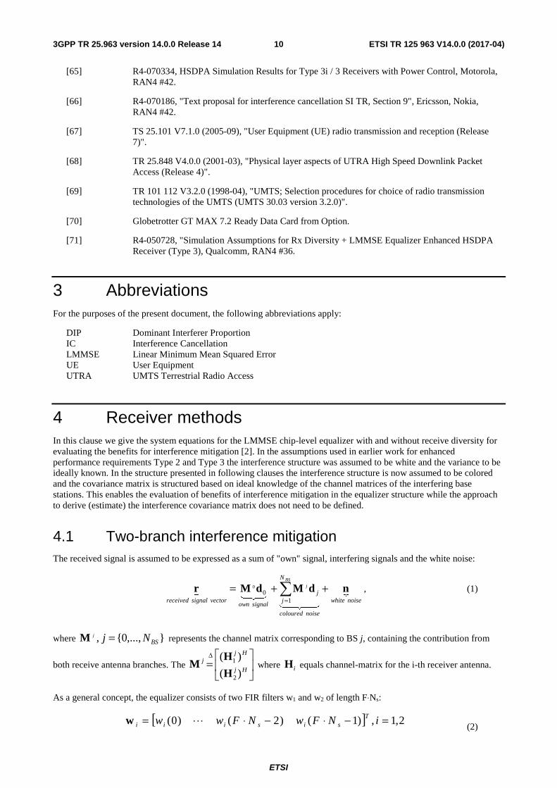
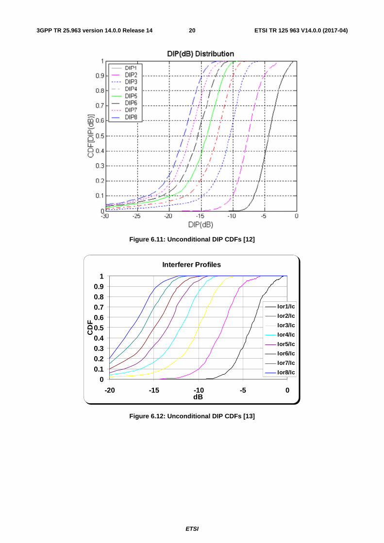
The group evaluated unconditional DIP values for the eight strongest interfering cells, as well as conditional DIP values conditioned on -3 dB, 0 dB, 5 dB, and 10 dB values of geometry. Figures 6.9 to 6.12 show CDFs of unconditional DIPi for the eight strongest interferers. Figures 6.13 to 6.15 show median values of conditional DIPi for different values of geometry. Based on these DIP results at that time the group decided that since there was not a large variability in DIP values for different geometries, the group could simplify the number of simulation scenarios by defining an interference profile with a single set of median DIP values for all geometries.

Median Interferer Ratios at Various Geometries

0

0.1

0.2

0.3

0.4

0.5

Ior1/Ic Ior2/Ic Ior3/Ic Ior4/Ic Ior5/Ic Ior6/Ic Ior7/Ic Ior8/Ic

Rat

ios

Geometry = -3 dB

Geometry = 0 dB

Geometry = 5 dB

Geometry = 10 dB

ETSI


Figure 6.9: Unconditional DIP CDFs [10]


ETSI




Interferer Profiles

00.10.20.30.40.50.60.70.80.9

1

-20 -15 -10 -5 0dB

CD

F

Ior1/Ic

Ior2/Ic

Ior3/Ic

Ior4/Ic

Ior5/Ic

Ior6/Ic

Ior7/Ic

Ior8/Ic

ETSI


Figure 6.13: Conditional Median DIPs [10]


-18

-16

-14

-12

-10

-8

-6

-4

-2

-3 dB 0 dB 5 dB 10 dB All

Med

ian

DIP

(dB

)

Geometry (Ior/Ioc)

DIP1 DIP2 DIP3 DIP4 DIP5

ETSI



Thus, an interference profile was defined on the basis of averaging unconditional median DIP values submitted by four companies as shown in Table 6.1. It was agreed [15] that the interference profile would consist of the averaged set of five median DIP values and one residual interferer to model the remaining interference. It was also agreed that the residual interferer would be modeled as filtered AWGN. Based on the DIP values shown in Table 6.1, the ratio AWGN/Ioc should be set to -5.8 dB, which is equivalent to about 26% of the total other cell interference power. The AWGN source should be filtered using the pulse shaping filter defined in TS 25.104 to insure correct spectral properties. These median DIP values plus the residual AWGN were to be used with each of the geometries considered in the initial link level characterization. The geometry values used in that initial characterization were -3 dB, 0 dB, 5 dB and 10 dB, see clause 8.

Table 6.1: Interference Profile Based on Averaged Set of Unconditional Median DIP Values [14]

Cingular Qualcomm Motorola Nokia Average

DIP1 -4.1 -4.1 -4.4 -4.4 -4.2

DIP2 -7.3 -7.3 -7.6 -8.0 -7.5

DIP3 -10.0 -10.0 -10.5 -11.5 -10.5

DIP4 -12.1 -12.0 -12.5 -14.0 -12.6

DIP5 -13.8 -13.6 -14.1 -17.0 -14.4

AWGN/Ioc -6.6 -6.7 -5.6 -4.6 -5.8

22% 21% 28% 35% 26%

6.3 Interference profiles based on weighted average throughput gain

6.3.0 General

Upon reviewing the initial link level performance results for the interference profile based on median DIP values, some companies expressed concern that these values were too conservative, and led to under-estimation of the benefits of IC receivers. This led to the development of an alternative method for calculating DIP values based on what is called the ‘weighted average throughput gain’ as described in [8]. This method develops multiple sets of DIP ratios, the resulting throughputs of which are averaged to find an average throughput gain. The set of DIP ratios closest to this average is then selected as the interference profile. Two profiles were ultimately defined, one for 0 dB geometry, and the other for

Median DIP Conditioned on Geometry

-20

-18

-16

-14

-12

-10

-8

-6

-4

-2

-3 dB 0 dB 5 dB 10 dB AllGeometry (Ior/Ioc)

Med

ian

DIP

(dB

)

DIP1 DIP2 DIP3 DIP4 DIP5 DIP6 DIP7 DIP8

ETSI


-3 dB geometry. The remainder of this clause describes the methodology used to define these two interference profiles along with their associated values. Note since the initial link level gains were negligible for the higher geometries (5 and 10 dB), the group agreed to focus on performance at the lower geometries, which is intuitively where an IC receiver is going to provide benefit.

6.3.1 0 dB geometry

The 0 dB geometry profile based on weighted average throughput gain was defined based on a methodology presented in [8] and explained further as follows. In the static system simulator, UEs were randomly placed throughout the simulated cells of interest. All of the randomly placed UEs with a geometry of near Ior1/Ioc = 0dB (±0.2 dB) were chosen and their DIP values were saved. This process was repeated for multiple realizations, until a significant number of samples were obtained. Then, the saved DIP values were sorted by DIP1 and then binned in 5-percentile bands. One random sample was drawn from each 5-percentile band to obtain a total of 20 representative DIP ratio sets. Table 6.2 shows the 20 representative DIP ratio sets that were used to define the interference profile for the 0 dB case.

Table 6.2: DIP ratios for Ior1/Ioc = 0dB [8]

# Ior1/Ioc DIP1 DIP2 DIP3 DIP4 DIP5 Ioc

1 -0.08 -8.22 -9.39 -9.99 -10.11 -10.73 -61.62

2 0.07 -6.35 -7.85 -8.09 -8.61 -9.47 -68.37

3 -0.01 -5.74 -6.41 -10.70 -11.19 -11.50 -54.74

4 0.05 -5.38 -7.48 -7.57 -7.68 -15.79 -60.59

5 -0.01 -4.94 -5.30 -8.05 -13.64 -14.11 -65.75

6 -0.09 -4.68 -5.73 -8.11 -12.38 -15.16 -57.44

7 -0.09 -4.40 -5.38 -8.73 -13.72 -13.80 -49.08

8 0.01 -4.14 -9.26 -10.12 -11.85 -13.54 -54.25

9 -0.06 -3.93 -8.89 -10.65 -11.50 -12.78 -65.95

10 0.09 -3.65 -7.36 -9.25 -12.49 -13.58 -63.34

11 0.02 -3.43 -8.55 -8.72 -11.52 -15.01 -63.50

12 -0.04 -3.17 -4.33 -14.32 -15.99 -18.96 -58.68

13 0.04 -3.00 -4.66 -13.34 -17.61 -20.61 -56.81

14 0.00 -2.75 -7.64 -8.68 -13.71 -14.59 -41.51

15 -0.05 -2.40 -4.99 -12.37 -18.32 -18.70 -47.09

16 -0.01 -2.12 -8.97 -9.13 -15.77 -17.90 -63.01

17 -0.03 -1.79 -11.42 -12.07 -14.54 -14.95 -65.39

18 0.04 -1.37 -9.47 -15.28 -16.42 -17.83 -69.25

19 0.07 -0.84 -14.86 -15.80 -16.01 -17.27 -51.90

20 0.08 -0.50 -11.39 -19.44 -21.55 -24.07 -53.99 Link level simulations were conducted for each of the above 20 representative sets of DIP ratios to obtain link level throughputs for each set. The average throughput gain over all 20 sets was then calculated. The DIP ratio set whose individual throughput gain was closest to the average throughput gain was then chosen as the DIP ratio set for the interference profile. For the data in Table 6.2, the DIP ratio set corresponding to row #14 was found to be the one with throughput gain closest to the average. The corresponding DIP values for this row are repeated in Table 6.3. These values were used in a second round of link level characterization for the 0 dB geometry case as described in clause 8.

Table 6.3 Interference Profile Based on Weighted Average Throughput for 0 dB Geometry [8]

DIP1 [dB] DIP2 [dB] DIP3 [dB] DIP4 [dB] DIP5 [dB] -2.75 -7.64 -8.68 -13.71 -14.59

6.3.2 -3 dB geometry

In the methodology used to define the interference profile for the 0 dB geometry case in clause 6.3.1 a random sample was drawn from each of the 20 5-percentile bins to obtain the 20 sets of representative DIP ratios. It was pointed out in [18] that due to this random draw, the interference profile defined in clause 6.3.1 was not repeatable by other companies. If repeatability is desired, an alternative method of obtaining 20 representative DIP ratio sets based on bin-

ETSI


averaging was proposed in [18]. According to this alternative method the DIP values calculated for each 5 percentile interval are based on the average of all of the values that fall within that bin. For example, for the Ior1/Ioc = -3 dB case, all UEs whose DIP1 value is equal to -3 dB (±0.2 dB) are sorted according to DIP1 and sampled at 5 percentile intervals to yield 20 groups. The 20 representative DIP values are the average of the DIP values observed by all UEs that fall within each of these 20 groups. The 20 sets of DIP values, calculated using the bin-averaging method for the -3 dB geometry case are shown in Table 6.4.

Table 6.4 DIP values for Ior/Ioc = -3 dB, sorted on 5th percentile increments. [19]

Bin # Ior/Ioc DIP1 DIP2 DIP3 DIP4 DIP5

1 -2.998 -6.937 -7.659 -8.454 -9.608 -10.972

2 -2.994 -6.135 -7.058 -8.320 -9.880 -11.729

3 -3.007 -5.755 -6.761 -8.203 -10.258 -12.123

4 -3.003 -5.481 -6.616 -8.414 -10.446 -12.231

5 -3.016 -5.238 -6.392 -8.339 -10.864 -12.762

6 -2.992 -5.043 -6.398 -8.617 -10.961 -12.975

7 -3.003 -4.866 -6.498 -8.647 -11.006 -12.908

8 -3.001 -4.697 -6.423 -8.928 -11.357 -13.136

9 -2.983 -4.524 -6.180 -8.960 -11.626 -13.544

10 -2.993 -4.370 -6.210 -9.245 -11.654 -13.750

11 -2.984 -4.218 -6.148 -9.594 -11.979 -13.862

12 -2.996 -4.088 -6.202 -9.508 -12.007 -14.064

13 -3.001 -3.959 -6.205 -9.537 -12.151 -14.229

14 -3.002 -3.830 -6.435 -10.064 -12.304 -13.839

15 -2.996 -3.699 -6.537 -9.879 -12.378 -14.146

16 -2.994 -3.556 -6.362 -10.123 -12.648 -14.409

17 -3.007 -3.423 -6.515 -10.314 -12.788 -14.436

18 -2.998 -3.300 -6.598 -10.454 -12.785 -14.702

19 -2.975 -3.174 -6.772 -10.619 -12.882 -14.717

20 -2.897 -3.003 -7.078 -10.791 -13.061 -14.689 It was shown in [18], that both the random draw and bin-averaging methods produce the same throughput gains for the 0 dB geometry case and thus, either method was deemed acceptable for this case. However, this was not found to be the case for the -3 dB geometry condition, where in [19] there was shown to be a significant difference between the throughput gains for the two methods. A significant difference was also observed in [20] where throughput gains were compared using just the random draw method. Based on all of this, the group decided [21] to adopt the alternative method based on bin-averaging for the -3 dB geometry case, but to leave the interference profile defined for the 0 dB case in clause 6.3.1 unchanged since there was no significant difference in link level throughput results for this latter case.

Applying the ‘weighted average throughput gain’ method to the data of Table 6.4 results in the selection of row #10 as the interference profile for the -3 dB geometry case. For clarity, the selected DIP values of row #10 are repeated in Table 6.5 below. Note in [19] the DIP ratio set is actually selected based on the weighted average throughput as opposed to the weighted average throughput gain, but the two methods were found to be nearly equivalent for the data analyzed, and in fact the former method gave a more consistent answer.

Table 6.5: Interference Profile based on Weighted Average Throughput for Ior1/Ioc = -3 dB [19]

DIP1 [dB] DIP2 [dB] DIP3 [dB] DIP4 [dB] DIP5 [dB] -4.37 -6.21 -9.25 -11.65 -13.75

6.4 Interference profiles based on field data The interference profiles defined in clauses 6.3 and 6.4 are all based on the use of static system level simulators. These simulators are based on a homogeneous layout of hexagonal cells with uniformly distributed users. Thus, they fail to capture a number of real-world effects including non-homogeneity of cells, buildings/terrain, and non-uniform distribution of users, just to name a few. Even with these shortcomings, system level simulations are still extremely

ETSI


valuable since the results developed are typically repeatable and one can precisely control the environment. However, it is also very important to consider actual field data when attempting to determine the feasibility of an advanced UE receiver that is attempting to cancel interference from other cells as is being considered in this study item. To this end, several contributions were submitted during this effort, which describe a number of field measurements [9] [22] [23] [24]. These measurements provide additional insight into how well an IC receiver might actually perform in a real network. In addition, interference profiles conditioned on geometry were defined based on one of the sets of field data. Link level characterization using this latter set is described in clause 8. The following briefly describes some of the main observations that can be drawn from the field data plus the specifics of the field-based interference profiles.

In [22] interference data collected in a live UMTS network in Paris is described. The major observations from these measurements are as follows:

- For mobiles at the cell edge, there are in general no more than 3 interfering cells seen by the UE. In about 65% of the time, there are only 2 interferers detected.

- DIP 1 values are fairly high (when compared to other DIP values) and not too spread out, ranging between 0 and -4 dB, at geometry Ior/Ioc = 0.

- DIP 2 and DIP 3 values are more spread out.

- There are not enough 4th interferers detected to include in a meaningful statistical analysis.

- A 3-D representation of data confirmed the spread of DIP 2 in particular over a large range of values: from -2dB to about -13 dB.

In [23] field measurements are provided for an operational UMTS/HSDPA network in parts of greater and downtown Chicago. The results from these measurements indicate that for the 0 dB geometry case that most of the interfering energy when measured at the median points of the DIP CDF curves is contained in the first two interfering cells (78%). For -3 dB geometry, most of the interfering energy is in the first three interfering cells (coincidentally 78%).

Field measurements of DIP values recorded in central London are presented in [24]. DIP measurements were taken conditioned on the following values of geometry: -3, 0, 5, and 10 dB. Based on these measurements, DIP profiles were defined as shown in Table 6.6. These values are based on taking the median value of each respective DIP value for each of the geometries considered. Even though this approach (taking the median value) is thought to be conservative, the values in Table 6.6 are still more optimistic from an IC performance perspective than the other profiles previously defined, see clause 6.6. If one were to apply the ‘weighted average throughput gain’ method to this field data, the results would be even more optimistic. Link level results based on the DIP ratios corresponding to -3 and 0 dB geometries are provided in clause 8.

One of the conclusions that can be drawn from all of the field measurements is that most of the interference is contained in the first two interfering cells with some energy in the third depending upon geometry. Very little energy was detected in the fourth and beyond, and thus, the use of five interfering cells in the simulation-based profiles may be bit of an over kill. The second conclusion is that field-based profiles are more optimistic than the simulation-based profiles and thus, performance in the real world (at least in those locations where the field data was collected) should be better than that predicted by the simulations.

Table 6.6: Interference Profiles Based on Field Data [24]

Îor1/Ioc DIPi -3dB 0dB 5dB 10dB DIP1 -4.1 -1.9 -1.8 -1.8 DIP2 -6.3 -8.7 -8.5 -9.4 DIP3 -9.1 -14.6 -15.8 -14.9 DIP4 -12.1 -20.6 -21.7 -20.2 DIP5 -15.3 -29.8 -31 -31

6.5 Summary In summary, Table 6.7 shows the interference profiles that have been defined as part of this feasibility study to assess link level performance of IC receivers. The top entry reflects the median DIP values, which are to be used for all geometries considered. The next entry defines the two DIP profiles that were defined based on the weighted average throughput gain method for the 0 dB and -3 dB geometries, respectively. The last entry shows the DIP entries based on field data where we have limited the geometries to 0 and -3 dB once since there is where gain for IC receivers is expected. It is interesting

ETSI


to note when comparing these profiles that the median profile is actually quite close to both of the profiles conditioned on -3 dB geometry, and how really close the latter two are to each other. This suggests that the median profile probably should have only been used for the -3 dB geometry condition, and that it is important to condition the DIP ratios on geometry to obtain meaningful results. Link level performance results based on these interference profiles are presented in clause 8.

Table 6.7: Summary of Defined Interference Profiles

Profile DIP1 DIP2 DIP3 DIP4 DIP5 Based on median values -4.2 -7.5 -10.5 -12.6 -14.4 Based on weighted average throughput gain

0 dB geometry -2.75 -7.64 -8.68 -13.71 -14.59 -3 dB geometry -4.37 -6.21 -9.25 -11.65 -13.75 Based on field data 0 dB geometry -1.9 -8.7 -14.6 -20.6 -29.8 -3 dB geometry -4.1 -6.3 -9.1 -12.1 -15.3

7 Transmitted code/power characteristics

7.0 General This clause describes the modelling methods and assumed characteristics of desired and interfering signals for this study.

7.1 Transmitted code and power characteristic in case of HSDPA

In the following clauses the modelling of code and power characteristics for serving and interfering cells is presented. The text is based on [29] aiming to merge the proposals presented in documents [25][26][27][28] accounting also the discussions held during RAN4#39. Also additional changes proposed in [30] and [31] were accounted as agreed in interim teleconference held between RAN4 meetings #41 and #42 [21].

For modelling the transmitted code and power domain characteristics in case of HSDPA, two difference scenarios are determined; the ‘HSDPA-only’ and ‘HSDPA+R’99’. The scenarios described in this clause are separated by the used HS-PDSCH power allocation and modelling of the associated dedicated channels. For ‘HSDPA-only’, 66% HS-PDSCH power allocation is assumed with associated channels modeled as F-DPCH, and for ‘HSDPA+R’99’ 50% and 25% allocations are assumed together with dedicated channels assumed as DPCH.

7.1.1 Common channels for serving and interfering cells

The common downlink channels and corresponding powers used in RAN4 HSDPA demodulation requirements with single transmit antenna are listed in the Table C.8 of TS25.101 [2]. Similar definitions exist also for open and closed loop transmit diversity requirements in Tables C.9 and C.10 in [2]. Table 7.1 below summarizes the common downlink physical channels for single transmit antenna case. As these figures can be considered to be quite representative, it is seen that these could be used also for the evaluation, for both, serving cell and interfering cells, in case of single transmit antenna.

ETSI


Table 7.1: Downlink Physical Channels transmitted during a connection for HSDPA

Physical Channel Power ratio NOTE

P-CPICH P-CPICH_Ec/Ior = -10 dB

Use of P-CPICH or S-CPICH as phase reference is specified for each requirement and is also set by higher layer signalling.

P-CCPCH P-CCPCH_Ec/Ior = -12 dB When BCH performance is tested the P-CCPCH_Ec/Ior is test dependent

SCH SCH_Ec/Ior = -12 dB This power shall be divided equally between Primary and Secondary Synchronous channels

PICH PICH_Ec/Ior = -15 dB

7.1.2 Serving cell

In this clause the definition of transmitted code and power characteristics are given for the serving cell.

7.1.2.1 Transmitted code and power characteristics for HSDPA+R’99 scenario

The assumed downlink physical channel code allocations for HSDPA+R’99 scenario is given in Table 7.2. Table 7.3 summarizes the power allocations of different channels for the serving cell in ‘HSDPA+R’99’ scenario for 50 % or 25 % HS-PDSCH power allocation.

Ten HS-PDSCH codes have been reserved for user of interest in Table 7.2. Depending on the used fixed reference channel definition, H-SET3 or H-SET6, part of these may be left unused.

In total 46 SF=128 codes have been reserved for other users channels (OCNS). For HSDPA+R’99 scenario the (associated) dedicated channels of other users are modeled as DPCH. The amount of users present is dependent on the power remaining available after HSDPA allocation. For HSDPA power allocation of 50%, 18 users were fitted to cell. Correspondingly with HSDPA allocation of 25%, 34 users were fitted to the cell. The definition of the other user orthogonal channels and channel powers are given in Table 7.4 and Table 7.5. Power control behavior of the other users is introduced as described in Clause 7.1.4.

Table 7.2: Downlink physical channel code allocation for HSDPA+R’99

Channelization Code at SF=128 Note 0, 1 P-CPICH, P-CCPCH and PICH on SF=256 2…7 6 SF=128 codes free for OCNS 8…87 10 HS-PDSCH codes at SF=16 88…127 40 SF=128 codes free for OCNS

Table 7.3: Summary of modelling approach for the serving cell in HSDPA+R’99 scenarios

Serving cell Common channels 0.195 (-7.1dB)

As given in Table 7.1 HS-PDSCH transport format H-SET3 or H-SET6 HS-PDSCH power allocation

[Ec/Ior] 0.5

(-3dB) 0.25

(-6dB) Other users channels 0.305

(-5.16dB) Set as given in Table 7.4

0.555 (-2.58dB)

Set as given in Table 7.5 NOTE: The values given in decibel are only for information.

ETSI


Table 7.4: Definition of 18 other users orthogonal channels on downlink scenario with 50% HS-PDSCH power allocation

Channelization Code Cch,SF,k

Ec/Ior Channelization Code Cch,SF,k


Ec/Ior

Cch,128,2 0.0204 Cch,128,98 0.0269 Cch,64,58 0.0294 Cch,128,4 0.0105 Cch,128,100 0.0170 Cch,128,121 0.0269 Cch,128,6 0.0115 Cch,128,102 0.0091 Cch,128,123 0.0204

Cch,128,88 0.0110 Cch,64,52 0.0232 Cch,128,125 0.0069 Cch,128,91 0.0112 Cch,128,109 0.0129 Cch,128,93 0.0110 Cch,128,111 0.0178 Cch,128,95 0.0316 Cch,128,114 0.0072

Table 7.5: Definition of 34 other users orthogonal channels on downlink scenario with 25% HS-PDSCH power allocation




Ec/Ior

Cch,128,2 0.0229 Cch,128,98 0.0129 Cch,128,114 0.0110 Cch,128,3 0.0182 Cch,128,99 0.0162 Cch,128,115 0.0110 Cch,128,4 0.0076 Cch,128,100 0.0170 Cch,128,116 0.0110 Cch,128,5 0.0155 Cch,128,101 0.0102 Cch,128,118 0.0316 Cch,128,6 0.0245 Cch,128,103 0.0182 Cch,128,119 0.0269 Cch,64,44 0.0304 Cch,64,52 0.0379 Cch,64,60 0.0261 Cch,128,90 0.0081 Cch,128,106 0.0132 Cch,128,123 0.0120 Cch,128,91 0.0065 Cch,128,108 0.0229 Cch,128,124 0.0115 Cch,128,93 0.0069 Cch,128,109 0.0145 Cch,128,125 0.0132 Cch,128,94 0.0110 Cch,128,110 0.0115 Cch,128,126 0.0110 Cch,128,95 0.0135 Cch,128,111 0.0200 Cch,128,96 0.0200 Cch,128,113 0.0102

7.1.2.2 Transmitted code and power characteristics for HSDPA-only scenario

The assumed downlink physical channel code allocations for the HSDPA-only scenario is given in Table 7.6. In the Table 7.7 power allocations for the serving cell is presented for HSDPA-only scenario.

For HSDPA-only scenario, as in Table 7.6, 14 codes are made available for the HS-DSCH as all the associated dedicated channels use F-DPCH. Depending on the used fixed reference channel definition, H-SET3 or H-SET6, part of these may be left unused. In order to permit comparable simulations to be performed using existing FRC definitions, an additional code multiplexed user is introduced to the serving cell of HSDPA-only scenario. As H-SET6 requires a maximum of 10 codes and H-SET3 requires 5 codes, additional code multiplexed user is defined in case of the serving cell. This additional code multiplexed user utilizes the rest of the available codes assumed to be available for HSDPA. The code channels intended for the additional code multiplexed user shall have equal power and common modulation. The power per code for H-SET6 shall be either 0.04 (-14 dB) when HS-DSCH Ec/Ior allocated for the DUT is 50%, or 0.1025 (-9.9 dB) when HS-DSCH Ec/Ior allocated for the DUT is 25%. The respective per code power allocations for H-SET3 are 0.01777 (-17.5 dB) and 0.04555 (-13.4 dB), see Tables 7.8 and 7.9. Used common modulation (QPSK or 16QAM) should be randomly selected with equal probability.

The definition of other users orthogonal channels is given in Table 7.10. The channelization code indices, Cch,256,x and Cch,256,y given at same row are considered as pair. At any given symbol instant, only symbol from either code channel is transmitted with the Ec/Ior given in the last column of the same row. The other code channel is DTX’ed. The code channel transmitted is selected randomly with even probability. This is done to account the structure of the F-DPCH.

Table 7.6: Downlink physical channel code allocation for HSDPA-only scenario

Channelization Code at SF=128

Note

0 P-CPICH, P-CCPCH and PICH on SF=256 1

2…7 6 SF=128 codes free for OCNS 8…119 14 HS-PDSCH codes at SF=16

120…127 8 SF=128 codes free for OCNS

ETSI


Table 7.7: Summary of the modelling approach for the serving cell in HSDPA-only scenarios

Serving cell Common channels 0.195 (-7.1dB)

As given in Table 7.1 HS-PDSCH transport format H-SET3 or H-SET6 for user of interest.

Additional other HSDPA users code allocation is based on Table 7.8 for H-

SET3 or Table 7.9 for H-SET6. Total HS-PDSCH power allocation [Ec/Ior] 0.66

(-1.8dB) HS-PDSCH power allocation for DUT (of the total) [Ec/Ior]

[0.5, 0.25] ([-3dB, -6dB])

Other users dedicated channels 0.14 (-8.54dB)

Set according to Table 7.10. NOTE: The values given in decibel are only for information.

Table 7.8: Definition of additional code multiplexed users orthogonal channel for HSDPA-only scenario (H-SET3)


Ec/Ior [dB] Channelization Code Cch,SF,k


Ec/Ior [dB]

Cch,16,6 Note1 Cch,16,7 Note1 Cch,16,8 Note1 Cch,16,9 Note1 Cch,16,10 Note1 Cch,16,11 Note1

Cch,16,12 Note1 Cch,16,13 Note1 Cch,16,14 Note1 NOTE 1: Used common modulation should be randomly selected for codes with equal probability. The

code channels shall have equal power, either 0.01777 (-17.5 dB) when HS-DSCH Ec/Ior allocated for the DUT is -3dB or 0.04555 (-13.4 dB) when HS-DSCH Ec/Ior allocated for the DUT is -6dB.

Table 7.9: Definition of additional code multiplexed users orthogonal channel for HSDPA-only scenario (H-SET6)




Ec/Ior [dB]

Cch,16,11 Note2 Cch,16,12 Note2 Cch,16,13 Note2 Cch,16,14 Note2

NOTE 2: Used common modulation should be randomly selected for codes with equal probability. The code channels shall have equal power, either 0.04 (-14 dB) when HS-DSCH Ec/Ior allocated for the DUT is -3dB or 0.1025 (-9.9 dB) when HS-DSCH Ec/Ior allocated for the DUT is -6dB.

Table 7.10: Definition of other users orthogonal channels on downlink for HSDPA-only scenario

Channelization Code Cch,SF,x

Channelization Code Cch,SF,y

Ec/Ior

Cch,256,4 Cch,256,243 0.0135 Cch,256,5 Cch,256,244 0.0200

Cch,256,249 Cch,256,246 0.0129 Cch,245,8 Cch,256,247 0.0166 Cch,256,9 Cch,256,6 0.0170

Cch,256,11 Cch,256,250 0.0102 Cch,256,240 Cch,256,253 0.0182 Cch,256,242 Cch,256,255 0.0316

7.1.3 Interfering cells

In this clause the definition of transmitted code and power characteristics are given for the interfering cells.

7.1.3.1 Transmitted code and power characteristics for HSDPA+R’99 scenario

For the interfering cells in HSDPA+R’99 scenario, same downlink physical channel code allocations are assumed as given in Table 7.2. The modelling is summarized in Table 7.11 for HSDPA+R’99 scenario for interfering cells.

ETSI


Table 7.11: Summary of modelling approach for the interfering cells in HSDPA+R’99 scenarios with power allocation of 50% and 25%

Interfering cell(s) Common channels 0.195 (-7.1dB)

As given in Table 7.1 HS-PDSCH transport format

Selected randomly from Table 7.12. Independent for each interferer.

HS-PDSCH power allocation [Ec/Ior]

0.5 (-3dB)

Other users channels 0.305 (-5.16dB)

Set according to Table 7.4. NOTE: The values given in decibel are only for information.

The HS-PDSCH transmission for interfering cells is modelled to have randomly varying modulation and number of codes to model the actual dynamic system behaviour to some extent. The predefined modulation and code allocations are given in Table 7.12. The transmission from each interfering cell is randomly and independently selected every HSDPA sub-TTI among the four options given in the table.

Table 7.12: Predefined interferer transmission for HSDPA+R’99 scenario

# Used modulation and number of HS-PDSCH codes

1 QPSK with 5 codes 2 16QAM with 5 codes 3 QPSK with 10 codes 4 16QAM, with 10 codes

The modelling of the other users dedicated channels is done in same way as in the case of the serving cell. The definition of the other users’ orthogonal channels and channel powers are given in Table 7.4. As fixed HSDPA power allocation (50%) is assumed for interfering cells, only one definition set is enough.

7.1.3.2 Transmitted code and power characteristics for HSDPA-only scenario

Same downlink physical channel code allocations as for serving cell, given Table 7.6, are used for the interfering cells in HSDPA-only scenario. The modelling of the transmission of the interfering cells for HSDPA-only scenario is summarized in Table 7.13.

Table 7.13: Summary of modelling approach for the interfering cells in HSDPA-only scenarios

Interfering cell(s) Common channels 0.195 (-7.1dB)

As given in Table 7.1 HS-PDSCH transport

format Selected randomly from Table 7.14.

Independent for each interferer. Total HS-PDSCH power

allocation [Ec/Ior] 0.66

(-1.8dB) Other users channels 0.14

(-8.54 dB) Set according to the Table 7.10

Note: The values given in decibel are only for information. Similarly as in case of HSDPA+R’99 scenario the HS-PDSCH transmission is modeled as having varying modulation and allocation of codes. This is done by selecting a code and modulation format from a group of predefined sets, as given in Table 7.14. Three different options are determined, with one option including code multiplexing. In case of the code multiplexing for the interfering HS-DSCH transmission (e.g. option #3) the power is divided equally between the two assumed users having different modulation.

ETSI


Table 7.14: Predefined interferer transmission for HSDPA-only scenario

# Used modulation and number of HS-PDSCH codes

1 QPSK with 14 codes 2 16QAM, with 14 codes 3 QPSK with 7 codes and 16QAM with 7 codes

7.1.4 Model for the power control sequence generation

In this clause the modelling of power control behavior for the other users channels is given. In the assumed approach

the power of each user, i at slot n, equals inP in dB. The power is varied randomly, either by increasing or decreasing it

by 1dB steps in each slot, i.e. Δ+= −i

ni

n PP 1 , where { }1,1 +−∈Δ . The probability of Δ having a value of +1 for the

ith user at time instant n can be determined as

L

PP iin

in

5.0)(5.0)1(Pr 01 −−=+=Δ − , (1)

where, inP 1− is the transmitted power at time instant n-1 and iP0 is the initial value of the ith users power in dB. The

initial transmit power values iP0 for different users are given in Tables 7.4 and 7.5 in absolute values. L is a scaling

factor which can be used to determine the range to which the variation of power is confined. The value of L is set to 10, leading to variance of 5 dB.

In order to minimize the impact to test equipment due to power control modelling the total OCNS power is intended to be normalized. Thus the power control sequence for each user is generated as described above. The actual applied

transmit power inP̂ (in linear domain) for the ith user would still be normalized by the total sum power of different

users, defined as

∑∑

=i

ilin

i

inlin

inlini

n PP

PP 0,

,

,ˆ . (2)

where ,ilin nP is the transmitted power at time instant n and ,0

ilinP is the initial value of the ith user’s power in linear

domain. The normalization has implications to the power variation of each user.

8 Link performance characterization

8.0 General The purpose of this clause is to summarize the link-level simulation results that were provided by the companies that supported this study item. Emphasis is on results that were based on agreed set of simulation parameters. However, a complete list of results is given in the appendix of this clause.

8.1 Overview This overview is meant to be a brief synopsis of the framework in which link-level simulations were performed. More detailed information regarding such topics as code modelling, system scenarios, and interference modelling are available elsewhere in this report. As described in clause 6 system simulations were performed by participating companies in order to reach an agreement on link-level simulation parameters. The main focus of this work was determining the number of interfering Node-Bs and associated set of DIP values and geometries to be used. Based on these simulation studies it was decided to set the number of interfering Node-Bs to five. Also, a single set of median DIP values would be used for selected geometries. See Table 8.1 for these and other referenced DIP values. In the

ETSI


course of this study it was proposed that median DIP values might give a pessimistic assessment of the potential gain that a LMMSE receiver with interference cancellation capability might provide. It was decided that the DIP values should be modified to take into account the potential gains at low geometries. Consequently a 2nd set of DIP values were accepted for link-level simulation purposes. In this case the DIP values are a function of the operating geometry; 0 or -3 dB. Afterwards, there was discussion regarding the method of generation of these DIP values. Subsequently it was decided to accept a modified DIP for geometry -3 dB. Contributions that investigated the DIP issue based on field measurements were also presented; simulations using these derived values were presented.

Table 8.1: DIP values (dB) used during progression of SI

Evolution DIP1 DIP2 DIP3 DIP4 DIP5 Status Median -4.2 -7.5 -10.5 -12.6 -14.4 Obsolete Weighted G=0 -2.75 -7.64 -8.68 -13.71 -14.59 Active Weighted G=-3 -3.21 -5.56 -10.01 -12.67 -15.53 Obsolete Revised Weighted G=-3 -4.37 -6.21 -9.25 -11.65 -13.75 Active Field Measurement G=0 -1.9 -8.7 -14.6 -20.6 -29.8 Information Field Measurement G=-3 -4.1 -6.3 -9.1 -12.1 -15.3 Information

8.2 Simulation results The following clauses 8.2.1 - 8.2.3 show the average relative gains as demonstrated by a type 2i over a type 2 receiver or a type 3i over a type 3 receiver. (As noted in clause 8.2.1, it was eventually decided that this SI would concentrate on the type 3 / 3i configuration. However, the type 2 / 2i results are given for completeness; similarly like simulation results for the obsolete DIP sets.) For a given simulation condition, average relative gain is defined as the ratio of the FRC throughput of the type 2i or 3i receiver to the throughput of the type 2 or 3 receiver, respectively. This "normalized" numerical result allows for a readily discernable evaluation of the efficacy of the type 2i / 3i receiver. However, this single quantity may not tell the complete story. If for example, the relative gain for a given channel condition is shown to be 7.0 for a 16QAM configuration, while the relative gain is 1.3 for QPSK under the same condition, the utility of the 16QAM value is of little practical importance if the actual throughput values are 7 Kb/s and 1 Kb/s for the type i and non type i receivers. Whereas, if for the same channel condition the QPSK throughput values are 195 Kb/s and 150 Kb/s for the different receivers, these values might be considered substantial and useful gains. Therefore, the corresponding average FRC throughput values are shown - expressed as ratio of integers - for all relative gains2.

8.2.1 Types 2 and 2i - median DIP values

Tables 8.2 and 8.3 show the relative average gains and throughputs of the type 2i / 2 receivers for the various signal levels and channel conditions as indicated for the HSet-6 HSDPA+R99 QPSK and 16QAM scenarios, respectively. These sets of statistics are based on the contributions of six companies; see Appendix, Tables 8.A1 - 8.A23

Table 8.2: HSet-6 QPSK gains and throughputs for types 2i / 2 receivers for HSDPA+R99 with median DIP values

QPSK HSet6 PB3 VA30 Signal Level Ec/Ior (dB)

G (dB) G(dB) G (dB) G (dB) G (dB) G (dB) 0 5 10 0 5 10

-6 1.22 179 / 146

1.04 973 / 933

1.01 1645 / 1635

1.44 130 / 91

1.05 1040 / 992

1.01 1707 / 1693

-3 1.08 785 / 728

1.03 1626 / 1583

1.00 2594 / 2587

1.10 838 / 764

1.02 1636 / 1600

1.00 2505 / 2493

2 It should be noted that the relative gains and ratio of throughput values may not be equal. This is due to the fact that average of a set of ratios, is not equal to the average of the numerators divided by the average of the denominators.

3 Due to the nature of this section, where a considerable number of contributions are condensed into a single statistic, direct reference is not made to the contribution(s). Rather, the “raw data” of the contributions are given in a set of tables in the appendix; the tables give the RAN4 TD numbers for the individual values, this TD may be cross-referenced in the Reference section for the complete title and date.

ETSI


Table 8.3: HSet-6 16 QAM gains and throughputs for types 2i / 2 receivers for HSDPA+R99 with median DIP values

16QAM HSet6 PB3 VA30 Signal Level Ec/Ior (dB)


-6 2.03 7 / 5

1.09 394 / 362

1.01 1375 / 1363

1.00 1 / 1

1.19 373 / 312

1.02 1560 / 1490

-3 1.22 247/202

1.04 1355 / 1303

1.01 2188 / 2176

1.30 166 / 132

1.04 1422 / 1360

1.01 2288 / 2260

Tables 8.4 and 8.5 give simulation results similar to above but for HSet-3. In this case the statistics are based on two contributing companies; see Appendix, Table 8.A4 and 8.A5.

Table 8.4: HSet-3 QPSK gains and throughputs for types 2i / 2 receiver for HSDPA+R99 with median DIP values



-6 1.06 407 / 382

1.02 809 / 825

0.99 1301 / 1311

1.06 435 / 410

1.01 735 / 728

1.00 1277 / 1270

-3 1.04 738 / 712

1.01 1305 / 1294

0.96 1520 / 1579

1.03 732 / 712

1.00 1097 / 1094

1.00 1546 / 1546

Table 8.5: HSet-3 16QAM Gains and throughputs for types 2i / 2 receiver for HSDPA+R99 with median DIP values



-6 1.23 146 / 120

1.02 725 / 712

1.01 1150 / 1138

1.46 127 / 89

1.05 770 / 735

1.01 1217 / 1200

-3 1.07 599 / 562

1.02 1124 / 1104

1.01 1724 / 1707

1.07 618 / 576

1.02 1148 / 1127

1.01 1795 / 1682

From the above tables it can be observed that for geometries of 5 or 10 dB the gains are generally small, with all gains less than 1.10 except for one case where the gain is 1.19. The average of the gains for geometries 5 and 10 dB is 1.02. This average is based on all modulation types, signal levels, channels, and scenarios. The average relative gain for geometry 0 dB is 1.10 when the average is computed only over the better performing modulation scheme for a given channel and signal level; this is always QPSK in these cases.

8.2.2 Types 3 and 3i - median DIP values

Tables 8.6 and 8.7 give the relative gains and absolute ratios for receiver types 3 and 3i for HSet-6 and the indicated modulation with the use of the median DIP values. These statistics are based on appendix Tables 8.A10 and 8.A11.

Table 8.6: HSet-6 QPSK gains and throughputs for types 3i / 3 receivers for HSDPA+R99 with median DIP values



-6 1.16 1001/861

1.04 1865 / 1790

1.00 3005 / 2994

1.15 1042 / 908

1.05 1845 / 1759

1.01 2880 / 2850

-3 1.09 1630 / 1490

1.03 2941 / 2854

1.00 3218 / 3217

1.09 1619 / 1485

1.04 2771 / 2660

1.00 3212 /3209

ETSI


Table 8.7: HSet-6 16QAM gains and throughputs for types 3i / 3 receivers for HSDPA+R99 with median DIP values



-6 1.66 360 / 217

1.05 1643 / 1560

1.03 2541 / 2469

2.41 311 / 128

1.06 1673 / 1577

1.02 2530 / 2466

-3 1.16 1393 / 1201

1.03 2384 / 2303

1.01 3915 / 3862

1.17 1436 / 1230

1.04 2409 / 2320

1.02 3676 / 3607

From the tables for types 3i and 3 receivers simulated under the median DIP set, the average gain computed over geometries 5 and 10 dB is 1.03. Based on these results, including the type 2i / 2 receivers, it was decided to limit the study item to lower geometries, specifically -3 and 0 dB.

The average relative gain for geometry 0 dB is 1.13 when the average is computed only over the better performing modulation scheme for a given channel and signal level; like the types 2i / 2 case, this is for QPSK modulation. It was decided that only the type 3i / 3 case would be further studied. This decision was not based solely on the gain of 1.13 of the type 3i / 3 compared to the 1.10 gain of the type 2i / 2, as the performance gains are somewhat comparable. However, when the absolute throughput values at geometry 0 dB are compared for both receiver groups, the larger throughputs of the 3i receiver influenced the decision to limit the study item to the 3i / 3 case.

8.2.3 Weighted DIPS: geometries -3 & 0 dB

As indicated in the Overview of this clause the study group decided to use a set of weighted DIP values rather than median DIP values in order to more realistically determine the potential gain of the type 3i receiver under low geometry conditions. Tables 8.8 and 8.9 show the results when these weighted DIPs were used for simulation. In this case these tables represent the combined results of the HSDPA+R99 and HSDPA only scenarios. Specifically, there were 6 independent contributions for the HSDPA+R99 scenario, and 2 to 4 independent contributions, dependent upon the channel condition and geometry, for the HSDPA only scenario. In order to maximize the number of samples for averaging the results of both scenarios were combined. However, if a company contributed to HSDPA+R99 and HSDPA scenario, then just the HSDPA only scenario was used in the averaging. Because of the very close values for HSDPA+R99 and HSDPA only scenarios as observed when a given company submitted for both sets - this and prior simulations - it is believed that this is valid statistic. See appendix Tables 8.A16 through 8.A21

Tables 8.8 and 8.9 show the substantial relative gain that a type 3i receiver may realize over a type 3 at the low geometries of 0 and -3 dB. Also, it should be noted that these gains are at very useful throughput values. Again QPSK shows the better performance, though at geometry 0 dB and Ec/Ior = -3 dB, the difference between QPSK and 16QAM is fairly close.

Table 8.8: HSet-6 QPSK gains and throughputs for types 3i / 3 receivers with weighted DIP values


G (dB) G (dB) G (dB) G (dB) -3 0 -3 0

-6 2.79 508 / 209

1.32 1113 / 852

3.81 618 / 177

1.30 1171 / 904

-3 1.38 1224 / 894

1.18 1780 / 1509

1.31 1292 / 983

1.20 1805 / 1498

Table 8.9: HSet-6 16QAM gains and throughputs for types 3i / 3 receivers with weighted DIP values


G (dB) G (dB) G (dB) G (dB) -3 0 -3 0

-6 5.46 34 / 7

2.51 439 / 189

30.50 16 /1

4.54 480 / 106

-3 2.58 721 / 297

1.32 1516 / 1147

4.14 837 / 229

1.30 1590 / 1225

ETSI


8.2.4 Revised DIP: geometry -3 dB

As discussed in Clause 6.3.2 it was decided to use a revised weighted DIP value for geometry -3 dB. Tables 8.10 and 8.11 show the average throughput and gain values based on the contributions that incorporated this modified DIP set. Again, these statistics are based on a combined set of HSDPA and HSDPA+R99 results. These simulations also include the modified set of OCNS codes that were concurrently agreed to when the revised DIP for geometry -3 dB was established. The tables show that for geometry -3 dB there is a small reduction in the average relative gains due to the revised DIP; compare to Tables 8.8 and 8.9.Whereas for a geometry of 0 dB there is a lesser degradation in the gains, especially for the QPSK values which tend to represent the more useful modulation scheme for these signal levels and geometries. (Only at geometry 0 dB and Ec/Ior = - 3 dB does 16QAM approach the QPSK average throughput values.) Because the DIP value was not changed for 0 dB it is to be expected that there should be little change in the prior results as shown in Tables 8.8 and 8.9 compared to those of 8.10 and 8.11 at 0 dB. Probably most of the change is due to the sample size for geometry 0 dB. In this case there were only 3 and 2 sets of independent simulation results for PB3 and VA30, respectively. Whereas for geometry - 3 dB there are 7 and 6 sets for PB3 and VA30. See appendix Tables 8.A22 - 8.A31 for the complete set of simulation results, which include similar contributions for H-Set 3.

Table 8.10: HSet-6 QPSK gains and throughputs for types 3i / 3 receivers with revised DIP values


G (dB) G (dB) G (dB) G (dB) -3 0 -3 0

-6 2.05 406 / 201

1.36 1216 / 889

3.02 409 / 142

1.30 1177 / 911

-3 1.24 1159 / 932

1.20 1857 / 1542

1.22 1175 / 964

1.20 1811 / 1514

Table 8.11: HSet-6 16QAM gains and throughputs for types 3i / 3 receivers with revised DIP values


G (dB) G (dB) G (dB) G (dB) -3 0 -3 0

-6 3.98 20 / 5

2.18 570 / 262

5.00 4 / 1

4.14 571 / 144

-3 2.01 537 / 269

1.31 1641 / 1239

3.15 567 / 185

1.29 1613 / 1254

8.2.5 Power control

As explained in Clause 7 it was decided to investigate two methods to model the effects of power control. These two methods are referred to "normalized" and "un-normalized" power control. Based on the contributions by participating companies the simulation results showed that power control had relatively little effect on the average throughput and relative gains; see appendix Table 8.A32 - 8.A39, For example, based on appendix Table 8.A32, for H-Set 6 QPSK HSDPA+R99 scenario with geometry -3 dB and propagation channel PB3 the average un-normalized throughput relative to no power control was 0.93, and for normalized it was 1.04. For the same conditions for geometry 0 dB the relative un-normalized throughput is 0.97, while the normalized is 1.00. Note: this is based on only two independent sets of simulation results, but there is a strong similar consistency throughout the submitted data4. Consequently the relative throughput gains due to interference cancellation are only negligibly modified by power control. This is due to the structure of the reference receiver, the LMMSE. This statement of course may not hold in general when other types of receivers may be subjected to power controlled signals. Finally, it is reasonable to conjecture that the un-normalized power control induces instances of larger interference compared to the normalized power control. Therefore, there is somewhat greater degradation due to un-normalized power control.

8.2.6 Field based DIP

As outlined in clause 6.4 there were contributions addressing the modelling of DIP values based on field measurements. Subsequently, simulation results utilizing these field measurements were contributed. Table 8.1 gives the DIP sets for geometries 0 and -3 dB based on certain field measurements. Tables 8.12 and 8.13 give the simulated average throughput and relative gains for the stated conditions using these DIP values. The relative gain results for the QPSK H-

4 The reason for the small sample size of averaged data is due to the lack of multiple data sets that share the same set of conditions.

ETSI


Set 6 in Table 8.12 are within 15% or less of the similar values for the weighted revised DIP values shown in Table 8:10. The same comment is true regarding the corresponding 16QAM values shown in Tables 8.13 and 8.11. The results in this clause are based on appendix Tables 8.A40 and 8.A41.

Table 8.12: QPSK gains and throughputs for types 3i / 3 receivers with field based DIP values for propagation channel PB3 and HSDPA only scenario

QPSK H-Set 6 H-Set 3 Signal Level Ec/Ior (dB)

G (dB) G (dB) G (dB) G (dB) -3 0 -3 0

-6 2.33 511 / 220

1.50 1388 / 928

1.31 675 / 514

1.28 1033 / 808

-3 1.31 1331 / 1013

1.26 2030 / 1608

1.16 954 / 821

1.24 1505 / 1217

Table 8.13: 16QAM gains and throughputs for types 3i / 3 receivers with field based DIP values for propagation channel PB3 and HSDPA only scenario

16QAM H-Set 6 H-Set 3 Signal Level Ec/Ior (dB)

G (dB) G (dB) 0 0

-6 NA

1.38 939 / 678

-3 1.41 1855 / 1313

1.24 1346 / 1085

8.2.7 Types 2i / 2 receivers: weighted & revised DIPS

As this SI progressed there was a group decision to limit this SI to types 3i and 3 receivers [R4-061080]. However, there was one set of simulation results that reported throughput values and relative gains for types 2i / 2 receivers using the revised DIP for geometry -3 dB, and the weighted DIP for geometry 0 dB. Tables 8.14 and 8.15 show the results for H-Set 6 under the stated conditions. A comparison of these tables with Tables 8.10 and 8.11 show similar relative gains for conditions that lead to non-negligible throughput values; that is primarily corresponding to QPSK and Ec/Ior = - 3dB conditions. See appendix Tables 8.A42 - 8.A45 for the complete set of data.

Table 8.14: HSet-6 QPSK gains and throughputs for types 2i / 2 receivers with revised DIP values


G (dB) G (dB) G (dB) G (dB) -3 0 -3 0

-6

1.55 17 / 11

1.97 333 / 169

4.00 4 / 1

2.79 243 / 87

-3 1.36 367 / 269

1.33 942 / 707

1.64 275 / 168

1.35 1023 / 757

Table 8.15: HSet-6 16QAM gains and throughputs for types 2i / 2 receivers with revised DIP values


G (dB) G (dB) G (dB) G (dB) -3 0 -3 0

-6 NA 0 / 0

1.69 22 / 13

NA 0 / 0

NA 1 / 0

-3 1.06 17 / 16

1.98 441 / 223

NA 3 / 0

2.98 295 / 99

8.3 Appendix The tables contained in this appendix represent the totality of the simulations results contributed by the participating parties. It also shows the values that were used for computing the statistics in clauses 8.2. The following tables are contained herein:

Table 8.A1 Type 2i / 2, HSDPA + R99, PB3, H-Set6, Median DIP Table 8.A2 Type 2i / 2, HSDPA + R99, VA30, H-Set 6, Median DIP

ETSI


Table 8.A3 Type 2i / 2, HSDPA + R99, PA3, H-Set 6, Median DIP Table 8.A4 Type 2i / 2, HSDPA + R99, PB3, H-Set 3, Median DIP Table 8.A5 Type 2i / 2, HSDPA + R99, VA30, H-Set 3, Median DIP Table 8.A6 Type 2i / 2, HSDPA + R99, PA3, H-Set 3, Median DIP Table 8.A7 Type 3i / 3, HSDPA + R99, PB3, H-Set 3, Median DIP Table 8.A8 Type 3i / 3, HSDPA + R99, VA30, H-Set 3, Median DIP Table 8.A9 Type 3i / 3, HSDPA + R99, PA3, H-Set 3, Median DIP Table 8.A10 Type 3i / 3, HSDPA + R99, PB3, H-Set 6, Median DIP Table 8.A11 Type 3i / 3, HSDPA + R99, VA30, H-Set 6, Median DIP Table 8.A12 Type 3i / 3, HSDPA + R99, PA3, H-Set 6, Median DIP Table 8.A13 Type 3i / 3, HSDPA only, PB3, H-Set 6, Median DIP Table 8.A14 Type 3i / 3, HSDPA only, VA30, H-Set 6, Median DIP Table 8.A15 Type 3i / 3, HSDPA only, PB3, H-Set 3, Median DIP Table 8.A16 Type 3i / 3, HSDPA + R99, PB3, H-Set 6, Weighted DIPS Table 8.A17 Type 3i / 3, HSDPA + R99, VA30, H-Set 6, Weighted DIPS Table 8.A18 Type 3i / 3, HSDPA, PB3, H-Set 6, Weighted DIPS Table 8.A19 Type 3i / 3, HSDPA, VA30, H-Set 6, Weighted DIPS Table 8.A20 Type 3i / 3, Combined HSDPA & HSDPA+R99 PB3, H-Set 6, Weighted DIPS Table 8.A21 Type 3i / 3, Combined HSDPA & HSDPA+R99, VA30, H-Set 6, Weighted DIPS Table 8.A22 Type 3i / 3, HSDPA + R99, PB3, H-Set 6, Revised G= -3 DIP & Codes Table 8.A23 Type 3i / 3, HSDPA + R99, VA30, H-Set 6, Revised G= -3 DIP & Codes Table 8.A24 Type 3i / 3, HSDPA + R99, PB3, H-Set 3, Revised G= -3 DIP & Codes Table 8.A25 Type 3i / 3, HSDPA + R99, VA30, H-Set 3, Revised G= -3 DIP & Codes Table 8.A26 Type 3i / 3, HSDPA only, PB3, H-Set 6, Revised G= -3 DIP & Codes Table 8.A27 Type 3i / 3, HSDPA only, VA30, H-Set 6, Revised G= -3 DIP & Codes Table 8.A28 Type 3i / 3, HSDPA only, PB3, H-Set 3, Revised G= -3 DIP & Codes Table 8.A29 Type 3i / 3, HSDPA only, VA30, H-Set 3, Revised G= -3 DIP & Codes Table 8.A30 Type 3i / 3, Combined HSDPA & HSDPA + R99, PB3, H-Set 6, Revised G= -3 DIP & Codes Table 8.A31 Type 3i / 3, Combined HSDPA & HSDPA + R99, VA30, H-Set 6, Revised G= -3 DIP & Codes Table 8.A32 Type 3i / 3, HSDPA + R99, PB3, H-Set 6, Revised G= -3 DIP & Codes with Power Control Table 8.A33 Type 3i / 3, HSDPA + R99, VA30, H-Set 6, Revised G= -3 DIP & Codes with Power Control Table 8.A34 Type 3i / 3, HSDPA + R99, PB3, H-Set 3, Revised G= -3 DIP & Codes with Power Control Table 8.A35 Type 3i / 3, HSDPA + R99, VA30, H-Set 3, Revised G= -3 DIP & Codes with Power Control Table 8.A36 Type 3i / 3, HSDPA only, PB3, H-Set 6, Revised G= -3 DIP & Codes with Unnormalized Power

Control Table 8.A37 Type 3i / 3, HSDPA only, VA30, H-Set 6, Revised G= -3 DIP & Codes with Power Control Table 8.A38 Type 3i / 3, HSDPA only, PB3, H-Set 3, Revised G= -3 DIP & Codes with Power Control Table 8.A39 Type 3i / 3, HSDPA only, VA30, H-Set 3, Revised G= -3 DIP & Codes with Power Control Table 8.A40 Type 3i / 3, HSDPA only, PB3, H-Set 6, Field Derived DIP Values Table 8.A41 Type 3i / 3, HSDPA only, PB3, H-Set 3, Field Derived DIP Values Table 8.A42 Type 2i / 2, HSDPA+R99, PB3, H-Set 6, Revised G= -3 DIP & Codes Table 8.A43 Type 2i / 2, HSDPA+R99, VA30, H-Set 6, Revised G= -3 DIP & Codes Table 8.A44 Type 2i / 2, HSDPA+R99, PB3, H-Set 3, Revised G= -3 DIP & Codes Table 8.A45 Type 2i / 2, HSDPA+R99, VA30, H-Set 3, Revised G= -3 DIP & Codes

ETSI


Table 8.A1: Type 2i / 2, HSDPA + R99, PB3, H-Set6, Median DIP

Rx Type 2 2 2i 2i 2 2 2i 2i Gain Gain Gain Gain Reference

Modulation QPSK QPSK QPSK QPSK 16QAM 16QAM 16QAM 16QAM QPSK QPSK 16QAM 16QAM

Ec/Ior (dB) -6 -3 -6 -3 -6 -3 -6 -3 -6 -3 -6 -3

G = -3 dB

Motorola 9 198 11 244 0 12 0 14 1.22 1.23 NA 1.17 R4-060841

Average 9 198 11 244 0 12 0 14 1.22 1.23 NA 1.17

G = 0 dB

Ericsson 157 749 186 792 0 278 0 323 1.18 1.06 NA 1.16 R4-060884

Fujitsu 134 745 177 781 1 167 5 222 1.32 1.05 5.00 1.33 R4-060954

Intel 137 712 142 740 5 175 6 185 1.04 1.04 1.20 1.06 R4-060981

Motorola 131 692 156 763 5 161 6 194 1.19 1.10 1.20 1.20 R4-060841

Nokia 158 743 206 833 5 229 8 302 1.30 1.12 1.60 1.32 R4-060909

Tensorcomm 160 725 205 803 12 203 14 258 1.28 1.11 1.17 1.27 R4-070282

Average gain 146 728 179 785 5 202 7 247 1.22 1.08 2.03 1.22

G= 5 dB

Ericsson 959 1585 1007 1632 428 1446 454 1497 1.05 1.03 1.06 1.04 R4-060884

Fujitsu 939 1602 959 1618 304 1269 352 1302 1.02 1.01 1.16 1.03 R4-060954

Intel 890 1556 905 1569 289 1224 288 1224 1.02 1.01 1.00 1.00 R4-060981

Motorola 908 1578 965 1633 306 1191 342 1269 1.06 1.03 1.12 1.07 R4-060841

Nokia 960 1633 1005 1676 407 1372 452 1440 1.05 1.03 1.11 1.05 R4-060909

Tensorcomm 940 1544 998 1629 440 1313 474 1396 1.06 1.06 1.08 1.06 R4-070282

Average gain 933 1583 973 1626 362 1303 394 1355 1.04 1.03 1.09 1.04

G = 10 dB

Ericsson 1661 2554 1699 2593 1493 2255 1514 2290 1.02 1.02 1.01 1.02 R4-060884

Fujitsu 1630 2659 1624 2640 1344 2170 1350 2175 1.00 0.99 1.00 1.00 R4-060954

Intel 1543 2453 1545 2465 1201 2060 1198 2064 1.00 1.00 1.00 1.00 R4-060981

Motorola 1661 2610 1691 2656 1313 2138 1357 2168 1.02 1.02 1.03 1.01 R4-060841

Nokia 1680 2658 1664 2616 1464 2256 1456 2244 0.99 0.98 0.99 0.99 R4-060909

Average gain 1635 2587 1645 2594 1363 2176 1375 2188 1.01 1.00 1.01 1.01

ETSI


Table 8.A2: Type 2i / 2, HSDPA + R99, VA30, H-Set 6, Median DIP



Ec/Ior (dB) -6 -3 -6 -3 -6 -3 -6 -3 -6 -3 -6 -3

G = -3 dB

Motorola 3 137 4 177 0 3 0 4 1.33 1.29 NA 1.33 R4-060841

Average gain 3 137 4 177 0 3 0 4 1.33 1.29 NA 1.33

G = 0 dB

Ericsson 140 888 199 956 2 213 2 297 1.42 1.08 1.00 1.39 R4-060884

Fujitsu 73 717 110 739 1 167 0 123 1.51 1.03 NA 0.74 R4-060954

Intel 105 755 105 774 1 123 1 133 1.00 1.03 1.00 1.08 R4-060981

Motorola 84 720 116 797 2 98 2 128 1.38 1.11 1.00 1.31 R4-060841

Nokia 81 754 152 920 0 114 0 212 1.88 1.22 NA 1.86 R4-060909

Tensorcomm 65 748 96 841 0 74 0 104 1.48 1.12 NA 1.41 R4-070282

Average gain 91 764 130 838 1 132 1 166 1.44 1.10 1.00 1.30

G= 5 dB

Ericsson 1102 1696 1166 1746 557 1586 669 1663 1.06 1.03 1.20 1.05 R4-060884

Fujitsu 929 1548 934 1552 224 1228 257 1252 1.01 1.00 1.15 1.02 R4-060954

Intel 971 1574 977 1577 285 1307 286 1312 1.01 1.00 1.00 1.00 R4-060981

Motorola 960 1581 1032 1635 255 1271 323 1354 1.08 1.03 1.27 1.07 R4-060841

Nokia 995 1605 1079 1675 305 1402 409 1525 1.08 1.04 1.34 1.09 R4-060909

Tensorcomm 996 1596 1051 1631 248 1364 291 1425 1.06 1.02 1.17 1.04 R4-070282

Average gain 992 1600 1040 1636 312 1360 373 1422 1.05 1.02 1.19 1.04

G = 10 dB

Ericsson 1879 2673 1915 2702 1808 2543 1865 2602 1.02 1.01 1.03 1.02 R4-060884

Fujitsu 1573 2395 1565 2368 1305 2105 1301 2118 0.99 0.99 1.00 1.01 R4-060954

Intel 1608 2389 1605 2396 1386 2150 1378 2155 1.00 1.00 0.99 1.00 R4-060981

Motorola 1692 2485 1738 2527 1396 2173 1458 2232 1.03 1.02 1.04 1.03 R4-060841

Nokia 1713 2523 1712 2532 1553 2327 1580 2334 1.00 1.00 1.02 1.00 R4-060909

Average gain 1693 2493 1707 2505 1490 2260 1516 2288 1.01 1.00 1.02 1.01

Table 8.A3: Type 2i / 2, HSDPA + R99, PA3, H-Set 6, Median DIP



Ec/Ior (dB) -6 -3 -6 -3 -6 -3 -6 -3 -6 -3 -6 -3

G = 0 dB

Fujitsu 378 834 422 893 113 486 161 547 1.12 1.07 1.42 1.13 R4-060954

G= 5 dB

Fujitsu 1181 1914 1197 1892 782 1476 823 1535 1.01 0.99 1.05 1.04 R4-060954

G = 10 dB

Fujitsu 2173 2633 2113 2596 1806 2878 1816 2852 0.97 0.99 1.01 0.99 R4-060954

ETSI


Table 8.A4: Type 2i / 2, HSDPA + R99, PB3, H-Set 3, Median DIP



Ec/Ior (dB) -6 -3 -6 -3 -6 -3 -6 -3 -6 -3 -6 -3

G = 0 dB

Ericsson 380 714 413 745 143 581 166 631 1.09 1.04 1.16 1.09 R4-060884

Fujitsu 384 710 400 730 96 543 125 567 1.04 1.03 1.30 1.04 R4-060954

Average gain 382 712 407 738 120 562 146 599 1.06 1.04 1.23 1.07

G= 5 dB

Ericsson 810 1277 831 1301 740 1107 755 1129 1.03 1.02 1.02 1.02 R4-060884

Fujitsu 808 1311 819 1309 683 1101 695 1118 1.01 1.00 1.02 1.02 R4-060954

Average gain 809 1294 825 1305 712 1104 725 1124 1.02 1.01 1.02 1.02

G = 10 dB

Ericsson 1285 1582 1301 1586 1142 1706 1166 1725 1.01 1.00 1.02 1.01 R4-060884

Fujitsu 1337 1576 1300 1454 1133 1708 1134 1723 0.97 0.92 1.00 1.01 R4-060954

Average gain 1311 1579 1301 1520 1138 1707 1150 1724 0.99 0.96 1.01 1.01




Ec/Ior (dB) -6 -3 -6 -3 -6 -3 -6 -3 -6 -3 -6 -3

G = 0 dB

Ericsson 451 733 486 763 129 653 179 708 1.08 1.04 1.39 1.08 R4-060884

Fujitsu 369 690 384 700 49 499 75 528 1.04 1.01 1.53 1.06 R4-060954

Average gain 410 712 435 732 89 576 127 618 1.06 1.03 1.46 1.07

G= 5 dB

Ericsson 676 1001 685 1015 815 1180 845 1211 1.01 1.01 1.04 1.03 R4-060884

Fujitsu 780 1187 784 1178 654 1073 695 1085 1.01 0.99 1.06 1.01 R4-060954

Average gain 728 1094 735 1097 735 1127 770 1148 1.01 1.00 1.05 1.02

G = 10 dB

Ericsson 1335 1563 1365 1575 1293 1786 1324 1830 1.02 1.01 1.02 1.02 R4-060884

Fujitsu 1205 1528 1189 1516 1107 1577 1110 1579 0.99 0.99 1.00 1.00 R4-060954

Average gain 1270 1546 1277 1546 1200 1682 1217 1705 1.00 1.00 1.01 1.01

ETSI





Ec/Ior (dB) -6 -3 -6 -3 -6 -3 -6 -3 -6 -3 -6 -3

G = 0 dB

Fujitsu 424 771 458 773 260 569 299 614 1.08 1.00 1.15 1.08 R4-060954

G= 5 dB

Fujitsu 964 1232 955 1213 787 1289 814 1303 0.99 0.98 1.03 1.01 R4-060954

G = 10 dB

Fujitsu 1317 1468 1300 1454 1484 1856 1467 1837 0.99 0.99 0.99 0.99 R4-060954




Ec/Ior (dB) -6 -3 -6 -3 -6 -3 -6 -3 -6 -3 -6 -3

G = 0 dB

Ericsson 781 1264 890 1408 703 1075 817 1164 1.14 1.11 1.16 1.08 R4-060884

Fujitsu 747 1272 799 1337 632 1058 705 1105 1.07 1.05 1.12 1.04 R4-060953

Average gain 764 1268 845 1373 668 1067 761 1135 1.10 1.08 1.14 1.06

G= 5 dB

Ericsson 1455 1600 1524 1601 1272 1957 1379 2102 1.05 1.00 1.08 1.07 R4-060884

Fujitsu 1452 1597 1461 1597 1163 1877 1190 1879 1.01 1.00 1.02 1.00 R4-060953

Average gain 1454 1599 1493 1599 1218 1917 1285 1991 1.03 1.00 1.05 1.04

G = 10 dB

Ericsson 1601 1601 1601 1601 2137 2332 2218 2332 1.00 1.00 1.04 1.00 R4-060884

Fujitsu 1600 1601 1599 1601 1960 2324 1972 2323 1.00 1.00 1.01 1.00 R4-060953

Average gain 1601 1601 1600 1601 2049 2328 2095 2328 1.00 1.00 1.02 1.00

ETSI





Ec/Ior (dB) -6 -3 -6 -3 -6 -3 -6 -3 -6 -3 -6 -3

G = 0 dB

Ericsson 788 1182 890 1315 740 1116 845 1214 1.13 1.11 1.14 1.09 R4-060884

Fujitsu 734 1154 781 1212 626 1038 701 1093 1.06 1.05 1.12 1.05 R4-060953

Average gain 761 1168 836 1264 683 1077 773 1154 1.10 1.08 1.13 1.07

G= 5 dB

Ericsson 1113 1524 1168 1547 1299 1850 1402 2012 1.05 1.02 1.08 1.09 R4-060884

Fujitsu 1329 1586 1327 1586 1158 1701 1184 1718 1.00 1.00 1.02 1.01 R4-060953

Average gain 1221 1555 1248 1567 1229 1776 1293 1865 1.02 1.01 1.05 1.05

G = 10 dB

Ericsson 1601 1601 1601 1601 2084 2322 2211 2332 1.00 1.00 1.06 1.00 R4-060884

Fujitsu 1594 1601 1591 1601 1705 2293 1761 2288 1.00 1.00 1.03 1.00 R4-060953

Average gain 1598 1601 1596 1601 1895 2308 1986 2310 1.00 1.00 1.05 1.00




Ec/Ior (dB) -6 -3 -6 -3 -6 -3 -6 -3 -6 -3 -6 -3

G = 0 dB

Fujitsu 845 1240 947 1293 652 1092 754 1242 1.12 1.04 1.16 1.14 R4-060953

G= 5 dB

Fujitsu 1404 1554 1420 1554 1397 1932 1502 1977 1.01 1.00 1.08 1.02 R4-060953

G = 10 dB

Fujitsu 1578 1599 1576 1598 2093 2276 2084 2276 1.00 1.00 1.00 1.00 R4-060953

ETSI





Ec/Ior (dB) -6 -3 -6 -3 -6 -3 -6 -3 -6 -3 -6 -3

G = -3 dB

Motorola 188 886 336 1079 1 233 5 440 1.79 1.22 5.00 1.89 R4-060842

Average gain 188 886 336 1079 1 233 5 440 1.79 1.22 5.00 1.89

G = 0 dB

Fujitsu 873 1476 968 1583 148 1179 267 1314 1.11 1.07 1.80 1.11 R4-060953

Ericsson 928 1537 1095 1751 349 1373 594 1612 1.18 1.14 1.70 1.17 R4-060884

Intel 836 1490 927 1561 207 1129 252 1251 1.11 1.05 1.22 1.11 R4-060981

Motorola 821 1471 982 1609 167 1102 293 1302 1.20 1.09 1.75 1.18 R4-060842

Nokia 848 1475 1032 1645 216 1222 393 1485 1.22 1.12 1.82 1.22 R4-060909

Panasonic

Average gain 861 1490 1001 1630 217 1201 360 1393 1.16 1.09 1.66 1.16

G= 5 dB

Fujitsu 1713 2890 1709 2906 1504 2245 1527 2267 1.00 1.01 1.02 1.01 R4-060953

Ericsson 1911 2899 2120 3052 1750 2466 1911 2672 1.11 1.05 1.09 1.08 R4-060884

Intel 1774 2796 1744 2832 1492 2273 1487 2244 0.98 1.01 1.00 0.99 R4-060981

Motorola 1778 2825 1878 2966 1451 2221 1586 2312 1.06 1.05 1.09 1.04 R4-060842

Nokia 1772 2858 1876 2950 1601 2311 1704 2423 1.06 1.03 1.06 1.05 R4-060909

Panasonic

Average gain 1790 2854 1865 2941 1560 2303 1643 2384 1.04 1.03 1.05 1.03

G = 10 dB

Fujitsu 2978 3218 2950 3215 2279 3700 2315 3777 0.99 1.00 1.02 1.02 R4-060953

Ericsson 3092 3219 3145 3219 2859 4225 3107 4370 1.02 1.00 1.09 1.03 R4-060884

Intel 2874 3207 2875 3209 2387 3650 2352 3617 1.00 1.00 0.99 0.99 R4-060981

Motorola 3018 3226 3073 3229 2400 3850 2427 3962 1.02 1.00 1.01 1.03 R4-060842

Nokia 3007 3217 2983 3219 2418 3885 2504 3850 0.99 1.00 1.04 0.99 R4-060909

Panasonic

Average gain 2994 3217 3005 3218 2469 3862 2541 3915 1.00 1.00 1.03 1.01

ETSI





Ec/Ior (dB) -6 -3 -6 -3 -6 -3 -6 -3 -6 -3 -6 -3

G = -3 dB

Motorola 97 885 218 1040 0 108 0 252 2.25 1.18 NA 2.33 R4-060842

Average gain 97 885 218 1040 0 108 0 252 2.25 1.18 NA 2.33

G = 0 dB

Fujitsu 886 1453 981 1542 73 1178 176 1321 1.11 1.06 2.41 1.12 R4-060953

Ericsson 1000 1600 1152 1765 278 1434 683 1670 1.15 1.10 2.46 1.16 R4-060884

Intel 895 1481 1020 1589 126 1198 233 1364 1.14 1.07 1.85 1.14 R4-060981

Motorola 883 1428 967 1536 69 1096 122 1284 1.10 1.08 1.77 1.17 R4-060842

Nokia 876 1461 1088 1663 96 1243 341 1539 1.24 1.14 3.55 1.24 R4-060909

Panasonic

Average gain 908 1485 1042 1619 128 1230 311 1436 1.15 1.09 2.41 1.17

G= 5 dB

Fujitsu 1679 2634 1698 2615 1478 2226 1510 2270 1.01 0.99 1.02 1.02 R4-060953

Ericsson 1902 2748 2106 2952 1816 2541 2026 2721 1.11 1.07 1.12 1.07 R4-060884

Intel 1745 2641 1809 2744 1542 2301 1615 2370 1.04 1.04 1.05 1.03 R4-060981

Motorola 1708 2612 1737 2712 1436 2175 1478 2220 1.02 1.04 1.03 1.02 R4-060842

Nokia 1759 2664 1875 2834 1615 2356 1738 2465 1.07 1.06 1.08 1.05 R4-060909

Panasonic

Average gain 1759 2660 1845 2771 1577 2320 1673 2409 1.05 1.04 1.06 1.04

G = 10 dB

Fujitsu 2654 3202 2670 3196 2218 3229 2283 3372 1.01 1.00 1.03 1.04 R4-060953

Ericsson 3036 3214 3137 3219 2915 4071 3156 4342 1.03 1.00 1.08 1.07 R4-060884

Intel 2799 3206 2826 3209 2406 3534 2392 3547 1.01 1.00 0.99 1.00 R4-060981

Motorola 2840 3215 2862 3223 2289 3473 2269 3437 1.01 1.00 0.99 0.99 R4-060842

Nokia 2920 3210 2904 3214 2500 3726 2549 3684 0.99 1.00 1.02 0.99 R4-060909

Panasonic

Average gain 2850 3209 2880 3212 2466 3607 2530 3676 1.01 1.00 1.02 1.02




Ec/Ior (dB) -6 -3 -6 -3 -6 -3 -6 -3 -6 -3 -6 -3

G = 0 dB

Fujitsu 906 1664 1080 1870 443 1213 649 1418 1.19 1.12 1.47 1.17 R4-060953

G= 5 dB

Fujitsu 2119 2806 2230 2838 1669 2660 1790 2869 1.05 1.01 1.07 1.08 R4-060953

G = 10 dB

Fujitsu 2990 3170 2972 3165 2950 4120 3149 4123 0.99 1.00 1.07 1.00 R4-060953

ETSI


Table 8.A13: Type 3i / 3, HSDPA only, PB3, H-Set 6, Median DIP

Rx Type: 3:3:3i:3i:3:3:3i:3i:Gain:Gain:Gain:Gain:Reference


Ec/Ior (dB) -6 -3 -6 -3 -6 -3 -6 -3 -6 -3 -6 -3

G = -3 dB

AT&T 220 1027 449 1273 2.04 1.24 R4-070044

Motorola 189 889 342 1083 1 238 4 443 1.81 1.22 4.00 1.86 R4-060984

Average gain 205 958 396 1178 1 238 4 443 1.93 1.23 4.00 1.86

G = 0 dB

AT&T 920 1561 1156 1719 1281 1538 1.26 1.10 1.20 R4-070044

Motorola 822 1473 983 1606 167 1108 290 1312 1.20 1.09 1.74 1.18 R4-060984

Average gain 871 1517 1070 1663 167 1195 290 1425 1.23 1.10 1.74 1.19

G= 5 dB

Motorola 1778 2824 1885 2970 1453 2228 1585 2306 1.06 1.05 1.09 1.04 R4-060984

Average gain 1778 2824 1885 2970 1453 2228 1585 2306 1.06 1.05 1.09 1.04

G = 10 dB

Motorola 3016 3226 3076 3229 2397 3862 2418 3958 1.02 1.00 1.01 1.02 R4-060984

Average gain 3016 3226 3076 3229 2397 3862 2418 3958 1.02 1.00 1.01 1.02

Table 8.A14: Type 3i / 3, HSDPA only, VA30, H-Set 6, Median DIP



Ec/Ior (dB) -6 -3 -6 -3 -6 -3 -6 -3 -6 -3 -6 -3

G = -3 dB

Motorola 100 889 221 1046 0 111 0 254 2.21 1.18 NA 2.29 R4-060984

Average gain 100 889 221 1046 0 111 0 254 2.21 1.18 NA 2.29

G = - 2dB

InterDigital 310 1089 484 1206 0.5 336 28 576 1.56 1.11 56.00 1.71

Average gain 310 1089 484 1206 1 336 28 576 1.56 1.11 56.00 1.71

G = 0 dB

Motorola 839 1434 970 1538 69 1097 121 1288 1.16 1.07 1.75 1.17 R4-060984

InterDigital 986 1579 1112 1711 180 1264 332 1441 1.13 1.08 1.84 1.14

Average gain 913 1507 1041 1625 125 1181 227 1365 1.14 1.08 1.80 1.16

G= 5 dB

Motorola 1703 2615 1737 2714 1437 2182 1484 2226 1.02 1.04 1.03 1.02 R4-060984

Average gain 1703 2615 1737 2714 1437 2182 1484 2226 1.02 1.04 1.03 1.02

G = 10 dB

Motorola 2843 3214 2811 3214 2289 3474 2271 3446 0.99 1.00 0.99 0.99 R4-060984

Average gain 2843 3214 2811 3214 2289 3474 2271 3446 0.99 1.00 0.99 0.99

ETSI


Table 8.A15: Type 3i / 3, HSDPA only, PB3, H-Set 3, Median DIP



Ec/Ior (dB) -6 -3 -6 -3 -6 -3 -6 -3 -6 -3 -6 -3

G = -3 dB

AT&T 518 819 643 911 1.24 1.11 R4-070044

G = 0 dB

AT&T 783 1215 859 1367 657 1069 785 1153 1.10 1.13 1.19 1.08 R4-070044

Table 8.A16: Type 3i / 3, HSDPA + R99, PB3, H-Set 6, Weighted DIPS



Ec/Ior (dB) -6 -3 -6 -3 -6 -3 -6 -3 -6 -3 -6 -3

G = -3 dB

Agere 63 758 314 1127 0 142 17 535 4.98 1.49 NA 3.77 R4-061246

Intel 254 952 538 1229 19 329 45 736 1.28 1.14 1.96 1.27 R4-061279

Average gain 159 855 426 1178 10 236 31 636 3.13 1.32 1.96 2.52

G = 0 dB

Agere 674 1446 1016 1776 93 1026 395 1423 1.51 1.23 4.25 1.39 R4-061246

Fujitsu 873 1476 1111 1753 148 1179 479 1527 1.27 1.19 3.24 1.30 R4-061260

Intel 868 1512 1108 1730 245 1177 481 1490 1.28 1.14 1.96 1.27 R4-061279

Nokia 850 1496 1133 1798 251 1299 575 1621 1.33 1.20 2.29 1.25 R4-061185

Average gain 816 1483 1092 1764 184 1170 483 1515 1.35 1.19 2.93 1.30

Table 8.A17: Type 3i / 3, HSDPA + R99, VA30, H-Set 6, Weighted DIPS



Ec/Ior (dB) -6 -3 -6 -3 -6 -3 -6 -3 -6 -3 -6 -3

G = -3 dB

Agere 68 932 412 1202 0 89 1 596 6.06 1.29 NA 6.70 R4-061246

Intel 234 1018 696 1322 1 288 35 924 2.97 1.30 35.00 3.21 R4-061279

Average gain 151 975 554 1262 1 189 18 760 4.52 1.29 35.00 4.95

G = 0 dB

Agere 871 1480 1141 1763 68 1212 402 1512 1.31 1.19 5.91 1.25 R4-061246

Fujitsu 886 1453 1111 1715 73 1178 419 1521 1.25 1.18 5.74 1.29 R4-061260

Intel 956 1538 1235 1855 210 1274 708 1680 1.29 1.21 3.37 1.32 R4-061279

Nokia 875 1473 1179 1796 114 1238 623 1674 1.35 1.22 5.46 1.35 R4-061185

Average gain 897 1486 1167 1782 116 1226 538 1597 1.30 1.20 5.12 1.30

ETSI


Table 8.A18: Type 3i / 3, HSDPA, PB3, H-Set 6, Weighted DIPS



Ec/Ior (dB) -6 -3 -6 -3 -6 -3 -6 -3 -6 -3 -6 -3

G = -3 dB

Agere 63 758 303 1135 0 142 15 526 4.81 1.50 NA 3.70 R4-061247

Ericsson 276 993 671 1316 452 1032 2.43 1.33 NA 2.28 R4-061176

InterDigital 179 801 419 1143 3 215 18 512 2.34 1.43 6.00 2.38 R4-061234

Motorola 271 968 611 1299 7 345 56 797 2.25 1.34 8.00 2.31 R4-061356

Average gain 197 880 501 1223 3 289 30 717 2.96 1.40 7.00 2.67

G = 0 dB

Agere 665 1444 1022 1774 93 1016 395 1425 1.54 1.23 4.25 1.40 R4-061247

Ericsson 904 1571 1230 1982 1355 1822 1.36 1.26 NA 1.34 R4-061176

InterDigital 789 1458 1054 1695 178 1009 344 1370 1.34 1.16 1.93 1.36 R4-061234

Motorola 894 1545 1150 1830 261 1180 543 1507 1.29 1.18 2.08 1.28 R4-061356

Nokia 854 1496 1134 1794 251 1228 573 1624 1.33 1.20 2.28 1.32 R4-061186

Panasonic 969 1571 1094 1685 144 1033 261 1360 1.13 1.07 1.81 1.32 R4-061198

Average gain 846 1514 1114 1793 185 1137 423 1518 1.33 1.18 2.47 1.34

Table 8.A19: Type 3i / 3, HSDPA, VA30, H-Set 6, Weighted DIPS



Ec/Ior (dB) -6 -3 -6 -3 -6 -3 -6 -3 -6 -3 -6 -3

G = -3 dB

Agere 68 932 394 1198 0 89 1 597 5.79 1.29 NA 6.71 R4-061247

Ericsson 241 1057 864 1428 384 1235 3.59 1.35 NA 3.22 R4-061176

InterDigital 132 901 458 1194 0 133 2 539 3.47 1.33 #DIV/0! 4.05 R4-061234

Motorola 208 1006 676 1320 1 252 26 892 3.25 1.31 26.00 3.54 R4-061356

Average gain 162 974 598 1285 0 215 10 816 4.02 1.32 #DIV/0! 4.38

G = 0 dB

Agere 871 1480 1124 1744 68 1212 435 1495 1.29 1.18 6.40 1.23 R4-061247

Ericsson 999 1560 1335 2006 1434 1916 1.34 1.29 NA 1.34 R4-061176

InterDigital 897 1500 1115 1719 106 1151 344 1442 1.24 1.15 3.25 1.25 R4-061234

Motorola 945 1554 1173 1835 167 1258 521 1550 1.24 1.18 3.12 1.23 R4-061356

Nokia 871 1472 1179 1794 117 1236 627 1669 1.35 1.22 5.36 1.35 R4-061186

Panasonic 805 1425 1094 1685 0 1060 308 1449 1.36 1.18 NA 1.37 R4-061198

Average gain 898 1498.5 1170 1797.167 91.6 1225.167 447 1586.833 1.30 1.20 4.53 1.30

ETSI


Table 8.A20: Type 3i / 3, Combined HSDPA, & HSDPA+R99 PB3, H-Set 6, Weighted DIPS

Rx Type Scenario 3 3 3i 3i 3 3 3i 3i Gain Gain Gain Gain Reference


Ec/Ior (dB) -6 -3 -6 -3 -6 -3 -6 -3 -6 -3 -6 -3

G = -3 dB

Agere H 63 758 303 1135 0 142 15 526 4.81 1.50 NA 3.70 R4-061247

Ericsson H 276 993 671 1316 452 1032 2.43 1.33 NA 2.28 R4-061176

Intel R99 254 952 538 1229 19 329 45 736 2.12 1.29 2.37 2.24 R4-061279

InterDigital H 179 801 419 1143 3 215 18 512 2.34 1.43 6.00 2.38 R4-061234

Motorola H 271 968 611 1299 7 345 56 797 2.25 1.34 8.00 2.31 R4-061356

Average gain 209 894 508 1224 7 297 34 721 2.79 1.38 5.46 2.58

G = 0 dB

Agere H 665 1444 1022 1774 93 1016 395 1425 1.54 1.23 4.25 1.40 R4-061247

Ericsson H 904 1571 1230 1982 1355 1822 1.36 1.26 NA 1.34 R4-061176

Fujitsu R99 873 1476 1111 1753 148 1179 479 1527 1.27 1.19 3.24 1.30 R4-061260

Intel R99 868 1512 1108 1730 245 1177 481 1490 1.28 1.14 1.96 1.27 R4-061279

InterDigital H 789 1458 1054 1695 178 1009 344 1370 1.34 1.16 1.93 1.36 R4-061234

Motorola H 894 1545 1150 1830 261 1180 543 1507 1.29 1.18 2.08 1.28 R4-061356

Nokia H 854 1496 1134 1794 251 1228 573 1624 1.33 1.20 2.28 1.32 R4-061186

Panasonic H 969 1571 1094 1685 144 1033 261 1360 1.13 1.07 1.81 1.32 R4-061198

Average gain 852 1509 1113 1780 189 1147 439 1516 1.32 1.18 2.51 1.32

Table 8.A21: Type 3i / 3, Combined HSDPA & HSDPA+R99, VA30, H-Set 6, Weighted DIPS



Ec/Ior (dB) -6 -3 -6 -3 -6 -3 -6 -3 -6 -3 -6 -3

G = -3 dB

Agere H 68 932 394 1198 0 89 1 597 5.79 1.29 NA 6.71 R4-061247

Ericsson H 241 1057 864 1428 384 1235 3.59 1.35 NA 3.22 R4-061176

Intel R99 234 1018 696 1322 1 288 35 924 2.97 1.30 35.00 3.21 R4-061279

InterDigital H 132 901 458 1194 0 133 2 539 3.47 1.33 NA 4.05 R4-061234

Motorola H 208 1006 676 1320 1 252 26 892 3.25 1.31 26.00 3.54 R4-061356

Average gain 177 983 618 1292 1 229 16 837 3.81 1.31 30.50 4.14

G = 0 dB

Agere H 871 1480 1124 1744 68 1212 435 1495 1.29 1.18 6.40 1.23 R4-061247

Ericsson H 999 1560 1335 2006 1434 1916 1.34 1.29 NA 1.34 R4-061176

Fujitsu R99 886 1453 1111 1715 73 1178 419 1521 1.25 1.18 5.74 1.29 R4-061260

Intel R99 956 1538 1235 1855 210 1274 708 1680 1.29 1.21 3.37 1.32 R4-061279

InterDigital H 897 1500 1115 1719 106 1151 344 1442 1.24 1.15 3.25 1.25 R4-061234

Motorola H 945 1554 1173 1835 167 1258 521 1550 1.24 1.18 3.12 1.23 R4-061356

Nokia H 871 1472 1179 1794 117 1236 627 1669 1.35 1.22 5.36 1.35 R4-061186

Panasonic H 805 1425 1094 1685 0 1060 308 1449 1.36 1.18 NA 1.37 R4-061198

Average gain 904 1498 1171 1794 106 1225 480 1590 1.30 1.20 4.54 1.30

ETSI


Table 8.A22: Type 3i / 3, HSDPA + R99, PB3, H-Set 6, Revised G= -3 DIP & Codes



Ec/Ior (dB) -6 -3 -6 -3 -6 -3 -6 -3 -6 -3 -6 -3

G = -3 dB

LG Electronics 200 1006 434 1229 2 249 19 555 2.17 1.22 9.5 2.23 R4-070074

Marvell 248 948 426 1143 13 318 23 563 1.72 1.21 1.77 1.77 R4-070232

Motorola 236 959 438 1182 5 284 17 557 1.86 1.23 3.4 1.92 R4-070334

Average gain 228 971 433 1185 7 284 20 558 1.92 1.22 4.89 1.97

G = 0 dB

AT&T 919 1577 1346 1941 1300 1781 1.46 1.24 1.37 R4-070045

Motorola 886 1551 1149 1835 240 1172 506 1501 1.30 1.18 2.11 1.28 R4-070334

Average gain 903 1564 1248 1888 240 1236 506 1641 1.38 1.21 2.11 1.33

Table 8.A23: Type 3i / 3, HSDPA + R99, VA30, H-Set 6, Revised G= -3 DIP & Codes



Ec/Ior (dB) -6 -3 -6 -3 -6 -3 -6 -3 -6 -3 -6 -3

G = -3 dB

LG Electronics 139 1024 497 1277 0 169 2 580 3.58 1.25 NA 3.43 R4-070074

Marvell 221 1018 511 1215 1 275 6 675 2.31 1.19 6.00 2.45 R4-070232

Motorola 182 1001 460 1200 0 206 5 580 2.53 1.20 NA 2.82 R4-070334

Average gain 181 1014 489 1231 0 217 4 612 2.81 1.21 6.00 2.90

G = 0 dB

Motorola 934 1554 1169 1827 162 1234 495 1540 1.25 1.18 3.06 1.25 R4-070334

Average gain 934 1554 1169 1827 162 1234 495 1540 1.25 1.18 3.06 1.25

Table 8.A24: Type 3i / 3, HSDPA + R99, PB3, H-Set 3, Revised G= -3 DIP & Codes



Ec/Ior (dB) -6 -3 -6 -3 -6 -3 -6 -3 -6 -3 -6 -3

G = -3 dB

LG Electronics 512 836 622 959 145 682 304 859 1.21 1.15 2.10 1.26 R4-070074

Motorola 491 818 599 950 163 674 306 830 1.22 1.16 1.88 1.23 R4-070334

Average gain 502 827 611 955 154 678 305 845 1.22 1.16 1.99 1.25

G = 0 dB

Motorola 790 1268 933 1440 626 1056 808 1195 1.18 1.14 1.29 1.13 R4-070334

Average gain 790 1268 933 1440 626 1056 808 1195 1 1.14 1.29 1.13

ETSI


Table 8.A25: Type 3i / 3, HSDPA + R99, VA30, H-Set 3, Revised G= -3 DIP & Codes



Ec/Ior (dB) -6 -3 -6 -3 -6 -3 -6 -3 -6 -3 -6 -3

G = -3 dB

LG Electronics 511 815 637 928 111 698 325 898 1.25 1.14 2.93 1.29 R4-070074

Motorola 511 815 610 933 126 697 323 846 1.19 1.14 2.56 1.21 R4-070334

Average gain 511 815 624 931 119 698 324 872 1.22 1.14 2.75 1.25

G = 0 dB

Motorola 790 1193 929 1366 657 1070 824 1217 1.18 1.15 1.25 1.14 R4-070334

Average gain 790 1193 929 1366 657 1070 824 1217 1.18 1.15 1.25 1.14

Table 8.A26: Type 3i / 3, HSDPA only, PB3, H-Set 6, Revised G= -3 DIP & Codes



Ec/Ior (dB) -6 -3 -6 -3 -6 -3 -6 -3 -6 -3 -6 -3

G = -3 dB

AT&T 219 1009 488 1317 2.33 1.25 R4-070044

Fujitsu 141 896 304 1054 2.16 1.18 R4-070089

InterDigital 155 804 297 1035 183 359 1.92 1.29 1.96 R4-070136

LG Electronics 204 1006 448 1219 0 249 20 552 2.20 1.21 2.22 R4-070073

Motorola 237 959 438 1181 4 291 18 560 1.85 1.23 4.5 1.92 R4-070061

Nokia 203 903 441 1166 3 304 17 652 2.18 1.29 5.67 2.16 R4-070271

Average gain 193 930 403 1162 2 257 18 531 2.11 1.24 5.09 2.07

G = 0 dB

AT&T 925 1581 1353 1940 1313 1786 1.46 1.23 1.31 R4-070044

Motorola 894 1545 1154 1827 261 1180 543 1507 1.29 1.18 2.08 1.28 R4-070061

Nokia 847 1500 1142 1805 262 1224 596 1630 1.34 1.20 2.27 1.33 R4-070271

Average gain 889 1542 1216 1857 262 1239 570 1641 1.36 1.20 2.18 1.31

ETSI


Table 8.A27: Type 3i / 3, HSDPA only, VA30, H-Set 6, Revised G= -3 DIP & Codes



Ec/Ior (dB) -6 -3 -6 -3 -6 -3 -6 -3 -6 -3 -6 -3

G = -3 dB

Fujitsu 91 924 288 1085 3.17 1.17 R4-070089

InterDigital 104 875 258 1082 102 309 2.48 1.24 3.03 R4-070136

LG Electronics 139 1028 464 1272 0 169 2 573 3.34 1.24 NA 3.39 R4-070073

Motorola 186 1004 464 1201 1 211 4 581 2.49 1.20 4.0 2.75 R4-070061

Nokia 108 932 469 1197 0 169 2 695 4.35 1.28 NA 4.11 R4-070271

Average gain 126 953 389 1167 0 163 3 540 3.17 1.23 4.00 3.32

G = 0 dB

Motorola 945 1557 1173 1829 168 1261 518 1551 1.24 1.17 3.08 1.23 R4-070061

Nokia 877 1470 1181 1793 120 1246 623 1674 1.35 1.22 5.19 1.34 R4-070271

Average gain 911 1514 1177 1811 144 1254 571 1613 1.30 1.20 4.14 1.29

Table 8.A28: Type 3i / 3, HSDPA only, PB3, H-Set 3, Revised G= -3 DIP & Codes



Ec/Ior (dB) -6 -3 -6 -3 -6 -3 -6 -3 -6 -3 -6 -3

G = -3 dB

AT&T 515 820 666 946 1.29 1.15 R4-070044

Fujitsu 456 757 537 856 1.18 1.13 R4-070089

LG Electronics 511 831 614 966 140 700 306 857 1.20 1.16 2.19 1.22 R4-070073

Motorola 495 820 601 954 166 676 307 833 1.21 1.16 1.85 1.23 R4-070061

Average gain 494 807 605 931 153 688 307 845 1.22 1.15 2.02 1.23

G = 0 dB

AT&T 794 1227 977 1474 670 1078 914 1298 1.23 1.20 1.36 1.20 R4-070044

Motorola 787 1265 931 1438 628 1053 815 1192 1.18 1.14 1.30 1.13 R4-070061

Average gain 791 1246 954 1456 649 1066 865 1245 1.21 1.17 1.33 1.17

ETSI


Table 8.A29: Type 3i / 3, HSDPA only, VA30, H-Set 3, Revised G= -3 DIP & Codes



Ec/Ior (dB) -6 -3 -6 -3 -6 -3 -6 -3 -6 -3 -6 -3

G = -3 dB

Fujitsu 469 750 548 849 1.17 1.13 R4-070089

LG Electronics 519 814 643 928 109 702 328 904 1.24 1.14 3.01 1.29 R4-070073

Motorola 513 817 609 933 126 702 328 847 1.19 1.14 2.60 1.21 R4-070061

Average gain 500 794 600 903 118 702 328 876 1.20 1.14 2.81 1.25

G = 0 dB

Motorola 791 1197 931 1366 666 1070 831 1216 1.18 1.14 1.25 1.14 R4-070061

Average gain 791 1197 931 1366 666 1070 831 1216 1.18 1.14 1.25 1.14

Table 8.A30: Type 3i / 3, Combined HSDPA & HSDPA + R99, PB3, H-Set 6, Revised G= -3 DIP & Codes



Ec/Ior (dB) -6 -3 -6 -3 -6 -3 -6 -3 -6 -3 -6 -3

G = -3 dB

AT&T H 219 1009 488 1317 2.33 1.25 R4-070044

Fujitsu H 141 896 304 1054 2.16 1.18 R4-070089

Marvell R99 248 948 426 1143 13 318 23 563 1.72 1.21 1.77 1.77 R4-070232

InterDigital H 155 804 297 1035 183 359 1.92 1.29 1.96 R4-070136

LG Electronics H 204 1006 448 1219 0 249 20 552 2.20 1.21 2.22 R4-070073

Motorola H 237 959 438 1181 4 291 18 560 1.85 1.23 4.5 1.92 R4-070061

Nokia H 203 903 441 1166 3 304 17 652 2.18 1.29 5.67 2.16 R4-070271

Average gain 201 932 406 1159 5 269 20 537 2.05 1.24 3.98 2.01

G = 0 dB

AT&T H 925 1581 1353 1940 1313 1786 1.46 1.23 1.31 R4-070044

Motorola H 894 1545 1154 1827 261 1180 543 1507 1.29 1.18 2.08 1.28 R4-070061

Nokia H 847 1500 1142 1805 262 1224 596 1630 1.34 1.20 2.27 1.33 R4-070271

Average gain 889 1542 1216 1857 262 1239 570 1641 1.36 1.20 2.18 1.31

ETSI


Table 8.A31: Type 3i / 3, Combined HSDPA & HSDPA + R99, VA30, H-Set 6, Revised G= -3 DIP & Codes



Ec/Ior (dB) -6 -3 -6 -3 -6 -3 -6 -3 -6 -3 -6 -3

G = -3 dB

Fujitsu H 91 924 288 1085 3.17 1.17 R4-070089

Marvell R99 221 1018 511 1215 1 275 6 675 2.31 1.19 6.00 2.45 R4-070232

InterDigital H 104 875 258 1082 102 309 2.48 1.24 3.03 R4-070136

LG Electronics H 139 1028 464 1272 0 169 2 573 3.34 1.24 NA 3.39 R4-070073

Motorola H 186 1004 464 1201 1 211 4 581 2.49 1.20 4.0 2.75 R4-070061

Nokia H 108 932 469 1197 0 169 2 695 4.35 1.28 NA 4.11 R4-070271

Average gain 142 964 409 1175 1 185 4 567 3.02 1.22 5.00 3.15

G = 0 dB

Motorola H 945 1557 1173 1829 168 1261 518 1551 1.24 1.17 3.08 1.23 R4-070061

Nokia H 877 1470 1181 1793 120 1246 623 1674 1.35 1.22 5.19 1.34 R4-070271

Average gain 911 1514 1177 1811 144 1254 571 1613 1.30 1.20 4.14 1.29

Table 8.A32: Type 3i / 3, HSDPA + R99, PB3, H-Set 6, Revised G= -3 DIP & Codes with Power Control



Ec/Ior (dB) -6 -3 -6 -3 -6 -3 -6 -3 -6 -3 -6 -3

G = -3 dB

LG Elec. (No PC) 200 1006 434 1229 2 249 19 555 2.17 1.22 9.5 2.23 R4-070074

LG Elec. (Un PC) 179 955 401 1194 0 215 12 500 2.24 1.25 NA 2.33 R4-070074

LG Elec. (Nm PC) 203 995 445 1226 0 245 18 535 2.19 1.23 NA 2.18 R4-070074

Motorola (No PC) 236 959 438 1182 5 284 17 557 1.86 1.23 3.4 1.92 R4-070334

Motorola (Un PC) 208 922 397 1147 3 252 16 508 1.91 1.24 5.33 2.02 R4-070334

Motorola (Nm PC) 234 958 441 1178 4 290 18 551 1.88 1.23 4.5 1.90 R4-070334

Nokia (Un PC) 195 859 426 1137 2 268 13 594 2.18 1.32 6.5 2.22 R4-070272

Nokia (Nm PC) 204 899 444 1164 10 303 18 656 2.17 1.29 1.80 2.17 R4-070272

G = 0 dB

AT&T (No PC) 919 1577 1346 1941 1300 1781 1.46 1.24 1.37 R4-070045

AT&T (Un PC) 876 1550 1309 1885 1260 1744 1.49 1.22 1.38 R4-070045

AT&T (Nm PC) 917 1583 1346 1934 1295 1783 1.46 1.23 1.38 R4-070045

Motorola (No PC) 886 1551 1149 1835 240 1172 506 1501 1.30 1.18 2.11 1.28 R4-070334

Motorola (Un PC) 847 1512 1108 1792 202 1120 453 1461 1.31 1.19 2.24 1.30 R4-070334

Motorola (Nm PC) 887 1551 1149 1832 236 1172 511 1502 1.30 1.18 2.17 1.28 R4-070334

Nokia (Un PC) 803 1459 1103 1758 215 1161 531 1588 1.37 1.20 2.47 1.37 R4-070272

Nokia (Nm PC) 849 1490 1143 1804 259 1227 593 1633 1.35 1.21 2.29 1.33 R4-070272

ETSI


Table 8.A33: Type 3i / 3, HSDPA + R99, VA30, H-Set 6, Revised G= -3 DIP & Codes with Power Control



Ec/Ior (dB) -6 -3 -6 -3 -6 -3 -6 -3 -6 -3 -6 -3

G = -3 dB

LG Elec. (No PC) 139 1024 497 1277 0 169 2 580 3.58 1.25 NA 3.43 R4-070074

LG Elec. (Un PC) 103 990 432 1235 0 139 0 542 4.19 1.25 NA 3.90 R4-070074

LG Elec. (Nm PC) 132 1040 487 1262 0 178 2 594 3.69 1.21 NA 3.34 R4-070074

Motorola (No PC) 182 1001 460 1200 0 206 5 580 2.53 1.20 NA 2.82 R4-070334

Motorola (Un PC) 149 968 415 1177 0 170 3 516 2.79 1.22 NA 3.04 R4-070334

Motorola (Nm PC) 182 1000 461 1200 0 207 5 577 2.53 1.20 NA 2.79 R4-070334

Nokia (Un PC) 104 892 450 1174 0 131 2 622 4.33 1.32 NA 4.75 R4-070272

Nokia(Nm PC) 111 925 471 1196 0 163 2 690 4.24 1.29 NA 4.23 R4-070272

G = 0 dB

Motorola (No PC) 934 1554 1169 1827 162 1234 495 1540 1.25 1.18 3.06 1.25 R4-070334

Motorola (Un PC) 899 1518 1142 1788 130 1183 433 1504 1.27 1.18 3.33 1.27 R4-070334

Motorola (Nm PC) 939 1551 1172 1826 161 1239 497 1541 1.25 1.18 3.09 1.24 R4-070334

Nokia (Un PC) 823 1435 1149 1752 86 1183 536 1636 1.40 1.22 6.23 1.38 R4-070272

Nokia (Nm PC) 875 1472 1178 1790 117 1240 628 1675 1.35 1.22 5.37 1.35 R4-070272

Table 8.A34: Type 3i / 3, HSDPA + R99, PB3, H-Set 3, Revised G= -3 DIP & Codes with Power Control



Ec/Ior (dB) -6 -3 -6 -3 -6 -3 -6 -3 -6 -3 -6 -3

G = -3 dB

LG Elec. (No PC) 512 836 622 959 145 682 304 859 1.21 1.15 2.10 1.26 R4-070074

LG Elec. (Un PC) 488 817 605 942 120 660 273 828 1.24 1.15 2.28 1.25 R4-070074

LG Elec. (Nm PC) 506 838 619 961 144 698 325 898 1.22 1.15 2.09 1.22 R4-070074

Motorola (No PC) 491 818 599 950 163 674 306 830 1.22 1.16 1.88 1.23 R4-070334

Motorola (Un PC) 469 799 583 929 140 647 281 810 1.24 1.16 2.01 1.25 R4-070334

Motorola (Nm PC) 490 819 599 950 164 676 307 829 1.22 1.16 1.88 1.23 R4-070334

G = 0 dB

Motorola (No PC) 790 1268 933 1440 626 1056 808 1195 1.18 1.14 1.29 1.13 R4-070334

Motorola (Un PC) 767 1239 909 1418 598 1035 781 1176 1.19 1.14 1.31 1.14 R4-070334

Motorola (Nm PC) 789 1266 933 1440 628 1056 807 1197 1.18 1.14 1.29 1.13 R4-070334

ETSI


Table 8.A35: Type 3i / 3, HSDPA + R99, VA30, H-Set 3, Revised G= -3 DIP & Codes with Power Control



Ec/Ior (dB) -6 -3 -6 -3 -6 -3 -6 -3 -6 -3 -6 -3

G = -3 dB

LG Elec. (No PC) 511 815 637 928 111 698 325 898 1.25 1.14 2.93 1.29 R4-070074

LG Elec. (Un PC) 503 803 632 911 76 684 300 873 1.26 1.13 3.95 1.28 R4-070074

LG Elec. (Nm PC) 517 822 639 931 100 706 329 890 1.24 1.13 3.29 1.26 R4-070074

Motorola (No PC) 511 815 610 933 126 697 323 846 1.19 1.14 2.56 1.21 R4-070334

Motorola (Un PC) 494 797 595 916 103 673 286 825 1.20 1.15 2.78 1.23 R4-070334

Motorola (Un PC) 512 814 608 935 124 697 322 844 1.19 1.15 2.60 1.21 R4-070334

G = 0 dB

Motorola (No PC) 790 1193 929 1366 657 1070 824 1217 1.18 1.15 1.25 1.14 R4-070334

Motorola (Un PC) 769 1167 906 1342 631 1045 803 1197 1.18 1.15 1.27 1.15 R4-070334

Motorola (Nm PC) 790 1194 927 1364 657 1067 824 1217 1.17 1.14 1.25 1.14 R4-070334

Table 8.A36: Type 3i / 3, HSDPA only, PB3, H-Set 6, Revised G= -3 DIP & Codes with Power Control



Ec/Ior (dB) -6 -3 -6 -3 -6 -3 -6 -3 -6 -3 -6 -3

G = -3 dB

LG Elec. (No PC) 204 1006 448 1219 0 249 20 552 2.20 1.21 2.22 R4-070073

LG Elec. (Un PC) 192 987 432 1205 0 226 18 503 2.25 1.22 NA 2.23 R4-070073

LG Elec. (Nm PC) 204 1009 441 1209 0 243 22 547 2.16 1.20 NA 2.25 R4-070073

G = 0 dB

AT&T (No PC) 925 1581 1353 1940 1313 1786 1.46 1.23 1.31 R4-070045

AT&T (Un PC) 906 1568 1329 1922 1292 1759 1.47 1.23 1.36 R4-070045

AT&T (Nm PC) 930 1583 1351 1941 1315 1787 1.45 1.23 1.36 R4-070045

Table 8.A37: Type 3i / 3, HSDPA only, VA30, H-Set 6, Revised G= -3 DIP & Codes with Power Control



Ec/Ior (dB) -6 -3 -6 -3 -6 -3 -6 -3 -6 -3 -6 -3

G = -3 dB

LG Elec. (No PC) 139 1028 464 1272 0 169 2 573 3.34 1.24 NA 3.39 R4-070073

LG Elec. (Un PC) 116 1019 482 1254 0 162 2 559 4.16 1.23 NA 3.45 R4-070073

LG Elec. (Nm PC) 142 1022 506 1256 0 171 2 568 3.56 1.23 NA 3.32 R4-070073

ETSI


Table 8.A38: Type 3i / 3, HSDPA only, PB3, H-Set 3, Revised G= -3 DIP & Codes with Power Control



Ec/Ior (dB) -6 -3 -6 -3 -6 -3 -6 -3 -6 -3 -6 -3

G = -3 dB

LG Elec. (No PC) 511 831 614 966 140 700 306 857 1.20 1.16 2.19 1.22 R4-070073

LG Elec. (Un PC) 507 825 608 957 135 688 295 855 1.20 1.16 2.19 1.24 R4-070073

LG Elec. (Nm PC) 506 833 614 966 142 683 305 859 1.21 1.16 2.15 1.26 R4-070073

Table 8.A39: Type 3i / 3, HSDPA only, VA30, H-Set 3, Revised G= -3 DIP & Codes with Power Control

Rx Type 3 3 3i 3i 3 3 3i 3i Gain Gain Gain Gain


Ec/Ior (dB) -6 -3 -6 -3 -6 -3 -6 -3 -6 -3 -6 -3

G = -3 dB

LG Elec. (No PC) 519 814 643 928 109 702 328 904 1.24 1.14 3.01 1.29 R4-070073

LG Elec. (Un PC) 511 809 629 924 99 696 327 892 1.23 1.14 3.30 1.28 R4-070073

LG Elec. (Nm PC) 519 820 635 928 104 699 330 893 1.22 1.13 3.17 1.28 R4-070073

Table 8.A40: Type 3i / 3, HSDPA only, PB3, H-Set 6, Field Derived DIP Values



Ec/Ior (dB) -6 -3 -6 -3 -6 -3 -6 -3 -6 -3 -6 -3

G = -3 dB

AT&T 220 1013 511 1331 2.33 1.31 R4-070044

G = 0 dB

AT&T 928 1608 1388 2030 1313 1855 1.50 1.26 1.41 R4-070044

Table 8.A41: Type 3i / 3, HSDPA only, PB3, H-Set 3, Field Derived DIP Values



Ec/Ior (dB) -6 -3 -6 -3 -6 -3 -6 -3 -6 -3 -6 -3

G = -3 dB

AT&T 514 821 675 954 1.31 1.16 R4-070044

G = 0 dB

AT&T 808 1217 1033 1505 678 1085 939 1346 1.28 1.24 1.38 1.24 R4-070044

ETSI


Table 8.A42: Type 2i / 2, HSDPA+R99, PB3, H-Set 6, Revised G= -3 DIP & Codes



Ec/Ior (dB) -6 -3 -6 -3 -6 -3 -6 -3 -6 -3 -6 -3

G = -3 dB

Tensorcomm 11 269 17 367 0 16 0 17 1.55 1.36 NA 1.06 R4-070282

G = 0 dB

Tensorcomm 169 707 333 942 13 223 22 441 1.97 1.33 1.69 1.98 R4-070282

Table 8.A43: Type 2i / 2, HSDPA+R99, VA30, H-Set 6, Revised G= -3 DIP & Codes



Ec/Ior (dB) -6 -3 -6 -3 -6 -3 -6 -3 -6 -3 -6 -3

G = -3 dB

Tensorcomm 1 168 4 275 0 0 0 3 4.00 1.64 NA NA R4-070282

G = 0 dB

Tensorcomm 87 757 243 1023 0 99 1 295 2.79 1.35 NA 2.98 R4-070282

Table 8.A44: Type 2i / 2, HSDPA+R99, PB3, H-Set 3, Revised G= -3 DIP & Codes



Ec/Ior (dB) -6 -3 -6 -3 -6 -3 -6 -3 -6 -3 -6 -3

G = -3 dB

Tensorcomm 140 433 187 494 8 185 11 259 1.34 1.14 1.38 1.40 R4-070282

G = 0 dB

Tensorcomm 358 659 475 781 124 490 234 663 1.33 1.19 1.89 1.35 R4-070282

Table 8.A45: Type 2i / 2, HSDPA+R99, VA30, H-Set 3, Revised G= -3 DIP & Codes



Ec/Ior (dB) -6 -3 -6 -3 -6 -3 -6 -3 -6 -3 -6 -3

G = -3 dB

Tensorcomm 91 466 150 531 0 107 1 176 1.65 1.14 NA 1.64 R4-070282

G = 0 dB

Tensorcomm 389 701 517 805 58 521 159 710 1.33 1.15 2.74 1.36 R4-070282

ETSI


9 System performance characterization

9.0 General This chapter discusses the benefits of Type 3i receivers from a system performance perspective. Two different simulation studies were made within the Study Item, both showing significant benefit when using interference cancellation for users at cell borders [66]. Details concerning the two studies that were made can be found in clauses 9.1 and 9.2. Conclusions can be found in clause 9.3.

9.1 First system-level study (Ericsson)

9.1.1 Simulation setup

We model a macro-cell environment, where the site deployment consists of a uniform hexagonal pattern containing 19 base station sites, each serving 3 cells. The site-to-site distance is 3000 m. We use a 2-D sectorization antenna model which has antenna gains as shown in Fig.1. Antenna tilting is not considered in our simulations. The transmit power of the base station is 20 watt per carrier per cell. The path loss model is 128.1+37.6*log(r) in dB, where r is the distance in km from the mobile to the base station. The shadowing loss is log-normal with a standard deviation of 8 dB. The receiver is assumed to operate at 9 dB noise figure. To simplify our analysis, we assume that all the radio links have the same power delay profile. All the mobiles in the system are moving at 3 km/h. Two multipath models are considered, a heavily dispersive model and a mildly dispersive model. The heavily dispersive model consists of four chip-spaced rays with exponential power delay profile. The average relative powers for the four paths are 0, -3, -6 and -9 dB, respectively. This power delay profile is identical to the power delay profile of the Case3 channel specified in [67]. Hence, we will refer to this channel as simply the Case3 channel. The mildly dispersive model has three chip-spaced paths with average relative power of 0, -12.5, and -24.7 dB. This channel model resembles the Pedestrian A channel model in [67].

Figure 9.1: 2-D sectorization antenna pattern used in our simulations

For link adaptation, we use a MCS table based on link simulation results of an ideal receiver in AWGN. The MCS table is shown in Table 1. The SINR in Table 1 is for every HS-PDSCH symbol (16 chips) per code. The SINR range is determined to achieve less than 10% block error rate for the 1st transmission. In system-level simulations however, we include a 2 dB implementation loss for both Type 3 and Type 3i receivers. We use the same finger positions for Type 3 and Type 3i receivers.

ETSI


In our simulations, we further assume that 15 codes and 75% of base station power are available for serving the desired user’s HS-DPDCH. Code and power allocations however do not impact the relative performance between Type 3 and Type 3i receivers.

Table 9.1: MCS table used for link adaptation

SINR (dB) range bits/HS-PDSCH symbol/code

[-11.5, -10.5] 0.0626 [-10.5, -9.5] 0.0758 [-9.5, -8.5] 0.0990 [-8.5, -7.5] 0.1253 [-7.5, -6.5] 0.1516 [-6.5, -5.5] 0.1980 [-5.5, -4.5] 0.2506 [-4.5, -3.5] 0.3032 [-3.5, -2.5] 0.3958 [-2.5, -1.5] 0.5011 [-1.5, -0.5] 0.6063 [-0.5, 0.5] 0.7116 [0.5, 1.5] 0.8814 [1.5, 2.5] 1.0427 [2.5, 3.5] 1.2041 [3.5, 4.5] 1.3654 [4.5, 5.5] 1.5267 [5.5, 6.5] 1.6881 [6.5, 7.5] 1.8494 [7.5, 8.5] 2.0108 [8.5, 9.5] 2.5135

[9.5, 10.5] 2.7659 [10.5, 11.5] 3.0182 [11.5, 12.5] 3.2705 [12.5, 13.5] 3.5228 [13.5, 14.5] 3.7751

14.5 and above 4.0000

9.1.2 Simulation results

We evaluate distributions of achievable data rates over fading realizations for users at a certain distance from the serving base station. Each of these distributions is equivalent to the distribution of CQI reports collected from users at the same distance away from the base station. Simulation results for the Case 3 (heavily dispersive) channel are shown in Fig. 9.2 and Fig. 9.3, for 10th percentile and median data rate, respectively. The 10th percentile data rate is achieved by 90% of the users, and it is an important indicator for coverage. From Fig. 9.2, we see that Type 3i receiver improves coverage significantly. The improvement is around 25-35% in data rate depending on the user location. It is interesting to see that Type 3i also improves the 10th percentile data rate when users are close to the base station. In fact, the gains of Type 3i are higher for users close to the base station. This is because those users close to the base station experience other-cell interference mainly due to inter-sector interference, and Type 3i is effective in suppressing few (most likely one) inter-sector interference. From Fig. 9.3, we observe the gains for median data rates are moderate.

ETSI


Figure 9.2: 10th percentile data rate for users in a highly dispersive channel

Figure 9.3: Median data rate for users in a highly dispersive channel

Simulation results for the mildly dispersive channel are shown in Fig. 9.4 and Fig. 9.5, for 10th percentile and median data rate, respectively. The improvement for the 10th percentile data rate is in the range of 20-55% throughout the cell coverage area. On the other hand, we observe that the gains for median data rates are moderate.

ETSI


Figure 9.4: 10th percentile data rate for users in a mildly dispersive channel

Figure 9.5: Median data rate for users in a mildly dispersive channel

9.2 Second system-level study (Nokia)

9.2.1 Simulation setup for second study

The simulations were performed in a macro cell scenario, which consists of 7 Node Bs and 21 hexagonal cells (sectors) of radius of 933 meters. Thus the site-to-site distance was 2800 m, which differs from the 1000 m, used in [4]. Propagation model was based on [7] and log-normally distributed slow fading with an 8 dB standard deviation and a spatial correlation distance of 50 meters were assumed. The evaluated channel profiles was modified Vehicular A. The

ETSI


power delay profiles were modified from the original ITU power delay profiles so that the tap delays are integer chips. Average path powers were [-3.1, -5.0, -10.4, -13.4, -13.9, -20.4] dB in Vehicular A channel.

MAC-hs packet scheduling based on Proportional Fair scheduling algorithms was used without code-multiplexing, i.e. only one UE is scheduled per TTI. The maximum numbers of HS-DSCH codes was 10 with spreading factor 16. HS-DSCH power allocation was 14 W, which is 70% of the total base station transmission power. One code was allocated for HS-SCCH with spreading factor of 128. HS-SCCH was power controlled so that the power follows the average power over the last TTI of the associated DCH with an offset. Realistic reception of HS-SCCH was considered. Six parallel stop-and-wait (SAW) channels were used for the Hybrid ARQ. At the maximum 4 retransmissions were allowed per transport block. Chase Combining was used for the retransmissions [68].

HS-DSCH link adaptation was based on the UE reported channel quality indicators (CQI's) (inner loop) and UE reported Ack/Nacks from past retransmissions (outer loop). Aimed residual block error rate (BLER) after the second transmission was 1% and link adaptation outer loop was used to control the BLER target. The MCS tables used in Node B were throughput optimized. CQI reporting granularity of 1dB was accounted. CQI reporting error, which was modeled as log-normally distributed with standard deviation of 1 dB, was included in the simulations. The CQI’s reported by UE’s were always based on normal (or noninterference aware) LMMSE chip level equalizer. The link adaptation outer loop was set to account the difference between normal LMMSE and interference aware LMMSE equalizer in SINR calculation.

Mobility and traffic models were based on UMTS 30.03 [69]. UE velocity was 3km/h. Modified web browsing traffic model, in which the users do not have a reading time during a download session i.e. they only have one packet call per session, was used. The total simulation time was 6 minutes. The call arrival rate in the network was 140 calls per second and the average packet call size was 112 kilobytes. Thus, the total average offered load per cell can be calculated as A * B / C, where A is the call arrival rate, B is the average packet call size and C is the number of cells in the network. In these simulations the average offered load per cell was approximately 6 Mbps. New calls were generated according to homogeneous Poisson process. The offered traffic was high enough to have almost 100 % utilization of the HS-DSCH. Admission control allowed up to 16 HSDPA users per cell.

The LMMSE equalizer and interference aware LMMSE equalizer were used for HS-DSCH with and without Rx diversity. For determining the SINR used with the interference aware LMMSE equalizer under study (i.e. either Type 2i or Type 3i) the interference seen from strongest interfering cells was explicitly accounted by modelling the actual channel matrices of the cells [2]. The calculation of noise covariance matrix in SINR calculation was thus done in the assumption that the channel matrices of the strongest interfering cells are ideally known at the receiver. Three strongest interfering other cells were accounted in the calculation as it was noticed that considering fourth strongest interferer or lower did not affect the results significantly. The main simulation parameters are also listed in Table 9.2 below.

ETSI


Table 9.2: System Simulation Parameters

Parameter Explanation/Assumption Comments Cellular layout Hexagonal cell grid, wrap-around 7 Node-Bs and 21 sectors Cell radius 933 m Corresponds to a Node-B to Node-B

distance of 2800 m. Propagation Model L= 128.1 + 37.6Log10(Rkm) Radio propagation condition Vehicular A with 3 km/h Std. deviation of slow fading 8 dB Correlation between sectors 1.0 The correlation in the slow fading

between the sectors. The UE experiences the same kind of slow fading in the area of the correlating sectors, i.e. the fading is not entirely random.

Correlation between Node-Bs 0.5 The correlation in the slow fading between the Node-Bs.

Correlation distance of slow fading 50 m This parameter defines the maximum distance within which the UE experiences correlated slow fading to a sector.

Minimum path loss 70 dB BS antenna gain 18 dB Antenna front to back ratio -20 dB Node-B total Tx power 43 dBm Corresponds to 20 W. Power resource for HS-DSCH 14 W HSDPA packet scheduling algorithm Proportional fair Used Redundancy Version Chase Combining Maximum number of retransmissions

4 Maximum number of retransmission before the corresponding HARQ channel is cleared

Traffic model Web browsing without reading time Average packet call size was 112 kbytes

HSDPA RLC PDU size 320 bits Code resource for HS-DSCH 10 SF=16 UE HS-DSCH receiver LMMSE equalizer or interference

aware LMMSE equalizer with and without receiver diversity.

Type2/3 and Type2i/3i

Number Of HARQ channels in UE 6

9.2.2 Simulation results for second study

In Figure 9.6 the CDF of cell throughput obtained with different receivers is presented. In Figure 9.7 the scheduled user Es/N0 is depicted.

ETSI


Figure 9.6: Cell throughput

Figure 9.7: HS-DSCH Es/N0 distribution of scheduled user

In order to more accurately evaluate the receiver gains and the effect of different network situations to them, more specific throughput statistics were gathered. As interference aware LMMSE equalizer is assumed to provide gain specifically when a strong interferer is present, this effect was attempted to be captured by collecting statistics from UEs with cells of different strength in their vicinity. As the existence of a cell in UEs active set is a good measure of the strength of the cell, the throughput statistics were gathered from UEs in different DCH soft handover states. Statistics for two different handover states were considered. First, the statistics were collected separately for users in DCH soft handover e.g. UEs that have more than one cell in active set and all the cells do not belong to the same Node B. Second state consisted of users that were in softer handover e.g. UEs that have exactly two cells (sectors) in their active set and both are from the same Node B.

Figure 9.8 presents the spatial distribution of users in DCH soft handover and in Figure 9.9 the distribution of users in softer handover is depicted. The terms "soft handover" and "softer handover" refer to DCH handover states and they are only used to refer to the area of interest in the cell.

ETSI


Figure 9.8: Spatial distribution of users in DCH soft handover in respect to the serving Node B

Figure 9.9: Spatial distribution of users in DCH softer handover in respect to the serving Node B

In Table 9.3 the average call throughputs of users in different DCH soft handover states is presented. It can be observed that the benefit of Type 3i receivers is largest at the border regions, the largest gains observed for the soft and softer handover ranging from 22% to 21%. Thus the Type 3i interference aware receivers seems to provide some benefits for the cell edge users, roughly increasing the obtained user throughput by 50kbps. For Type 2i receiver some gain can be seen also for the cell border regions, but for all users a slight loss is seen. As the performance of the cell border users is improved, leading to increased scheduling probability, resulting slight decrease in overall user throughput. The DCH soft handover state of the user used in statistics collecting is determined at the end of the call to be the one in which UE has been longest time during a whole call, thus there may be some variance in the observed call throughputs.

In Table 9.4 the average instantaneous HS-DSCH TTI throughputs of users in the aforementioned states are presented for different receivers evaluated. It can be seen that similarly as in case of the call throughputs, the gain of Type 2i and Type 3i receivers is the highest in the border regions between two cells of a three sector Node B. As the overall gain, considering all users, is 3 % with Type 2i and 6 % with Type 3i, the corresponding gains in the border regions between two sectors is 4 % and 19 %.

The small effect of the higher gains to the total average gains is due to low percentage of the users in the given regions. Only 3-4 % of the scheduled users are located between sector borders, as can be seen in Table 9.5. It should be noted

ETSI


that the percentages shown in Table 9.5 do not necessarily reflect the actual percentage of scheduled users in the different handover areas. There could be also users being scheduled in the same geographical area with only one cell in the active set. The values given in Table 9.5 do however give an insight of the actual percentages.

The users in the outer border regions of the cell realize 5 % and 13 % gains using Type 2i and Type 3i receivers, respectively. Their portion of all users is much larger compared to the users in sector borders. Approximately one of four users is at this region. The significance of these users in overall observed gains is therefore much greater than the users between two sectors of the same Node B.

Table 9.3: Average call throughput of UEs in different DCH SHO states

All UEs UE DCH is in soft handover UE DCH in softer handover Throughput

[kbps] Gain over

LMMSE [%] Throughput

[kbps] Gain over


[kbps] Gain over

LMMSE [%] Type 2 569 0% 99 0% 130 0% Type 2i 565 -1% 103 4% 136 5% Type 3 875 0% 196 0% 247 0% Type 3i 975 11% 240 22% 297 21%

Table 9.4: Average instantaneous HS-DSCH TTI throughput of UEs in different DCH SHO states

All UEs UE DCH is in soft handover UE DCH in softer handover Throughput

[kbps] Gain over


[kbps] Gain over


[kbps] Gain over

LMMSE [%] Type 2 2659 0% 1485 0% 1897 0% Type 2i 2737 3% 1560 5% 1968 4% Type 3 3795 0% 2223 0% 2705 0% Type 3i 4037 6% 2513 13% 3209 19%

Table 9.5: Percentage of user in different SHO states

Pct of scheduled users in DCH soft handover [%]

Pct of scheduled users in DCH softer handover [%]

Type 2 24.2 % 3.6 % Type 2i 23.8 % 3.6 % Type 3 23.8 % 3.7 % Type 3i 23.5 % 3.5 %

9.3 Conclusions Two different system level simulation studies have been conducted within the study item, both trying to evaluate the benefits of the Type 3i receiver.

The first study concluded that there is indeed an increase in throughput to be seen for the 10th percentile users, which is in the order of 20-55% for mildly dispersive channels and 25-35% for heavily dispersive channels. The second study divided the users into two different groups depending on their DCH handover states, where the first group collected users in soft handover (between cells), and the second group collected users in softer handover (between sectors of the same cell). It was concluded that the Type 3i receiver would seem to provide benefits for the users in these two groups, increasing their throughput by slightly over 20%.

In summary, two different system level simulation studies have been made, both showing benefit for the cell edge users through use of Type3i receivers.

10 Receiver implementation issues In this clause, receiver implementation issues are discussed that are relevant to the type 3i receiver along with the impact these issues might have on the feasibility of realizing an actual UE implementation. The main issues discussed are the requirement for two ‘receive’ paths or branches, and the complexity of the LMMSE processing as described in clause 4.

ETSI


With regards to the requirement for two branches, this is an issue that has had quite a bit of history in the evolution of mobile terminals. The main concerns have been the physical realization of two branches (where does one find the space for a second path), and performance issues due to correlation and gain mismatch between paths. 3GPP has already defined performance requirements for two types of enhanced receivers, which require two branches: the type 1 which is based on a conventional rake, and the type 3, which is equalizer based. Thus, there is no need to justify the feasibility of implementing two branches since it is generally accepted that this can be accomplished as further evidenced by the commercial availability of a two-branch, equalized receiver [70]. Certainly, wireless data or PC cards are potentially more amenable to two branch solutions because of additional space that may be available to implement two branches with low amounts of correlation and path mismatch between paths. However, improvements in antenna and RF front-end design are also paving the way for solutions in conventional handsets as well. Even though there might be higher levels of correlation and mismatch between paths in these latter solutions, it seems reasonable to assume that there will still be sufficient gain particularly in interference-limited environments. Thus, though there may be issues with including the second antenna and associated RF front-end electronics, it appears that advancements in technology are enabling both data card and mobile handset implementations.

The LMMSE reference receiver defined for the type 3i receiver is described in detail in clause 4 and [2]. The processing is nearly identical to that defined for the type 3 as defined in [71] except that the type 3i calculates an additional ‘interference aware’ term. What this means is that the received signal covariance matrix for the type 3i is given by

0 0 2

1

( ) (1)BSN

H j j Hrr j n

j

C M M P M M Iσ=

= + +∑

where the first term is the contribution from the desired signal (serving cell), the second term is the contribution from the interfering base stations, and the third term accounts for any residual interference plus thermal noise collectively modeled as AWGN. Note all of these terms have been previously defined in clause 4 and [2]. The presence of the second term is what makes the type 3i interference aware.

The corresponding equation for the Type 3 receiver is

0 0 2 (2)Hrr N IC M M Iσ += +

where now all of the interference is accounted for in the second term, which is an estimate of the variance of the total interference plus any thermal noise.

The remaining processing to calculate the weights of the equalizer filters is identical for both receiver types. Thus, the only additional processing performed by the type 3i receiver is the calculation of the interference aware term. To calculate this latter term, the type 3i receiver must estimate the channel response matrix and the average power for each of the interfering node Bs (see clause 4), which in this study was assumed to be a maximum of five. Note in an actual receiver implementation the channel response matrix will only be calculated for those interfering cells that are determined to have sufficient energy. Data from field measurements would tend to indicate that the signals from only three interfering node Bs might need to be processed, but a conservative implementation might over bound that with the value of five used in the study. Be that as it may, the processing required to calculate each of the interfering cell channel matrices is identical to the CPICH-based channel estimation processing that the type 3 currently performs for the serving cell. But now in addition to processing the serving cell CPICH, the type 3i receiver will also have to process the CPICHs from each of the interfering cells. Note there may be other methods used to perform channel estimation, but processing the CPICH is one of the most common. Thus, we can conclude that the processing required for the type 3i reference receiver is incremental over that required for a type 3, and thus, quite doable with existing processing capabilities.

11 Conclusions In this technical report we have documented the work that was accomplished by RAN4 as part of the feasibility study on interference cancellation for UTRA FDD UE. Receiver methods and structures based on an LMMSE sub-chip level equalizer were defined for interference-aware receivers for both two-branch and one-branch implementations. This type of receiver attempts to cancel the interference that arises from users operating outside the serving cell, which is also referred to as other-cell interference. Interference models/profiles were developed for this other-cell interference in terms of the number of interfering Node Bs to consider, and their powers relative to the total other cell interference power, the latter ratios referred to as Dominant Interferer Proportion (DIP) ratios. For the purposes of this study it was determined that five interfering Node Bs should be taken into account in the interference models. DIP ratios were

ETSI


defined based on three criteria; median values of the corresponding cumulative density functions, weighted average throughput gain, and field data. Of these criteria, the one based on the ‘weighted average’ was felt to offer a compromise between the conservative, median value criteria and the more optimistic field data criteria. In addition, two network scenarios were defined, one based solely on HSDPA traffic (HSDPA-only), and the other based on a mixture of HSDPA and Rel. 99 voice traffic (HSDPA+R99).

HSDPA throughput estimates were then developed using link level simulations, which included the other-cell interference models plus OCNS models for the serving and interfering cells based on the two network scenarios considered. The two-branch reference receiver, referred to as a type 3i receiver, was found to offer significant gains in throughput primarily at or near the cell edge. Link level results were developed for a wide range of operating conditions including such factors as transport format, network scenario, modulation, and channel model. For example, the gains for the DIP ratios based on the weighted average ranged from a factor of 1.2 to 2.05 for QPSK H-SET6 PB3, and from 1.2 to 3.02 for VA30 for network geometries of -3 and 0 dB. This complements the performance of existing two-branch equalizers (type 3), which typically provide gain at high geometries, and thus, the combination of the two will lead to a much better user experience over the entire cell.

In addition, a system level study was conducted that indicated that a type 3i receiver provided gains in coverage ranging from 20-55% for mildly dispersive channels, and 25-35% for heavily dispersive channels, the exact value of which depends upon user location. A second system level study divided the users into two different groups depending on their DCH handover states, where the first group collected users in soft handover (between cells), and the second group collected users in softer handover (between sectors of the same cell). The results of this second study indicate that the Type 3i receiver will provide benefits for users in these two groups, increasing their throughput by slightly over 20%. With regards to implementation issues, it was felt that the type 3i receiver is based upon known and mature signal processing techniques, and thus, the complexity is minimized. With two-branch, equalizer-based receivers already available in today’s marketplace, it appears quite doable to develop a two-branch equalizer with interference cancellation/mitigation capabilities. Given all of the above, RAN4 has concluded that two-branch interference cancellation receivers are feasible for HSDPA. However, no such conclusion has yet been reached for the type 2i one-branch receiver.

ETSI


Annex A: Change history

Change history Date TSG # TSG Doc. CR Rev Cat Subject/Comment Old New 2007-03 35 First version approved 7.0.0 2008-12 42 Upgraded unchanged from Rel 7 8.0.0 2009-12 46 Upgraded unchanged from Rel 8 9.0.0 51 Upgraded unchanged from Rel-9 9.0.0 10.0.0 2012-09 - - - - - Update to Rel-11 version (MCC) 10.0.0 11.0.0 2014-09 SP-65 - - - - Update to Rel-12 version (MCC) 11.0.0 12.0.0 2016-01 SP-70 - - - - Update to Rel-13 version (MCC) 12.0.0 13.0.0 2017-03 RP-75 - - - - Update to Rel-14 version (MCC) 13.0.0 14.0.0

ETSI


History

Document history

V14.0.0 April 2017 Publication

TR 125 963 - V14.0.0 - Universal Mobile … First system-level study (Ericsson) ... significant...

Documents

Transcript of TR 125 963 - V14.0.0 - Universal Mobile … First system-level study (Ericsson) ... significant...