TPMS Receiver Hacking

Major Qualifying Project completed in partial fulfilment of the Bachelor of Science degree at

Worcester Polytechnic Institute

Advisor:

Professor Alexander Wyglinski

Authors:

Alexander Arnold _____________________________________

Stephanie Piscitelli ____________________________________

TIRE PRESSURE SENSOR - MQP AW1 - CAR1

March 16, 2015 - September 11, 2015

This report represents the work of WPI undergraduate students submitted to the faculty as

evidence of completion of a degree requirement. WPI routinely publishes these reports on its

website without editorial or peer review. For more information about the projects program at

WPI, please see http://www.wpi.edu/academics/ugradstudies/project-learning.html.

1

Abstract

In 2005 the Department of Transportation made it mandatory for all new cars to be installed

with a tire pressure monitoring system (TPMS). The TPMS system typically consists of

transmitters in the tires and a receiver within the car. This project was the first in a series of projects

designed to investigate the security vulnerabilities between a tire pressure monitoring sensor and

the receiver within the car. Through controlled, distance, and roadside testing a generic receiver

was designed using the universal software defined radio (USRP) and MATLAB for all TPMS

variants.

Acknowledgements

The team would like to thank all those that assisted in the completion of this project. A

special thanks of gratitude to the adviser Professor Wyglinski for his continuing support and

patience. A debt of gratitude to Paulo Victor Rodriguez Ferreira the ever patient and ever present

TA that saved the team from hours of debugging. This project and report would not have been

possible without their continuous effort and support.

Authorship

This report was a collaborative effort from each team member. Both members contributed

their part to the development of this project.

Table of Contents

Abstract ........................................................................................................................................... 1 Acknowledgements ......................................................................................................................... 2 Authorship....................................................................................................................................... 3 Table of Contents ............................................................................................................................ 4 List of Figures ................................................................................................................................. 6

Executive Summary ........................................................................................................................ 9 1 Introduction ................................................................................................................................ 12

1.1 Current State-of-the-Art ................................................................................................. 12 1.2 Potential Issues with Testing .......................................................................................... 14 1.3 Project Contributions...................................................................................................... 14

1.4 Project Report Organization ........................................................................................... 15 2 Background ................................................................................................................................ 17

2.1 Tire Pressure Monitoring System ....................................................................................... 17 2.1.1 Indirect TPMS system.................................................................................................. 18

2.1.2 Direct TPMS ................................................................................................................ 20 2.2 TPMS Communication ASK and FSK ............................................................................... 26 2.2 Software Defined Radio/Universal Software Radio Peripheral .......................................... 28 2.3 Directional Antenna ............................................................................................................ 30 2.4 High Power Amplifier, or HPA .......................................................................................... 31

2.5 Chapter Summary ............................................................................................................... 31 3 Proposed Approach .................................................................................................................... 32

3.1 TPMS Long Interception Test-bed ..................................................................................... 32

3.2 Testing Procedure ............................................................................................................... 33

3.4 Project Management ........................................................................................................... 35

3.5 Chapter Summary ............................................................................................................... 36 4 Controlled Environment Testing................................................................................................ 38

4.2 Controlled Testing Procedure ............................................................................................. 38 4.2.1 Initial testing ................................................................................................................ 38 4.2.2 Controlled Testing ....................................................................................................... 46

4.3 Controlled Testing Results and Discussion ........................................................................ 48 4.4 Controlled Testing Summary .............................................................................................. 48

5 Directional Antenna Distance Testing ....................................................................................... 50 5.2 Distance Testing Procedure ................................................................................................ 50 5.3 Distance Testing Results ..................................................................................................... 53

5.4 Controlled Testing Summary .............................................................................................. 55

6 Real-World Evaluation .............................................................................................................. 56 6.2 Personal Car Testing Procedure .......................................................................................... 56 6.3 Personal Car Testing Results .............................................................................................. 58

6.4 Personal Car Testing Summary .......................................................................................... 60 6.5 Roadside Testing ................................................................................................................. 61

7 Conclusion ................................................................................................................................. 63 8 Recommendations ...................................................................................................................... 65 9 Appendix .................................................................................................................................... 66

9.1 ASK_demodulator function ................................................................................................ 66

9.2 CRC_pattern Function ........................................................................................................ 67 9.3 decode_packet Function...................................................................................................... 69 9.4 demodulator Function ......................................................................................................... 70

9.5 down_sample Function ....................................................................................................... 71 9.6 find_ID Function ................................................................................................................. 72 9.7 FSK_demodulator Function ............................................................................................... 72 9.8 Hex_to_Bin Function .......................................................................................................... 73 9.9 invert Function .................................................................................................................... 73

9.10 man_decode Function ....................................................................................................... 74 9.11 man_encode Function ....................................................................................................... 74 9.12 max_frequencies Function ................................................................................................ 74 9.13 reformat Function.............................................................................................................. 76

9.14 TPMS_concat Function .................................................................................................... 76 9.15 TPMS_decode_by_ID_first function ................................................................................ 76

9.16 TPMS_decode_by_ID_second function ........................................................................... 77 9.17 TPMS_receiver function ................................................................................................... 78

References ..................................................................................................................................... 80

List of Figures

Figure 1 Above is a figure of the TI TPMS monitoring system. It is a direct monitoring system that

uses a ceramic capacitive sensor to measure tire pressure. This TPMS is connected to the tire valve

and transmits to the ECU via a RF Tx. [9] ................................................................................... 13 Figure 2 This figure displays the use of an indirect TPMS system. As can be seen there are no

added features to the vehicle. All that is used are the wheel speed sensors in combination with the

ABS system to measure differences in wheel speed. The wheel that is rotating the fastest is

considered to have less tire pressure. This is because as the tire pressure decreases, the

circumference of the wheel decreases along with it. A wheel with a small circumference will rotate

faster than those with a larger circumference in order to keep pace [9]. ...................................... 19 Figure 3 The direct TPMS in contrast to the indirect TPMS requires much more additional

equipment to use. In the figure it can be seen that in addition to the TPMS module, a low frequency,

or LF, antenna a RF receiver antenna and a receiver diagonal control unit are required to use a

direct approach to TPMS. [9]........................................................................................................ 21

Figure 4 The first class of direct TPMS is illustrated in the picture to the far left. This is a clamp-

on-rim TPMS sensor. The second class is displayed in the middle and that is a valve-attached

sensor. The third class is displayed on the far right is the valve-cap integrated sensor [11]. ....... 22

Figure 5 A piezoresistive pressure sensor in the TPMS module works in the following way. There

is a silicon diaphragm that is sensitive to changes in pressure. A small change in pressure will

cause the diaphragm to apply more or less pressure on the piezoresistive element, thus causing a

change in current through the circuit. This is made clear in the figure via the circuit diagram. [14]

....................................................................................................................................................... 23

Figure 6 This is the ceramic capacitive sensor that is used in the TI TPMS module for controlled

experiments. There are many benefits to using ceramic vs silicon capacitive sensors. They are

relatively low cost, they have a simple structure, they do not react strongly to chemical stress and

they do not have great power dissipation losses. [10] .................................................................. 25

Figure 7 Stackltd SAW TPMS. The device is batteryless and wireless. Used for motor-sport

vehicles the device is state of the art and offers a wide range of safety features for motor-sports.

[23] ................................................................................................................................................ 26

Figure 8 In ASK the signal waveform is modulated to correspond with specific bit values. For

instance in the figure it can be seen that a waveform is produced when the bit value is high and the

waveform is null when the bit value is low. [27] .......................................................................... 27 Figure 9 During FSK each bit value represents a different frequency. In this particular example f2

corresponds to a frequency when the bit value is high and f1 corresponds to a frequency when the

bit value is low. ............................................................................................................................. 28 Figure 10 This is the USRP used for the experiments conducted in this report. It is the USRP N210

Model developed by Ettus research.[33] ...................................................................................... 29

Figure 11 A horn antenna was used as a directional antenna to increase the ability of the receiver

to receiver from the TPMS. [38] ................................................................................................... 30 Figure 12 Long Range Interception Test Bed. In Red is the directional horn antenna which is

connected to the input of the power amplifier in green. The power amplifier also takes 5V and

ground from the power supply in orange. The power amplifier sends the amplified signal to the

USRP in blue. The USRP modulates the signal down to the baseband and passes the data to

MATLAB and Simulink running on a computer through an Ethernet cable in purple. MATLAB

and Simulink then perform the demodulation and the decoding on the TPMS signal. ................ 33

Figure 13 Flow Diagram of the system of tests. From left to right, the 1st test done in a laboratory,

the 2nd test to measure maximum distance, 3rd test using a personal vehicle, and 4th test to test

the practicality of this application. ................................................................................................ 34 Figure 14 The spectrum of signal from the ASK TPMS sensor. The plot below shows that there is

a single frequency peak for the ASK transmission in the red circle. The frequency is at 43.78 KHz

from the center frequency and 50.986 dBm down. This is the expected from an ASK wave because

ASK transmits its data by varying the amplitude from one to zero at one frequency. ................. 39 Figure 15 The time domain signal for the ASK TPMS sensor. For this signal it is clear that the

high amplitude signal and low amplitude signal are the two different bits. The figure marks the

alternative bits in green and red. The bit value is marked in purple, 1 being a high amplitude signal

and 0 being low amplitude. .......................................................................................................... 40 Figure 16 The figure shows the spectrum for the FSK received signal. As expected with an FSK

encoded signal there are two frequency peaks marked in red. The peaks occur at - 35.645 kHz on

the right and 38.089 on the left. Also shown in the figure marked in blue is the local oscillator

(LO) offset which 1.302 kHz offset. ............................................................................................. 41

Figure 17 The figure shows the time domain signal of the FSK. Since the frequencies were on

opposite sides of the spectrum the bit changes look like phase changes shown in red. Decoding

this type of signal by hand if very tedious and there the signal was shifted in order to make the

simpler to decode by hand. ........................................................................................................... 42 Figure 18 The figure shows the result of shifted FSK spectrum. The blue arrow indicates that the

signal was shifted right. The red circle shows that negative signal was shifted to exactly 0.0 Hz.

The green circle shows the left signal was shifted to 73.73 kHz. Marked in the purple circle are

power and frequencies of the two peaks. ...................................................................................... 43 Figure 19 This figure is the time domain spectrum of the frequency shifted FSK signal. This type

of waveform is much easier to visually decode by hand. The ones are shown as high frequency

signals while the zeros are low frequency. The alternating red and blue rectangles indicate each

separate bit. Lastly although the signal use Manchester encoding the green box shows that there

are three ones followed by three zeros. It was later determined that this was part of the preamble

and therefore it was not included in the Manchester encoding. .................................................... 44

Figure 20 The figure is the result of the find_ID function. In yellow is the max value of the

correlation and as expected for the 64 bit Manchester encoded packet the max is 32. The blue circle

shows the index in the correlation where the max occurred which is at position 208. In the green

square is equation 1 that solves for the starting location of the ID in the packet from the index of

the max correlation value. The plot shows correlation of the packet and the ID, in red shows the

max peak. ...................................................................................................................................... 45 Figure 21 This figure shows the setup of the Power Amplifier. The green arrow represents the data

stream coming from the antenna. The Blue arrow represents the signal going to the USRP. The red

and purple box are the 5 volts and ground respectively from the power supply. ......................... 51

Figure 22 This figure shows the proposed test-bed for TPMS security. The directional antenna is

shown in the yellow box. The signal receiver by the antenna is passed to the passed to the power

amplifier and USRP marked in the green box. The USRP then sends the data to the MATLAB and

Simulink running on the laptop denoted by the purple arrow. The red box shows the power supply

that was used to power the amplifier. ........................................................................................... 52 Figure 23 Signal comparison for three feet signal and eight feet signal. Three foot signals in red

clearly stands out from the noise and easily decoded. The eighteen foot signals in green can still

be seen but it is much closer to the noise floor and therefore more affected by the noise. .......... 53

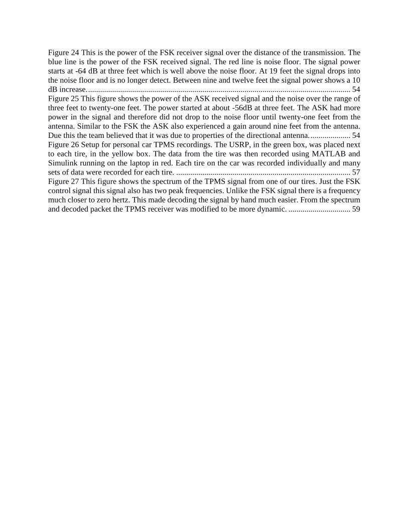
Figure 24 This is the power of the FSK receiver signal over the distance of the transmission. The

blue line is the power of the FSK received signal. The red line is noise floor. The signal power

starts at -64 dB at three feet which is well above the noise floor. At 19 feet the signal drops into

the noise floor and is no longer detect. Between nine and twelve feet the signal power shows a 10

dB increase. ................................................................................................................................... 54 Figure 25 This figure shows the power of the ASK received signal and the noise over the range of

three feet to twenty-one feet. The power started at about -56dB at three feet. The ASK had more

power in the signal and therefore did not drop to the noise floor until twenty-one feet from the

antenna. Similar to the FSK the ASK also experienced a gain around nine feet from the antenna.

Due this the team believed that it was due to properties of the directional antenna. .................... 54 Figure 26 Setup for personal car TPMS recordings. The USRP, in the green box, was placed next

to each tire, in the yellow box. The data from the tire was then recorded using MATLAB and

Simulink running on the laptop in red. Each tire on the car was recorded individually and many

sets of data were recorded for each tire. ....................................................................................... 57 Figure 27 This figure shows the spectrum of the TPMS signal from one of our tires. Just the FSK

control signal this signal also has two peak frequencies. Unlike the FSK signal there is a frequency

much closer to zero hertz. This made decoding the signal by hand much easier. From the spectrum

and decoded packet the TPMS receiver was modified to be more dynamic. ............................... 59

Executive Summary

Due to the ubiquity of tire pressure monitoring systems, or TPMS, since the passing of the

TREAD act, a concern has grown that these systems are vulnerable to wireless hackers. An article

in MIT's Technology Review details the very real possibility of this threat. The article released

in August of 2010 mentions a team that performed studies on the reception of information from

the TPMS [1]. Using equipment similar to those used in this study, the researchers in the article

were able to decipher the communication protocol of a TPMS module. There are several

implications to this technology; the first is that since the completion of the study radio technology

has improved substantially. The improvement in programmable radio technology has created less

expensive devices that can be purchased at an affordable cost. The price of these machines makes

them acceptable to everyone from hobbyists to those with malicious intent.

When a TPMS is hacked the hacker could possibly eavesdrop on the communication, give

false readings to a cars dashboard, track a vehicle's movements using the unique IDs of the pressure

sensors, and even cause a car's electronic control unit, or ECU, to fail; each of these resulting

outcomes would be an unacceptable security failure [2][3].

The purpose of this project is to test the feasibility of such a hacking. In order to do this

low cost readily available programmable radios were used to try and receive the TPMS signal. The

software used to manage the radios was MATLAB another readily available and relatively low

cost software. This report was meant not only to detail the results of the testing but to setup the

groundwork for future testing and implementation. Once a receiver can be developed that can pick

up the packets from the TPMS then further testing can be done in order to improve the security of

the TPMS to ECU communication.

The first experiment tested whether or not the universal software radio peripheral, or

USRP, would be capable of picking up the transmission of the TPMS modules. This was done by

having several controlled experiments in an isolated environment to remove any noise that could

disrupt the signal. Using two TPMS modules whose communication protocols were known the

USRP radio was used to try and identify their transmissions. Once the USRP proved capable of

receiving data from the TPMS in a controlled environment further testing was done to measure the

reliability of this communication at a distance.

The TPMS transmit signal is very weak as it only needs to travel a short distance to make

it to the ECU of the vehicle. If a third party receiver wanted to pick up this signal at a distance it

would require a focused antenna and an amplifier to increase the signal amplitude. The second

round of testing added these supplementary devices to the receiver in order to measure the distance

that the TPMS packets could be received. This test was important as the practicality of the hacking

threat becomes null if the signal can't be picked up from a distance. The same TPMS modules used

in the first experiment were also used in the second testing. This was to control for everything

other than the distance of the receiver from the TPMS. The success of this test prompted moving

on to a third experiment.

The third test was to try and receive the TPMS signal from a parked personal vehicle. This

experiment was conducted in order to test the decoding scheme on the receiver. A TPMS module

on a personal vehicle would have an unknown packet structure. In a real world application the

packet structure of the TPMS signal from a random vehicle would be unknown. This round of

testing was necessary to update the decoding scheme so it would be capable of receiving packets

from unknown TPMS modules. The successful reception of data from one a personal vehicle

prompted a fourth round of testing that would be conducted in a real world scenario.

The final round of testing which was to be roadside testing involved setting up the

directional antenna with power amplifier and USRP to try and measure packets from vehicles in

normal use. The roadside tests have not been completed and the feasibility of the threat remains

uncertain.

The overall goal for this project was to design a fully dynamic receiver for the TPMS

sensor. This was accomplish through the collection and analysis of data recorded by the tests

throughout the project. The receiver was starting point for future projects to continue on hacking

into a car’s CANBUS through TPMS sensors. This would first require building a transmitter

function to spoof the TPMS packet and research on how to hack into the CANBUS. Additionally

the directional antenna setup would need to be improved in order to collect packets from cars on

the road.

1 Introduction

The purpose of the TPMS is to monitor the air pressure in a car's tires. The TPMS is

primarily for safety as under and over inflated tires could cause accidents. An under-inflated tire

is one that does not fall between the acceptable tire pressure range on a car of 28 and 35 pounds

per square inch [5]. Incidents during the late 1990s included more than 100 automotive fatalities

due to under-inflated tires, causing the passing of the TREAD act [5]. The TREAD (Transportation

Recall Enhancement, Accountability, and Documentation) act, established two mandates. The first

mandate required tracking of, and response to, any possible danger signs from vehicles that would

require a recall or posed a safety risk. The second mandate required that all vehicles built in the

U.S. after 2007 must include a TPMS of some kind [5]. Today, the ubiquity of the TPMS

technology is taken for granted by the average consumer, creating a significant risk if the

communication between the TPMS and ECU is compromised. In order to test the security of the

TPMS, the goal of this project was to develop a receiver that could pick up TPMS packets on any

car in real time on the road.

1.1 Current State-of-the-Art

Current TPMS technology involves two methods for measuring and communicating the

tire pressure. The first is called a direct monitoring system [8]. This system includes attaching a

pressure sensor/transmitter to the vehicle's wheels. An in-vehicle receiver warns the driver if the

pressure in any tire falls below a predetermined level. These types of systems are typically more

accurate and expensive than their counterpart, the indirect monitoring system [8].

The indirect monitoring system uses the vehicles anti-lock braking system's wheel speed

sensors to compare the rotational speed of one tire versus the others. A small change in tire pressure

results in a change in the circumference in one of the tires. This change can be measured as a

change in speed. The indirect method is not the most reliable as it can lead to false alarms but it is

more cost effective (for the manufacturer) than the direct method.

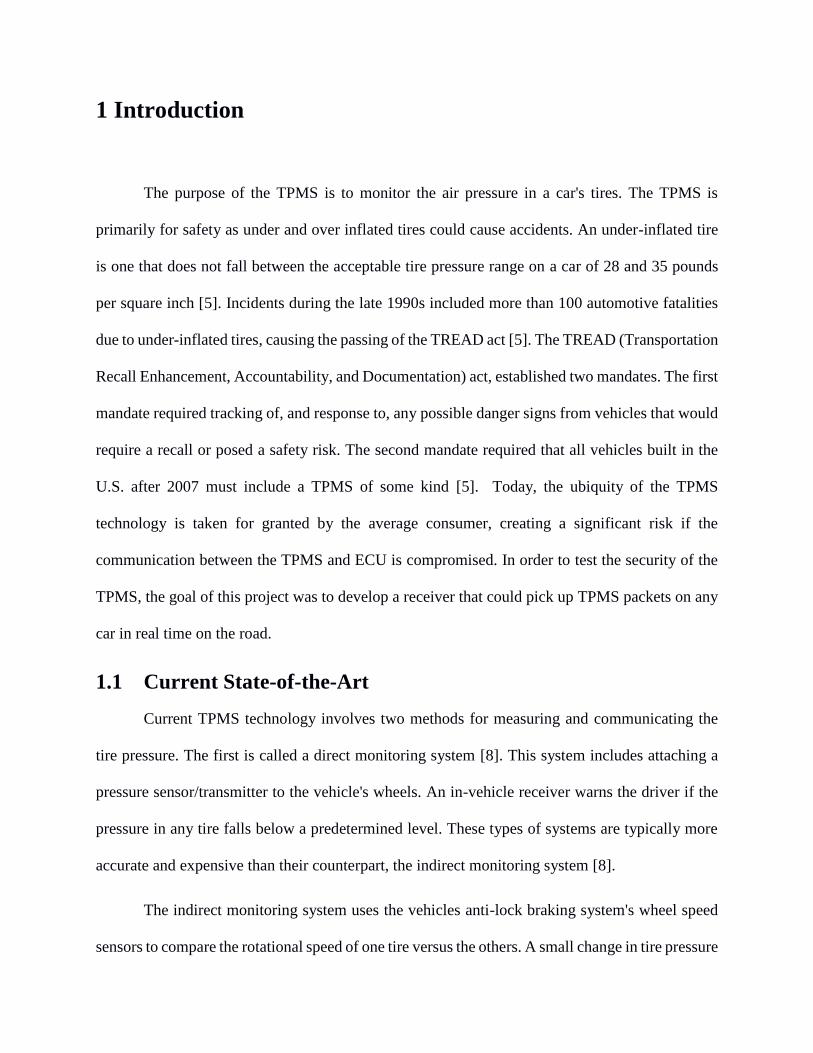
Figure 1 Above is a figure of the TI TPMS monitoring system. It is a direct monitoring system that uses a ceramic

capacitive sensor to measure tire pressure. This TPMS is connected to the tire valve and transmits to the ECU via a

RF Tx. [9]

The current state of TPMS technology makes the modules vulnerable to hacking.

According to the MIT article [1], researchers concluded that hackers could “hijack” the wireless

pressure sensors built into many cars' tires. The team of researchers successfully hijacked two

popular TPMS modules. By hacking into the module the research team could eavesdrop on

communication and, alter messages in-transit. The possibility of a hacking is a threat but there are

several hurdles that attackers have to jump over to succeed. One of these hurdles is that the tires

sensors communicate infrequently – about once every 60 – 90 seconds, making it difficult to

manipulate the system [1]. The way the research team was able to overcome this problem was by

shadowing the vehicle and using directional antennas to pick up the signals [1]. Another article

provides further evidence of the capability of tracking vehicles using TPMS [2].

Each TPMS sensor has a unique identification number. This can be read using an off-the-

shelf receiver [2]. What makes this technology dangerous is its ubiquity and the fact that the user

cannot turn off a TPMS sensor. Given the battery life on active sensors and the fact that passive

sensors do not require a battery, an attacker could keep surveillance on a vehicle for years [2].

1.2 Potential Issues with Testing

The major issues with the implementation of this project was the interfacing of the Ettus

N210 Software-Defined Radio (SDRU) with the available computers. All equipment necessary to

do testing was available, but the software to run the SDRU and measure the transmitted output of

the TPMS modules needed to be configured specifically for this experiment. The software used

was MATLAB and there were many interfacing problems that had to be overcome to do testing.

The next major issue was verifying the difference between random noise and actual data.

This was accomplished using signal processing techniques after reception of a signal from a

transmitting controller on the TPMS frequency.

1.3 Project Contributions

The majority of the equipment necessary to do testing was readily available at a flexible

price. The greatest expense was the downloading of a student version of MATLAB to run on a

personal computer. This version was purchased in order to do off-campus testing.

TPMS modules developed by TI were purchased for testing. The two modules that were

purchased used an FSK and ASK waveform for transmitting data. In order to power these modules

without connecting them to a battery an APEQ transmitter was used. The transmitter sent a signal

to the TPMS modules to activate them and have them send a signal that could be picked up by the

receiver.

A directional horn antenna and HPA were also used for this project. These two pieces of

equipment were borrowed from the available WPI laboratories.

1.4 Project Report Organization

This report is a thorough investigation into the possibilities of a security risk involving

TPMS modules. It explains the motivation of the project, the results of the testing and what those

results imply for the future of automotive security. In addition it details the possible issues with

implementation that someone wanting to repeat this project may face in the future. In the

Background section, the report details the knowledge required to have full understanding of the

results of this paper, including the types of sensors used on the TPMS modules, the communication

of the TPMS modules and the computer system, the information that is sent to the computer on the

car via the TPMS transmitter and detailed information on the SDRU and its application. The

Proposed Approach section describes the project from a systems level perspective. The proposed

approach section also details the course of the project and how each task was accomplished. The

Controlled Environment Section explains the signal waveform that can be received from the TPMS

transmitter. This section details the results of the analysis and the information gained from its

results. The results of the analysis are used to build a receiver that can pick up on the transmissions

from the TPMS. The Directional Antenna Distance Testing section details the results of adding a

directional antenna with a power amplifier to pick up on the signals being received from the TPMS.

The section goes over the procedure used for testing and the experiment control variable in order

to verify accurate results. The Personal Car Testing section outlines the procedure of using the

receiver to measure the TPMS packets from personal vehicles. This section lays out the

methodology of the testing and the subsequent results. The purpose of this section is to try and

decode the signal packets from an unknown TPMS module. The Roadside Testing section details

the future experimentation of the receiver’s capacity on the road. This section develops a process

in which future project groups can use the receiver in order to analyze packets from the TPMS

transmitter.

2 Background

This section of the report walks through all necessary information to understand the project.

A detailed overview of TPMS and the systems used in its construction are explained. This includes

information on the types of TPMS technology, the sensors used, and an overview of the

architecture. This section proceeds to explain the waveform types used in the TPMS modules used

for testing. This includes an explanation of both FSK and ASK waveforms. An overview of the

software defined receiver and its functionality is given. This includes a brief description of the

purpose of the SDRU and its capabilities. The final part of this section describes the directional

antenna and high power amplifier.

2.1 Tire Pressure Monitoring System

The tire pressure monitoring system (TPMS) is an electronic system designed to report

real-time tire-pressure information to the driver of the vehicle. TPMS was added to vehicles in

order to reduce traffic accidents occurring due to low pressure tires. “The installation of the system

(TPMS) is expected to contribute greatly to reducing traffic accidents….” [4]. The use of TPMS

has become mandatory for new vehicles beyond the United States. “The EU decided to make

TPMS mandatory for new vehicle type approvals by November 1, 2012 as well as for new vehicle

registrations by November 1, 2014...” [5]. With TPMS being the standard in modern vehicle tire

safety a new opportunity for businessmen everywhere has opened up. In 2012 there were 200

million TPMS sensors on the road. More than 35% of the sensors are now at least three years old.

That means an estimated 9 million sensors needed to be replaced in 2014 [6]. TPMS has also

presented significant risks. Beyond simple maintenance and false alarm concerns there is a

possibility that TPMS could be hacked into wirelessly [2]. One of the application of TPMS hacking

is tracking vehicles via the TPMS unique identifier. Each wheel of a vehicle equipped with TPMS

transmits a unique ID, which is easily readable using off-the-shelf receivers [3]. Given the

possibility of this threat an understanding of TPMS is necessary to calculate the probability and

nature of this threat.

There are generally two types of TPMS system direct and indirect. The direct system uses

a pressure transducer mounted inside the wheel to measure the pressure, and send that information

wirelessly to one more antennas on the body of the car. The types of pressure sensors are

piezoresistive sensor, capacitive sensors, and surface acoustic wave, or SAW, device. [9]. The

sensors take the pressure measurements and then send them to an antenna unit on the TPMS that

modulates them with a specific waveform. Two specific waveforms were used during the course

of testing one TPMS Amplitude Shift Keying, or ASK, module and a Frequency Shift Keying, or

FSK, module. The ASK and FSK modules were used as known variables to test the capabilities of

the receiver. These waveforms are products of the TPMS system. A TPMS system is composed of

multiple units and these units come together to form a waveform that is then sent out to the ECU.

2.1.1 Indirect TPMS system

The indirect TPMS method uses wheel speed sensors and the ECU which already exists in

the car to infer low tire pressure by looking for a wheel that is spinning faster than the others. This

technique works by comparing the speed of each wheel in normal driving mode, since a tire's

rolling radius depends on the air pressure inside. This method reduces implementation cost by

taking advantage of the anti-lock braking system, or ABS, of the vehicle. An image example of

the indirect approach to TPMS is displayed in Figure 2. A vehicle manufacturer that has been

using indirect TPMS in some of their models since 2013 is Honda. The Honda indirect TPMS

system uses the vehicle's ABS/VSA (Anti-lock Braking System/ Vehicle Stability Assist) wheel

speed sensors to calculate tire pressure [10]. This is a change in the status quo as indirect TPMS

wasn't used as frequently as direct TPMS due to its limitations.

Figure 2 This figure displays the use of an indirect TPMS system. As can be seen there are no added features to the

vehicle. All that is used are the wheel speed sensors in combination with the ABS system to measure differences in

wheel speed. The wheel that is rotating the fastest is considered to have less tire pressure. This is because as the tire

pressure decreases, the circumference of the wheel decreases along with it. A wheel with a small circumference will

rotate faster than those with a larger circumference in order to keep pace [9].

There are several problems associated with indirect TPMS that are not associated with

direct TPMS. These issues are listed below:

1. The system needs to be calibrated before it can sense different tire conditions. In

addition, changing a tire requires resetting the system to relearn the dynamic relationship

between each wheel.

2. An indirect TPMS at times has difficulty detecting low tire pressure.

3. Slip at the wheels disturbs the pressure-sensing algorithm.

4. Speed, acceleration, uneven tire wear and production tolerances affect rolling radius.

5. The system is unable to detect tire deflation of typically less than 30%

One example of an indirect tire monitoring system is the Tire Pressure Warning System

developed by Dunlop Tech GmBH. The Warnair developed by Dunlop is the indirect tire

monitoring system. Unlike direct systems it uses signals and measuring parameters already

available within the vehicle to measure tire pressure [12]. Corrosion is just one of the many issues

when dealing with direct TPMS sensors. Direct is much more accurate than indirect in its ability

to measure tire pressure but it requires maintenance. There are entire web pages dedicated to the

maintenance and repair of this type of TPMS sensor [7]

2.1.2 Direct TPMS

Direct TPMS utilizes sensors installed inside tires to measure and feedback the pressures

and temperatures directly. Wireless technologies for data transmission have to be used, because

the wheel is a rotating system which can't be connected by a wire. Direct TPMS uses RF

technology for transmitting sensor data to the vehicle. The most commonly used frequency for

transmitting tire information to the receiver is about 433 MHz In the U.S. a frequency of 315 MHz

is commonly used. The receiver for direct TPMS consists of an antenna, processor, memory and a

user interface. Figure 3 illustrates the additional equipment necessary to use a direct TPMS.

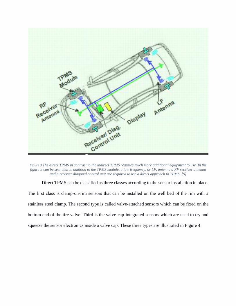
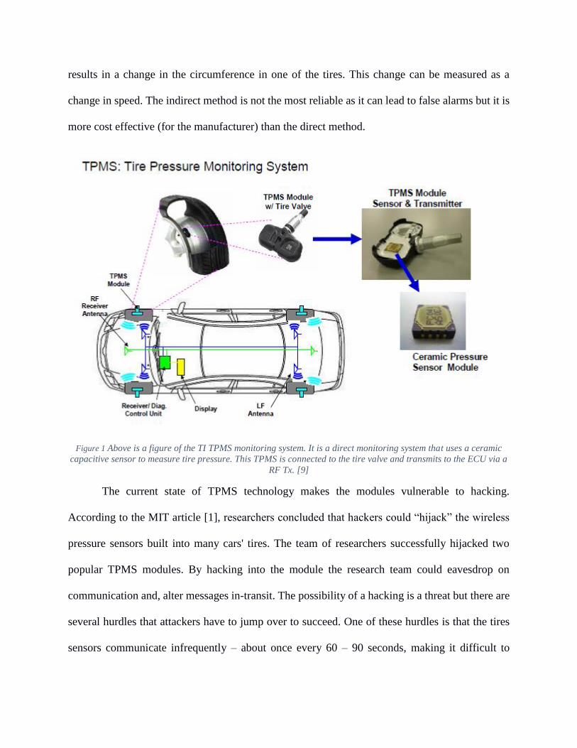
Figure 3 The direct TPMS in contrast to the indirect TPMS requires much more additional equipment to use. In the

figure it can be seen that in addition to the TPMS module, a low frequency, or LF, antenna a RF receiver antenna

and a receiver diagonal control unit are required to use a direct approach to TPMS. [9]

Direct TPMS can be classified as three classes according to the sensor installation in place.

The first class is clamp-on-rim sensors that can be installed on the well bed of the rim with a

stainless steel clamp. The second type is called valve-attached sensors which can be fixed on the

bottom end of the tire valve. Third is the valve-cap-integrated sensors which are used to try and

squeeze the sensor electronics inside a valve cap. These three types are illustrated in Figure 4

Figure 4 The first class of direct TPMS is illustrated in the picture to the far left. This is a clamp-on-rim TPMS

sensor. The second class is displayed in the middle and that is a valve-attached sensor. The third class is displayed

on the far right is the valve-cap integrated sensor [11].

There are two types of direct TPMS according to how the sensor is being powered. The

first is the active sensor, which is a sensor that contains a component for electric power. For an

active sensor the battery becomes the most problematic type component on the sensor, as it limits

the operating life time. The other type is the passive sensor. This sensor does not use battery power,

and instead receives power from other sources such as RF radiation from the ECU or a generator

near the sensors.

There are some problems with using direct TPMS sensors. As these sensors have a physical

presence on the tire, unlike indirect sensors, they usually do not last as long. One of the problems

with direct TPMS sensors that was discovered was that those with Metal Valve Caps tended to

corrode [7]. A solution to this problem was to add rubber valve caps that were not sensitive to

things such as moisture. Even with the maintenance issues that are common in direct TPMS this

system is the most commonly used.

The piezoresistive sensor causes a change in the electrical resistivity of a semiconductor or

metal when mechanical strain is applied. “The piezoresistive sensor has the advantages of simple

fabrication process and signal circuits, and moreover, the performance of this last type of sensor

is easily affected by circumstantial impurities” (Tian, 2009). Figure 5 is one design for a

piezoresistive sensor. The benefits to this type of sensor is that it is small in size, can be placed on

one chip and is cost effective.

Figure 5 A piezoresistive pressure sensor in the TPMS module works in the following way. There is a silicon

diaphragm that is sensitive to changes in pressure. A small change in pressure will cause the diaphragm to apply

more or less pressure on the piezoresistive element, thus causing a change in current through the circuit. This is

made clear in the figure via the circuit diagram. [14]

Piezoresistive pressure sensors are developed through the use of anisotropic chemical

etching and glass anodic bonding [17]. Etching is a common technique used in microfabrication

to chemically remove layers from the surface of a wafer during manufacturing [16]. Glass anodic

bonding is a bonding process that is used to seal glass to a silicon wafers without introducing an

intermediate layer [18]. These processes are used to develop the piezoresistive sensors. The

benefits of using these processes is that they create small affordable sensors. Piezoresistive sensors

have found other applications in vehicle manufacturing. Piezoresistive sensors are typically used

in three application areas: engine optimization, emission control, and safety enhancement [19].

The piezoresistive sensor is one of the most common sensors used in automotive manufacturing

as it is both space and cost efficient [5].

There is generally one of two types of capacitive sensors that is used in a TPMS sensor,

silicon microelectromechanical systems (MEMS) and ceramic [10]. MEMS is a technology that

manufactures very small devices. Capacitive pressure sensors of the MEMS variety have high

pressure sensitivity, low temperature sensitivity, good direct current (DC) response and low power

consumption. Their ability to handle changes in temperature make them capable outdoor sensors.

The Texas Instruments TPMS module used for testing employs a capacitive sensor [10]. Figure 6

illustrates the ceramic capacitive sensor being used in the TI TPMS module. An example of a

modern TPMS module that uses capacitive sensing is Freescale's MPXY8300. The MPXY8300 is

the first TPMS module to implement a pressure sensor, an 8-bit MCU, an RF transmitter and a 2-

axis (XY) accelerometer all in one package. The MPXY8300 is an example of how TPMS using

capacitive sensing technology has evolved to hold more devices in a small package [20].

Figure 6 This is the ceramic capacitive sensor that is used in the TI TPMS module for controlled experiments. There

are many benefits to using ceramic vs silicon capacitive sensors. They are relatively low cost, they have a simple

structure, they do not react strongly to chemical stress and they do not have great power dissipation losses. [10]

SAW sensors are a class of microelectromechanical systems which rely on the modulation

of surface acoustic waves to sense a physical phenomenon [26]. The way SAW systems measure

pressure is by using temperature compensation. Small changes in pressure relative to the other tires

can be measured and associated with a change in pressure [19] .One aspect of the SAW device that

differentiates itself from the other forms of sensing used in TPMS is that SAW does not require a

battery. The SAW sensor unlike other sensing types does not need a power supply unit or a wake-

up unit, and only requires an antenna for the transceiver unit [25]. The SAW device gets the energy

it requires from the radio signal it obtains from the antenna. The SAW sensor is of the passive type

unlike the capacitive and piezoresistive sensors that directly measure pressure via mechanical

changes [21]. An example of a SAW device is available in Figure 7 This SAW device was

developed by stackltd, a TPMS manufacturer [23].

Figure 7 Stackltd SAW TPMS. The device is batteryless and wireless. Used for motor-sport vehicles the device is

state of the art and offers a wide range of safety features for motor-sports. [23]

There are some academics and experts in the field of TPMS sensing that believe SAW is

the next generation of TPMS sensors [24]. A study conducted by Transense Technologies in the

UK concluded that a SAW device was able to measure pressure better than 0.4 psi. In addition to

this high sensor accuracy the system also demonstrated excellent sensor stability [22].

2.2 TPMS Communication ASK and FSK

TPMS modules have a Tx unit that sends sensor information on the tires to the electronics

control unit in the car. In the scope of this project and for testing purposes the two message

protocols to send sensor information was ASK (Amplitude Shift Keying) and FSK (Frequency

Shift Keying).

Amplitude shift keying in the context of digital communications is a modulation process

which imparts to a sinusoid two or more discrete amplitude levels. These would be the number of

levels adopted by the digital message. The waveform typically demonstrates sharp discontinuities

at the transition points.

Figure 8 In ASK the signal waveform is modulated to correspond with specific bit values. For instance in the figure it

can be seen that a waveform is produced when the bit value is high and the waveform is null when the bit value is

low. [27]

One of the disadvantages of ASK compared to FSK is the lack of constant envelope. This

makes processing more difficult. However it does make for easier demodulation with an envelope

factor.

FSK or frequency shift keyed transmitter has its frequency shifted by the message. There

can be more than two frequencies involved in FSK although in the figure only two are used.

Depending on the binary “key” of the message a different frequency is used to transmit that

message.

An FSK waveform has its frequency shifted by the message being transmitted. To use

Binary FSK as an example, the frequency of the waveform is shifted when the message is “on or

off”. In concept an FSK waveform can consist of two oscillators each on different frequencies. At

any point in time there can only be one oscillator connected to the output at any one time. This is

a brief description of how this waveform could be generated. The generation of this signal is

slightly more complicated than the generation.

There are multiple methods of demodulating FSK. There are asynchronous demodulation

which uses two bandpass filters that separates the signal into two parts. The output of each of these

band pass filters resembles an ASK waveform. These outputs are then passed through an envelope

detector and then a decision circuit. The decision circuit chooses the most likely of the envelope

outputs. Another commonly used method is a phase locked loop.

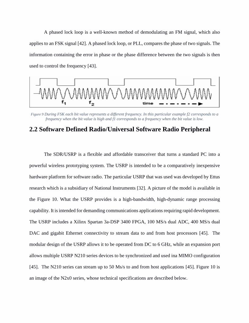
A phased lock loop is a well-known method of demodulating an FM signal, which also

applies to an FSK signal [42]. A phased lock loop, or PLL, compares the phase of two signals. The

information containing the error in phase or the phase difference between the two signals is then

used to control the frequency [43].

Figure 9 During FSK each bit value represents a different frequency. In this particular example f2 corresponds to a

frequency when the bit value is high and f1 corresponds to a frequency when the bit value is low.

2.2 Software Defined Radio/Universal Software Radio Peripheral

The SDR/USRP is a flexible and affordable transceiver that turns a standard PC into a

powerful wireless prototyping system. The USRP is intended to be a comparatively inexpensive

hardware platform for software radio. The particular USRP that was used was developed by Ettus

research which is a subsidiary of National Instruments [32]. A picture of the model is available in

the Figure 10. What the USRP provides is a high-bandwidth, high-dynamic range processing

capability. It is intended for demanding communications applications requiring rapid development.

The USRP includes a Xilinx Spartan 3a-DSP 3400 FPGA, 100 MS/s dual ADC, 400 MS/s dual

DAC and gigabit Ethernet connectivity to stream data to and from host processors [45]. The

modular design of the USRP allows it to be operated from DC to 6 GHz, while an expansion port

allows multiple USRP N210 series devices to be synchronized and used ina MIMO configuration

[45]. The N210 series can stream up to 50 Ms/s to and from host applications [45]. Figure 10 is

an image of the N2x0 series, whose technical specifications are described below.

This model is an example of the N2x0 series of USRPs offered by Ettus Research. The

advantages of the USRP N2x0 series are their technical specifications. In terms of hardware the

USRP N2x0 series have 1 transceiver card slot, external PPS reference input, external 10 MHz

reference input, MIMO cable shared reference, fixed 100 MHz clock rate, and an internal GPSDO

option. The FPGA on the N2x0 series is capable of 2 RX DDC chains in the FPGA, 1 TX DUC

chain in FPGA, Timed commands in FPGA, timed sampling in the FPGA, and 16-bit and 8-bit

sample modes [44].

Figure 10 This is the USRP used for the experiments conducted in this report. It is the USRP N210 Model developed

by Ettus research.[33]

The USRP can be used to receive messages from the TPMS system. Most USRPs connect

to a host computer through a high-speed link, which the computer software uses to control the

USRP hardware and transmit/receive data [34]. The USRP N210 which was used in the course of

experimentation is a high-performance USRP device that offers high dynamic range and

bandwidth [35]. The software used by the host computer to interface with the SDRU was

MATLAB [37]. There are specific libraries that can be used to interface with the SDR/USRP.

Within MATLAB, the modeling software SIMULINK is used to create block diagrams in order

transmit and receive data from the SDRU [36].

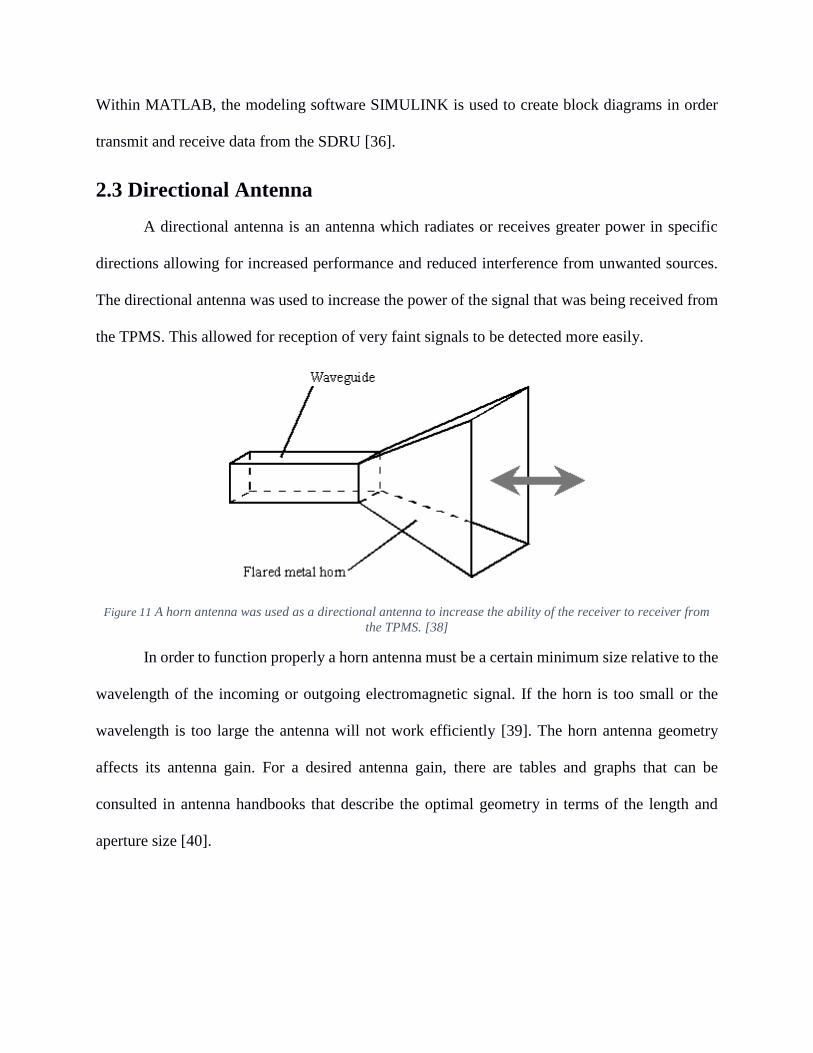
2.3 Directional Antenna

A directional antenna is an antenna which radiates or receives greater power in specific

directions allowing for increased performance and reduced interference from unwanted sources.

The directional antenna was used to increase the power of the signal that was being received from

the TPMS. This allowed for reception of very faint signals to be detected more easily.

Figure 11 A horn antenna was used as a directional antenna to increase the ability of the receiver to receiver from

the TPMS. [38]

In order to function properly a horn antenna must be a certain minimum size relative to the

wavelength of the incoming or outgoing electromagnetic signal. If the horn is too small or the

wavelength is too large the antenna will not work efficiently [39]. The horn antenna geometry

affects its antenna gain. For a desired antenna gain, there are tables and graphs that can be

consulted in antenna handbooks that describe the optimal geometry in terms of the length and

aperture size [40].

2.4 High Power Amplifier, or HPA

A high power amplifier is a device that takes an input signal and makes it stronger [29]. In

the case of this project the high power amplifier is used to amplify the weak signals of the TPMS

module before they go into the receiver. HPAs are used for multiple commercial purposes,

including increasing the signal for HDTV receivers [41].

2.5 Chapter Summary

This section outlines the background of the TPMS, USRP and directional antenna used in

this project. TPMS represents a system of elements used to monitor tire pressure. TPMS includes

the sensors, AFE, processing unit, and antenna. There are several types of methods that can be

used for TPMS and sensors. This gives some variety to the TPMS method that is used. The

SDR/USRP is the radio that is used to receive data from the TPMS system. The USRP can be

operated by using SIMULINK in MATLAB. A directional antenna was added to the USRP in

order to receive the transmission from the TPMS when the signal was too weak.

3 Proposed Approach

TPMS is a system that is vulnerable to external intentional attacks, as demonstrated by

other researchers [1]. Thus, it should be possible to test this threat by building a receiver that can

intercept these transmissions during normal vehicle operation. In order to test this theory, multiple

experiments were conducted in order to measure the actual TPMS data before taking it out into the

field.

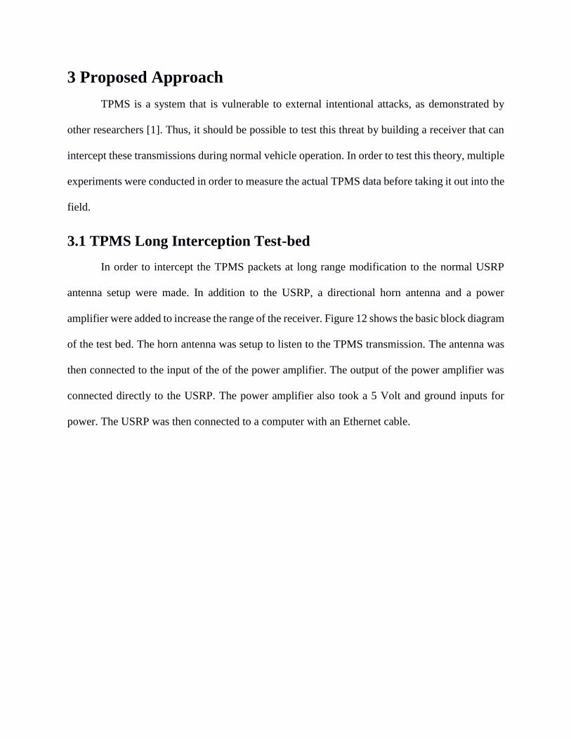
3.1 TPMS Long Interception Test-bed

In order to intercept the TPMS packets at long range modification to the normal USRP

antenna setup were made. In addition to the USRP, a directional horn antenna and a power

amplifier were added to increase the range of the receiver. Figure 12 shows the basic block diagram

of the test bed. The horn antenna was setup to listen to the TPMS transmission. The antenna was

then connected to the input of the of the power amplifier. The output of the power amplifier was

connected directly to the USRP. The power amplifier also took a 5 Volt and ground inputs for

power. The USRP was then connected to a computer with an Ethernet cable.

Figure 12 Long Range Interception Test Bed. In Red is the directional horn antenna which is connected to the input of the power

amplifier in green. The power amplifier also takes 5V and ground from the power supply in orange. The power amplifier sends

the amplified signal to the USRP in blue. The USRP modulates the signal down to the baseband and passes the data to MATLAB

and Simulink running on a computer through an Ethernet cable in purple. MATLAB and Simulink then perform the demodulation

and the decoding on the TPMS signal.

3.2 Testing Procedure

A system of tests was used to qualify the validity of the implementation of a receiver that

could pick up a TPMS signal during normal vehicle operations. The flow diagram in figure 13

describes the sequence of tests that were made.

Figure 13 Flow Diagram of the system of tests. From left to right, the 1st test done in a laboratory, the 2nd test to measure

maximum distance, 3rd test using a personal vehicle, and 4th test to test the practicality of this application.

These tests were pass or fail experiments. Each one dictated the continuation of the next

test. The first test was conducted in a laboratory in order to provide for maximum control. Two

DORMAN TPMS modules, part numbers 974-063 [43] and 974-026 [44], will be used, one using

ASK and the other using FSK for control. As these waveform modulations were known, it was

straightforward whether the USRP would pick up the signal. In order to do this, the ATEQ VT15

activator [42] was pointed at the TPMS modules while they were placed on top of the USRP. The

signal that was picked up from the USRP was later decoded to find the packet structure of the

TPMS module.

The second set of tests involved using a directional antenna and a power amplifier in order

to receive the weak signals from the TPMS. This set of tests will be used in order to measure the

TPMS from a distance. The results of this test will prove whether or not real world application

using these devices would feasible. The same TPMS modules used in the first test will be used in

this test. This is required to control for everything other than distance. This will prove whether or

not the antenna and power amplifier are viable options to receiving the signal from a TPMS at a

distance.

The third test involved trying to pick up a TPMS signal from a personal vehicle. To conduct

this test the receiver was taken out of the laboratory and placed next to the tire of the personal

vehicle. The ATEQ activator tool was pointed at the rim of one of the tires in order to activate the

TPMS. The USRP was then positioned in front of or on top of the tire of interest. Using MATLAB

the SDRU was run several times in order to collect a signal that could be later tested and decoded

to find the TPMS signal packet of the vehicle. This test is similar to the first experiment but no

longer controls for the TPMS communication waveform.

The final test will be roadside testing. Successful completion of this test will prove that the

threat of communication compromise between TPMS and ECU is not only real but practical.

3.4 Project Management

With the abundance of work that each team member had to go through during the period

of this project, project management was key to overall success. The team organized itself in order

to optimize each member’s expertise with the required task. Schedules were flexible as both of the

partner’s schedules were equally dynamic. The schedule for the project is located in the Gantt Char

in Table 1. Any components purchased for the project was done as a team. The testing and the

resulting analysis was split between the two members. The report was also split between both

partners in order to balance workloads. Occasionally third party volunteers aided in the completion

of the project when both partners were unavailable to perform testing.

Table 1 Gantt Chart for Project Time Management

3.5 Chapter Summary

The testing of the TPMS was done in incremental experiments. These experiments acted

as spring boards that gave confidence to the success of further experiments. For each round of

testing different variables were controlled in order to get closer to real life application. The

successful completion of this project involved the management of hectic schedules. The schedules

and software interfacing problems were the only limiting problems in the development of these

experiments.

4 Controlled Environment Testing

The overall goal for this project was to design a generic and dynamic receiver using

MATLAB and the USRP to decode all TPMS signals received from cars on the road. Before

looking at packets from car in motion, a couple of tests were first performed in order to give the

team a better understanding of the TPMS transmission. The first test was the controlled test where

two TPMS sensors (one ASK and one FSK) and a TPMS activator were purchased. These sensors

gave us a good starting point for decoding the TPMS sensor because the IDs were provided and it

was simpler to control the environment. The controlled test was completed so that the team could

build a basic receiver as well as provide insight into the TPMS transmission.

4.2 Controlled Testing Procedure

In order to perform the controlled testing, the two TPMS sensors and the ATEQ VT15

activator tool [42] were purchased. The two sensors, DORMAN TPMS sensor 974-063 [43] and

974-026 [44] were acquired in order to see transmissions from both the ASK and FSK. In order to

power up the TPMS sensors, an activation signal needs to be transmitted to the sensor. The ATEQ

activator transmits all known activation signals. To run controlled tests, each TPMS sensor was

tested separately by running the activator and recording the result of the TPMS on the USRP.

4.2.1 Initial testing

The initial testing was used to start designing the demodulator and to find the sensor’s ID

in the transmission. The demodulator would be used to the take the signal waveform and convert

it to a bit stream. Since the sensor’s ID is provided with on the TPMS sensor, finding the ID in the

packet stream is an easy way to validate the demodulator. For these tests, each of the TPMS sensors

were recorded separately right out of the box using the activator tool to start the transmission and

the USRP to record the transmission. The activator bombards the TPMS with all possible

activation signals for approximately one minute. Thus, the USRP was set up to record the entire

minute and the recorded data was analyzed offline.

Figure 14 shows the spectrum of signal from the ASK TPMS sensor. Since ASK transmits

at single frequency that varies in amplitude, there is only one peak in frequency. The plot below

shows that the frequency for this ASK transmission is at 43.78 KHz above the center frequency

and -50.986 dBm down.

Figure 14 The spectrum of signal from the ASK TPMS sensor. The plot below shows that there is a single frequency peak for the

ASK transmission in the red circle. The frequency is at 43.78 KHz from the center frequency and 50.986 dBm down. This is the

expected from an ASK wave because ASK transmits its data by varying the amplitude from one to zero at one frequency.

After viewing the spectrum of the signal, the team also viewed the time domain waveform

of the signal shown in Figure 15. For this signal, the difference is clear between the binary 1s and

0s. From this plot the packet was recorded first by hand and manually decoded.

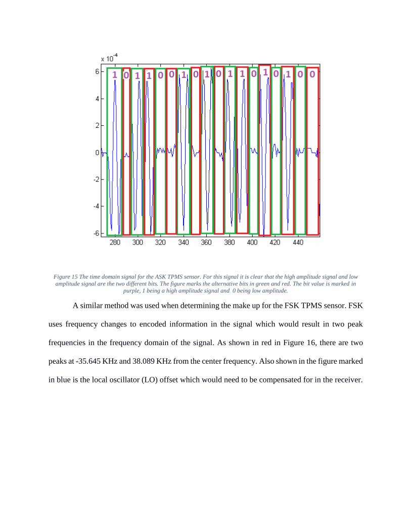
Figure 15 The time domain signal for the ASK TPMS sensor. For this signal it is clear that the high amplitude signal and low

amplitude signal are the two different bits. The figure marks the alternative bits in green and red. The bit value is marked in

purple, 1 being a high amplitude signal and 0 being low amplitude.

A similar method was used when determining the make up for the FSK TPMS sensor. FSK

uses frequency changes to encoded information in the signal which would result in two peak

frequencies in the frequency domain of the signal. As shown in red in Figure 16, there are two

peaks at -35.645 KHz and 38.089 KHz from the center frequency. Also shown in the figure marked

in blue is the local oscillator (LO) offset which would need to be compensated for in the receiver.

Figure 16 The figure shows the spectrum for the FSK received signal. As expected with an FSK encoded signal there are two

frequency peaks marked in red. The peaks occur at - 35.645 kHz on the right and 38.089 on the left. Also shown in the figure

marked in blue is the local oscillator (LO) offset which 1.302 kHz offset.

Just as the time domain of the signal was looked at for the ASK sensor, the time domain

was also viewed for the FSK sensor as well. Shown in Figure 17, the actual signal of the received

signal. Since the frequencies are close to the same in magnitude but on opposite sides of the

spectrum, the changes between bits would look like phase changes. Shown in red on the figure are

some of the phase changes between changes in bits. Upon looking at the signal it was quite difficult

to spot some of the changes and therefore the signal was manipulated to make the decoding easier.

Figure 17 The figure shows the time domain signal of the FSK. Since the frequencies were on opposite sides of the spectrum the

bit changes look like phase changes shown in red. Decoding this type of signal by hand if very tedious and there the signal was

shifted in order to make the simpler to decode by hand.

To make the decoding easier, the signal was shifted to the right in frequency to bring the

negative frequency to zero hertz of DC. Figure 18 shows that the negative frequency in red was

shift to DC and the positive frequency in green was shifted to 73.73 kHz. In the time domain this

would result in a high frequency signal and a DC signal for each bit.

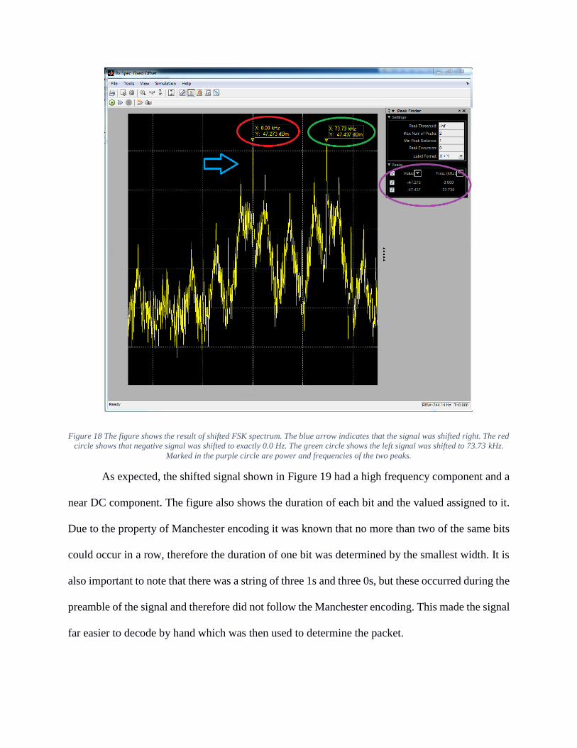
Figure 18 The figure shows the result of shifted FSK spectrum. The blue arrow indicates that the signal was shifted right. The red

circle shows that negative signal was shifted to exactly 0.0 Hz. The green circle shows the left signal was shifted to 73.73 kHz.

Marked in the purple circle are power and frequencies of the two peaks.

As expected, the shifted signal shown in Figure 19 had a high frequency component and a

near DC component. The figure also shows the duration of each bit and the valued assigned to it.

Due to the property of Manchester encoding it was known that no more than two of the same bits

could occur in a row, therefore the duration of one bit was determined by the smallest width. It is

also important to note that there was a string of three 1s and three 0s, but these occurred during the

preamble of the signal and therefore did not follow the Manchester encoding. This made the signal

far easier to decode by hand which was then used to determine the packet.

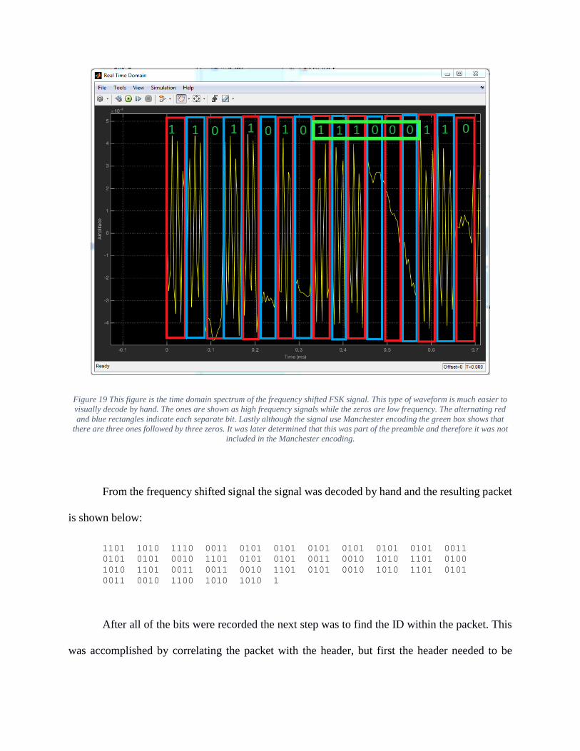
Figure 19 This figure is the time domain spectrum of the frequency shifted FSK signal. This type of waveform is much easier to

visually decode by hand. The ones are shown as high frequency signals while the zeros are low frequency. The alternating red

and blue rectangles indicate each separate bit. Lastly although the signal use Manchester encoding the green box shows that

there are three ones followed by three zeros. It was later determined that this was part of the preamble and therefore it was not

included in the Manchester encoding.

From the frequency shifted signal the signal was decoded by hand and the resulting packet

is shown below:

1101 1010 1110 0011 0101 0101 0101 0101 0101 0101 0011

0101 0101 0010 1101 0101 0101 0011 0010 1010 1101 0100

1010 1101 0011 0011 0010 1101 0101 0010 1010 1101 0101

0011 0010 1100 1010 1010 1

After all of the bits were recorded the next step was to find the ID within the packet. This

was accomplished by correlating the packet with the header, but first the header needed to be

converted from hexadecimal to binary, and then it needed to be Manchester encoded. A MATLAB

function find ID was created to take ID in hexadecimal as a string and the packet as an array. This

function converted the ID, performed the correlation and produced the maximum correlated value

and the corresponding index. Figure 20 shows the result of the MATLAB function and the plot of

the correlation of the signal. As expected, the maximum correlation was 32 since the ID was 64

bits with exactly thirty-two 1s and thirty-two 0s. Using the index of the correlation peak and the

length of the TPMS packet (length(TPMS_BITS)), the location of the ID (ID_loc) was solved for

using Equation 1. Using the location of the ID the packet was manually reformatted so that it could

then be decoded.

𝐼𝐷𝑙𝑜𝑐 = 𝑖𝑛𝑑𝑒𝑥 − 𝑙𝑒𝑛𝑔𝑡ℎ(𝑇𝑃𝑀𝑆𝐵𝐼𝑇𝑆) + 1 (Equation 1)

Figure 20 The figure is the result of the find_ID function. In yellow is the max value of the correlation and as expected for the 64

bit Manchester encoded packet the max is 32. The blue circle shows the index in the correlation where the max occurred which is

at position 208. In the green square is equation 1 that solves for the starting location of the ID in the packet from the index of the

max correlation value. The plot shows correlation of the packet and the ID, in red shows the max peak.

Using the index of the ID as a starting point the ID was located and marked. The following

bit stream below shows the original packet with the ID in bold:

1101 1010 1110 0011 0101 0101 0101 0101 0101 0101 0011

0101 0101 0010 1101 0101 0101 0011 0010 1010 1101 0100

1010 1101 0011 0011 0010 1101 0101 0010 1010 1101 0101

0011 0010 1100 1010 1010 1

After the ID was found the packet was reformatted and then decoded. The following bits

show the decoded packet with the ID in bold:

1000 0000 0000 0010 0000 1100 0000 1011 1100 0111 0010

1011 0000 1111 0000 1011 0111 11

The same method was followed when decoding the ASK received signal as well. From this

data a demodulator for the ASK and the FSK were made. These demodulators were verified by

comparing the outputted bits with the hand decoded bits. From the initial set of testing the signal

was manually decoded and the ID was found with the help of some MATLAB functions. Although

further testing needed to be completed in order to determine the meaning of the rest of the packet

using a controlled environment to change particular bits.

4.2.2 Controlled Testing

The controlled testing was used to determine the meaning of the rest of the TPMS packet.

In these tests the environment around the TPMS was changed in order to see the change in the bit

stream. Based on research it was known that the sensor would transmit the temperature and

pressure from its surroundings. Although varying the pressure was desired, time and resource

constraints made it so the team was unable to mount the sensor onto a tire. Fortunately, since the

pressure was zero and the team knew the location of the temperature bits, the pressure bits were

easily determined. Therefore, these tests were carried out by placing the TPMS sensor in glasses

of water with varying degrees and recording the results of the transmission.

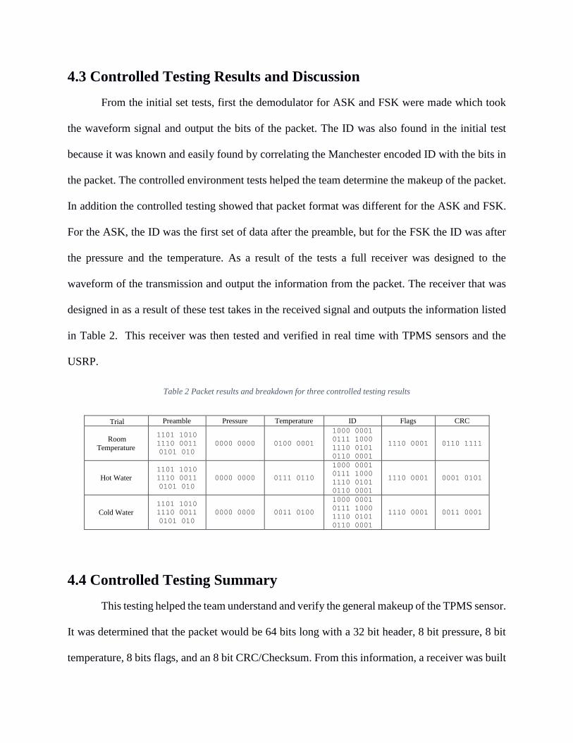
The results of the transmissions were recorded and then analyzed offline using the decoding

functions that were made after the previous tests. The results shown Table 2 the packets of three

test results (room temperature, hot water. and cold water) using the FSK TPMS sensor. From the

background research it was known that the data would come in groups of eight bits and the total

packet would be 64 bits. Based on this information and the changing bits, the team was able to

deduce that the bits marked in green were the temperature bits. Also as the temperature changed

the trailing bits changed as well and it was logically assumed to be the CRC or Checksum for the

packet. Although the pressure was not altered in these tests but kept constant at zero kPa, it was

determined that the eight bits before the temperature were the pressure and the five bits before that

were actually part of the preamble. Lastly the eight bits between the ID and the CRC/Checksum

were unknown, but from additional research they were assumed to be the battery life or flags.

From the background research it was known that cyclic redundancy check (CRC) or

checksum was used as validation checking. In order to determine whether it was a CRC or

checksum and to validate the packet later on, MATLAB functions were designed to help. The first

function simply solves for checksum and sees if it is valid. The other function that was made went

through every possible CRC pattern to determine if there was one or more possible combinations.

After running these functions on the FSK data, 100000111was a CRC pattern that was consistent

for all of the trials.

From the controlled testing the team was able to determine the make up for the TPMS

packet and determine the CRC pattern or checksum. From this information a full receiver and

decoder were created to take the waveform of the signal and output the information of the bits.

This function was first tested with recorded data and then modified to work with the USRP in real

time.

4.3 Controlled Testing Results and Discussion

From the initial set tests, first the demodulator for ASK and FSK were made which took

the waveform signal and output the bits of the packet. The ID was also found in the initial test

because it was known and easily found by correlating the Manchester encoded ID with the bits in

the packet. The controlled environment tests helped the team determine the makeup of the packet.

In addition the controlled testing showed that packet format was different for the ASK and FSK.

For the ASK, the ID was the first set of data after the preamble, but for the FSK the ID was after

the pressure and the temperature. As a result of the tests a full receiver was designed to the

waveform of the transmission and output the information from the packet. The receiver that was

designed in as a result of these test takes in the received signal and outputs the information listed

in Table 2. This receiver was then tested and verified in real time with TPMS sensors and the

USRP.

Table 2 Packet results and breakdown for three controlled testing results

4.4 Controlled Testing Summary

This testing helped the team understand and verify the general makeup of the TPMS sensor.

It was determined that the packet would be 64 bits long with a 32 bit header, 8 bit pressure, 8 bit

temperature, 8 bits flags, and an 8 bit CRC/Checksum. From this information, a receiver was built

Trial Preamble Pressure Temperature ID Flags CRC

Room

Temperature

1101 1010

1110 0011

0101 010 0000 0000 0100 0001

1000 0001

0111 1000

1110 0101

0110 0001 1110 0001 0110 1111

Hot Water 1101 1010

1110 0011

0101 010 0000 0000 0111 0110

1000 0001

0111 1000

1110 0101

0110 0001 1110 0001 0001 0101

Cold Water 1101 1010

1110 0011

0101 010 0000 0000 0011 0100

1000 0001

0111 1000

1110 0101

0110 0001

1110 0001 0011 0001

for each of the TPMS sensors and was able to decode signal in real time. Finally, it was noticed

how the TPMS sensor’s packets could vary even those sensors from the same manufacturer. From

the two sensors that were used, it was noted that the number of bits were different as well as the

packet format. Therefore the team understood the need and difficulty to make a fairly dynamic

receiver.

5 Directional Antenna Distance Testing

The major goal for this project was to produce a receiver that would be able to decode any

packet from any car in real time. Therefore USRP would have to be able to receive the TPMS

packets from cars on the road. Unfortunately the TPMS transmitter is very low power and the

USRP with the normal whip antenna would not be sufficient to receive the TPMS packet more

than a couple of feet away. Therefore a directional antenna and a power amplifier were added to

increase the range of the receiver. Before roadside testing was to be completed, the new setup was

first tested with the controlled TPMS sensors in order to gauge the distance of the receiver. This

test was completed the directional antenna, power amplifier and the two TPMS that were used in

the controlled testing.

5.2 Distance Testing Procedure

The distance testing was performed in order to find the optimal and maximum range for

the receiver with the directional antenna and power amplifier. This was also performed in order to

verify that the range would be sufficient for roadside recordings using a more controlled

environment. This test was performed using the FSK and ASK sensors that were used in the

controlled testing, as the receivers were already built. Therefore if the signal was of sufficient

power the receiver would be able to decode the packet. Both the FSK and ASK were tested to see

if there was any potential difference between the two that would cause one or the other to have a

greater range. Figures 17 and 18 show a close up of the power amplifier setup and a setup of the

whole system respectively.

Figure 21 This figure shows the setup of the Power Amplifier. The green arrow represents the data stream coming from the

antenna. The Blue arrow represents the signal going to the USRP. The red and purple box are the 5 volts and ground

respectively from the power supply.

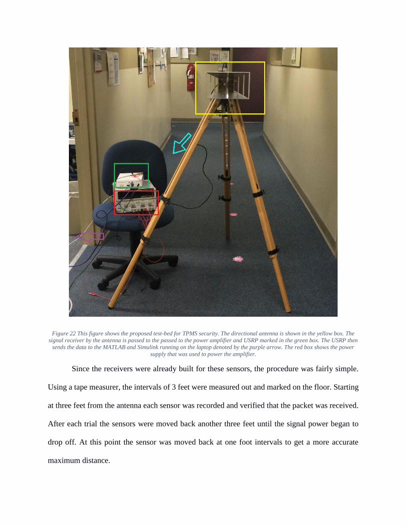
Figure 22 This figure shows the proposed test-bed for TPMS security. The directional antenna is shown in the yellow box. The

signal receiver by the antenna is passed to the passed to the power amplifier and USRP marked in the green box. The USRP then

sends the data to the MATLAB and Simulink running on the laptop denoted by the purple arrow. The red box shows the power

supply that was used to power the amplifier.

Since the receivers were already built for these sensors, the procedure was fairly simple.

Using a tape measurer, the intervals of 3 feet were measured out and marked on the floor. Starting

at three feet from the antenna each sensor was recorded and verified that the packet was received.

After each trial the sensors were moved back another three feet until the signal power began to

drop off. At this point the sensor was moved back at one foot intervals to get a more accurate

maximum distance.

5.3 Distance Testing Results

The test for both the ASK and FSK sensors showed that the sensor could be detected and

decoded up 18 feet away from the receiver. The plots in Figure 23 show the result of the FSK

transmission at 3 feet on the left and 18 feet on the right. The figure shows that the left signal

clearly stands out from the noise while the right signal is much closer to the noise floor. If the

sensor was any further away from the antenna the signal could not be differentiated from the noise.

Figure 23 Signal comparison for three feet signal and eight feet signal. Three foot signals in red clearly stands out from the noise

and easily decoded. The eighteen foot signals in green can still be seen but it is much closer to the noise floor and therefore more

affected by the noise.

The Figures 24 and 25 show the overall power levels of the received signals versus the

distance from the antenna. The first figure are the results from the FSK sensor and the second

results are from the ASK sensor. Both sensors showed a similar trend in the plots, generally

decaying as the distance increased. However it is important to note that both signals increased in

power around 10 to 12 feet which is most likely due to the gain of the antenna.

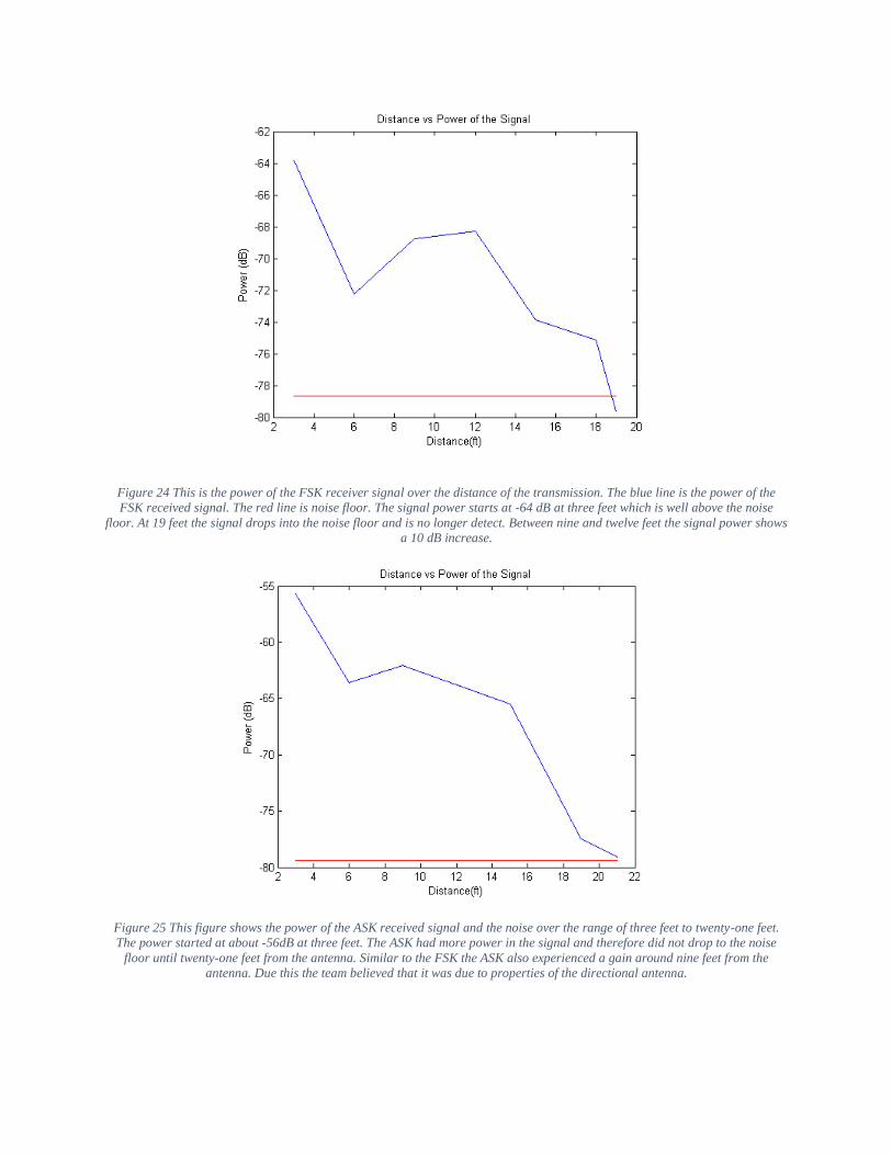
Figure 24 This is the power of the FSK receiver signal over the distance of the transmission. The blue line is the power of the

FSK received signal. The red line is noise floor. The signal power starts at -64 dB at three feet which is well above the noise

floor. At 19 feet the signal drops into the noise floor and is no longer detect. Between nine and twelve feet the signal power shows

a 10 dB increase.

Figure 25 This figure shows the power of the ASK received signal and the noise over the range of three feet to twenty-one feet.

The power started at about -56dB at three feet. The ASK had more power in the signal and therefore did not drop to the noise

floor until twenty-one feet from the antenna. Similar to the FSK the ASK also experienced a gain around nine feet from the

antenna. Due this the team believed that it was due to properties of the directional antenna.

5.4 Controlled Testing Summary

The distance testing was performed in order to determine the maximum and ideal range for

which the USRP, directional antenna, and power amplifier could accurately receive the TPMS

signal. This was accomplished by using the purchased FSK and ASK TPMS sensor and gradually

moving them away from the antenna. The results of this test showed that the system could

accurately record the TPMS packet up to 18 feet away. In addition this proved sufficient for

roadside because the antenna could be set up a safe distance from the road and still accurately

decoded the TPMS signal.

6 Real-World Evaluation

The overall final goal for this project was to design a generic and dynamic receiver for all

TPMS sensor variations. In order to do this the team would have had to listen to and record signals

from a variety of different cars. Before listening to random cars on the road the team wanted to

first test out their personal cars. This would provide the team with a more controlled environment

as some of the variables could be controlled in order to determine the packet. This would allow

more modifications to be made to the receiver before testing it on the road. In addition the

directional antenna would be used as well to test if the tires or car shielded the TPMS transmission,

reducing the range.

6.2 Personal Car Testing Procedure

The personal car testing was performed in a similar manner to controlled and distance

testing. The first set of tests were a done by controlling the environment as optimally as possible

in order to help determine the packet format. The data was collected by placing the USRP with the

normal whip antenna next to each tire one at a tire and recording the TPMS signal. In order to the

help determine the packet structure the environment needed to be controlled in order to change

specific bits at a time. The pressure bits were changed by adding and removing the pressure in the

tires and recording the results, and the temperature bits were changed by performing the readings

at different times of the day.

Figure 26 Setup for personal car TPMS recordings. The USRP, in the green box, was placed next to each tire, in the yellow box.

The data from the tire was then recorded using MATLAB and Simulink running on the laptop in red. Each tire on the car was

recorded individually and many sets of data were recorded for each tire.

The first test was performed in order to understand the packet and modify the receiver. The

second test involved using the modified receiver with the directional antenna. Data was recorded

from our personal cars in order to test the reliable distance of the TPMS transmitter when mounted

in a tire. This test was also performed in order to understand how and when all the TPMS sensors

in the car transmit together.

6.3 Personal Car Testing Results

After the tests were completed, the data were analyzed offline. Similar to the controlled

test, the packet was first decoded by hand and then a demodulator was created. In order to verify

that the demodulator worked it was compared to the packet that was manually decoded. In order

to determine the type of demodulator to use, the spectrum of the signal was first looked at in Figure

27. As seen in the figure there are two peak frequencies, indicating that the signal used FSK

modulation. From the new data the demodulator function was updated to make the receiver

dynamic.

Figure 27 This figure shows the spectrum of the TPMS signal from one of our tires. Just the FSK control signal this signal also

has two peak frequencies. Unlike the FSK signal there is a frequency much closer to zero hertz. This made decoding the signal by

hand much easier. From the spectrum and decoded packet the TPMS receiver was modified to be more dynamic.

During the demodulation the biggest problem that was encountered was that the waveform

signal and packets were of different lengths. Since the both the waveform lengths and the packet

lengths were different there was no clear correlation between the two sensors. Also since the packet

length is not known ahead of time for a random TPMS sensor the modulator was modified to make

it dynamic. The problem was solved by setting the samples per symbol much higher than the

expected samples per symbols and then using the MATLAB FSK demodulator function. The result

would cause an oversampling of bits being outputted by the demodulator. Then to down sample

the bits, the packet would first be traversed and the smallest number of consecutive bits was used

as the default size for a single bit. The function then traversed the packet again, down sampling

the down to the normal bit stream based upon the number of consecutive bits. Based upon the

results from our cars and the controlled sensors, this method worked well without having to

manually tune variables. In addition, an interpolation was added to provide additional accuracy.

After the signal was demodulated, the packet format would be determined by observing

the bits changes between trials and different tires. From the trials the Table 3 shows the format of

the packet with example data that was recorded. From our cars’ packets and the controlled sensor

packets, the packets clearly have different formats. From this information it can be assumed that

other cars packets will differ slightly as well. This will lead to difficulty in determining packet

structure in real time. To overcome not knowing the packet structure a MATLAB script was

created that started with that looked at all possible sequential 128 bits. The function performed

Manchester decoding and the attempted to brute force CRC. Since the CRC is 9 bits long then

there is a 1 in 512 chance that there is a valid CRC pattern. Therefore it was assumed that if a CRC

pattern was found then that must be the packet.

Table 3 Packet Structure for Personal Car TPMS Sensor and Example Data.

6.4 Personal Car Testing Summary

The test and recordings on the team’s personal cars were implemented in order to provide

another TPMS sensor to look at in a controlled environment before listening to uncontrolled cars

on the road. The directional antenna was also tested in order to gather more accurate distance

testing with regards to a TPMS sensor being mounted in a tire. From the data that was gathered in

Trial Preamble ID Temperature (F) Pressure (kPa) Flags CRC

Packet in Binary 1110 0000 0

1000 1000

0111 1100

0110 1001

1111 1001

0101 1010 1111 0000 1111 1000 0101 1100

Packet Values N/A 887C69F9 90 240 F8 5C

this experiment, four TPMS transmissions and packets were collected and analyzed. This new data

allowed the team to modify the receiver to be more dynamic by modifying the demodulator and

the packet decoding. After completing the modifications the biggest concern for making the

receiver dynamic is the unknown packet format. Lastly when performing this test it was noted that

the TPMS sensors were still able to transmit when the car was off and without activation. After

additional research it was found that some cars and sensors allowed for the sensor to always

transmit periodically if there is a receiver listening.

6.5 Roadside Testing

The final test for the project was to observe and record data TPMS packets from vehicles

traveling on the road. The recorded data would then be used with the current model of the receiver.

After analyzing the results, the receiver would be modified further if any changes were needed to

decode the TPMS packets. Lastly the modified receiver would be run in real time to prove that it

could decode TPMS packets from cars on the road.

For the roadside testing the directional antenna, power amplifier, and URSP were used.

Using the same configuration for the distance testing these were all set up on the edge of the side

walk next to Salisbury St. in Worcester, MA. The USRP was set up to run and record for

approximately two minutes at a time. Then the results would then be analyzed offline and used to

improve the TPMS receiver. After the TPMS receiver was modified it would be used to decode

TPMS in real time from cars traveling on the road.

After analyzing the data from the roadside testing there were no signs that any TPMS signal

was captured by the USRP. The team was planning to improve the configuration and retry the

roadside recordings. Due to timing constraints the team was unable to improve the tests nor was

the receiver tested in real time with cars traveling on the road.

The roadside recordings were gathered in order to test and improve the receiver. The

receiver was to then be tested by receiving and decoding TPMS from vehicles on the road in real

time. Unfortunately after the initial set of recordings there was no evidence of any TPMS signal

recorded by the USRP. Although the team wanted to improve the setup and run the roadside test

again, the team ran out of time to redo the test. Therefore the TPMS was unable to be tested in real

time with data from cars driving on the road.

7 Conclusion

The purpose of this project was to produce a receiver that could pick up messages from a

TPMS when a vehicle is in normal operation. In the process of making this receiver, several tests

were done in order to make incremental progress. The first of these tests, which involved a

controlled laboratory experiment, was successful. The team was able design a receiver to take an

ASK and FSK TPMS module and decode the individual packets. This project supports the idea

that snooping TPMS packets in real time in a real world situation would be possible, albeit difficult.

The difficulty of the task was the second conclusion drawn from the first round of testing. It was

discovered that message packets could vary even from TPMS devices from the same manufacturer,

thus the decoding scheme would be another hurdle to the successful design of a receiver.

The second round of testing involved the use of an antenna with power amplifier to improve

the ability of the receiver to receive at a distance. Within the second round of testing the team

wanted to draw a conclusion on what the limiting operating distance for the receiver to pick up a

signal of the TPMS would be. The receiver was aided by a directional antenna and a power

amplifier. The results of this analysis showed that the receiver could pick up TPMS signals up to

18 feet away, allowing the team to conclude that the receiver could be set up a safe distance from

roadside traffic and still be able to pick up a signal. Further testing using a personal vehicle can be

continued, not just utilizing an off-the-shelve TPMS module.

The third round of testing was done on the teams’ personal vehicles. The purpose was to

gather more TPMS data in a semi-controlled environment before moving onto roadside testing.

The conclusion drawn from this test was that the team would be dealing with uncertain roadside

packet structures. This unknown would make decoding more difficult as it requires changing the

decoding scheme for each packet structure. Research into an alternative solution has not yet been

conducted and could be possible.

8 Recommendations

The first recommendation would be to have all software and interfacing to the USRP done

as early as possible. Interfacing problems caused the most issues throughout the project and

delayed testing. Other recommendations include changing the nature of the experiment. The first

few rounds of testing proved that decoding the TPMS packets was possible. Road side testing was

not met with the same success. Continuing road side tests to find favorable conditions for its

success could be a future direction of the project. Beyond just the scope of this project a future

team could take the concept of wireless hacking further.

The team has a set proposed steps for continuing the TPMS car hacking. The first step

would be to learn of to jam the TPMS sensor on a car preventing the receiver from picking up any

data. This would cause the TPMS light on the dashboard to turn on. Next a transmitter would have

to be implemented in order to spoof the TPMS. This would be tested by changing TPMS

parameters until the light turns on. The last step before trying to hack the car through the TPMS

sensor is to research the CANBUS and the TPMS receiver in the car and develop a method for

hacking the car. This may require building a smaller test bed with just and CANBUS or receiver

in order to assist in the design. Finally implement the plan for hacking and test on a real car.

There are many electronic systems that use wireless technology on a vehicle. Everything

from wireless keys used to unlock the doors to radios can be wirelessly hacked. An article in the

technology magazine WIRED illustrates the potential threat of the wireless hacking of car keys. A

young hacker developed a system where the signal from wireless keys could be hacked via a small

radio device (Kamkar, 2015). This example is just another possibility of the future direction this

project can take.

9 Appendix

9.1 ASK_demodulator function

function [ packet ] = ASK_demodulator( rx ) %ASK_demodulator % Function performs ASK demodulation of the TPMS packet

%% Variable setup interp_val = 2; rx_interp = interp(rx, interp_val); lenRx = length(rx_interp); rx_rect = abs(rx_interp); threshold = max(rx_rect/2);

%figure %plot(1:lenRx, rx_rect)

%% Demodulation rx_square = zeros(1, lenRx); for x = 1:lenRx if rx_rect(x) > threshold rx_square(x) = 1; end end

%figure %plot(1:lenRx, rx_square); %% Down sampling packet = down_sample(rx_square);

end

9.2 CRC_pattern Function

function [ good_patterns ] = CRC_pattern( packet, p ) %CRC_pattern % this function takes in the packet and the length of the pattern and % solves for a CRC pattern using brute force

%% init vars dec_nums = 0:2^p-1; pattern_str = dec2bin(dec_nums); pattern = zeros(2^p, p); %% initializing the patterns array that will be checked for x = 1:2^p for y = 1:length(pattern_str(x,:)) pattern(x,y)= str2double(pattern_str(x,y)); end

end

n = length(packet); k = n - p + 1;

pattern(2^(p-1)+1,:);

good_patterns = zeros(1, p); good = 1; %% cycles through all potential patterns

for y = 2^(p-1)+1:2^p y; x = 1; div = packet(1:p); a = 0;

while div(1) == 0 && x+a < k div(1:end-1) = div(2:end); div(end) = packet(x+a+p); a = a + 1; end

x = a + x;

while x < k div = xor(div, pattern(y,:)); a = 0; while div(1) == 0 && x+a < k div(1:end-1) = div(2:end); div(end) = packet(x+a+p); a = a + 1; end x = a + x;

end % If the pattern works put it in the good patterns array

if sum (div == zeros(1,p)) == p || sum(div == pattern(y,:)) == p good_patterns(good, :) = pattern(y,:); good = good + 1; end end

end

9.3 decode_packet Function

function [ ] = decode_packet( packet ) %UNTITLED3 Summary of this function goes here % Detailed explanation goes here

packet_len = length(packet);

for p = 1:packet_len-128 decoded = man_decode(packet(p:p+127)); if decoded ~= -1 patt = CRC_pattern(decoded, 9); if sum(patt(1,:)) ~= 0 'non' decoded patt end end

decoded = man_decode(invert(packet(p:p+127))); if decoded ~= -1 patt = CRC_pattern(decoded, 9); if sum(patt(1,:)) ~= 0 'inv' decoded patt end end

end %[m,ind] = find_ID('77839606', packet) %[m,ind] = find_ID('887C69F9', packet) %[m,ind] = find_ID('8178E561', packet) %[m,ind] = find_ID('1C07902E', packet)

%[m,ind] = find_ID('DBDACB03', packet) %[m,ind] = find_ID('242534FC', packet)

%{ preamble_bits = packet(1:ind-1); length(preamble_bits); packet = packet(ind:end); decoded_packet = zeros(1, length(packet)/2);

for x = 1:2:length(packet) if packet(x) == 1 decoded_packet((x+1)/2) = 0; else decoded_packet((x+1)/2) = 1; end end

%packet_num = sum(decoded_packet .* 2 .^ (length(decoded_packet)-1:-1:0)) pressure_bits = decoded_packet(1:8); temp_bits = decoded_packet(9:16); ID_bits = decoded_packet(17:48); flags = decoded_packet(49:56); crc = decoded_packet(57:end);

count = 7:-1:0;

preamble = num2str(preamble_bits) temp = sum(temp_bits .* 2.^count) pressure = sum(pressure_bits .* 2.^count) ID = dec2hex(sum(ID_bits .* 2 .^ (31:-1:0))) %}

end

9.4 demodulator Function

function [ packet] = demodulator( rx, Fs ) %demodulator % Takes in the packet and the sample rate %This function determines if it uses ASK or FSK and then demodulates the %signal and passes the demodulated packet out

%perform the FFT and get magnitude freq = abs(fft(rx));

%figure %plot(1:length(freq), freq)

%range to prevent side bins from influencing results range = 10; [max1,ind1] = max(freq); %Determines the two max bins that are not closely adjacent if ind1 - range > 0 && ind1 + range <= length(freq) freq(ind1-range:ind1+range) = 0; elseif ind1 - range < 0 freq(1:ind1+range) = 0; freq(length(freq)+ind1-range:length(freq)) = 0; else freq(ind1-range:length(freq)) = 0; freq(1:(ind1+range)-length(freq)) = 0; end [max2, ind2] = max(freq);

%determines if the second frequency is large enough to be FSK if max2 > max1/2 [packet] = FSK_demodulator(rx,Fs); else [packet] = ASK_demodulator(rx,Fs); end end

9.5 down_sample Function

function [ down ] = down_sample( packet ) %down_sample % This function takes in a packet with excess bits from demodulation. and % downsamples based on the small number of consequtive bits

%% Starts a litte in because sometimes the first bits are compromised ind = 50; val = packet(ind); lenPacket = length(packet); %% finding the start of the next change so it does not throw off count while packet(ind) == val && ind < lenPacket ind = ind + 1; end

%% Calculates the min number of consequtive bits and is the default single

bit min_count = lenPacket; while ind < lenPacket-20

val = packet(ind); count = 0; while packet(ind) == val && ind < lenPacket count = count + 1; ind = ind + 1; end

if count < min_count min_count = count; end

end

%% performs the down sampling based on the min count above down = 0; down_ind = 1; ind = 1; while ind < lenPacket

val = packet(ind); count = 0; while packet(ind) == val && ind < lenPacket count = count + 1; ind = ind + 1; end

count = floor((count)/min_count); if count == 0 count = 1; end

a = 1; while a <= count down(down_ind) = val; down_ind = down_ind + 1; a = a+1; end

end

end

9.6 find_ID Function

function [ m, ind ] = find_ID( ID, signal ) %find_ID %This function takes the ID in Hex and the packet and solves for the %location of the ID within the packet using corr % The function outputs the max value and its index

%% Convert the ID to bin and then encode it ID_binary = Hex_to_Bin(ID); encoded_ID = man_encode0to0(ID_binary); %% perform corr and take the max val and index acor = xcorr(signal, encoded_ID); %figure %plot(1:length(acor), acor) %xlabel('Index') %ylabel('Correlation') %title('Correlation of Encoded ID and Encoded TPMS Packet') [m, ind] = max(acor);

end

9.7 FSK_demodulator Function

function [ packet] = FSK_demodulator( rx, Fs ) %FSK_demodulator %This function performs FSK demodulation on the signal and outputs the %packet %% variable intialization lenRx = length(rx); t = (1:lenRx)/Fs; interp_val = 20; bits_per_packet = 750; samp_per_sym = floor(interp_val * lenRx / bits_per_packet); down_samp = interp_val * lenRx - bits_per_packet * samp_per_sym; interval = floor(interp_val * lenRx / down_samp);

%% Adjusting the offset frequency

freq = max_frequencies(rx, Fs,2); offset = -(freq(1) + freq(2))/2; mod_sig = exp(j*2*pi*t*offset); rx = rx .* mod_sig;

%% Calculating the freq separation

freq = max_frequencies(rx, Fs, 2); freq_sep = abs(freq(1)) + abs(freq(2));

%% downsamples so there is an symbols per bits divides evenly down_samp_sig = zeros(1, bits_per_packet * samp_per_sym); rx_interp = interp(rx, interp_val);

for y = 1:down_samp down_samp_sig((y-1) * (interval-1) + 1:y * (interval - 1)) =

rx_interp((y-1) * interval + 1:y * interval - 1); end

%% Demodulates packet over_packet = invert(fskdemod(down_samp_sig,2,freq_sep,samp_per_sym,

Fs*interp_val)); %% Because more bits were output than needed a downsample is used packet = down_sample(over_packet);

%figure %plot(1:lenRx, abs(fft(rx)))

end

9.8 Hex_to_Bin Function

function [ bin ] = Hex_to_Bin( ID ) %Hex_to_Bin % this function takes in the ID in a hex string and converts it to a % binary array

binStr = dec2bin(hex2dec(strcat('A', ID))); bin = zeros(1, length(binStr));

for x = 1:length(bin) bin(x)= str2double(binStr(x)); end bin = bin(5:end); end

9.9 invert Function

function [ out ] = invert( in ) %invert % this function takes in a binary packet of ones and zeros and inverts each % bit out = in; for x = 1:length(in) out(x) = xor(1, out(x)); end end

9.10 man_decode Function

function [ decoded ] = man_decode( encoded ) %man_decode %This function takes in a manchester encoded signal and decodes it

decoded = zeros(1, length(encoded)/2); %takes every other value starting at 1 for x = 1:2:length(encoded) %making sure two succesive bits are not the same if encoded(x) ~= encoded(x+1) decoded((x+1)/2) = encoded(x); else decoded = -1; break; end end end

9.11 man_encode Function

function [ encoded_signal ] = man_encode( signal ) %man_encode % this function takes in a packet and manchester encodes it

%encoded signal is twice the length encoded_signal = zeros(1, 2*length(signal));

for x = 1:2:length(encoded_signal)

if signal((x+1)/2) == 1 encoded_signal(x) = 1; else encoded_signal(x) = 0; end encoded_signal(x+1) = xor(encoded_signal(x), 1);

end end

9.12 max_frequencies Function

function [ index ] = max_frequencies( rx, Fs, num_freqs ) %max_frequencies %This function takes the rx signal, sample rate and the number of maxs to %record %this function then outputs the frequency of the peaks

%% Init vars lenFFT = length(rx); freq_scale = (Fs /2) / (lenFFT / 2); freq = abs(fft(rx)); range = 10; index(1:num_freqs) = 0;

%% Picks the max for each freq but makes sure that adjacent values dont

interfere for a = 1:num_freqs [m,index(a)] = max(freq); freq(index(a)) = 0;

if index(a) - range > 0 && index(a) + range <= length(freq) freq(index(a)-range:index(a)+range) = 0; elseif index(a) - range < 0 freq(1:index(a)+range) = 0; freq(length(freq)+index(a)-range:length(freq)) = 0; else freq(index(a)-range:length(freq)) = 0; freq(1:(index(a)+range)-length(freq)) = 0; end

end %% Calcs the frequency of the peak for a = 1:num_freqs if index(a) > lenFFT/2 index(a) = (index(a) - lenFFT) * freq_scale; else index(a) = index(a) * freq_scale; end end

end

9.13 reformat Function

function [ array ] = reformat( vector, rows ) %Takes in a single demension array and formats it to multidemsional based %on the number of rows given

columns = floor(length(vector)/rows);

array = zeros(columns, rows);

for ind = 1:columns

array(ind,:) = vector((ind-1)*rows + 1:ind*rows);

end

end

9.14 TPMS_concat Function

function [ out, samples ] = TPMS_concat( in ) % This function takes in the input signal in the form of a multidemensional % array and concatenates them into a single demension

[x, y] = size(in);

out = zeros(1, x*y); samples = 1:x*y;

for a = 0:x-1

out(a*y+1:(a+1)*y) = in(a+1,:);

end end

9.15 TPMS_decode_by_ID_first function

function [ preamble, ID, pressure, temp, flags, crc, packet] =

TPMS_decode_by_ID_first( ID, TPMS_bits ) %this function assumes that the ID comes before the packet information % this function takes the ID as a Hax string and the packet

%finds the start of the packet [m, ind] = find_ID(ID, TPMS_bits) ind = ind - length(TPMS_bits) + 1; %takes the preamble preamble_bits = TPMS_bits(1:ind-1); %decodes the rest of the packet packet = man_decode(TPMS_bits(ind:ind+127));

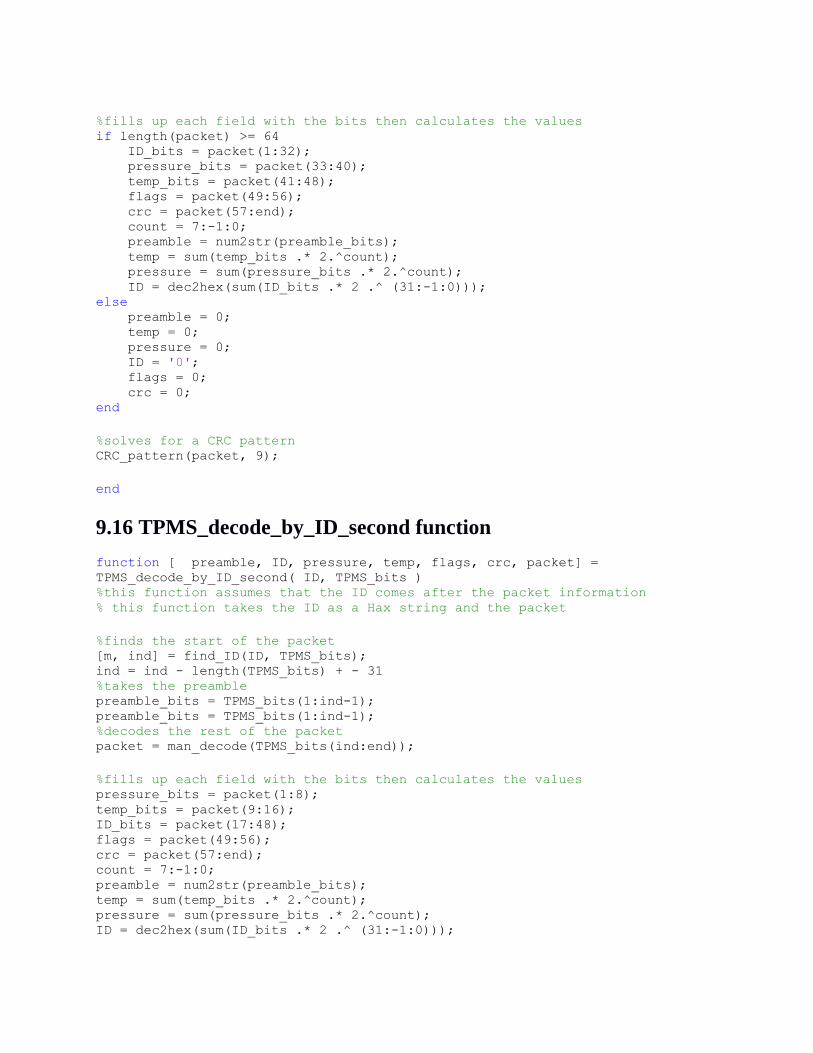
%fills up each field with the bits then calculates the values if length(packet) >= 64 ID_bits = packet(1:32); pressure_bits = packet(33:40); temp_bits = packet(41:48); flags = packet(49:56); crc = packet(57:end); count = 7:-1:0; preamble = num2str(preamble_bits); temp = sum(temp_bits .* 2.^count); pressure = sum(pressure_bits .* 2.^count); ID = dec2hex(sum(ID_bits .* 2 .^ (31:-1:0))); else preamble = 0; temp = 0; pressure = 0; ID = '0'; flags = 0; crc = 0; end

%solves for a CRC pattern CRC_pattern(packet, 9);

end

9.16 TPMS_decode_by_ID_second function

function [ preamble, ID, pressure, temp, flags, crc, packet] =

TPMS_decode_by_ID_second( ID, TPMS_bits ) %this function assumes that the ID comes after the packet information % this function takes the ID as a Hax string and the packet

%finds the start of the packet [m, ind] = find_ID(ID, TPMS_bits); ind = ind - length(TPMS_bits) + - 31 %takes the preamble preamble_bits = TPMS_bits(1:ind-1); preamble_bits = TPMS_bits(1:ind-1); %decodes the rest of the packet packet = man_decode(TPMS_bits(ind:end));

%fills up each field with the bits then calculates the values pressure_bits = packet(1:8); temp_bits = packet(9:16); ID_bits = packet(17:48); flags = packet(49:56); crc = packet(57:end); count = 7:-1:0; preamble = num2str(preamble_bits); temp = sum(temp_bits .* 2.^count); pressure = sum(pressure_bits .* 2.^count); ID = dec2hex(sum(ID_bits .* 2 .^ (31:-1:0)));

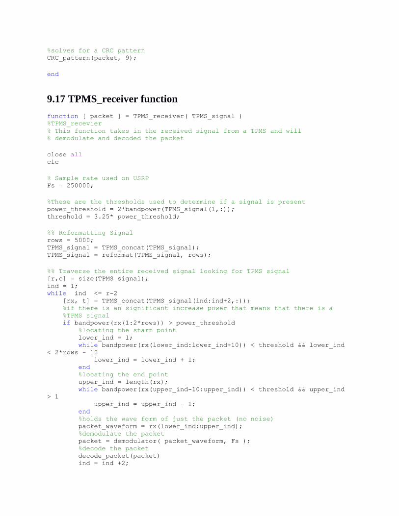
%solves for a CRC pattern CRC_pattern(packet, 9);

end

9.17 TPMS_receiver function

function [ packet ] = TPMS_receiver( TPMS_signal ) %TPMS_recevier % This function takes in the received signal from a TPMS and will % demodulate and decoded the packet

close all clc

% Sample rate used on USRP Fs = 250000;

%These are the thresholds used to determine if a signal is present power_threshold = 2*bandpower(TPMS_signal(1,:)); threshold = 3.25* power_threshold;

%% Reformatting Signal rows = 5000; TPMS_signal = TPMS_concat(TPMS_signal); TPMS_signal = reformat(TPMS_signal, rows);

%% Traverse the entire received signal looking for TPMS signal [r,c] = size(TPMS_signal); ind = 1; while ind <= r-2 [rx, t] = TPMS_concat(TPMS_signal(ind:ind+2,:)); %if there is an significant increase power that means that there is a %TPMS signal if bandpower(rx(1:2*rows)) > power_threshold %locating the start point lower_ind = 1; while bandpower(rx(lower_ind:lower_ind+10)) < threshold && lower_ind

< 2*rows - 10 lower_ind = lower_ind + 1; end %locating the end point upper_ind = length(rx); while bandpower(rx(upper_ind-10:upper_ind)) < threshold && upper_ind

> 1 upper_ind = upper_ind - 1; end %holds the wave form of just the packet (no noise) packet_waveform = rx(lower_ind:upper_ind); %demodulate the packet packet = demodulator( packet_waveform, Fs ); %decode the packet decode_packet(packet) ind = ind +2;

end ind = ind + 1; end

%figure %plot(1:length(packet_waveform), real(packet_waveform));

end

References

[1]T. Team, 'Wireless Car Sensors Vulnerable to Hackers - Technology Review',

Technologyreview.es, 2010. [Online]. Available:

http://www.technologyreview.es/printer_friendly_article.aspx?id=25962. [Accessed: 01-

Sep- 2015].

[2] Schneier.com, 'Tracking Vehicles through Tire Pressure Monitors - Schneier on Security',

2015. [Online]. Available:

https://www.schneier.com/blog/archives/2008/04/tracking_vehicl.html. [Accessed: 02- Sep-

2015].

[3]J. Heary, 'Defcon: Hacking Tire Pressure Monitors Remotely', Network World, 2015.

[Online]. Available: http://www.networkworld.com/article/2231495/cisco-subnet/defcon---

hacking-tire-pressure-monitors-remotely.html. [Accessed: 10- Aug- 2015].

[4]A. Greenberg, 'This Hacker’s Tiny Device Unlocks Cars And Opens Garages', WIRED,

2015. [Online]. Available: http://www.wired.com/2015/08/hackers-tiny-device-unlocks-

cars-opens-garages/. [Accessed: 09- Aug- 2015].

[5] Metricstream.com, 'TREAD Act requirements for the Automotive Industry - White Papers',

2015. [Online]. Available:

http://www.metricstream.com/whitepapers/html/TREAD_Act.htm. [Accessed: 13- Sep-

2015].

[6] Tpmsmadesimple.com, 'The TREAD Act | How TPMS Helps | TPMS Made Simple |

Sponsored by Schrader', 2015. [Online]. Available:

http://www.tpmsmadesimple.com/the_tread_act.php. [Accessed: 09- Jun- 2015].

[7] Niradynamics.se, 'NIRA Dynamics - Newsletter', 2015. [Online]. Available:

http://www.niradynamics.se/scripts/newsletter.php?id=55. [Accessed: 14- Aug- 2015].

[8]R. Tricks, D. PSI and W. Signal, 'Real-World TPMS Tips & Tricks - Tire Review

Magazine', Tire Review Magazine, 2013. [Online]. Available:

http://www.tirereview.com/real-world-tpms-tips-tricks/. [Accessed: 11- Sep- 2015].

[9]S. Phillips, 'How to Avoid the Headaches TPMS Sensors Tend to Cause', About.com Autos,

2015. [Online]. Available: http://tires.about.com/od/Tire_Safety_Maintenance/a/Achey-

Breakey-Parts-Tpms-And-Corrosion.htm. [Accessed: 16- May- 2015].

[10] Ti.com, 'TPMS (Tire Pressure Monitor System) Â |Â Texas Instruments', 2015.

[Online]. Available:

http://www.ti.com/devnet/docs/catalog/endequipmentproductfolder.tsp?actionPerformed=pr

oductFolder&productId=11980. [Accessed: 09- Jul- 2015].

[11] College Hills Honda Blog, 'The Difference Between Direct and Indirect Tire Pressure

Monitoring Systems', 2014. [Online]. Available:

http://www.collegehillshonda.com/blog/the-difference-between-direct-and-indirect-tire-

pressure-monitoring-systems/. [Accessed: 12- Aug- 2015].

[12]B. Tian, Y. Zhao, Z. Jiang, L. Zhang, N. Liao, Y. Liu and C. Meng, 'Fabrication and

Structural Design of Micro Pressure Sensors for Tire Pressure Measurement Systems

(TPMS)', Sensors, vol. 9, no. 3, pp. 1382-1393, 2009.

[13] Dunloptech.com, 'DUNLOP TECH |Tire pressure warning system -> Development of

the Warnair system', 2015. [Online]. Available: http://www.dunloptech.com/en/dunlop-

tech-tire-pressure-warning-system/development-of-the-warnair-system.html. [Accessed:

12- Aug- 2015].

[14] Cdn.iopscience.com, 2015. [Online]. Available: http://cdn.iopscience.com/images/0960-

1317/23/7/075020/Full/jmm462401f1_online.jpg. [Accessed: 09- Sep- 2015].

[15]B. Tian, Y. Zhao, Z. Jiang, L. Zhang, N. Liao, Y. Liu and C. Meng, 'Fabrication and

Structural Design of Micro Pressure Sensors for Tire Pressure Measurement Systems

(TPMS)', Sensors, vol. 9, no. 3, pp. 1382-1393, 2009.

[16]2015. [Online]. Available:

http://www.puntofocal.gov.ar/notific_otros_miembros/kor286_t.pdf. [Accessed: 12- Aug-

2015].

[17]X. Mu, Q. Liang, P. Hu, K. Ren, Y. Wang and G. Luo, 'Laminar flow used as “liquid

proved

aspect ratio', Lab on a Chip, vol. 9, no. 14, p. 1994, 2009.

[18]G. Wallis, 'Field Assisted Glass-Metal Sealing', J. Appl. Phys., vol. 40, no. 10, p. 3946,

1969.

[19] Sensorsmag.com, 'Making Sense of Automotive Pressure Sensors | Sensors', 2015. [Online].

Available: http://www.sensorsmag.com/automotive/making-sense-automotive-pressure-

sensors-1403. [Accessed: 18- Aug- 2015].

[20] Freescale.com, 'TPMS Technical Article|Freescale', 2015. [Online]. Available:

http://www.freescale.com/applications/automotive/chassis-and-safety/tpms-technical-

article:LPTPMSARTICLE. [Accessed: 23- Jul- 2015].

[21]2015. [Online]. Available:

http://www.transense.co.uk/downloads/articles/tire_technology_2004.pdf. [Accessed: 10-

Sep- 2015].

[22]C. Answers, D. PSI and W. Signal, 'TPMS Sensors: Vehicle Sensor Q&A', Tire Review

Magazine, 2012. [Online]. Available: http://www.tirereview.com/common-tpms-service-

questions-and-answers/. [Accessed: 15- Aug- 2015].

[23] Stackltd.com, 'TPMS: Tyre Pressure Monitoring Systems - Batteryless from Stack', 2015.

[Online]. Available: http://www.stackltd.com/tpms.html. [Accessed: 15- Aug- 2015].

[24]B. Dixon, V. Kalinin, J. Beckley and R. Lohr, 'A Second Generation In-Car Tire Pressure

Monitoring System Based on Wireless Passive SAW Sensors', 2006 IEEE International

Frequency Control Symposium and Exposition, 2006.

[25]T. Li, Z. Wu, H. Hu and L. Zheng, 'Pressure and temperature microsensor based on

surface acoustic wave', Electron. Lett., vol. 45, no. 6, p. 337, 2009.

[26]A. Essam, I. Bashir, P. Balsara, K. Kiasaleh and R. Bogdan Staszewski, 'A Practical Step

Forward Toward Software-Defined Radio Transmitters', IEEE Dallas Circuits and Systems

Workshop on System-on-Chip, vol. 6, 2007.

[27]S. Ford, ARRL's VHF digital handbook. Newington, CT: American Radio Relay League,

2008.

[28]G. Baudoin, F. Virolleau, O. Venard and P. Jardin, 'Teaching DSP through the Practical

Case Study of an FSK Modem', ESIEE, Paris, no. 347, 1996.

[29]K. s.r.o., 'MCU 8051 IDE | Moravia Microsystems', Moravia-microsystems.com, 2015.

[Online]. Available: http://www.moravia-microsystems.com/mcu-8051-ide/. [Accessed: 09-

Aug- 2015].

[30] Ettus.com, 'Ettus Research - Home', 2015. [Online]. Available: http://www.ettus.com/.

[Accessed: 20- Aug- 2015].

[31] Ettus.com, 'Ettus Research - Networked Software Defined Radio (SDR)', 2015. [Online].

Available: http://www.ettus.com/product/category/USRP-Networked-Series. [Accessed:

21- Aug- 2015].

[32] Files.ettus.com, 'USRP Hardware Driver and USRP Manual: Table Of Contents', 2015.

[Online]. Available: http://files.ettus.com/manual/. [Accessed: 08- Sep- 2015].

[33] WIRED, 'GNU Radio Opens an Unseen World', 2015. [Online]. Available:

http://archive.wired.com/science/discoveries/news/2006/06/70933?currentPage=all.

[Accessed: 08- Sep- 2015].

[34] Mathworks.com, 'USRP Support from Communications System Toolbox - Hardware

Support', 2015. [Online]. Available: http://www.mathworks.com/hardware-

support/usrp.html?refresh=true. [Accessed: 26- Aug- 2015].

[35] SearchMobileComputing, 'What is horn antenna? - Definition from WhatIs.com', 2015.

[Online]. Available: http://searchmobilecomputing.techtarget.com/definition/horn-antenna.

[Accessed: 01- Sep- 2015].

[36] Radio-electronics.com, 'Horn Antenna | Microwave Horn Pyramid / Corrugated | Radio-

Electronics.Com', 2015. [Online]. Available: http://www.radio-

electronics.com/info/antennas/horn_antenna/horn_antenna.php. [Accessed: 01- Sep- 2015].

[37] UberSignal Blog, 'An Introduction to Antenna and Amplifier Gain', 2012. [Online].

Available: http://www.ubersignal.com/blog/antenna-amplifier-gain/. [Accessed: 01- Sep-

2015].

[38]T. Preamplifier, 'Outdoor HDTV VHF/UHF Antenna Preamplifier/Booster-Channel Master

CM 7777 (CM7777)', Channel Master, 2015. [Online]. Available:

http://www.channelmaster.com/TV_Antenna_Preamplifier_p/cm-7777.htm. [Accessed: 01-

Sep- 2015].

[39] Ateq TPMS, 'VT15 TPMS activator', 2015. [Online]. Available: http://www.ateq-

tpms.com/vt15-tpms-activator/.

[40] Dormanproducts.com, 'Dorman Products - 974-026', 2015. [Online]. Available:

http://www.dormanproducts.com/p-30747-974-026.aspx?origin=keyword. [Accessed:

2015].

[41] Dormanproducts.com, 'Dorman Products - 974-063', 2015. [Online]. Available:

http://www.dormanproducts.com/p-47214-974-063.aspx?origin=keyword. [Accessed:

2015].

[42]2015. [Online]. Available: http://www.eng.auburn.edu/~troppel/courses/TIMS-manuals-

r5/TIMS%20Experiment%20Manuals/Student_Text/Vol-D1/D1-07.pdf.

[43] Radio-electronics.com, 'Phase Locked Loop Tutorial | PLL Fundamtentals | Radio-

Electronics.com', 2015. [Online]. Available: http://www.radio-electronics.com/info/rf-

technology-design/pll-synthesizers/phase-locked-loop-tutorial.php. [Accessed: 2015].

[44] Files.ettus.com, 'USRP Hardware Driver and USRP Manual: USRP2 and N2x0 Series',

2015. [Online]. Available: http://files.ettus.com/manual/page_usrp2.html#usrp2_features.

[Accessed: 2015].

[45] Ettus.com, 'USRP N210 Software Defined Radio (SDR) - Ettus Research', 2015. [Online].

Available: http://www.ettus.com/product/details/UN210-KIT. [Accessed: 2015].