Seventh International Conference onComputational Fluid Dynamics (ICCFD7),Big Island, Hawaii, July 9-13, 2012

ICCFD7-3102

Towards Hybrid Grid Simulations ofthe Launch Environment

S. Moini-Yekta†, M. Barad⇤, E. Sozer‡, J. Housman⇤, C. Brehm‡ and C. Kiris⇤Corresponding author: shayan.moini-yekta@nasa.gov

† University of California Davis, USA.‡ Science and Technology Corporation, USA.

⇤ NASA Ames Research Center, USA.

Abstract: A hybrid grid approach has been developed for the simulation of next generationheavy-lift space vehicles in the launch environment. The motivation for the hybrid method is toreduce the turn-around time of computational fluid dynamic simulations and improve the abilityto handle complex geometry and flow physics. The LAVA (Launch Ascent and Vehicle Aerody-namics) hybrid scheme, consists of two solvers: an off-body immersed-boundary Cartesian solverwith block-structured adaptive mesh refinement and a near-body unstructured body-fitted solverwhich includes conjugate heat transfer. Two-way coupling is achieved through overset connectivitybetween the off-body and near-body grids. This work seeks to determine the best practices of theindividual flow solvers, perform verification with code-to-code comparisons and validation usingflight data. Representative unsteady 2D trench and 3D Space Shuttle (STS-135) test cases areused in the analysis.

Keywords: Computational Fluid Dynamics, Immersed-Boundary, Cartesian Methods, Unstruc-tured, Overset, Hybrid Grid Methodologies, Adaptive Mesh Refinement.

1 Introduction

NASA is currently developing a heavy-lift launch vehicle and next generation launch site to carry largepayloads for future human exploration missions beyond low Earth orbit. The greater thrust of heavy-liftvehicles requires accurate analysis to ensure vehicle stability, payload safety, and durability of the jet plumeimpingement region of the launch pad. CFD support is essential in the analysis and design of vehicles andthe launch environment. Launch induced pressure and thermal environments have been a concern for NASAfor several decades. Historically, analysis relied on experimental and analytical approaches to model plumeinteraction and design the launch site [1]. High fidelity CFD simulations allow for the rapid and accurateanalysis of vehicle and launch site configurations and designs [2]. The simulations provide time-dependentpressure and thermal loading for large-scale trade and comparison studies. With these capabilities, bothvehicle and launch site conceptual designs and configurations can be quickly iterated on during designcycles.

The launch environment contains a variety of highly complex geometric details (Figure 1) and flowphysics that are challenging to model with traditional CFD methods. Examples of this include: multi-phasereacting flow, unburned particles from engines, interaction of jet plumes with the water sound suppressionsystem and unsteady shock structure development. The focus of this work is to assess the performance ofsimplified physics models for the pressure and thermal environments. During ignition of the solid rocketboosters (SRB), an ignition overpressure (IOP) wave is generated and travels between the mobile launchplatform (MLP), the main flame deflector (MFD) and the vehicle. The IOP wave occurs within the firstseconds of launch and may affect the stability of the vehicle. The immersed-boundary Cartesian moduleof the Launch Ascent and Vehicle Aerodynamics (LAVA) framework, LAVA-Cartesian, is utilized for the

1

(a) (b)

(c)

Figure 1: Examples of CFD simulation of the launch environment: (a) pressure signature and plume isosur-face, and particles visualization colored by Mach number ( (b) top view and (c) perspective view).

pressure environment. With adaptive mesh refinement (AMR), LAVA-Cartesian has the capability to trackand resolve flow features such as pressure waves. This methodology is capable of automatically generating,refining, and coarsening nested Cartesian grids.

Thermal analysis of the launch environment focuses on the main flame deflector, which must withstandthe harsh conditions of vehicle launches. Refractory material coating is applied to the MFD to absorbthe high temperatures and heat rates to protect against erosion and debris. Boundary layer resolution iscritical for the heating and shear prediction for such environments. An unstructured approach is used inorder to model complex geometry with viscous wall spacing. An arbitrary polyhedral unstructured solver,LAVA-Unstructured, is used which includes a conjugate heat transfer method for modelling surface heattransfer between the fluid and solid interface. The inclusion of a conjugate heat transfer method enables theproperties of the refractory material to be modeled. Fluid-solid thermal interaction is not taken into accountwith standard adiabatic simulations.

A hybrid LAVA-Cartesian/Unstructured grid approach is motivated by CFD prediction requirementsfor both the pressure and thermal environments. More specifically, the hybrid approach seeks to reduceCFD simulation turn-around times and improve the ability to handle complex geometries and flow physics.

2

LAVA-Cartesian/Unstructured seeks to combine the computational efficiency and AMR capabilities of LAVA-Cartesian with the flexibility of body-fitted unstructured grids using LAVA-Unstructured. Unstructurednear-body meshes can be used for regions in which viscous resolution is required, while an immersed-boundaryCartesian mesh can be used to track flow features and where wall resolution is not required. To assess theproposed hybrid approach, code-to-code comparisons are done on a 2D trench case and validation is doneon a 3D Space Shuttle (STS-135) test case with flight data.

The first section of the paper is an overview of the LAVA framework used for the simulations. Next,the 2D trench benchmark problem is presented. An overview of the problem setup, boundary conditionsand simulation procedure is shown. Also, verification is shown via comparisons of unsteady pressure pointprobes, temperature point probes and general flow field characteristics for different CFD codes. In thesubsequent section, the 3D STS-135 validation case is presented. A description of the computational model,experimental point sensor locations and computational grids are included. An in-depth analysis of thepressure and thermal environments are also described. In the last section, a summary of the conclusions andbest practices is presented.

2 Numerical Methods

The LAVA framework is a set of project driven codes developed by the authors in the Applied Modelingand Simulation Branch at NASA Ames Research Center. With strict project deadlines, rapidly changinggeometries and the unsteady time-dependent simulation requirements, a robust and flexible CFD frameworkis necessary. Conventional approaches to modeling the launch environment are either structured curvi-linearbody-fitted solvers such as OVERFLOW or fully unstructured solvers. OVERFLOW is a well known andvalidated viscous Reynolds Averaged Navier Stokes (RANS) flow solver using structured overset grids [3].Despite the advantages of the structured overset methodology, the generation of the structured body-fittedgrids and proper grid connectivity require a high level of user-expertise and significant time [4]. Topologicalchanges in geometry require regeneration of grids, despite grid scripting technologies aimed at simplifyingand automating the process [5]. Unstructured approaches can be utilized to generate meshes with complexgeometry with less user input. However, structured grids are more computationally efficient to store andsolve on than unstructured grids. Hybridizing Cartesian and unstructured approaches seeks to balance thebenefits of the two.

2.1 LAVA-Cartesian

LAVA-Cartesian is a block-structured immersed-boundary AMR code that is well suited for the launch en-vironment. AMR is a proven methodology for multi-scale problems with an extensive existing mathematicaland software knowledge base [6, 7, 8, 9, 10]. The code has been extended using data structures and inter-leveloperators from the high-performance Chombo AMR library [11] to provide a multi-resolution capability thatcan coarsen and refine as a simulation progresses (Figure 2a). A sharp immersed-boundary representation[12] and automatic grid generation requiring only a surface triangulation make it possible to easily modelcomplex geometry. The code is a compressible RANS solver with multi-species (no chemical reactions) andunsteady capabilities using dual-time stepping. For stand-alone simulations the inviscid equations are solveddue to the cost associated with viscous grid spacing requirements for uniform Cartesian grids.

2.2 LAVA-Unstructured

LAVA-Unstructured is a body-fitted code that utilizes arbitrary polyhedral cells. The code uses a cell-centered finite volume formulation with an unsteady dual-time stepping scheme. With the ability of un-structured grids to resolve viscous and thermal boundary layers, LAVA-Unstructured is well suited for theMFD thermal environment. The compressible RANS equations are solved with the Spalart Allmaras (SA)[13] or Shear Stress Transport (SST) [14] turbulence models. For realistic surface temperature and heat rateprediction, a conjugate heat transfer method is utilized. The conjugate heat transfer method assumes 1Dsolid thermal conduction with temperature dependent material properties. Fluid-solid thermal coupling isdone at the sub-iteration level and solved at each face on the surface. A graphical representation of theconjugate heat transfer method is shown in Figure 2c.

3

(a) (b) (c)

Figure 2: Highlights of LAVA framework features: (a) block-structured Cartesian AMR feature tracking,(b) hybrid grid coupling of Cartesian and unstructured grids via overset and (c) schematic of conjugate heattransfer method between body-fitted-unstructured and 1D solid grids.

2.3 LAVA-Cartesian/Unstructured

A hybrid block-structured Cartesian/unstructured grid approach with overset connectivity is utilized. Near-body unstructured meshes resolve viscous boundary layers with the LAVA-Unstructured solver. An off-bodyblock-structured Cartesian AMR grid is utilized to efficiently track features with LAVA-Cartesian. Theimmersed-boundary method is used for regions which do not require viscous spacing (e.g. the tower onthe MLP). Communication between the off-body and near-body meshes is achieved with overset connec-tivity/interpolation. Currently, explicit hole cutting with two layers of fringe points are used. Two-waycoupling is done at the sub-iteration level with primitive variables exchanged between the solvers.

3 2D Trench Test Case

A 2D trench test case is used to establish the spatial and modeling requirements of launch environment sim-ulations on a small problem. The performance of different modeling approaches are analyzed by performinginviscid single gas and multiple-species as well as viscous unstructured and hybrid approaches. To assess thedifferent approaches, code-to-code comparisons are done using OVERFLOW and the LAVA framework.

3.1 Problem Setup

To emulate the launch environment, the 2D trench test problem consists of a supersonic jet impinging on aMFD. A simplified MLP is also included in the geometry to incorporate the confinement effect of the exhaustholes. Unsteady pressure conditions are specified at the nozzle exit with a tanh ramping function to mimicengine conditions. The outer domains are set to 200 times the nozzle diameter. For inviscid simulations allsurfaces are set to slip boundary conditions, while the viscous simulations set the MFD and a small regionaround it to no-slip (the red region in Figure 3c). Simulations are done for a total of 2.0 seconds with a timestep of 3.5⇥10�5 based on best practices for 3D simulations.

With the 2D setup, the unsteadiness and shock structures are expected to be different but displayqualitatively similar behavior as 3D simulations. To monitor the flow, 28 point probes are placed near theplume impingement location. All simulations were run unsteady with dual-time stepping and second-orderspatial and temporal discretization. The LAVA codes were run with 30 pseudo-time steps based on bestpractices and the OVERFLOW simulation was run with 100 based on a sub-iteration study. Both LAVA-Cartesian/Unstructured and OVERFLOW used the Spalart-Allaras RANS turbulence model. An in-depthstudy of space-time convergence was done by Housman [15] on a similar 2D test case.

4

3.2 Computational Grids

The generation of the 2D volume grid required several strategies to be implemented. A plume grid spacingof 15 cm was targeted for the plume and main flame deflector region to resolve the flow structure. Additionalresolution was placed on the north side of the flame trench to track flow features. The Cartesian mesh isshown in Figure 3a and uses a seven level AMR grid with approximately 850k cells. Refinement boxes werespecified around the nozzle, plume region and MFD and are easy to identify in the image. The unstructuredgrid emulates the Cartesian mesh but is coarsened away from the MFD to reduce the cell count. Figure 3bshows the prismatic/polyhedral mesh which features viscous spacing (2.0⇥10�6 wall spacing for a y+ ⇡ 1)on the MFD and 292k cells.

The hybrid grid seeks to combine the unstructured viscous wall spacing on the MFD with the efficientAMR off-body of block-structured grids. Hence, a viscous unstructured prismatic/polyhedral grid is specifiedwithin a 1 meter region of the MFD surface with a block-structured Cartesian off-body mesh and immersed-boundary treatment on the other surfaces. The grid is shown in Figure 3c and contains 397k Cartesian cellsand 30k unstructured cells. The OVERFLOW grid is also shown in Figure 3d and contains 640k grid pointswith 321 grid zones. Viscous spacing is also specified on the MFD with similar resolution in the plume andtrench.

3.3 Results

To determine the performance of the different fidelity approaches, several aspects were analyzed for this testproblem. The first aspect is the performance of single gas and multi-species simulations for the pressureenvironment. Simulations are completed using LAVA-Cartesian with inviscid single gas and multi-speciesmodels. The unsteady pressure history is shown in Figure 4 for point probes 2, 7 and 17. These pointswere selected to analyze the pressure history inside the jet plume, near the first impingement location andnear the termination of the Mach diamond at the bottom of the deflector. The single gas and multi-speciespressure histories show good correlation at all three points. The IOP magnitude is well predicted betweenthe approaches for all locations as well. Similar trends are observed for the single gas and multi-speciesresults, however a small phase shift is evident due to the differences in wave propagation speed.

A second modeling option that is considered is inviscid vs. viscous discretizations. A comparisonof the instantaneous Mach number distributions at t=0.4s for the LAVA-Cartesian multi-species, LAVA-Unstructured, LAVA-Cartesian/Unstructured and OVERFLOW simulations are shown in Figure 5. Theflow structure is similar between the four simulations with the plume primarily deflected to the north side(shown to the left on the images) of the trench and shock structures near the step of the deflector. The higherresolution of the LAVA-Cartesian and OVERFLOW simulations is evident by the finer flow structures inthe trench. The hybrid LAVA-Cartesian/Unstructured simulation compares well with the individual solversand OVERFLOW, which is encouraging. Note the plume expansion rate appears wider due to the coarserresolution for LAVA-Unstructured while all the viscous simulations are wider than the inviscid simulationpartially due to turbulent mixing in the shear layer.

To assess the performance of the hybrid approach, the unsteady pressure probes were compared betweenLAVA-Cartesian/Unstructured and OVERFLOW. Three points were selected again: inside the plume (point2), near the first impingement (point 18) and near the recirculation region at the bottom of the MFD(point 9). The unsteady pressure is shown in Figure 6 for the two approaches. Higher frequency oscilla-tions are present in the OVERFLOW solution due to the higher grid resolution in comparison to LAVA-Cartesian/Unstructured. Inside the plume, the pressure history shows excellent comparison. Close to the wallthe unstructured near-body grid resolves the boundary layer development for LAVA-Cartesian/Unstructuredand is in agreement with OVERFLOW. The IOP magnitudes and trends compare well between the two codes.

With the viscous simulations, accurate temperature prediction is also important. Figure 7 shows theunsteady temperature history for point probes 2, 9 and 18 for LAVA-Cartesian/Unstructured and OVER-FLOW. In the plume, a higher initial temperature peak is evident in OVERFLOW which can also beassociated with the higher grid resolution. Following the peak, a similar trend is clear between the twosolvers. Closer to the MFD, at point 9 and 18, similar trends can be observed between the solvers. Overall agood comparison is seen between the hybrid LAVA-Cartesian/Unstructured and OVERFLOW simulations.Additional simulations will be conducted with better matching grid resolutions to investigate the higherfrequency discrepancies.

5

(a) LAVA-Cartesian (b) LAVA-Unstructured

(c) LAVA-Cartesian/Unstructured (d) OVERFLOW

Figure 3: Computational grid for 2D trench test case for (a) LAVA-Cartesian, (b) LAVA-Unstructured, (c)LAVA-Cartesian/Unstructured (unstructured shown in red) and (d) OVERFLOW.

6

(a) Schematic (b) Point 2

(c) Point 7 (d) Point 17

Figure 4: Unsteady point probe pressure history: (a) schematic of the point sample locations, at (b) point2, (c) point 7 and (d) point 17 for LAVA-Cartesian inviscid single gas and multi-species.

7

(a) LAVA-Cartesian (b) LAVA-Unstructured

(c) LAVA-Cartesian/Unstructured (d) OVERFLOW

Figure 5: Mach distributions at t=0.4s for 2D trench test case using (a) LAVA-Cartesian, (b) LAVA-Unstructured, (c) LAVA-Cartesian/Unstructured and (d) OVERFLOW.

8

(a) Schematic (b) Point 2

(c) Point 9 (d) Point 18

Figure 6: Unsteady point probe pressure history: (a) schematic of the point sample locations, at (b) point2, (c) point 9 and (d) point 18 for LAVA-Cartesian/Unstructured and OVERFLOW.

9

(a) Schematic (b) Point 2

(c) Point 9 (d) Point 18

Figure 7: Unsteady point probe temperature history: (a) schematic of the point sample locations, at (b)point 2, (c) point 9 and (d) point 18 for LAVA-Cartesian/Unstructured and OVERFLOW.

10

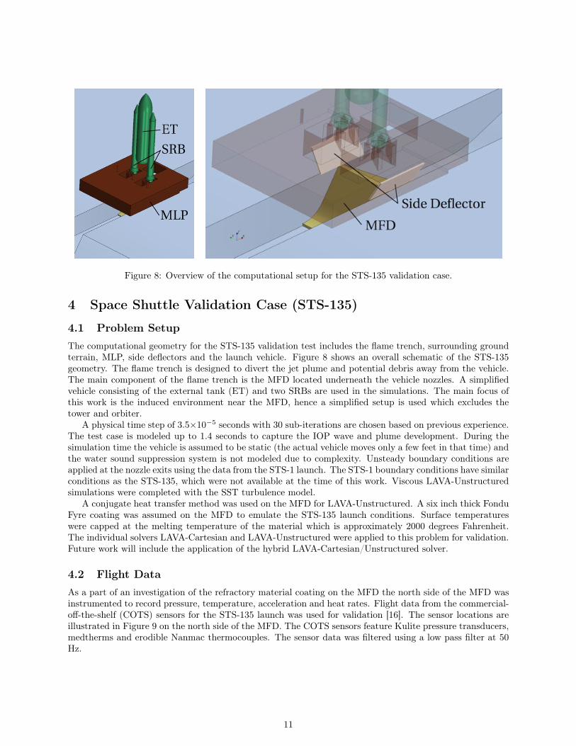
Figure 8: Overview of the computational setup for the STS-135 validation case.

4 Space Shuttle Validation Case (STS-135)

4.1 Problem Setup

The computational geometry for the STS-135 validation test includes the flame trench, surrounding groundterrain, MLP, side deflectors and the launch vehicle. Figure 8 shows an overall schematic of the STS-135geometry. The flame trench is designed to divert the jet plume and potential debris away from the vehicle.The main component of the flame trench is the MFD located underneath the vehicle nozzles. A simplifiedvehicle consisting of the external tank (ET) and two SRBs are used in the simulations. The main focus ofthis work is the induced environment near the MFD, hence a simplified setup is used which excludes thetower and orbiter.

A physical time step of 3.5⇥10�5 seconds with 30 sub-iterations are chosen based on previous experience.The test case is modeled up to 1.4 seconds to capture the IOP wave and plume development. During thesimulation time the vehicle is assumed to be static (the actual vehicle moves only a few feet in that time) andthe water sound suppression system is not modeled due to complexity. Unsteady boundary conditions areapplied at the nozzle exits using the data from the STS-1 launch. The STS-1 boundary conditions have similarconditions as the STS-135, which were not available at the time of this work. Viscous LAVA-Unstructuredsimulations were completed with the SST turbulence model.

A conjugate heat transfer method was used on the MFD for LAVA-Unstructured. A six inch thick FonduFyre coating was assumed on the MFD to emulate the STS-135 launch conditions. Surface temperatureswere capped at the melting temperature of the material which is approximately 2000 degrees Fahrenheit.The individual solvers LAVA-Cartesian and LAVA-Unstructured were applied to this problem for validation.Future work will include the application of the hybrid LAVA-Cartesian/Unstructured solver.

4.2 Flight Data

As a part of an investigation of the refractory material coating on the MFD the north side of the MFD wasinstrumented to record pressure, temperature, acceleration and heat rates. Flight data from the commercial-off-the-shelf (COTS) sensors for the STS-135 launch was used for validation [16]. The sensor locations areillustrated in Figure 9 on the north side of the MFD. The COTS sensors feature Kulite pressure transducers,medtherms and erodible Nanmac thermocouples. The sensor data was filtered using a low pass filter at 50Hz.

11

Figure 9: Experimental instrumentation points for north side of main deflector and an image of COTS sensorconfiguration for STS-135 launch.

Figure 10: Side views of block-structured immersed-boundary Cartesian volume grid for STS-135 test case.

4.3 Computational Grids

Using the LAVA framework, structured and unstructured computational grids were generated for the STS-135 geometry.

4.3.1 Block-Structured Cartesian Grid

Cartesian mesh generation for LAVA-Cartesian requires only a closed water-tight triangulation as input andautomatically produces an immersed-boundary Cartesian mesh. User input can be used to customize thelocal refinement through either solution gradients, entropy adjoint or geometric features (e.g. componenttagging, edge tagging and regions of interest) for a high degree of control. To fully resolve the plumeimpingement on the MFD, a seven level Cartesian grid was generated. The finest level has a spacing of 3.9cm to accurately capture the unsteady boundary conditions at the nozzle exits. Regions of interest are usedto cluster points underneath the nozzle and in the vicinity of the MFD. The grid is illustrated in Figure10 along x=0 and y=0 slices. Domain boundaries are set to approximately 450 meters in each direction toavoid reflections off the outer boundaries. The grid consists of 76 million cells in the full domain.

12

Figure 11: Polygon surface mesh for unstructured grid with MLP hidden for STS.

Figure 12: Side view of unstructured prismatic/polyhedral volume grid for STS-135 test case.

4.3.2 Unstructured Grid

The commercial software, STARCCM+ [17], was used to generate the unstructured grid from the surfacetriangulations. The quality of the unstructured grid is highly dependant on the surface grid, which dictatesthe resolution of the volume mesh. With the main focus on the trench and plume impingement, higherresolution is applied on the MFD and plume region. A spacing of 0.15 m is applied on the MFD and insidethe MLP exhaust holes. Figure 11 shows the surface mesh with the MLP hidden.

Prismatic boundary layer grids were used near the regions of interest (MFD) and a polyhedral mesh wasused to fill the remaining domain. Special care was taken to maintain high fidelity in the plume region. Thegrid is designed to become coarse in the farfield to avoid reflections at the boundaries. A volume specificationis used to maintain an edge length of approximately 0.15 m in the plume impingement region. Additionalrefinement is placed near the nozzle exits to accurately resolve the unsteady boundary conditions. Theprismatic grid has a wall spacing of 2.0⇥10�6 and has approximately 57 layers with a stretching ratio of 1.2to smoothly interface with the polyhedral mesh. These grid parameters follow from the best practices of the2D trench problem. The grid consists of 6.12 million cells and 1.29 million faces (Figure 12).

13

Figure 13: Instantaneous pressure distribution (PSIG) at several times using LAVA-Cartesian

4.4 Results: Pressure Environment

With the unsteady ignition of the SRBs, a large ignition over pressure is generated followed by the impinge-ment of the plume on the MFD. Throughout the development of the flow, multiple shocks are generated onthe MFD as the supersonic flow is deflected. This leads to multiple regions of high pressure (impingementpoints) and low pressure (recirculation points) as the plume develops. To visualize the behavior of thisflow field, the gauge pressure distribution (PSIG) is plotted on the surface of the trench in Figure 13 fromthe LAVA-Cartesian simulation. The time steps are chosen such that the first image illustrates the initialimpingement of the plume, flow passing the north side step in the MFD, partially developed flow and in thelast image the quasi-steady full thrust conditions. In the initial flow field, the ignition of the SRBs impactsthe MFD and disperses along the trench. As the flow develops a distinct shock structure is generated at thecurved region of the MFD. Furthermore, with both SRB plumes deflected to the north side of the trench theflow is contained between the trench walls and the opposing SRB plumes.

To visualize the complexity and unsteadiness of the flow field the mass fractions from multi-species LAVA-Cartesian results are shown in Figure 14. Three levels are shown: 95, 50 and 25 percent exhaust gas massfractions. The 95 percent exhaust gas mass fraction is an indicator of where the majority of the exhaustgas is directed. At the later time sequences, the shear layer instabilities and energetic flow leads to mixing

14

Figure 14: Isosurfaces of exhaust mass fraction at several time sequences using LAVA-Cartesian. Redindicates 95% exhaust gas, yellow is 50% and white is 25%. For better visibility the MLP is shown astransparent.

and reduced concentrations of pure exhaust gas. These plots are also indicators of plume containment of thetrench side walls and MFD. The results indicate the plume is well contained inside the trench and becomeshighly unsteady away from the MFD.

The interaction of the two plumes with the MFD and trench leads to a complex and unsteady pressureenvironment. A key aspect of this work is to investigate the required fidelity to accurately predict thepressure environment of this flow field. The LAVA-Cartesian results are obtained by solving the inviscidEuler equations due to the computational advantages of the approach. Inviscid physics dominate the flow,due to the fact that within the nozzle and along the body the boundary layers are generally thin [18]. Alsothe large density gradients in the flow field lead to shear layer instabilities and growth of Kelvin-Helmholtz

15

(a) LAVA-Cartesian Multi-Species

(b) LAVA-Cartesian Single Gas

(c) LAVA-Unstructured Viscous Single Gas

Figure 15: Gauge pressure distributions (PSIG) with white sonic-line contours are shown in the left columnwith Mach number distributions on the right column at the quasi-steady state full thrust time of t=0.7seconds. From the top to the bottom: (a) inviscid multi-species, (b) inviscid single gas and (c) viscous singlegas.

instability characteristics to the jets [19] which we modelled with the SST turbulence model in the LAVA-Unstructured code. To illustrate this, the pressure and Mach number distributions are shown in Figure 15for LAVA-Cartesian multiple species and single gas as well as single gas LAVA-Unstructured simulations.

The results are taken at the quasi-steady state full thrust conditions (t=0.7 seconds) with the contourlevels of the Mach number set from 0 to 4.2 and the pressure contour range from -10 to 70 PSIG. Sonic lines are

16

(a) Flight Data (b) Simulation Data

Figure 16: Unsteady pressure history at top sensor location on MFD. Raw flight data (maroon �), filteredflight data (black �), LAVA-Unstructured viscous (blue �) and LAVA-Cartesian inviscid (red �) are shown.

also shown in the PSIG distribution plots to visualize the shock structure on the MFD. The first observationof the results is that the major structures are consistent between each modeling fidelity level. Mach coneswithin the jet are sharply defined and the strong shock at the first impingement point are captured. Asidefrom the higher jet spreading rate, partially due to turbulent mixing, the viscous and inviscid results areconsistent. Similarly, the single gas and multi-species results have nearly identical pressure values and shockstructures. The results indicate single gas inviscid simulations are sufficient in capturing the MFD pressureenvironment for these flow fields.

For a quantitative comparison, unsteady pressure probe data was accumulated for the simulation dataand flight data. As shown in Figure 9, three locations (bottom, middle and top) were examined on the MFD.Figure 16 shows the unsteady pressure history for the inviscid multi-species, viscous single-species and boththe raw and filtered flight data. Comparison of the simulation data to the flight data at the top sensorreveals an approximately 0.1 second phase lag. The source of the phase lag can be primarily attributedto neglecting the multi-phase effects of the water sound suppression system which would slow the plumepropagation speed. Another potential cause of the time lag is differences in the ramping of the STS-1 andSTS-135 engine conditions. Small discrepancies in the unsteady pressure ramping has the potential to changethe plume characteristics. The numerical simulations also do not account for the multi-phase flow and thefact that waves propagate at different speeds in different mediums. However, the more important aspect ofthe comparison is the pressure peaks and the data trends. On those fronts, the simulation data shows goodagreement in capturing the initial IOP and reduction in pressure. Good agreement is also evident betweenthe inviscid and viscous simulation results, consistent with the previous pressure and Mach results. Note,the unfiltered pressure sensor flight data contains high frequency content that is eliminated with filtering.

Similar behavior is observed at the middle and bottom sensor location shown in Figure 17 and 18 respec-tively. Here the different numerical simulations are in good agreement with each other and capture the IOPand pressure signatures. The median value of the flight data appears to be slightly lower, which again canbe attributed to the water sound suppression system dampening the pressure field. The unfiltered pressuresensor flight data exhibits a similar IOP pressure amplitude as the simulation data, which is not true of thefiltered flight data.

17

(a) Flight Data (b) Simulation Data

Figure 17: Unsteady pressure history at middle sensor location on MFD. Raw flight data (maroon �), filteredflight data (black �), LAVA-Unstructured viscous (blue �) and LAVA-Cartesian inviscid (red �) are shown.

(a) Flight Data (b) Simulation Data

Figure 18: Unsteady pressure history at bottom sensor location on MFD. Raw flight data (maroon �),filtered flight data (black �), LAVA-Unstructured viscous (blue �) and LAVA-Cartesian inviscid (red �) areshown.

4.5 Results: Thermal Environment

The thermal environment plays a critical role in the safety and design of the launch site. In particular, thermalprotection on the MFD is designed to withstand the high pressure and temperatures of the impinging jetfor multiple launches. Insufficient thermal protection can lead to damage of the trench and the potential fordebris which may harm the vehicle. Unlike the pressure environment, where inviscid features dominate theflow, viscous simulations are required to accurately capture the viscous heating at the wall. The proposedapproach is to use the viscous turbulent capabilities of LAVA-Unstructured with a conjugate heat transfermethodology to approximate wall heating effects. To visualize the thermal environment, the temperaturedistribution is shown on the MFD in Figure 19.

Comparison of the temperature and heat rate distributions with the pressure distributions (Figure 13)shows the correlation between high pressure and temperature regions. Near the first impingement point (topsensor) the surface temperature reaches a local maximum. A strong shock develops on the curved region ofthe MFD leading to a second impingement point. Along the shock, the temperature field indicates a highertemperature and heat rate region. The point sensors are also superimposed on the plot to give a sense of the

18

t=0.231 s

t=0.602 s

Figure 19: Instantanous temperature distribution (�F) and heat rate (BTU/(ft2s)) at multiple time sequencesusing LAVA-Unstructured on the north side of the MFD. The sensor locations are superimposed on thesurfaces as white squares.

flow field around sensor locations. The upper sensor is located in the high temperature plume impingementlocation while the middle temperature sensor is on the edge of the region. For the lower sensor, the flowappears to be in the relatively colder spot between the upper and lower impingement locations.

A comparison of the unsteady temperature and heat rate are shown in Figure 20 for the viscous singlegas simulation of LAVA-Unstructured and flight medtherm data. The results display the same 0.1 secondtime delay seen in pressure but shows good agreement otherwise. A large gradient in temperature is visibleas the plume impinges on the MFD followed by multiple rises and plateaus. The simulation data reachesthe specified melting point temperature limit at a faster rate than the flight data. The discrepancy canbe associated with the water sound suppression system reducing surface temperatures. Furthermore, themedtherm sensors are set in stainless steel castings while the numerical simulations place them directly inFondu Fyre. The lower heat capacitance of the stainless steel contributes to the lower temperature rise.Figure 20b shows a good comparison between the heat rate flight data. A large initial spike in heat rateoccurs at the initial impingement and reaches a quasi-steady state value. The flight data show significantspikes in heat rate which can be associated with particle heating.

Similar temperature and heat rate comparisons are shown in Figure 21 for the middle sensor location.The temperature history of the simulation results show a similar trend to the flight data but reach meltingtemperature at a faster rate. An initial spike is shown followed by multiple small spikes as the flow developsthese are evident in both the simulation and flight data. The heat rate also shows a large spike during theinitial impingement and reaches a semi-steady value of approximately 300 BTU/(ft2s). The simulation data

19

(a) (b)

Figure 20: Unsteady temperature (a) and heat rate (b) history at top sensor location on MFD. Flight data(black �) and LAVA-Unstructured (blue �) are shown.

(a) (b)

Figure 21: Unsteady temperature (a) and heat rate (b) history at middle sensor location on MFD. Flightdata (black �) and LAVA-Unstructured (blue �) are shown.

shows a similar trend but has a higher mean value. The significant drop in the flight heat rate data at 1.6seconds is indicative of sensor failure. Figure 22 shows the temperature and heat rate comparison for thebottom sensor. Both the simulation temperature and heat rate are conservative estimates of the flight dataresults. Overall, results indicate the viscous single gas has similar trends as the flight data.

20

(a) (b)

Figure 22: Unsteady temperature (a) and heat rate (b) history at bottom sensor location on MFD. Flightdata (black �) and LAVA-Unstructured (blue �) are shown.

5 Conclusion and Future Work

Progress towards hybrid simulations of the launch environment has been made with the application of LAVA-Cartesian/Unstructured on a 2D trench test case and validation of the individual solvers on a Space Shuttletest case (STS-135). Pressure signatures for the 2D trench case indicated that single gas simulations areadequate while code-to-code comparisons were positive for the hybrid approach in terms of pressure andtemperature. The individual flow solvers, LAVA-Cartesian and LAVA-Unstructured, were validated againstflight data for the Space Shuttle test case and showed good agreement. The pressure environment was re-solved with both LAVA-Cartesian inviscid simulations and LAVA-Unstructured viscous simulations. Pressureamplitudes for the IOP and trends in flight data were captured with both approaches. With the conjugateheat transfer method, temperature and heat rate data from LAVA-Unstructured showed conservative com-parisons. Application of the hybrid approach to the Space Shuttle test case is currently underway, as well asa study of the sensitivity of thermal results to material properties. The hybrid grid coupling framework thathas been established shows the potential to reduce grid generation time, improve simulation turn-aroundtime and adequately model the launch environment for design analysis.

6 Acknowledgements

This work has been partially been funded by the 21st Century Launch Complex. We would also like to thankDr. Bruce Vu and Dr. Christopher R. Parlier for providing STS-135 flight data.

References

[1] R. L. Evans and O. L. Sparks. Launch deflector design criteria and their appication to the Saturn C-1deflector. Technical Note d-1275, NASA, 1963.

[2] C. Kiris, J. Housman, M. Gusman, W. Chan, and D. Kwak. Time-Accurate Computational Analysis ofthe Flame Trench Applications. In 21st Intl. Conf. on Parallel Computational Fluid Dynamics, pages37–41, 2009.

[3] R.H. Nichols and P.G. Buning. User’s Manual for OVERFLOW 2.1. Version 2.1t, August 2008.[4] W. Chan, R.J. Gomez, S. Rogers, and P. Buning. Best Practices in Overset Grid Generation. In 32nd

AIAA Fluid Dynamics Conference and Exhibit, St. Louis, Missouri, Jun 24-26 2002. AIAA–2002–3191.[5] S. Pandya, W. Chan, and J. Kless. Automation of Structured Overset Mesh Generation for Rocket

21

Geometries. In 19th AIAA Computational Fluid Dynamics Conference, San Antonio, Texas, Jun 22–252009. AIAA–2009–3993.

[6] M. J. Berger and P. Colella. Local adaptive mesh refinement for shock hydrodynamics. J. Comput.Phys., 82(1):64–84, May 1989.

[7] A. S. Almgren, J. B. Bell, P. Colella, L. H. Howell, and M. L. Welcome. A conservative adaptiveprojection method for the variable density incompressible Navier-Stokes equations. J. Comp. Phys.,142:1–46, 1998.

[8] M. F. Barad and P. Colella. A Fourth-Order Accurate Local Refinement Method for Poisson’s Equation.J. Comp. Phys., 209(1):1–18, October 2005.

[9] M. F. Barad, P. Colella, and S. G. Schladow. An Adaptive Cut-Cell Method for Environmental FluidMechanics. Int. J. Numer. Meth. Fluids, 60(5):473–514, 2009.

[10] Q. Zhang, H. Johansen, and P. Colella. A fourth-order accurate finite-volume method with structuredadaptive mesh refinement for solving the advection-diffusion equation. SIAM Journal on ScientificComputing, 34(2):B179–B201, 2012.

[11] P. Colella, D. T. Graves, T. J. Ligocki, D. F. Martin, D. Modiano, D. B. Serafini, and B. Van Straalen.Chombo Software Package for AMR Applications - Design Document. unpublished, 2000.

[12] R. Mittal, H. Dong, M. Bozkurttas, F.M. Najjar, A. Vargas, and A. von Loebbecke. A versatile sharpinterface immersed boundary method for incompressible flows with complex boundaries. Journal ofComputational Physics, 227(10):4825 – 4852, 2008.

[13] S.R. Spalart and S.A. Allmaras. A One-Equation Turbulence Model for Aerodynamic Flows. In 30thAerospace Sciences Meeting and Exhibit, Reno, NV, January 1992. AIAA–92–0439.

[14] F.R. Menter. Zonal Two Equation k-! Turbulence Models For Aerodynamic Flows. In 23rd FluidDynamics, Plasmadynamics, and Lasers Conference, Orlando, FL, July 1993. AIAA–93–2906.

[15] J. Housman, M. Barad, and C. Kiris. Space-time accuracy assessment of cfd simulations for the launchenvironment. In 29th AIAA Applied Aerodynamics Conference, June 2011. AIAA-2011-3650.

[16] C. R. Parlier. Pad A main flame deflector sensor data and evaluation. In 2011 Thermal and FluidsAnalysis Workshop (TFAWS2011), Aug 15–19 2011.

[17] CD-Adapco. Star-ccm+ version 4.02.011 user guide, 2008.[18] M. L. Norma and K.-H. A. Winkler. Supersonic jets. Los Alamos Science, Sping/Summer:38–71, 1985.[19] C. K. W. Tam, N. N. Pastouchenko, and K. Viswanathan. Fine-scale turbulence noise from hot jets.

AIAA Journal, 43, 2005.

22