Towards Accurate Numerical Method for Monodomain Models Using

a Realistic Heart Geometry

Youssef Belhamadia

University of Alberta,

Campus Saint-Jean,

Edmonton, Alberta, Canada.

Andre Fortin

Universite Laval,

Departement de mathematiques et de statistique,

Quebec, Quebec, Canada

Yves Bourgault

University of Ottawa,

Department of Mathematics and Statistics,

Ottawa, Ontario, Canada.

April 20, 2009

Paper to be submitted to: Mathematical Biosciences

Corresponding author: youssef.belhamadia@ualberta.ca

1

Abstract

The simulation of cardiac electrophysiological waves are known to require extremely fine meshes, lim-

iting the applicability of current numerical models to simplified geometries and ionic models. In this

work, an accurate numerical method based on a time-dependent anisotropic remeshing strategy is pre-

sented for simulating three-dimensional cardiac electrophysiological waves. The numerical proposed

method greatly reduces the number of elements and enhances the accuracy of the prediction of the

electrical wave fronts. Illustrations of the performance and the accuracy of the proposed method are

presented using a realistic heart geometry. Qualitative and quantitative results shows that the proposed

methodology is far superior to the uniform mesh methods commonly used in cardiac electrophysiology.

Keywords : Monodomain model, finite element method, anisotropic mesh adaptation, cardiac elec-

trophysiology, FitzHugh-Nagumo and Aliev-Panfilov ionic models.

1 Introduction

Knowledge of the electrical activity of the myocardium is essential to treat heart diseases and to un-

derstand rhythm disorders of the heart. Numerical modeling plays a crucial role and provides the

necessary tools for understanding normal and abnormal cardiac electrical activity. However, accurate

simulation of three-dimensional electrical waves in the human heart is not yet feasible. The major

difficulty is that the action potential is a wave with sharp depolarization and repolarization fronts.

This wave travels across the whole myocardium, calling for grids that are uniformly fine over the whole

computational domain. Indeed coarse grids lead to wrong propagation speed and wave trajectories (see

Bourgault et al. [8]). Several authors estimate that a typical simulation of the whole heart may require

about 107 grid points (see Cherry et al. [9] and Ying [50]). Given that several unknowns are attached

to each grid point (some of the latest ionic models contains 30 to 60 variables as presented in Panfilov

2

and Holden [36, chapter 1]), numerical simulations using uniform meshes for a realistic heart geometry

are beyond or at least at the limit of the existing computational resources.

To overcome these difficulties, many methods have been developed in the literature. Parallel com-

puting techniques are used to reduce the computational time at each time step when a fixed spatial

mesh is used (see Colli Franzone and Pavarino [11], Karpoukhin et al. [27] and Weber dos Santos et

al. [49]). Several time-stepping strategies have also been used, including explicit (Hooke et al. [26],

Penland et al. [37], and Roth [40]), fully implicit (Bourgault et al. [8], Hooke et al. [26], and Murillo

and Cai [32]), semi-implicit (Colli Franzone and Pavarino [20], Hooke et al. [26], Keener and Bogar [28],

Pennacchio and Simoncini [38], Bourgault and Ethier [16]) and operator-splitting (Lines et al. [29, 30],

Weber dos Santos et al. [48], Sundnes [43]) methods. Explicit methods are inexpensive in terms of mem-

ory use and computational time at each time step, but they suffer from strong limitations on the time

step ∆t to ensure the stability of the solution. On the other hand, semi-implicit and operator-splitting

methods are not as stringent on the time step and permit the use of different solution techniques for

the nonlinear terms, such as the ionic currents, and the rest of the governing equations. For example,

Sundnes et al. [44] and Vigmond et al. [47] used different time-stepping schemes for the ionic models

and the governing partial differential equations.

Recently, mesh adaptation methods have been introduced to capture moving front since it is ex-

tremely helpful to improve the accuracy of finite element simulations (see Fortin and Belhamadia [18],

Fortin and Benmoussa [19], and Alauzet et al. [2]). The technique consists in locating finer mesh cells

near the front position while a coarser mesh is used away from the front, resulting in a much smaller

total number of mesh cells to achieve a given accuracy compared to uniform meshes. In the context

of simulating the cardiac electrical activity, a generalized finite difference method using irregular com-

putational meshes is used in Trew et al. [46], while an adaptive finite element method in both space

3

and time in two and three dimensions is presented in Cherry et al. [9], Colli Franzone et al. [10] and

Trangenstein and Kim [45]. The previous work on the adaptive method uses unstructured computa-

tional meshes including only refinement/coarsening and isotropic cells. However, to our knowledge,

three-dimensional anisotropic mesh adaptation, where cells are not only refined but also elongated

along a specified direction, is not yet introduced for simulating the cardiac electrophysiological activ-

ity, which is the scope of the this paper.

The main purpose of this paper is to develop and show the efficiency of an anisotropic time-

dependent adaptive method for accurately computing time-evolving electrical waves in a 3-D proto-

type geometry of the human heart at a much smaller cost than current uniform grid methods. The

method proposed reduces greatly the size of the spatial mesh as well as the computational time. Also,

an accurate prediction of the depolarization and repolarization fronts is obtained showing the advan-

tages of the proposed method. A two-dimensional adaptive strategy based on the hierarchical error

estimator has been presented in Belhamadia [5]. It was clearly shown that anisotropic meshes are

necessary to determine evolving depolarization and repolarization fronts. In this paper, a different

error estimator is used, which is based on the definition of edge length using a solution dependent met-

ric. For more details about the metric error estimator, the reader is referred to Habashi et al. [23, 1, 14].

Two categories of mathematical models exist for simulating cardiac electrophysiological waves. The

first category consists in using the so-called bidomain model. This model is a system of two nonlinear

partial differential equations, one for each of the intra- and extra-cellular potentials, coupled to a sys-

tem of ordinary differential equations representing the cell ionic activity (see Bourgault et al. [8], Colli

Franzone et al. [12], and Roth [39]). Although the bidomain model gives an accurate representation

of electrophysiological waves in the myocardium and is capable of reproducing the electrocardiogram

(ECG) by coupling the heart with the thorax, a second category of simplified mathematical models

4

consist in modelling only the trans-membrane potential. This reduces the bidomain model to a mon-

odomain model with a single nonlinear partial differential equations, coupled with the same system of

ordinary differential equations for the ionic activity. This model is widely studied and describes the

dynamic of a general excitable cardiac tissue, at the expense of limited capabilities in reproducing the

ECG. For more details on the various models, the reader is referred to Colli Franzone et al. [13] and

Ying [50] .

The adaptive method developed in this paper, is general and could be used both for the mono- and

bi-domain models. As a proof of concept though, this paper will focus on the most commonly used

monodomain model with relatively simple ion kinetics, namely the well-known FitzHugh-Nagumo (see

FitzHugh [17] and Nagumo et al. [33]) and Aliev-Panfilov models (see Aliev and Panfilov [3]).

This paper is organized as follows. Section 2 presents a brief description of the monodomain model

with FitzHugh-Nagumo and Aliev-Panfilov ion kinetics. Also, the weak formulation and finite element

discretization for the monodomain models are presented. Section 3 is devoted to a description of

the adaptive strategy while the last section presents three-dimensional numerical results. A realistic

geometry of the heart is used showing the performance and the accuracy of the anisotropic mesh

adaptation method.

2 Mathematical Model

Although the adaptive method proposed in this work would be the same for complex electrophysiological

models, this paper treats the most commonly used monodomain model, and simple FitzHugh-Nagumo

and Aliev-Panfilov ion kinetics. These models consist of a nonlinear partial differential equation for the

transmembrane potential U coupled with an ordinary differential equation for the recovery variable V .

5

This ordinary differential equation and the associated variable V mimic the slow ionic behavior of the

myocardium cell membranes, “slow” compared to the fast dynamics of the transmembrane potential

U . The monodomain used in this work takes the following form:

∂U

∂t= ∇ · (D∇U) + Iion(U, V ) + Is,

∂V

∂t= G(U, V ).

(1)

where Is is the current due to an external stimulus, Iion(U, V ) the total ionic current across the mem-

branes andG(U, V ) represents the time derivative of a lumped gating variable. Both functions Iion(U, V )

and G(U, V ) depend on the ionic model, with at least Iion(U, V ) taken as a nonlinear function of U .

The first ionic model was introduced by Hodgkin and Huxley in 1952. Their model describes in-

dividual currents for K+ and Na+ ions and a leaking current crossing the cell membrane of giant

squid axons (see Hodgkin and Huxley [25]). Ionic models were later specialized to cardiac cells (see

[36, chapter 1] for a review and references). Modern cardiac ionic models include more ionic currents

and gating variables, resulting generally in a set of 10 to 60 ordinary differential equations. How-

ever, simplified “two-variable” models have been developed that aim at reproducing the shape of the

trans-membrane potential at the cellular level without reproducing the detailed ion kinetics, the most

famous representative of which models being proposed by FitzHugh [17] and Nagumo et al. [33] in

1961. This gives rise to the so-called FitzHugh-Nagumo model qualitatively reproducing the action

potential with two variables. In 1996 Aliev-Panfilov model was introduced to reproduce more realistic

shapes of the cardiac action potential and to reproduce the APD restitution characteristic observed

in the experiments (see Aliev and Panfilov [3]). In this paper, FitzHugh-Nagumo and Aliev-Panfilov

models are used to illustrate the adaptive method, which consist on the following equations

• FitzHugh-Nagumo model

6

Iion = kU(U − a)(1− U)− V, and G(U, V ) = ε(γU − βV ).

• Aliev-Panfilov model

Iion = kU(U − a)(1− U)− UV, and G(U, V ) =(ε+

µ1V

µ2 + U

)(−V − kU(U − a− 1)) .

All the parameters including the time t are dimensionless and will be set in the numerical simulation

section. Although FitzHugh-Nagumo and Aliev-Panfilov models use dimensionless units, the simula-

tions results could be compared to experimental studies. For instance, according to experimental results

presented in Elharrar and Surawicz [15] each non-dimensional time unit corresponds to 12.9ms in the

Aliev-Panfilov model, and the actual transmembrane potential is recovered by E[mV ] = −80 + 100U .

For more details the reader is refereed to Nash and Panfilov [35].

The variational formulation of the system of nonlinear equation (1) is straightforward and obtained

by multiplying this system by test functions (φ, ψ) and integrating by parts the second order terms.

The solution (U, V ) = (U(t), V (t)) satisfies the following variational equation

∫Ω

∂U

∂tφ dΩ +

∫Ω

D∇U ·∇ φ dΩ =∫

Ω(f(U, V ) + Is) φ dΩ

∫Ω

∂V

∂tψ dΩ =

∫ΩG(U, V ) ψ dΩ.

(2)

for all (φ, ψ) in an appropriate function space (which depends also on the boundary conditions on ∂Ω).

In all our numerical simulations, quadratic (P2) finite elements and a fully implicit backward sec-

ond order scheme (known as Gear or BDF2 in the literature) are employed for the spatial and time

discretizations, respectively. For instance, given approximate solutions Un−1, Un and Un+1 at times

tn−1, tn and tn+1, respectively, the time derivative at time tn+1 is approximated by:

7

∂U

∂t(t(n+1)) ' 3U (n+1) − 4U (n) + U (n−1)

2∆t.

The variational formulation or finite element method then reads as: Find U (n+1), V (n+1) such that

∫Ω

3U (n+1) − 4U (n) + U (n−1)

2∆tφ dΩ +

∫Ω

D∇U (n+1) ·∇ φ dΩ =∫

Ω(f(U (n+1), V (n+1)) + Is) φ dΩ

∫Ω

3V (n+1) − 4V (n) + V (n−1)

2∆tψ dΩ =

∫ΩG(U (n+1), V (n+1)) ψ dΩ.

(3)

for all test functions (φ, ψ).

The reader is refereed to Belhamadia [5] for more details about a comparison between different

time-stepping schemes and spatial dicretizations. The system (3) is nonlinear. Newton’s method was

used to solve this system at each time step and few iterations were needed to get a residual norm

of 10−6. The linear formulation resulting from Newton’s method requires the solution of huge linear

systems. Direct solvers such as Gaussian elimination are not appropriate since the number of mesh

elements required for electrical wave fronts is huge. Iterative methods, such as the GMRES solver [41]

with an incomplete LU decomposition (ILU) as preconditionners from the PETSc library [4], turned

out to be more suitable from both memory space and CPU time point of views.

3 Adaptive Method

In this work, an adaptive time dependent algorithm was developed for simulating time-evolving car-

diac electrophysiological waves. There are several types of the error estimator that could be used to

control the error made on an exact solution. In Belhamadia [5], a hierarchical error estimator was used

for the solution of two-dimensional electrical waves of the heart. Its extension to three-dimensional

8

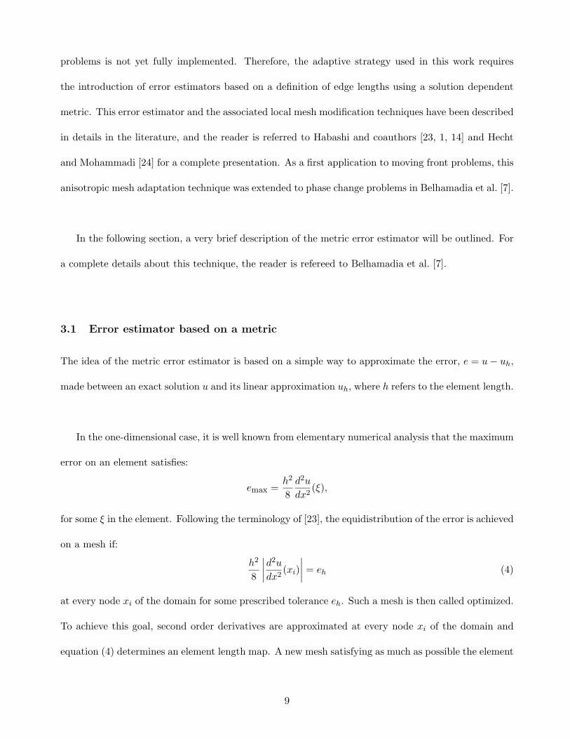
problems is not yet fully implemented. Therefore, the adaptive strategy used in this work requires

the introduction of error estimators based on a definition of edge lengths using a solution dependent

metric. This error estimator and the associated local mesh modification techniques have been described

in details in the literature, and the reader is referred to Habashi and coauthors [23, 1, 14] and Hecht

and Mohammadi [24] for a complete presentation. As a first application to moving front problems, this

anisotropic mesh adaptation technique was extended to phase change problems in Belhamadia et al. [7].

In the following section, a very brief description of the metric error estimator will be outlined. For

a complete details about this technique, the reader is refereed to Belhamadia et al. [7].

3.1 Error estimator based on a metric

The idea of the metric error estimator is based on a simple way to approximate the error, e = u− uh,

made between an exact solution u and its linear approximation uh, where h refers to the element length.

In the one-dimensional case, it is well known from elementary numerical analysis that the maximum

error on an element satisfies:

emax =h2

8d2u

dx2(ξ),

for some ξ in the element. Following the terminology of [23], the equidistribution of the error is achieved

on a mesh if:

h2

8

∣∣∣∣d2u

dx2(xi)

∣∣∣∣ = eh (4)

at every node xi of the domain for some prescribed tolerance eh. Such a mesh is then called optimized.

To achieve this goal, second order derivatives are approximated at every node xi of the domain and

equation (4) determines an element length map. A new mesh satisfying as much as possible the element

9

length map is then produced and a new solution is computed.

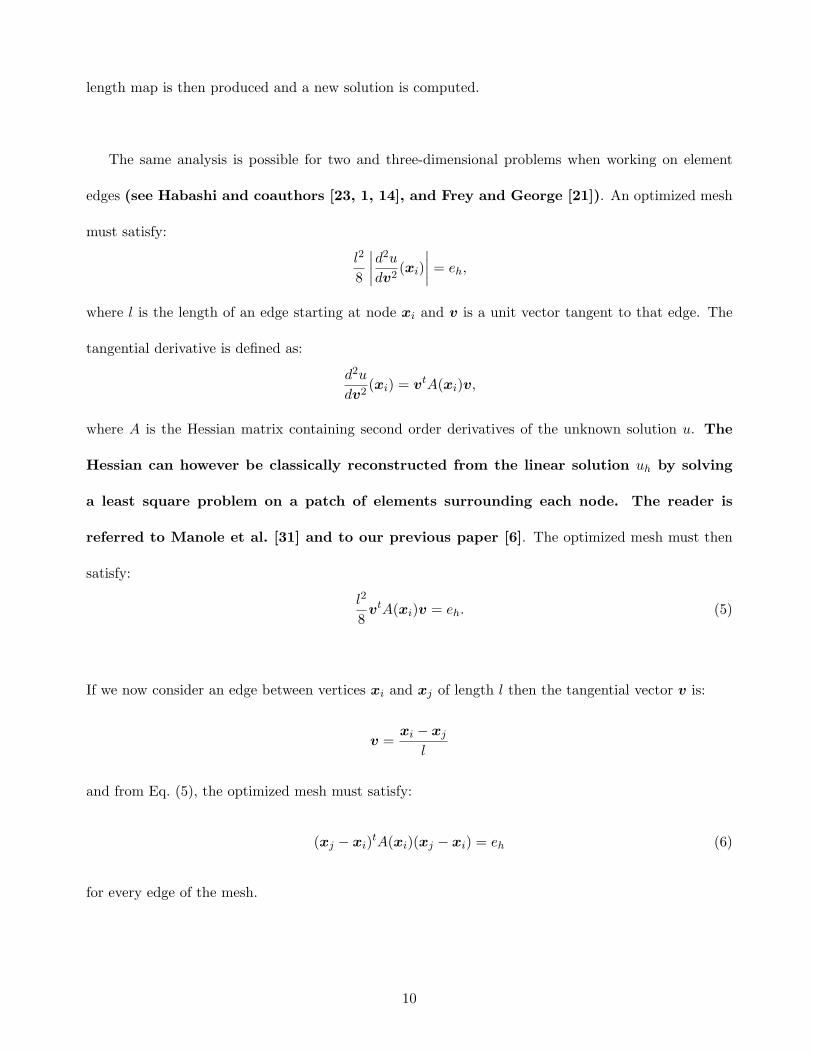
The same analysis is possible for two and three-dimensional problems when working on element

edges (see Habashi and coauthors [23, 1, 14], and Frey and George [21]). An optimized mesh

must satisfy:

l2

8

∣∣∣∣d2u

dv2(xi)

∣∣∣∣ = eh,

where l is the length of an edge starting at node xi and v is a unit vector tangent to that edge. The

tangential derivative is defined as:

d2u

dv2(xi) = vtA(xi)v,

where A is the Hessian matrix containing second order derivatives of the unknown solution u. The

Hessian can however be classically reconstructed from the linear solution uh by solving

a least square problem on a patch of elements surrounding each node. The reader is

referred to Manole et al. [31] and to our previous paper [6]. The optimized mesh must then

satisfy:

l2

8vtA(xi)v = eh. (5)

If we now consider an edge between vertices xi and xj of length l then the tangential vector v is:

v =xi − xj

l

and from Eq. (5), the optimized mesh must satisfy:

(xj − xi)tA(xi)(xj − xi) = eh (6)

for every edge of the mesh.

10

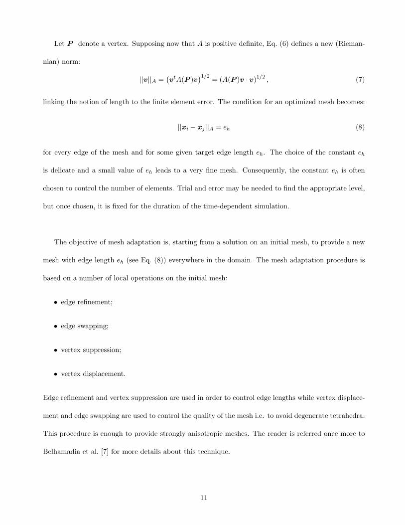
Let P denote a vertex. Supposing now that A is positive definite, Eq. (6) defines a new (Rieman-

nian) norm:

||v||A =(vtA(P )v

)1/2 = (A(P )v · v)1/2 , (7)

linking the notion of length to the finite element error. The condition for an optimized mesh becomes:

||xi − xj ||A = eh (8)

for every edge of the mesh and for some given target edge length eh. The choice of the constant eh

is delicate and a small value of eh leads to a very fine mesh. Consequently, the constant eh is often

chosen to control the number of elements. Trial and error may be needed to find the appropriate level,

but once chosen, it is fixed for the duration of the time-dependent simulation.

The objective of mesh adaptation is, starting from a solution on an initial mesh, to provide a new

mesh with edge length eh (see Eq. (8)) everywhere in the domain. The mesh adaptation procedure is

based on a number of local operations on the initial mesh:

• edge refinement;

• edge swapping;

• vertex suppression;

• vertex displacement.

Edge refinement and vertex suppression are used in order to control edge lengths while vertex displace-

ment and edge swapping are used to control the quality of the mesh i.e. to avoid degenerate tetrahedra.

This procedure is enough to provide strongly anisotropic meshes. The reader is referred once more to

Belhamadia et al. [7] for more details about this technique.

11

3.2 Time-dependent adaptive algorithm

The adaptive time-dependent meshing strategy for accurately simulating moving three-dimensional

action potentials is now presented. The objective of this method is to build at each time step tn a fine

mesh in all regions where the variables U and V evolve, and a coarse mesh in these other regions with

limited variations of all the model variables. In particular, the mesh must be refined at each time step

near the depolarization/repolarization fronts where steep variation of the transmembrane potential U

and recovery variable V occurs while coarser mesh are sufficient away from these two fronts. Therefore,

the mesh size is greatly reduced at each time step and an accurate solution is obtained.

The overall adaptive strategy is the following:

1. Start from the solutions U (n−1), U (n), V (n−1) and V (n) and a mesh M(n) at time t(n);

2. Solve the system (3) on mesh M(n) to obtain a first approximation of the solutions (denoted

U (n+1) and V (n+1)) at time t(n+1);

3. Adapt the mesh starting from the meshM(n) and the solution dependent metric calculated with

the solution time-variations3U (n+1) − 4U (n) + U (n−1)

2and

3V (n+1) − 4V (n) + V (n−1)

2to obtain

a new mesh M(n+1);

4. Reinterpolate U (n−1), U (n), V (n−1) and V (n) on mesh M(n+1);

5. Solve the system (3) on mesh M(n+1) for Un+1 and V n+1.

6. Next time step: go to step 2.

The mesh is thus adapted at each time step in order to preserve the accuracy of the solutions. To

control the number of elements, a target edge length eh should be chosen by the user, small values of

eh leading to a very fine mesh but very accurate solutions. Once eh chosen, it is fixed for the duration

12

of the time-stepping loop. The ideal adapted mesh at each time step would be such that all edges of

the mesh, calculated using the solution dependent metric, would have this target edge length eh. The

goal of this adaptive method is to build a mesh with nearly equilateral tetrahedra in a Riemannian

metric space.

Since we are using a fully implicit backward second order scheme for time-stepping,

the mesh at a given time step should be able to accurately represent the solutions at

time t(n−1), t(n), and t(n+1), not only at time t(n+1). Ideally, the mesh should be adapted

so that the new mesh can capture the variations of the six functions U (n+1), U (n), U (n−1),

V (n+1), V (n), and V (n−1). In this way, the reinterpolation step (4), which is crutial for an

accurate propagation of the front, gives very good results. Adapting the mesh using six

different error estimators at each time steps would however be extremely costly. The lo-

cal operators used to modify the mesh would have to evaluate if the mesh is appropriate

for each of these six variables. Our experience shows that using a (linear) combina-

tion of the different solutions is a good compromise. In this work, the two functions

3U (n+1) − 4U (n) + U (n−1)

2and

3V (n+1) − 4V (n) + V (n−1)

2were used but recent computations

showed thatU (n+1) + U (n) + U (n−1)

3and

V (n+1) + V (n) + V (n−1)

3also give excellent results.

4 Numerical results

In this section, the performance and robustness of the adaptive method described in the previous sec-

tion will be presented. Three different problems are discussed for this purpose. For the first problem,

a comparison between uniform and adapted meshes in a cubic geometry will be presented. The second

problem is devoted to the numerical simulation of a single electrophysiological wave in a realistic heart

geometry with left and right ventricles (LV and RV, respectively). In this test case, the action potential

13

grows from the apex of the heart. A third problem is done in this same realistic geometry but with

two waves, one would be the action potential naturally growing in the LV while the second wave would

be generated by a pacemaker attached to the RV.

4.1 Cubic geometry

This section is devoted to a qualitative and quantitative comparison of the solutions obtained with

three different uniform meshes with those on adapted meshes. The computational domain is the cube

[0, 100]× [0, 100]× [0, 100]. Homogeneous Neumann conditions are imposed on all sides, and the initial

transmembrane potential U and the recovery variable V are given by:

U(x, t) =

1 if

√(x− 100) + (y − 100) + (z − 100) < 30

0 if√

(x− 100) + (y − 100) + (z − 100) ≥ 30,and V (x, t) = 0.

In the numerical simulations the following values have been used:

FitzHugh-Nagumo model Aliev-Panfilov model

k = 1 k = 8

a = 0.25 a = 0.15

ε = 0.01 ε = 0.002

β = 1 µ1 = 0.2

γ = 0.16875 µ2 = 0.3

D = 1 D = 1

∆t = 5 ∆t = 0.5

To generate uniform meshes, the computational dobmain is divided respectively into 34 992, 82 944,

162 000, and 750 000 tetrahedral elements, which lead respectively to 101 306, 235 298, 453 962, and

14

2 060 602 degrees of freedom since we use quadratic (P2) discretization for both variables U and V .

Figure 1 presents the transmembrane potential using the Aliev-Panfilov model. As can be seen, the

transmembrane potential velocity and front position is sensitive to insufficient mesh resolution. Fig-

ure 2 presents the solution on the adapted mesh using only an average of 59 000 dof which is clearly

almost the same as the one obtained with uniform mesh using 2 060 602 dof. The number of elements

is greatly reduced using the adaptive method since the mesh is refined only in the vicinity of the

front position while keeping sufficient resolution in other regions. The same result is obtained with

FitzHugh-Nagumo model. The! solution using the adapted mesh with only 39 000 dof is comparable

to the solution obtained with the structured mesh using 2060602 dof. Numerical simulations results

for FitzHugh-Nagumo model are similar to Figure 2 and are not presented in this paper to avoid a rep-

etition. In both cases, comparisons of the two numerical solutions with equal accuracy using uniform

and adapted meshes clearly show the advantage of the adaptive method.

Quantitative results are presented in figure 3, in which the transmembrane potential U and the re-

covery variable V at the center of the computational domain are plotted as a function of time using the

uniform and the adapted meshes mentioned above. The results show that the solutions U and V need

a very fine uniform mesh to be properly captured. These solutions on uniform meshes are approaching

the adapted solution at a slow pace when the mesh is refined, but the solutions on the finest uniform

mesh are similar as the adapted solution in spite of the fact that 33 times the number of degrees of

freedom are required on the finest uniform mesh compared to the adapted meshes. Moreover, adaptive

meshing cures the oscillations on the variable U observed near the depolarisation front on the coarser

uniform meshes for the Aliev-Panfilov model (see Figure 3a)).

We next show that our adaptive method properly predicts the depolarization time at the center of

the cube, hence the propagation velocity, by comparing this depolarization time with the asymptotic

15

value computed on uniform meshes as if we were keeping refining these uniform meshes. To do so,

we estimate the depolarization time on finer uniform meshes using Richardson extrapolation. Indeed,

suppose that we want to approximate the time T required for the depolarization front to reach the

center of the computational domain. This depolarization front is here defined as the contour where

U = 0.5 in the depolarization zone. Denote by T (h) the approximate depolarization time obtained on

a mesh of size h. This approximation T (h) is of order 2 since a quadratic finite element method and a

second order time-stepping scheme are used. Assuming that

T = T (h) +O(h2) = T (h) +Ah2 +O(h3)

for some constant A not depending on h, the Richardson extrapolation consists in using two approx-

imations T (h1) and T (h2) for two different values of h, respectively h1 and h2, in order to eliminate

the terms in A and obtain an third order approximation of T . It is straightforward to verify that

T =h2

2T (h1)− h21T (h2)

h22 − h2

1

+O(h3).

The Richardson extrapolate for T is defined as Rh2h1 = h22T (h1)−h2

1T (h2)

h22−h2

1. In cases where the extrapola-

tion works well, an accurate estimate of T is obtained as if a very fine mesh was used to compute the

solution and obtain T (h).

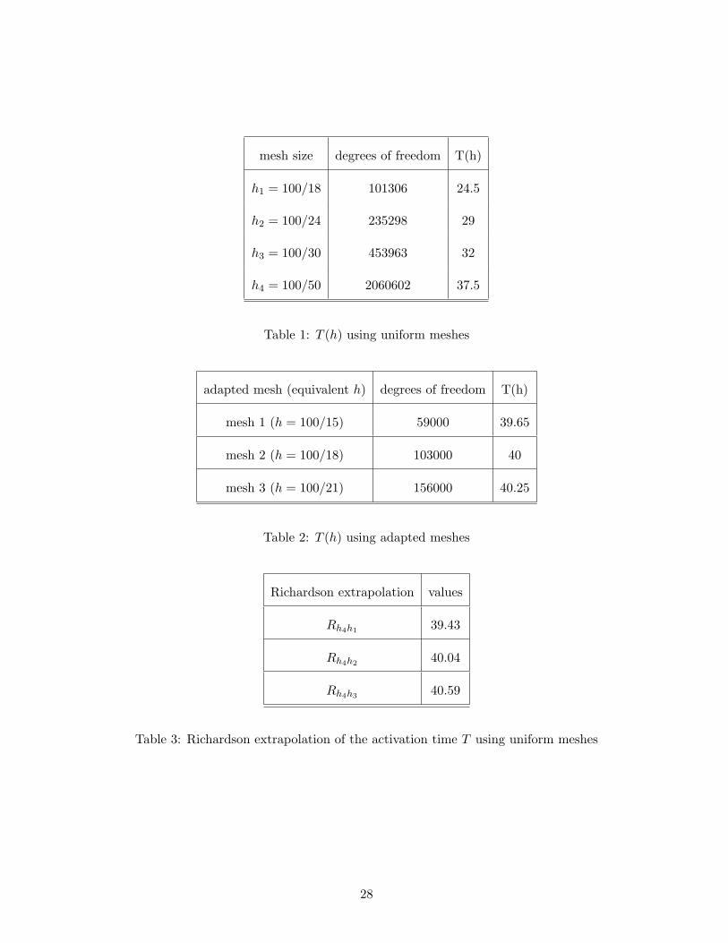
Table 1 shows the approximation T (h) for 4 different uniform meshes. Similarly, Table 2 gives

approximate T (h) for three adapted meshes. The numbers in parenthesis in table 2 are the equivalent

mesh sizes h that would give the same number of degrees of freedom, as if uniform meshes were used

with a quadratic finite element approximation of the solution. These equivalent mesh sizes are given

for comparison. As discussed in the section on the adaptive method, the different adapted meshes were

obtained by varying the target edge length eh, with smaller value of eh leading to finer meshes. The

Richardson extrapolates approximating values of T from the uniform mesh solutions are presented in

table 3. These extrapolates represent a third order approximation for the time T required for the depo-

16

larization front to reach the center of the computational domain. Interestingly enough, the asymptotic

T (h) recovered from Richardson formula are close to the values computed on adapted meshes. This

clearly indicates that the adaptive method gives an accurate value of the depolarisation

time T comparable to the value obtained with Richardson extrapolation. Note that the de-

polarization time is directly connected to the conduction velocity, meaning that the adaptive method

propagates the action potential with the correct wave speed. On the other hand, uniform meshes

are hardly fine enough to properly propagate waves. The coarser is the mesh, the larger

than the exact value is the conduction velocity.. From the depolarization time T (h) in Table 1

and a reference value of T of about 40, we deduce that this conduction velocity is overestimated by

63% and 6.6% on the coarsest and finest uniform meshes, respectively.

Figure 4 presents the solutions U and V at the center of the cube as a function of time obtained

with adapted meshes for different values of the target edge length eh. The adapted solutions correspond

to the test cases in table 2. Not only the depolarisation time T is properly computed with the adap-

tive method, but also the solution is uniformly accurate over time steps and nearly mesh-independent.

The mesh-independence can be seen from the almost perfect superposition of the graphs for the three

adapted solutions shown, in spite of the fact that small meshes with few points are used. Mesh inde-

pendence was not reached for the uniform meshes even with 2060602 dof.

To illustrate the gain in computational time using the adaptive method presented in this work, two

numerical solutions with equal accuracy were obtained, one over a uniform mesh with 2 060 602 dof and

an adapted solution with around 48 000 dof. The equal accuracy was assessed by checking that these

solutions are nearly superposed (see figure 5). The average computational time per time step required

to solve Aliev-Panfilov model using 2 060 602 dof is 820 seconds. However, with the adaptive method,

only 128 seconds are required to obtain similar solution with an average of 48 000 dof. One time step,

17

using the adaptive method, consists in the steps (1) to (5) presented in the section 3. The work load

in the finite element solver is small with the adapted meshes (equivalent to computing a solution on a

coarse uniform mesh with an equivalent mesh size of h = 100/15), but some CPU time is required for

computing the error estimator and generating a new mesh at each time step. Still, simulations take

6.4 times less CPU time with the adaptive method, and the memory requirements are much smaller.

Moreover, as shown above, mesh-independent solutions are achievable with a little extra effort using

the adaptive method (by only bringing the number of dof to 100 000), while this is hardly possible with

uniform meshes.

Finally, the figure 6 illustrates the evolution of the transmembrane potential U and the adapted

mesh. Once again, the front position is well captured and the solution seems uniformly accurate over

time steps.

4.2 Heart geometry

A test problem will now be solved using a realistic heart geometry. The geometry has been obtained

by dissection of a dog’s heart, and the data is available from the Bioengineering Research Group at

the University of Auckland (see Nash [34]). The ventricular myocardium is reproduced, namely the

right and left ventricles. The original geometry was post-processed using the YAMS software to obtain

a surfacic mesh. A volumic mesh was then generated using the GHS3D mesh generator. Details on

the conversion process are given in Sermesant et al. [42]. Finally the volumic mesh was entered in

the MEF++ finite element software, so that anisotropic mesh adaption could be done. Note that

MEF++ [22] has its own internal representation of the heart boundary for the generation/deletion of

mesh points on the surface of the heart. Results will be presented for adapted and uniform meshes.

The mesh used is an unstructured mesh composed of around 71 000 isotropic tetrahedra, “isotropic” in

the sense that the edges of any tetrahedra have nearly equal length and “uniform” meaning that these

18

edge lengths vary mildly across the mesh.

In the rest of this paper, all results are based on the Aliev-Panfilov model with the physical pa-

rameters presented in the previous section. Homogeneous Neumann conditions are imposed on all

boundaries. The initial transmembrane potential and the recovery variable are set to the equilibrium

value U = 0 and V = 0, respectively. An electrical wave is initiated by the current Is given by:

Is =

0.1 if x > 100 and 0 ≤ t ≤ 2,

0 otherwise.

The region x > 100 corresponds to the apex of the heart. The current Is mimicks the electrical wave

coming from the Purkinje network. This current generates a single action potential travelling upward

from the apex towards the base of the heart.

Figure 7 presents the transmembrane potential on the heart boundary at two different times t = 27

and t = 60 t.u., both for the adapted and uniform meshes. The depolarization and repolarization

fronts are smooth and well captured on the adapted anisotropic mesh, in spite of the fact that these

fronts correspond to sharp gradients of the transmembrane potential. The transmembrane potential is

not as clearly represented on the uniform isotropic mesh, even if more than twice the number of dof

are used compared to the adapted solution. On the adapted meshes, the transmembrane potential U

takes values between 0 and 1 while on the uniform mesh, U takes values slightly negative or larger

than 1. The monotonicity of the solution is not guaranteed due to the lack of resolution of the uniform

mesh. As for the test case on the cube, the action potential travels too rapidly on this relatively coarse

uniform mesh, leading to a larger region of depolarized tissue than what is predicted by the adapted

solution. Note that we used the model parameter values published by Aliev and Panfilov [3]) for all our

test cases. We do not pretend that these values properly predict the size of the depolarized region. We

19

only claim that adapted meshes or very fine uniform meshes are required for the conduction velocity

and the size of the activated region to depend only on model parameters and not on the mesh resolution.

Figure 8 shows the adapted meshes again at times t = 27 and t = 60 t.u., both on the heart

surface and on a cross-section of the myocardium. As can be seen, the adapted mesh evolves with time

and, at each time step, elongated elements are obtained at the appropriate position to capture the

transmembrane potential front. An essential ingredient of our mesh adaption method is the addition

and deletion of points on the heart boundary. The action potential is propagated in the interior of the

domain but also on the surface of the heart due to the homogeneous Neumann boundary conditions

used. Points must then be added on the boundary while the wave passes by and deleted once the

wave is gone. The new points must be projected on the heart surface, whose representation must be

independent from any of the time-dependent adapted mesh to guarantee that the heart geometry is

maintained over time steps. The number of tetrahedral elements obtained for these time-dependent

adapted meshes stays around 31000 for all time steps, leading to a nonlinear system of about 96000 dof.

4.3 Heart geometry: presence of pacemaker

A third test case is now presented on the same realistic heart geometry but this time with two waves,

to see how the mesh adaption method works in the presence of interacting waves. A first wave would

be the action potential naturally growing in the LV and the second wave would be generated by a

pacemaker in the RV. The electrical wave in the LV is generate by the following current Is:

Is =

0.1 if

√(x− 82)2 + (y − 23)2 + (z − 92)2 ≤ 5 and 0 ≤ t ≤ 4,

0 otherwise.

20

The wave in the RV comes from the following stimulation current:

Is =

0.1 if x > 100,−0.13x− 0.99y − 0.041z + 99 ≤ 0 and 0 ≤ t ≤ 4,

0 otherwise.

All physical parameters, boundary and initial conditions are the same as in the previous section.

In this problem, the two waves are generated from small stimulated regions near the heart surface that

must be sufficiently refined for the transmembrane potential to grow and start propagating. This would

lead to uniform meshes with about 106 nodes for the whole heart geometry, resulting in excessive CPU

time to simulate a single heart beat. However, the mesh with the adaptive method is refined only in

the vicinity of the pacemaker and the total number of element is greatly reduced.

Figure 9 shows the evolution of the transmembrane potential at three different times with both

adaptive and uniform meshes. Again, the adaptive mesh is crucial to determine an accurate transmem-

brane potential. The adapted meshes also provide a monotone transmembrane potential with values

between 0 and 1, which is not the case with the uniform mesh. Figure 10 show the adapted meshes for

the same times on the surface and on a cross-section of the heart. The interacting waves are properly

represented in the adapted mesh at the bottom of this figure.

5 Conclusions

An accurate numerical method for the transmembrane potential was presented. The accuracy of the

numerical solutions was obtained by using an anisotropic time-dependent adaptive method. This seems

to be a competitive approach for simulations in cardiac electrophysiology compared to the usual uniform

mesh methods commonly used. Results were presented for two ionic models, namely the FitzHugh-

Nagumo and Aliev-Panfilov models. It will be interesting to see how the method performs with more

21

complex ionic models. The performance and the accuracy of the proposed method were illustrated

using a realistic heart geometry, showing the potential for simulations on patient-based geometries.

References

[1] D. Ait Ali Yahia, G. Baruzzi, W. G. Habashi, M. Fortin, J. Dompierre, and M.-G. Val-

let. Anisotropic Mesh Adaptation: Towards User-Independent, Mesh-Independent and Solver-

Independent CFD. Part II: Structured Grids. Int. J. Numer. Meth. Fluids, 39:657–673, 2002.

[2] F. Alauzet, P.L. George, B. Mohammadi, P.J. Frey, and H. Borouchaki. Transient Fixed Point

Based Unstructred Mesh Adaptation. Int. J. Numer. Methods Fluids, 43(6-7):729–745, 2003.

[3] R.R. Aliev and A.V. Panfilov. A Simple Two-Variable Model of Cardiac Excitation. Chaos,

Solitons and Fractals, 7(3):293–301, 1996.

[4] S. Balay, K. Buschelman, V. Eijkhout, W. Gropp, D. Kaushik, M. Knepley, L. C. McInnes,

B. Smith, and H. Zhang. PETSc Users Manual. Technical Report ANL-95/11-Revision 2.1.6,

Argonne National Laboratory, Argonne, Illinois, 2003. http://www.mcs.anl.gov/petsc/.

[5] Y. Belhamadia. A Time-Dependent Adaptive Remeshing for Electrical Waves of the Heart. IEEE

Transactions on Biomedical Engineering, 55(2, Part-1):443–452, 2008.

[6] Y. Belhamadia, A. Fortin, and E. Chamberland. Anisotropic Mesh Adaptation for the Solution

of the Stefan Problem. Journal of Computational Physics, 194(1):233–255, 2004.

[7] Y. Belhamadia, A. Fortin, and E. Chamberland. Three-Dimensional Anisotropic Mesh Adaptation

for Phase Change Problems. Journal of Computational Physics, 201(2):753–770, 2004.

[8] Y. Bourgault, M. Ethier, and V.G. LeBlanc. Simulation of Electrophysiological Waves With an

Unstructured Finite Element Method. Mathematical Modelling and Numerical Analysis, 37(4):649–

662, 2003.

22

[9] E.M. Cherry, H.S. Greenside, and C. S. Henriquez. Efficient Simulation of Three-dimensional

Anisotropic Cardiac Tissue Using an Adaptive Mesh Refinement Method. Chaos: An Interdisci-

plinary Journal of Nonlinear Science, 13(3):853–865, 2003.

[10] P. Colli Franzone, P. Deufhard, B. Erdmann, J. Lang, and L. F. Pavarino. Adaptivity in Space and

Time for Reaction-Diffusion Systems in Electrocardiology. SIAM Journal on Scientific Computing,

28(3):942–962, 2006.

[11] P. Colli Franzone and L. F. Pavarino. A Parallel Solver for Reaction-Diffusion Systems in Compu-

tational Electrocardiology. Math. Models and Methods in Applied Sciences, 14(6):883–911, 2004.

[12] P. Colli Franzone, L. F. Pavarino, and B. Taccardi. Simulating Patterns of Excitation, Repolar-

ization and Action Potential Duration with Cardiac Bidomain and Monodomain Models. Mathe-

matical Biosciences, 197:35–66, 2005.

[13] P. Colli Franzone, L. F. Pavarino, and B. Taccardi. Effects of Transmural Electrical Heterogeneities

and Electrotonic Interactions on the Dispersion of Cardiac Repolarization and Action Potential

Duration: A Simulation Study. Mathematical Biosciences, 204:132–165, 2006.

[14] J. Dompierre, M.-G. Vallet, Y. Bourgault, M.. Fortin, and W. G. Habashi. Anisotropic Mesh

Adaptation: Towards User-Independent, Mesh-Independent and Solver-Independent CFD. Part

III: Unstructured Meshes. Int. J. Numer. Meth. Fluids, 39:675–702, 2002.

[15] V. Elharrar and B. Surawicz. Cycle Length Effect on Restitution of Action Potential Duration in

Dog Cardiac Fibers. Am J Physiol Heart Circ Physiol., 244(6):H782–H792, 1983.

[16] M. Ethier and Y. Bourgault. Semi-implicit time-discretization schemes for the bidomain model.

SIAM Journal of Numerical Analysis, 46(5):2443–2468, 2008.

[17] R.A. FitzHugh. Impulses and Physiological States in Theoretical Models of Nerve Membrane.

Biophys. J, 1:445–466, 1961.

23

[18] A. Fortin and Y. Belhamadia. Numerical Prediction of Freezing Fronts in Cryosurgery: Compar-

ison with Experimental Results. Comput. Methods Biomech. Biomed. Eng., 8(4):241–249, 2005.

[19] A. Fortin and K. Benmoussa. An Adaptive Remeshing Strategy for Free-Surface Fluid Flow

Problems. Part II: the Three-dimensional Case. J. of Polymer Engrg., 26(1):59–86, 2006.

[20] P. Colli Franzone and L. F. Pavarino. A parallel solver for reaction-diffusion systems in compu-

tational electrocardiology. Mathematical Models and Methods in Applied Sciences, 14(6):883–912,

2004.

[21] P.J. Frey and P.L. George. Maillages. Application to Finite Elements. Hermes Science Publishing,

Oxford, 1999.

[22] GIREF. http://www.giref.ulaval.ca/projets/.

[23] W. G. Habashi, J. Dompierre, Y. Bourgault, D. Ait Ali Yahia, M. Fortin, and M.-G. Val-

let. Anisotropic Mesh Adaptation: Towards User-Independent, Mesh-Independent and Solver-

Independent CFD. Part I: General Principles. Int. J. Numer. Meth. Fluids, 32:725–744, 2000.

[24] F. Hecht and B. Mohammadi. Mesh Adaptation by Metric Control for Multi-Scale Phenomena

and Turbulence. AIAA, 97–0859, 1997.

[25] A. L. Hodgkin and A. F. Huxley. A Quantitative Description of Membrane Current and its

Application to Conduction and Excitation in Nerve. Journal of Physiology, 117:500–544, 1952.

[26] N. Hooke, C. S. Henriquez, P. Lanzkron, and D. Rose. Linear algebraic transformations of the

bidomain equations: Implications for numerical methods. Mathematical Biosciences, 120(2):127–

145, 1994.

24

[27] M.G. Karpoukhin, B.Y. Kogan, and J. W. Karplus. The Application of a Massively Parallel

Computer to the Simulation of Electrical Wave Propagation Phenomena in the Heart Muscle

Using Simplified Models. HICSS, 5:112–122, 1995.

[28] J. P. Keener and K. Bogar. A numerical method for the solution of the bidomain equations in

cardiac tissue. Chaos, 8:234–241, 1998.

[29] G.T. Lines, M.L. Buist, P. Grottum, A.J. Pullan, J. Sundnes, and A. Tveito. Mathematical models

and numerical methods for the forward problem in cardiac electrophysiology. Comput. Visual. Sc.,

5:215–239, 2003.

[30] G.T. Lines, P. Grottum, and A. Tveito. Modeling the electrical activity of the heart: A bidomain

model of the ventricles embedded in a torso. Comput. Visual. Sc., 5:195–213, 2003.

[31] C. Manole, M.-G. Vallet, J. Dompierre, and F. Guibault. Benchmarking Second Order Derivatives

Recovery of a Piecewise Linear Scalar Field. Proceedings of the 17th IMACS World Congress

Scientific Computation, Applied Mathematics and Simulation, 2005.

[32] M. Murillo and X.C. Cai. A fully implicit parallel algorithm for simulating the non-linear electrical

activity of the heart. Numerical Linear Algebra with Applications, 11:261–277, 2004.

[33] J. S. Nagumo, S. Arimoto, and S. Yoshizawa. An Active Pulse Transmission Line Simulating

Nerve Axon. Proc IRE, 50:2061–2071, 1962.

[34] M. Nash. Mechanics and Material Properties of the Heart using an Anatomically Accurate Math-

ematical Model. PhD thesis, University of Auckland, New Zealand, 1998.

[35] M.P. Nash and A.V. Panfilov. Electromechanical Model of Excitable Tissue to Study Reentrant

Cardiac Arrhythmias. Progress in Biophysics & Molecular Biology, 85:501–522, 2004.

25

[36] A.V. Panfilov, A.V.and Holden, editor. Computational Biology of the Heart. John Wiley & Sons,

1997.

[37] R.C. Penland, D.M. Harrild, and C.S. Henriquez. Modeling impulse propagation and extracellular

potential distribution in anisotropic cardiac tissue using a finite volume element discretization.

Comput. Visual. Sc., 4:215–226, 2002.

[38] M. Pennacchio and V. Simoncini. Efficient algebraic solution of reaction-diffusion systems for the

cardiac excitation process. Journal of Computational and Applied Mathematics, 145:49–70, 2002.

[39] B. J. Roth. Approximate Analytical Solutions to the Bidomain Equations with Unequal Anisotropy

Ration. Physical Review E, 55:1819–1826, 1997.

[40] B.J. Roth. Meandering of spiral waves in anisotropic cardiac tissue. Physica D, 150:127–136, 2001.

[41] Y. Saad. Iterative Methods for Sparse Linear Systems. PWS Publishing Company, 1996.

[42] M. Sermesant, Y. Coudiere, H. Delingette, N. Ayache, and J. A. Desideri. An electro-mechanical

model of the heart for cardiac image analysis. In W. J. Niessen and M. A. Viergever, editors,

Medical Image Computing And Computer-Assisted Intervention - MICCAI 2001. 4th International

Conference, number 2208 in Lect. Notes Comput. Sci., pages 224–231. Springer, 2001.

[43] J. Sundnes. Numerical Methods for Simulating the Electrical Activity of the Heart. PhD thesis,

University of Oslo, 2002.

[44] J. Sundnes, G. Lines, and A. Tveito. An Operator Splitting Method for Solving the Bido-

main Equations Coupled to a Volume Conductor Model for the Torso. Mathematical biosciences,

194(2):233–248, 2005.

[45] J.A. Trangenstein and C. Kim. Operator Splitting and Adaptive Mesh Refinement for the Luo-

Rudy I Model. Journal of Computational Physics, 196(2):645–679, 2004.

26

[46] M. L. Trew, B. H. Smaill, D. P. Bullivant, P. J. Hunter, and A. J. Pullan. A Generalized Finite Dif-

ference Method for Modeling Cardiac Electrical Activation on Arbitrary, Irregular Computational

Meshes. Mathematical Biosciences, 198(2):169–189, 2005.

[47] E. J. Vigmond, F. Aguel, and N. A. Trayanova. Computational Techniques for Solving the Bido-

main Equations in Three Dimensions. IEEE Trans. Biomed. Eng., 49(11):1260–9, 2002.

[48] R. Weber Dos Santos, G. Plank, S. Bauer, and E.J. Vigmond. Preconditioning techniques for the

bidomain equations. In Proceedings of the 15th International Conference on Domain Decomposi-

tion Methods, pages 571–580. Springer, Lecture Notes in Computational Science and Engineering

(LNCSE)., 2003.

[49] R. Weber dos Santos, G. Plank, S. Bauer, and E.J. Vigmond. Parallel Multigrid Preconditioner

for the Cardiac Bidomain Model. IEEE Trans. Biomed. Eng., 51(11):1960–1968, 2004.

[50] W. Ying. A Multilevel Adaptive Approach for Computational Cardiology. PhD thesis, Duke

University, Durham, USA, 2005.

27

mesh size degrees of freedom T(h)

h1 = 100/18 101306 24.5

h2 = 100/24 235298 29

h3 = 100/30 453963 32

h4 = 100/50 2060602 37.5

Table 1: T (h) using uniform meshes

adapted mesh (equivalent h) degrees of freedom T(h)

mesh 1 (h = 100/15) 59000 39.65

mesh 2 (h = 100/18) 103000 40

mesh 3 (h = 100/21) 156000 40.25

Table 2: T (h) using adapted meshes

Richardson extrapolation values

Rh4h1 39.43

Rh4h2 40.04

Rh4h3 40.59

Table 3: Richardson extrapolation of the activation time T using uniform meshes

28

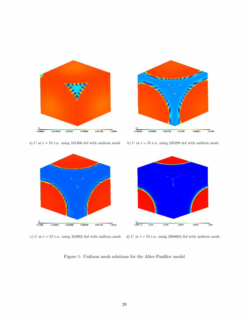
a) U at t = 55 t.u. using 101306 dof with uniform mesh b) U at t = 55 t.u. using 235298 dof with uniform mesh

c) U at t = 55 t.u. using 453962 dof with uniform mesh d) U at t = 55 t.u. using 2060602 dof with uniform mesh

Figure 1: Uniform mesh solutions for the Aliev-Panfilov model

29

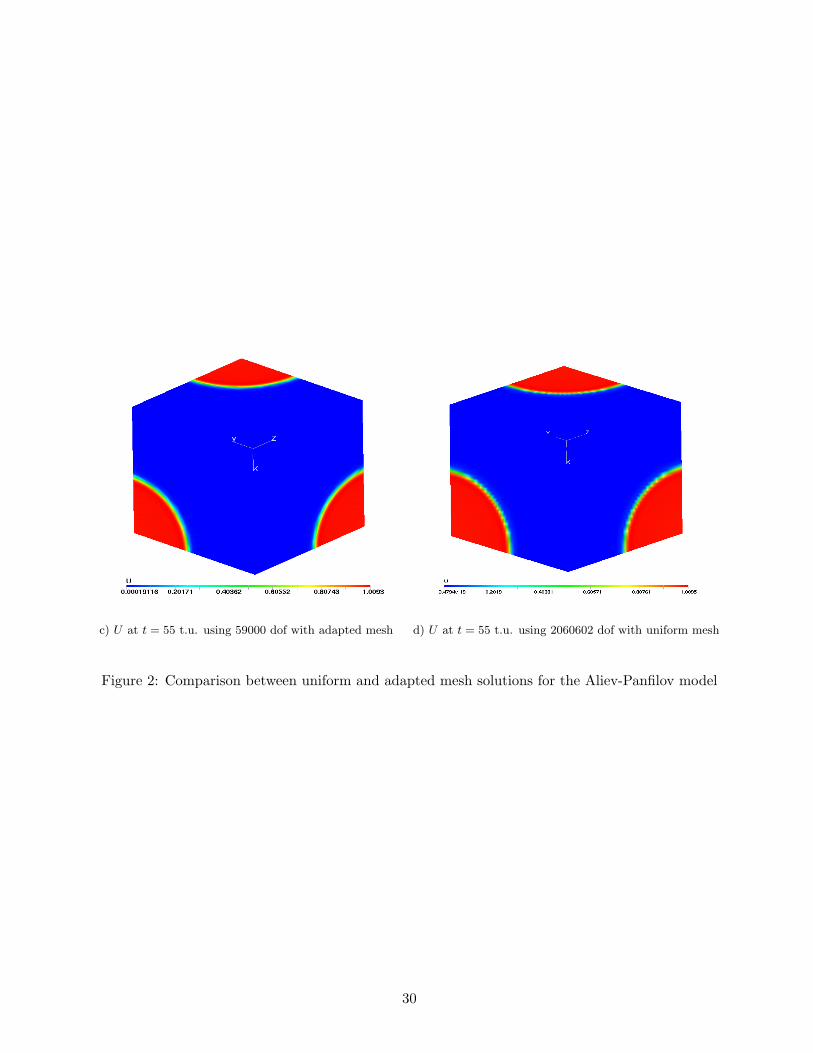
c) U at t = 55 t.u. using 59000 dof with adapted mesh d) U at t = 55 t.u. using 2060602 dof with uniform mesh

Figure 2: Comparison between uniform and adapted mesh solutions for the Aliev-Panfilov model

30

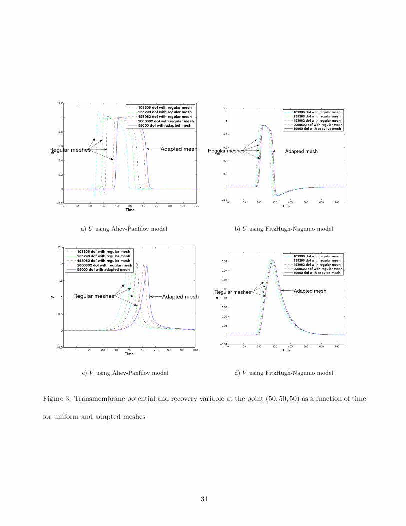
a) U using Aliev-Panfilov model b) U using FitzHugh-Nagumo model

c) V using Aliev-Panfilov model d) V using FitzHugh-Nagumo model

Figure 3: Transmembrane potential and recovery variable at the point (50, 50, 50) as a function of time

for uniform and adapted meshes

31

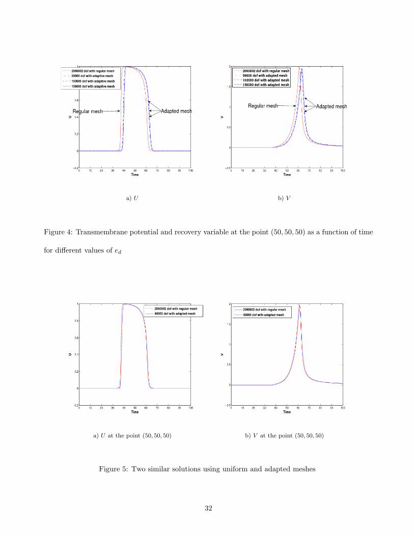
a) U b) V

Figure 4: Transmembrane potential and recovery variable at the point (50, 50, 50) as a function of time

for different values of ed

a) U at the point (50, 50, 50) b) V at the point (50, 50, 50)

Figure 5: Two similar solutions using uniform and adapted meshes

32

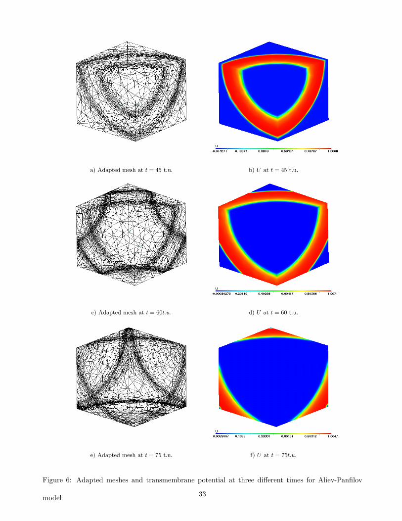
a) Adapted mesh at t = 45 t.u. b) U at t = 45 t.u.

c) Adapted mesh at t = 60t.u. d) U at t = 60 t.u.

e) Adapted mesh at t = 75 t.u. f) U at t = 75t.u.

Figure 6: Adapted meshes and transmembrane potential at three different times for Aliev-Panfilov

model 33

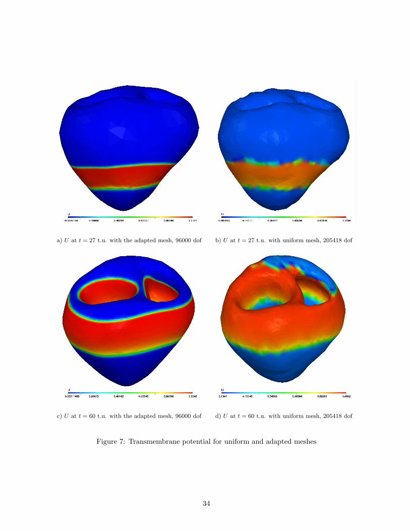
a) U at t = 27 t.u. with the adapted mesh, 96000 dof b) U at t = 27 t.u. with uniform mesh, 205418 dof

c) U at t = 60 t.u. with the adapted mesh, 96000 dof d) U at t = 60 t.u. with uniform mesh, 205418 dof

Figure 7: Transmembrane potential for uniform and adapted meshes

34

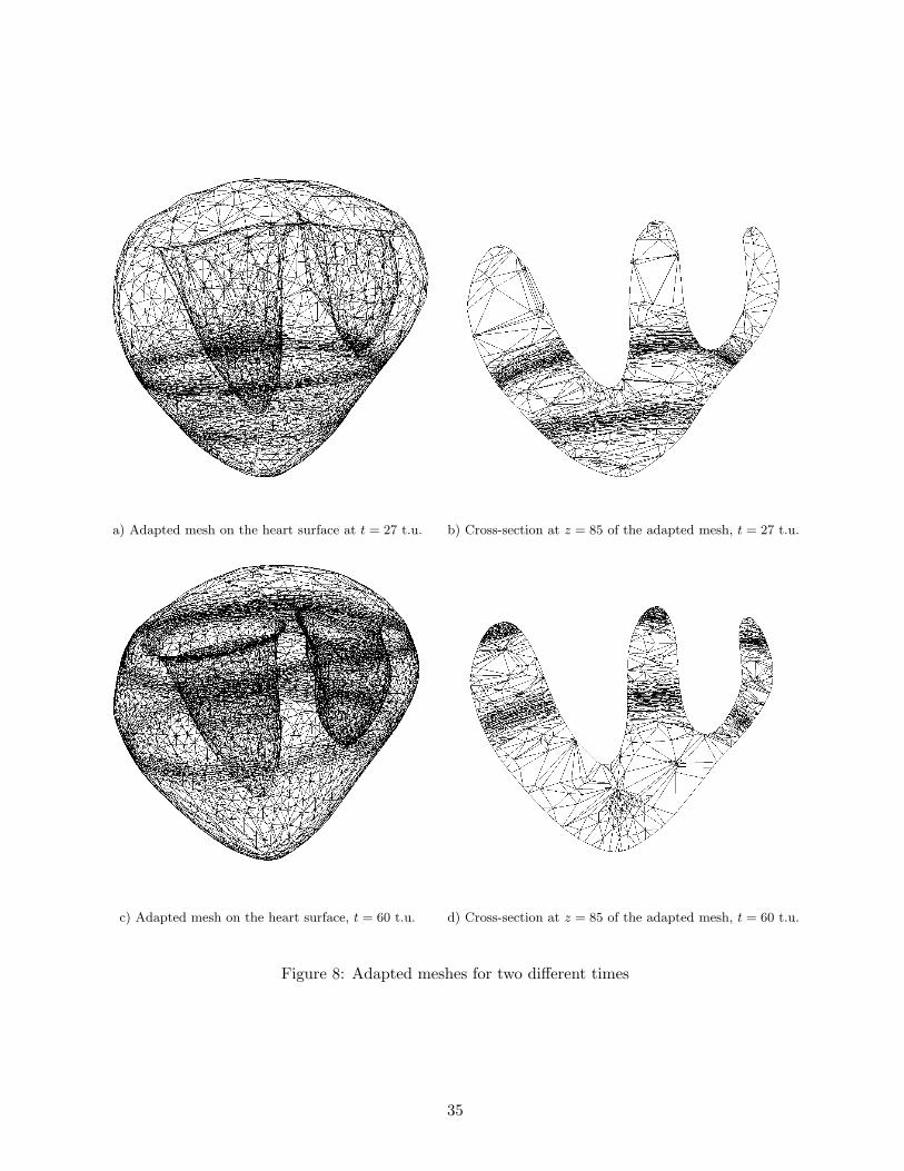
a) Adapted mesh on the heart surface at t = 27 t.u. b) Cross-section at z = 85 of the adapted mesh, t = 27 t.u.

c) Adapted mesh on the heart surface, t = 60 t.u. d) Cross-section at z = 85 of the adapted mesh, t = 60 t.u.

Figure 8: Adapted meshes for two different times

35

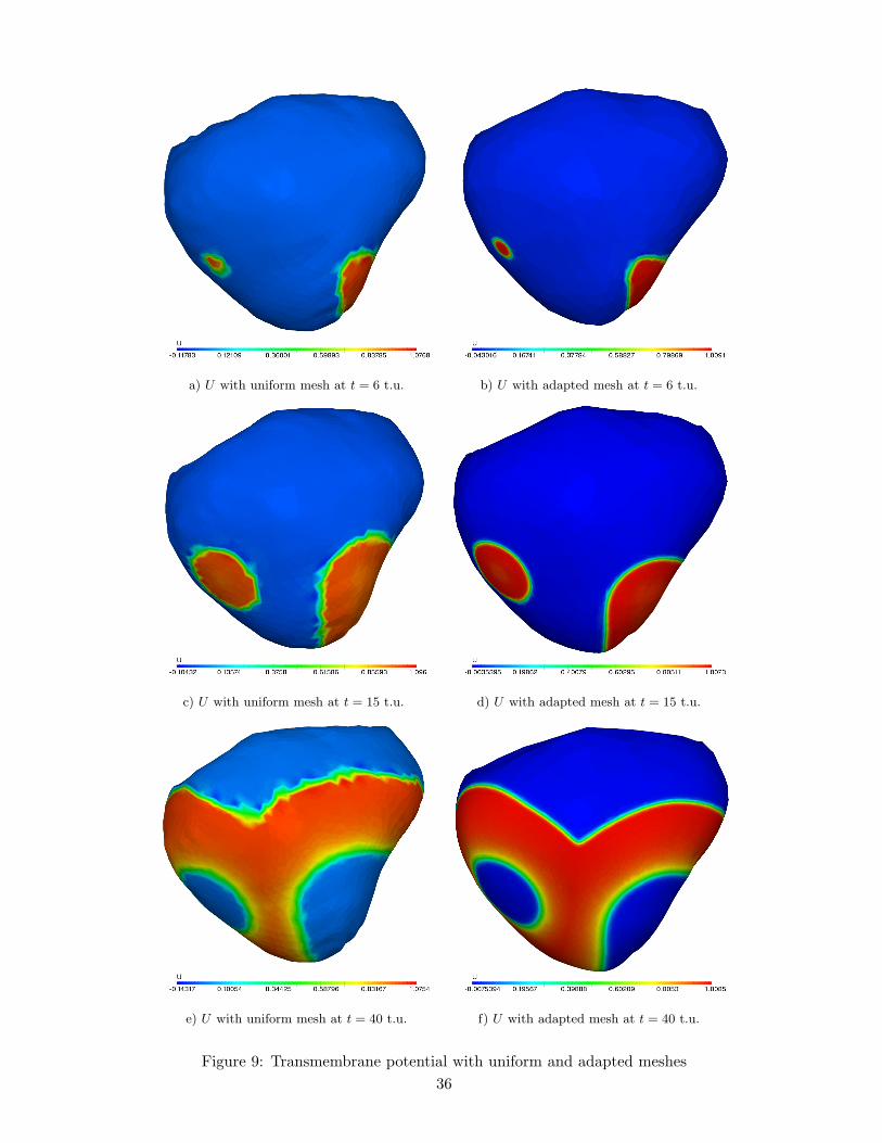
a) U with uniform mesh at t = 6 t.u. b) U with adapted mesh at t = 6 t.u.

c) U with uniform mesh at t = 15 t.u. d) U with adapted mesh at t = 15 t.u.

e) U with uniform mesh at t = 40 t.u. f) U with adapted mesh at t = 40 t.u.

Figure 9: Transmembrane potential with uniform and adapted meshes36

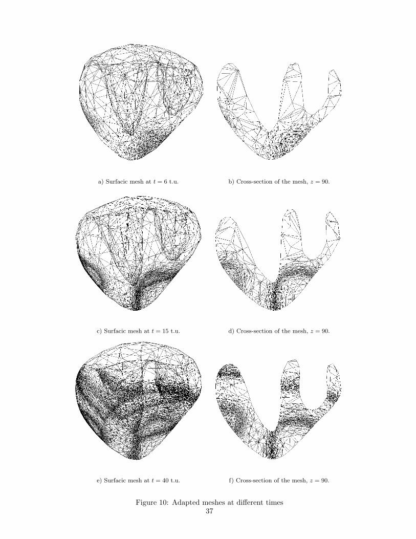
a) Surfacic mesh at t = 6 t.u. b) Cross-section of the mesh, z = 90.

c) Surfacic mesh at t = 15 t.u. d) Cross-section of the mesh, z = 90.

e) Surfacic mesh at t = 40 t.u. f) Cross-section of the mesh, z = 90.

Figure 10: Adapted meshes at different times37