
Towards a practical parallelisation of the revised simplex ... · Overview LP problems and the...
57
Towards a practical parallelisation of the revised simplex method Julian Hall, Edmund Smith and Huangfu Qi School of Mathematics University of Edinburgh 14th September 2010 Towards a practical parallelisation of the revised simplex method
Transcript of Towards a practical parallelisation of the revised simplex ... · Overview LP problems and the...

Towards a practical parallelisation of therevised simplex method
Julian Hall, Edmund Smith and Huangfu Qi
School of Mathematics
University of Edinburgh
14th September 2010
Towards a practical parallelisation of the revised simplex method

Overview
• LP problems and the simplex method
• Scope parallelism
• (Preliminary) results
• Conclusions
Towards a practical parallelisation of the revised simplex method1

Linear programming (LP) and the simplex method
minimize f = cTx
subject to Ax = b x ≥ 0

Linear programming (LP) and the simplex method
minimize f = cTx
subject to Ax = b x ≥ 0
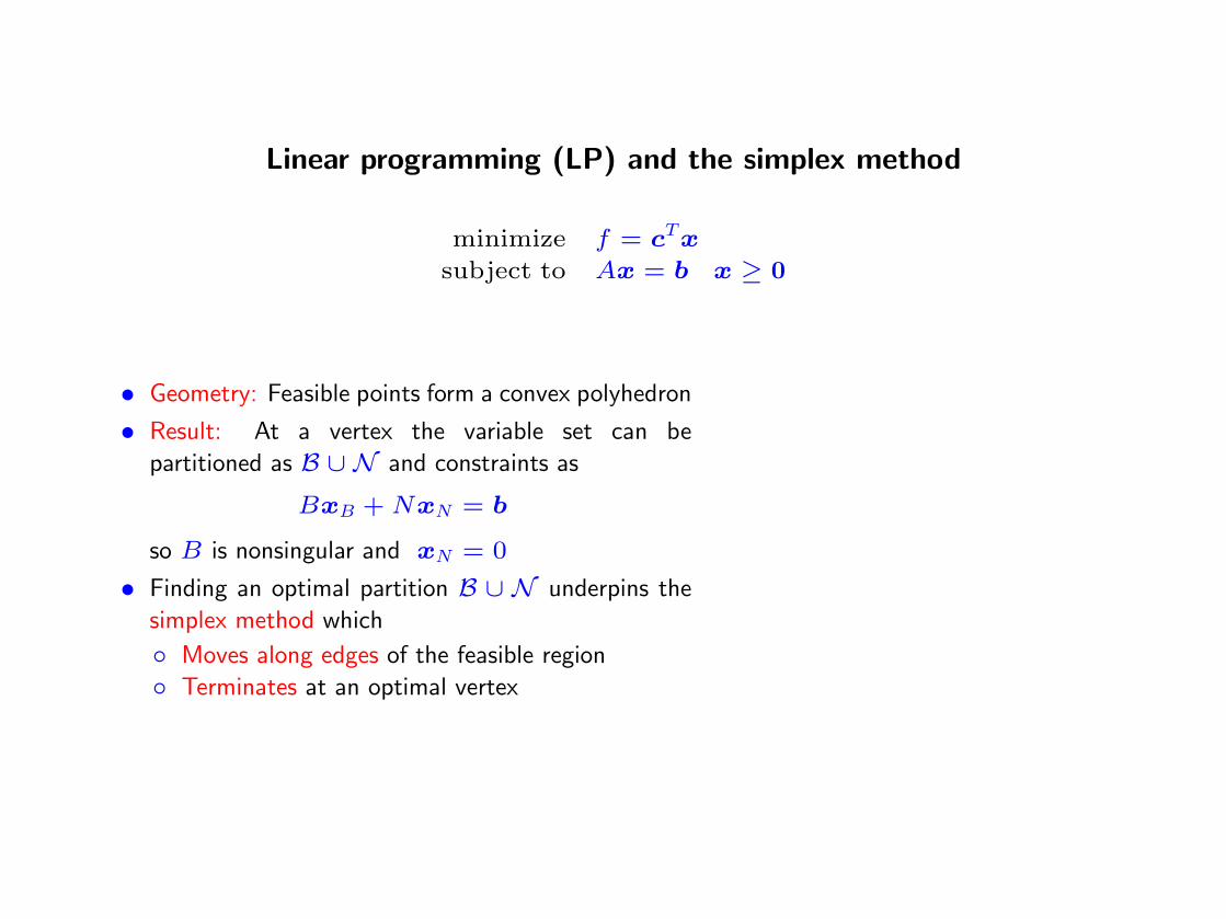
• Geometry: Feasible points form a convex polyhedron

Linear programming (LP) and the simplex method
minimize f = cTx
subject to Ax = b x ≥ 0
• Geometry: Feasible points form a convex polyhedron
• Result: At a vertex the variable set can be
partitioned as B ∪ N and constraints as
BxB +NxN = b
so B is nonsingular and xN = 0

Linear programming (LP) and the simplex method
minimize f = cTx
subject to Ax = b x ≥ 0
• Geometry: Feasible points form a convex polyhedron
• Result: At a vertex the variable set can be
partitioned as B ∪ N and constraints as
BxB +NxN = b
so B is nonsingular and xN = 0
• Finding an optimal partition B ∪ N underpins the
simplex method
Linear programming (LP) and the simplex method
minimize f = cTx
subject to Ax = b x ≥ 0
• Geometry: Feasible points form a convex polyhedron
• Result: At a vertex the variable set can be
partitioned as B ∪ N and constraints as
BxB +NxN = b
so B is nonsingular and xN = 0
• Finding an optimal partition B ∪ N underpins the
simplex method which
◦ Moves along edges of the feasible region
◦ Terminates at an optimal vertex
◦ Has transformed decision making since 1947A is usually sparse
Towards a practical parallelisation of the revised simplex method2

The reduced LP problem
At a vertex, for a partition B ∪ N with B nonsingular, the original problem is
minimize f = cTNxN + cTBxB
subject to N xN + B xB = b
xN ≥ 0 xB ≥ 0.

The reduced LP problem
At a vertex, for a partition B ∪ N with B nonsingular, the original problem is
minimize f = cTNxN + cTBxB
subject to N xN + B xB = b
xN ≥ 0 xB ≥ 0.
Eliminate xB from the objective to give the reduced LP problem
minimize f = sTNxN + f
subject to N xN + I xB = b
xN ≥ 0 xB ≥ 0,
where b = B−1b, N = B−1N and sN is given by
sTN = c
TN − c
TBN
Vertex is optimal ⇐⇒ sN ≥ 0
Towards a practical parallelisation of the revised simplex method3

Implementation: standard simplex method
N B RHS
1... N I b
m
0 sTN 0T −f
In each iteration:
• Choose variable xq with sq < 0 to increase from zero
• Use the pivotal column q of N and b to find the pivotal row p with α = bp/apq
• Exchange indices p and q between B and N• Update tableau corresponding to this basis change
N := N − (1/apq)aqaTp b := b− αaq
sTN := sTN − (sq/apq)aqaTp −f := −f − αsq
Towards a practical parallelisation of the revised simplex method4

Implementation: revised simplex method
• Maintains a representation of B−1 (rather than N)
• Pivotal column is
aq = B−1aq, where aq is column q of A

Implementation: revised simplex method
• Maintains a representation of B−1 (rather than N)
• Pivotal column is
aq = B−1aq, where aq is column q of A
• Pivotal row is
aTp = πTpN , where πTp = eTpB−1

Implementation: revised simplex method
• Maintains a representation of B−1 (rather than N)
• Pivotal column is
aq = B−1aq, where aq is column q of A
• Pivotal row is
aTp = πTpN , where πTp = eTpB−1
• Representation of B−1 is updated by exploiting
B−1
:=
(I −
(aq − ep)eTpapq
)B−1
• Periodically B−1 is formed from scratch
• Efficient solution of large sparse LP problems requires the revised simplex method
Towards a practical parallelisation of the revised simplex method5

Implementation: hyper-sparsity
• Major computational cost each iteration is
forming B−1rF , rTBB−1 and rTπN
• Vectors rF , rB are always sparse
• Vector rπ may be sparse
Implementation: hyper-sparsity
• Major computational cost each iteration is
forming B−1rF , rTBB−1 and rTπN
• Vectors rF , rB are always sparse
• Vector rπ may be sparse
• If the results of these operations are (usually)
sparse then LP is said to be hyper-sparse

Implementation: hyper-sparsity
• Major computational cost each iteration is
forming B−1rF , rTBB−1 and rTπN
• Vectors rF , rB are always sparse
• Vector rπ may be sparse
• If the results of these operations are (usually)
sparse then LP is said to be hyper-sparse
• LP structure means B−1 is sparse

Implementation: hyper-sparsity
• Major computational cost each iteration is
forming B−1rF , rTBB−1 and rTπN
• Vectors rF , rB are always sparse
• Vector rπ may be sparse
• If the results of these operations are (usually)
sparse then LP is said to be hyper-sparse
• LP structure means B−1 is sparse
• Simplex method typically better than interior
point methods for hyper-sparse LP problems
(◦) but frequently not for other LPs (•)
H and McKinnon (1998–2005)
Simplex 10 times faster
2 3 4 5 6
1
2
0
2
1
IPM 10 times faster
log
(IPM
/sim
plex
tim
e)
log (Basis dimension)10
10
IPM 2 times faster
Simplex 2 times faster
Towards a practical parallelisation of the revised simplex method6
Implementation: inverting B
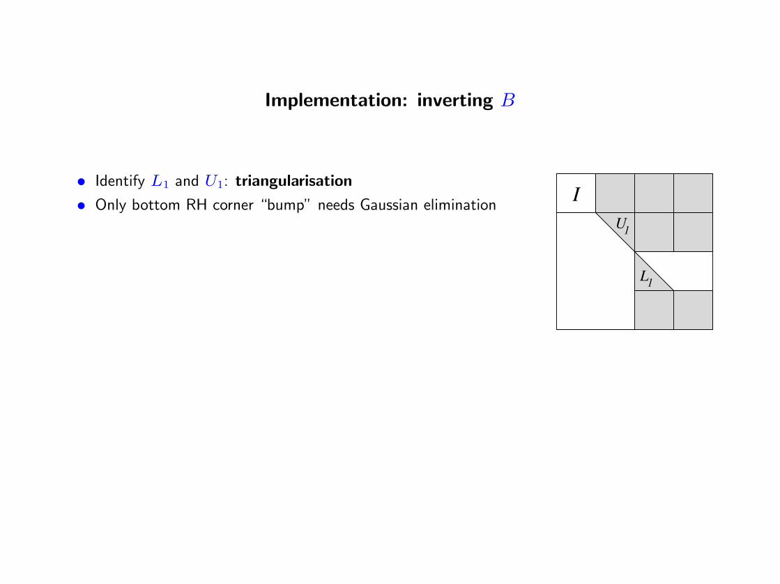
• Identify L1 and U1: triangularisation
• Only bottom RH corner “bump” needs Gaussian eliminationI
1L
1U

Implementation: inverting B
• Identify L1 and U1: triangularisation
• Only bottom RH corner “bump” needs Gaussian eliminationI
1L
1U• For many (hyper-sparse) LP problems, B is highly reducible
◦ Bump is very small
◦ Cost of triangularisation dominates factorization of bump

Implementation: inverting B
• Identify L1 and U1: triangularisation
• Only bottom RH corner “bump” needs Gaussian eliminationI
1L
1U• For many (hyper-sparse) LP problems, B is highly reducible
◦ Bump is very small
◦ Cost of triangularisation dominates factorization of bump
• For other LP problems, factorization dominates triangularisation
• Fill-in when representing B−1 is generally small
◦ Typically < 10%
◦ Sometimes 100%
◦ Rarely > 1000%
Towards a practical parallelisation of the revised simplex method7

Why try to exploit parallelism?

Why try to exploit parallelism?
• Moore’s law drives core counts per processor, but clock speeds will stabilise

Why try to exploit parallelism?
• Moore’s law drives core counts per processor, but clock speeds will stabilise
• Serial performance of simplex is spectacularly good
◦ Flop count per iteration is near optimal
◦ Number of iterations is near optimal
Why try to exploit parallelism?
• Moore’s law drives core counts per processor, but clock speeds will stabilise
• Serial performance of simplex is spectacularly good
◦ Flop count per iteration is near optimal
◦ Number of iterations is near optimal
• Can’t wait for faster serial processors or algorithmic improvement
• Simplex method must try to exploit parallelism
Towards a practical parallelisation of the revised simplex method8
Conventional wisdom: Parallelism
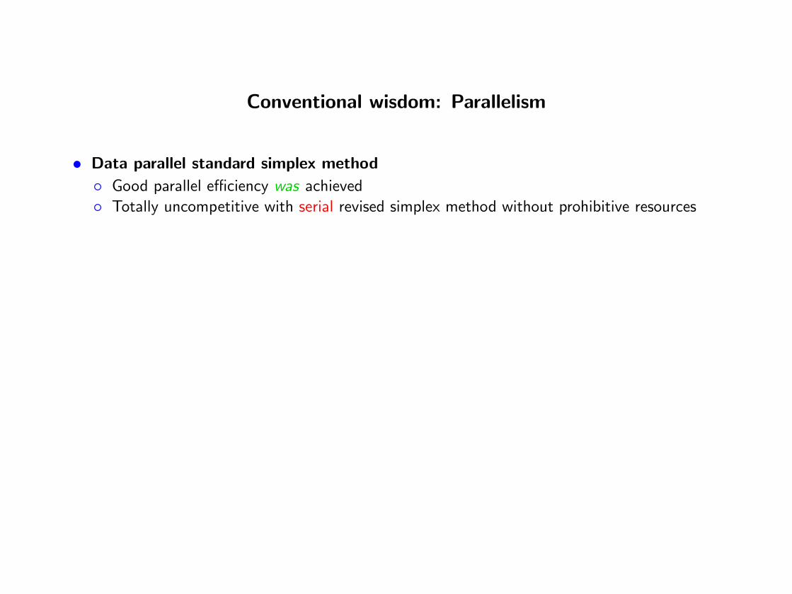
• Data parallel standard simplex method
◦ Good parallel efficiency was achieved
◦ Totally uncompetitive with serial revised simplex method without prohibitive resources

Conventional wisdom: Parallelism
• Data parallel standard simplex method
◦ Good parallel efficiency was achieved
◦ Totally uncompetitive with serial revised simplex method without prohibitive resources
• Data parallel revised simplex method
◦ Only immediate parallelism is in forming rTπN
◦ When n� m, cost of rTπN dominates: significant speed-up was achieved
Bixby and Martin (2000)
• Task parallel revised simplex method
◦ Overlap computational components for different iterations
Wunderling (1996), H and McKinnon (1995-2005)
◦ Modest speed-up was achieved on general sparse LP problems
• All data and task parallel implementations compromised by serial inversion of B
Review: H (2010)
Towards a practical parallelisation of the revised simplex method9

CPU or GPU or both?
Heterogeneous desk-top architectures
CPU:
• Fewer, faster cores
• Relatively slow memory transfer
• Welcomes algorithmically complex code
• Full range of development tools

CPU or GPU or both?
Heterogeneous desk-top architectures
CPU:
• Fewer, faster cores
• Relatively slow memory transfer
• Welcomes algorithmically complex code
• Full range of development tools
GPU:
• More, slower cores
• Relatively fast memory transfer
• Global communication is expensive/difficult
• Very limited development tools
CPU and GPU:
• Answer may be to combine CPU and GPU
Towards a practical parallelisation of the revised simplex method10

Computation and Data
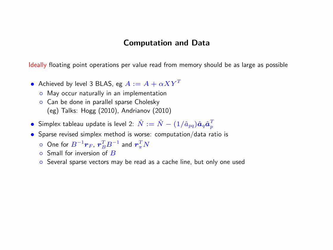
Ideally floating point operations per value read from memory should be as large as possible

Computation and Data
Ideally floating point operations per value read from memory should be as large as possible
• Achieved by level 3 BLAS, eg A := A+ αXY T
◦ May occur naturally in an implementation
◦ Can be done in parallel sparse Cholesky
(eg) Talks: Hogg (2010), Andrianov (2010)

Computation and Data
Ideally floating point operations per value read from memory should be as large as possible
• Achieved by level 3 BLAS, eg A := A+ αXY T
◦ May occur naturally in an implementation
◦ Can be done in parallel sparse Cholesky
(eg) Talks: Hogg (2010), Andrianov (2010)
• Simplex tableau update is level 2: N := N − (1/apq)aqaTp
• Sparse revised simplex method is worse: computation/data ratio is
◦ One for B−1rF , rTBB−1 and rTπN
◦ Small for inversion of B
◦ Several sparse vectors may be read as a cache line, but only one used
• Doesn’t look good
Towards a practical parallelisation of the revised simplex method11
Modified revised simplex method
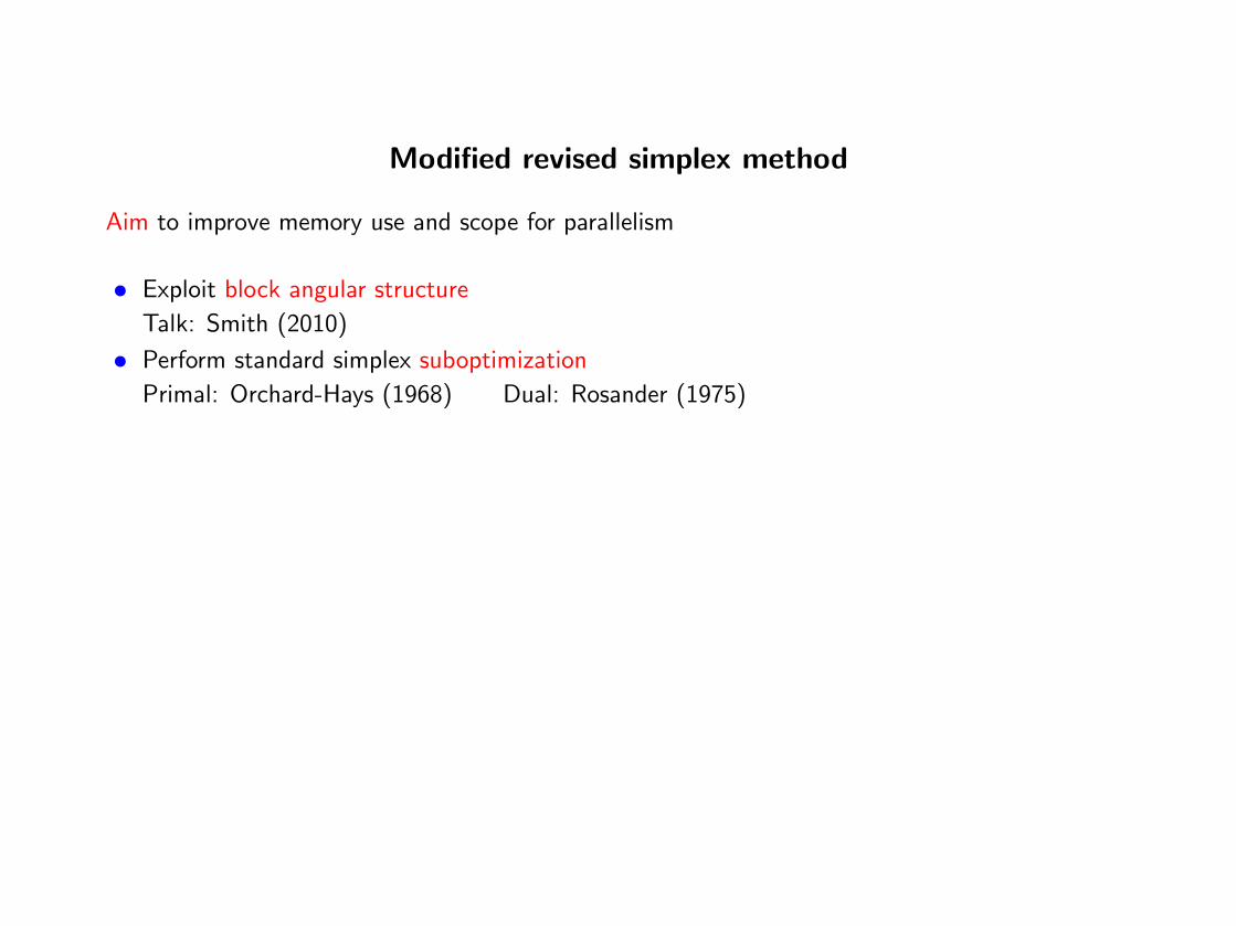
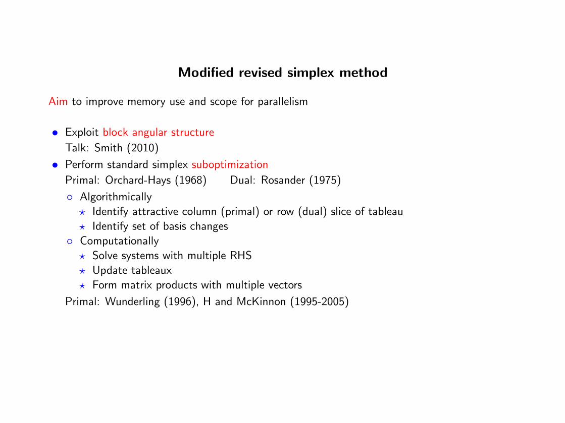
Aim to improve memory use and scope for parallelism

Modified revised simplex method
Aim to improve memory use and scope for parallelism
• Exploit block angular structure
Talk: Smith (2010)
Modified revised simplex method
Aim to improve memory use and scope for parallelism
• Exploit block angular structure
Talk: Smith (2010)
• Perform standard simplex suboptimization
Primal: Orchard-Hays (1968) Dual: Rosander (1975)

Modified revised simplex method
Aim to improve memory use and scope for parallelism
• Exploit block angular structure
Talk: Smith (2010)
• Perform standard simplex suboptimization
Primal: Orchard-Hays (1968) Dual: Rosander (1975)
◦ Algorithmically
? Identify attractive column (primal) or row (dual) slice of tableau
? Identify set of basis changes
◦ Computationally
? Solve systems with multiple RHS
? Update tableaux
? Form matrix products with multiple vectors
Primal: Wunderling (1996), H and McKinnon (1995-2005)
• Perform parallel triangularisation of B
Talk: H (2005)
Towards a practical parallelisation of the revised simplex method12

Other relevant work
• Sparse matrix-vector product Ar
◦ GPU out-performs comparable CPU for full r
(eg) Vuduc et al. (2010)
◦ Revised simplex NTr has sparse r

Other relevant work
• Sparse matrix-vector product Ar
◦ GPU out-performs comparable CPU for full r
(eg) Vuduc et al. (2010)
◦ Revised simplex NTr has sparse r
• Solve A−1r with given A−1 and full r
◦ CPU performance is memory bound
◦ Speed-up factor limited to number of CPUs
(eg) Hogg et al. (2010)
◦ Revised simplex B−1r, rTB−1 have sparse r
Towards a practical parallelisation of the revised simplex method13

Dual revised simplex method with suboptimization
• Computational scheme
◦ On CPU
? Choose attractive row set P? Form πTP = ePB
−1

Dual revised simplex method with suboptimization
• Computational scheme
◦ On CPU
? Choose attractive row set P? Form πTP = ePB
−1
◦ On GPU
? Form aTP = πTPN
? Perform dual standard simplex iterations on aTP to identify column set Q

Dual revised simplex method with suboptimization
• Computational scheme
◦ On CPU
? Choose attractive row set P? Form πTP = ePB
−1
◦ On GPU
? Form aTP = πTPN
? Perform dual standard simplex iterations on aTP to identify column set Q◦ On CPU
? Form aQ = B−1aQ? Invert B

Dual revised simplex method with suboptimization
• Computational scheme
◦ On CPU
? Choose attractive row set P? Form πTP = ePB
−1
◦ On GPU
? Form aTP = πTPN
? Perform dual standard simplex iterations on aTP to identify column set Q◦ On CPU
? Form aQ = B−1aQ? Invert B
◦ Aim to overlap CPU and GPU computation, and with CPU↔ GPU communication
• Yet to be implemented
• Will make use of new ideas for serial dual revised simplex
Towards a practical parallelisation of the revised simplex method14

Standard simplex method on a GPU
• Implemented by Smith as i8

Standard simplex method on a GPU
• Implemented by Smith as i8
• Experiments on machine with two quad-core AMD CPUs and GTX285 NVIDIA GPU
• For dense LP problems, best in red
Solver Type HPC Time Iterations Speed (ms/iter)
gurobi primal serial 1357 16034 84.6
gurobi dual serial 976 14518 67.2
i7 primal serial 6093 44384 137.3
i6 primal SSM parallel 4039 288419 14.0
i8 primal SSM GPU 800 221157 3.6
• Not (really) of practical value but a good learning exercise
• No hope of beating serial solvers on sparse LP problems
Towards a practical parallelisation of the revised simplex method15

Conclusions
• Identified need for simplex method to exploit parallelism
• Identified memory access as severe limitation
◦ Worse with efficient simplex implementation
◦ Worse with modern architectures
• Suggested approaches to improve memory use
• Shown that the standard simplex method will run fast on a GPU
Towards a practical parallelisation of the revised simplex method16