
Towards 24-7 Brain Mapping Technologyetd.dtu.dk/thesis/240392/ep09_17.pdf · Towards 24-7 brain...
71
Towards 24-7 Brain Mapping Technology Brian Nielsen Master’s thesis, March 2009
Transcript of Towards 24-7 Brain Mapping Technologyetd.dtu.dk/thesis/240392/ep09_17.pdf · Towards 24-7 brain...

Towards 24-7 Brain Mapping Technology
Brian Nielsen
Master’s thesis, March 2009

Towards 24-7 Brain Mapping
This master’s thesis is written by: Brian Nielsen, s974663 Supervisor: Professor Lars Kai Hansen
DTU Informatics Intelligent Signal Processing Technical University of Denmark Richard Petersens Plads Building 321 2800 Kgs. Lyngby Denmark www.imm.dtu.dk Phone: (+45) 45 25 33 51 Email: [email protected]
Date of publication:
18 March 2009
Edition:
1. edition
This master’s thesis serves as documentation for the final assignment in the requirements to achieve the degree Master of Science in Engineering. The report represents 30 ECTS points.
© Brian Nielsen, 2009
The front page illustration shows a computer simulation of pyramidal cells in the neocortex (Markram, 2009).
Towards 24-7 brain mapping technology DTU, March 2009
I
Abstract The use of closely spaced subcutaneously implanted electrodes for EEG recording is
examined.
A comparison between conventional electrodes and subcutaneous electrodes is made.
Only a limited amount of data material is available. Several methods are employed for
the comparison: frequency spectra, ERP, the amount of artifacts, and ICA
decomposition. The analysis shows that the data recorded from the two different
recording methods is almost identical, although some differences are found. The found
differences do not give a clear picture of whether the subcutaneous electrodes provide
better or worse data compared to the conventional electrodes.
A classification of two different data sets is done in order to investigate the use of a
limited amount of electrodes: 1) Classification of a data set containing visual evoked
potential (VEP) trials is performed by three different classification methods: Fisher’s
linear discriminant (FLD), linear support vector machines (SVM), and Gaussian SVM. A
good classification from the supplied data is not possible. 2) Classification of a data set
containing tasks based on motor imagery is performed. FLD, linear SVM, and Gaussian
SVM are used as classifiers. Feature extraction is performed on the basis of event
related potential (ERP) and event related spectral perturbation (ERSP). Using only four
electrodes a classification accuracy of 94% is obtained. The results from the second
classification show that it is possible to perform a successful classification using only a
few electrodes.

Towards 24-7 brain mapping technology DTU, March 2009
II
Preface This master’s thesis has been carried out in the time from 25 August 2008 to 18 March
2009 at the Intelligent Signal Processing group at DTU Informatics institute, Technical
University of Denmark. The work has been supervised by Professor Lars Kai Hansen. I
would like to thank him for the inspiration and guidance he provided. I would also like to
thank the people at Hypo-Safe A/S who also offered inspiration and willingly provided
part of the data which is used in this project.
Kgs. Lyngby, 18 March 2009
Brian Nielsen, s974663

Towards 24-7 brain mapping technology DTU, March 2009
III
Contents 1 Introduction ....................................................................................................... 1
1.1 Problem description ............................................................................................ 3
1.2 Guide to this report ............................................................................................. 4
2 The brain and EEG .............................................................................................. 5
2.1 Structure of the brain .......................................................................................... 5
2.2 Dipoles ................................................................................................................. 7
2.3 Brain current sources ........................................................................................ 10
2.4 From current sources to scalp potential ............................................................ 12
2.5 Measuring the EEG ............................................................................................ 14
2.6 Characteristics of the EEG ................................................................................. 16
2.6.1 EEG rhythms/spectral information ........................................................... 17
2.6.2 Mu rhythm ................................................................................................ 17
2.6.3 ERP and EP ................................................................................................. 18
2.6.4 Readiness potential ................................................................................... 19
2.6.5 ERD, ERS, and ERSP ................................................................................... 19
3 Methods and tools ........................................................................................... 20
3.1 Classification ..................................................................................................... 20
3.1.1 Fisher’s linear discriminant (FLD) classification ........................................ 21
3.1.2 Support vector machine (SVM) classification ........................................... 22
3.1.3 Cross-validation ......................................................................................... 26
3.2 EEGLAB .............................................................................................................. 27
3.2.1 ERP images ................................................................................................ 27
3.2.2 Event related spectral perturbation (ERSP) .............................................. 27
3.2.3 ICA ............................................................................................................. 28
4 Data analysis ................................................................................................... 29
4.1 Comparison of subcutaneous electrodes with conventional electrodes ........... 29
4.1.1 Description of dataset ............................................................................... 29
4.1.2 Preprocessing ............................................................................................ 29
4.1.3 Artifacts ..................................................................................................... 31
4.1.4 Frequency spectrum ................................................................................. 32

Towards 24-7 brain mapping technology DTU, March 2009
IV
4.1.5 Event related potentials (ERP) .................................................................. 35
4.1.6 ICA components ........................................................................................ 36
4.1.7 Conclusion on electrode comparison ........................................................ 38
4.2 Classification of visual stimuli ........................................................................... 40
4.2.1 Preprocessing ............................................................................................ 40
4.2.2 Features ..................................................................................................... 40
4.2.3 Classification ............................................................................................. 41
4.2.4 Conclusion on classification of visual stimuli ............................................ 47
4.3 Classification of motor imagery tasks ............................................................... 49
4.3.1 Description of dataset ............................................................................... 49
4.3.2 Preprocessing ............................................................................................ 50
4.3.3 Selection of electrodes .............................................................................. 50
4.3.4 Extraction of features ................................................................................ 51
4.3.5 Classification ............................................................................................. 55
4.3.6 Conclusion on motor imagery classification ............................................. 56
5 Discussion ........................................................................................................ 58
5.1 Validity of data from subcutaneous electrodes ................................................ 58
5.2 Limits in classification performance using few electrodes ................................ 58
5.3 Improvements ................................................................................................... 59
5.4 Perspective ........................................................................................................ 60
6 Conclusion ....................................................................................................... 61
7 References ....................................................................................................... 62

Towards 24-7 brain mapping technology DTU, March 2009
V
Abbreviations
BCI Brain computer interface
EEG Electroencephalography
EP Evoked potential
EPSP Excitatory postsynaptic potential
ERD Event related desynchronization
ERP Event related potential
ERS Event related synchronization
ERSP Event related spectral perturbation
FLD Fisher’s linear discriminant
fMRI Functional magnetic resonance imaging
IPSP Inhibitory postsynaptic potential
LOO Leave-one-out (cross-validation)
MEG Magnetoencephalography
MI Motor imagery
PET Positron emission tomography
SPECT Single photon emission computed tomography
SVM Support vector machines
VEP Visual evoked potential

Towards 24-7 brain mapping technology DTU, March 2009
1
1 Introduction The brain is a fascinating organ. For a long time though, it has been a closed black box to
us. We could see the inputs and outputs but had no understanding of what went on
inside. Different strategies have been employed in trying to unravel the mysteries inside
the black box. In the bottom-up approach, one starts from an understanding of how the
individual neurons behave and connect with each other. On this basis, the goal is to
discover more and more complex structures until a complete understanding of the brain
is achieved. In contrast, the top-down approach looks at the behavior of the individual
under different circumstances. This information is then used to draw conclusions on the
underlying mechanisms.
In the recent years a revolution in neuroscience has taken place. New tools for imaging
the brain – such as fMRI, EEG, MEG, PET, and SPECT – have provided us with a way to
investigate the human brain while the subject performs a variety of tasks. Together with
progress with mathematical models and raw computing power, this has led to the new
research field called systems neuroscience. This research area tries to bridge the gap
between the top-down and bottom-up approach.
One of the tools that is receiving much attention right now is the electroencephalogram
(EEG). Since the start of EEG-studies on humans in the beginning of the 20th century, its
use as a clinical tool has been explored. The epileptiform spikes seen in epileptics were
demonstrated in 1934 by Fisher and Lowenback. Today the diagnostic use of EEG in a
clinical setting is for epilepsy as well as many other areas such as sleep-disorders,
strokes, infectious diseases, brain tumors, mental retardation, severe head injury, drug
overdose, brain death, etc. (Nunez, 2005).
Even today the EEG is often examined manually by experts who are able to perform a
diagnosis based on the raw EEG measurements. But there is a trend towards automated
and objective methods of extracting information from an EEG measurement.
Many other areas for use of the EEG are being investigated today. Areas of research
include psychiatric disorders, depression, and metabolic disorders. Another area being
investigated is the use of EEG as a brain-computer-interface (BCI). A BCI system enables
the user to send commands to an electronic device only by means of brain activity. This
would be usable by many people with motor difficulties.
Thus EEG has a great potential as a tool for diagnostic purposes as well as an aid to
people living with chronic diseases or disabilities.

Towards 24-7 brain mapping technology DTU, March 2009
2
The recording of EEG is not without problems though. It is rather slow to set up a
recording session, especially if it is a recording with many electrodes. Furthermore the
results are influenced by noise from the surroundings. When using EEG as a diagnostic
tool for conditions such as drug overdose, brain tumors, infectious diseases or head
injuries one can live with the difficulties of carrying out an EEG recording – it just takes a
bit more time to acquire the recording.
But for other applications the limitations of a conventional EEG recording is inhibiting
the potential of the specific application. Some of the applications which are limited by
the difficulties with recording are for disorders that affect the daily life of a patient –
such as sleep disorders, metabolic disorders, and epilepsy. Within these areas long term
recordings of high quality are required. The conventional EEG recording apparatus has
many problems associated with long term recordings: Many cumbersome wires,
electrodes with poor skin contact, loosening of electrode contact with the skin when
moving or sweating, equipment that is sensitive to electric noise in the surrounding
area, etc. Because of these issues it is problematic to obtain EEG recordings over longer
periods of time and impossible to do so without restricting the daily activities of the
subject. Today when recording over longer periods of time the patients are often
admitted to a hospital, where the recording can be made under relatively controlled
conditions.
If these problems could be solved, EEG and BCIs could potentially be used for aiding the
daily life of patients who must live with diseases or disabilities. In general three major
obstacles restrict the use of EEG in daily life purposes. 1) The lack of a convenient
recording method (small device, easy to use, allowing freedom of movement). 2)
Recordings that are not “drowned” in noise from the environment or noise from the
movements of the patient. 3) Efficient analysis of the signal.
The analysis of the massive amounts of data obtainable from long term EEG recordings
can require substantial computing power, and in the case of a BCI the computer
probably needs to be mobile. Efficient algorithms and an increase in computer power in
less space has (or will) solve this problem. As an example of the algorithms getting more
efficient it can be mentioned that a consumer-oriented BCI device will soon be on the
market. This device is capable of detecting EEG signals from 14 electrodes with the
purpose of real time control of games, instant messaging, music listening on a personal
computer (Emotiv Systems, 2009). This device is also a demonstration of how cheap an
EEG device can be constructed – it is expected to retail at US$299.

Towards 24-7 brain mapping technology DTU, March 2009
3
In order to control a BCI or discover if a patient has a disease or not, differences in brain
activity patterns need to be identified. Most methods rely on classification algorithms,
i.e. an algorithm that automatically groups recorded signals into different classes (e.g.
having epilepsy or not having epilepsy). Creating a classification algorithm that works for
long-term recordings is a challenge, due to the very different patterns the EEG exhibits
during the daily life of a subject: when sleeping, exercising, relaxing, speaking etc.
Robust mathematical models describing the state of the brain and the variations in the
EEG under many different conditions are probably needed.
Even if robust models are developed the problem of noisy data still exists. In order to
alleviate the problems of poor skin contact and poor signal-to-noise ratio, subdural
electrodes implanted under the skull have been tested for use in BCI systems. But the
risks associated with open brain surgery will only make this worthwhile under the most
severe circumstances.
A way to obtain some of the advantages of sub-cranial electrodes without the risk would
be to use a device under the skin (subcutaneous) for recording EEG. Since the device is
outside the skull the risks are small. Such a device would make it possible to obtain long
term recordings of people who will not be restricted in their daily life during the
recording.
A device based on subcutaneously implanted electrodes and recording device is being
developed presently by a company called Hypo-Safe (Hypo-Safe, 2009). The
subcutaneous implant features a 5 cm long electrode with four contact points attached
to a coin sized device. The basis of this device is to use the brain as a sensor for
detecting hypoglycemia in diabetes patients. The company’s vision is to use the device
for other diseases as well. This device would be a unique tool because it would allow 24-
7 brain mapping under near-normal life conditions. No other tool used in neuroscience
today offers this possibility.
1.1 Problem description The use of subcutaneously implanted electrodes in EEG is novel. Consequently there is a
need for examining the data obtained from subcutaneous electrodes. This can be done
by comparing the data obtained from subcutaneous electrodes with the data obtained
from conventional surface electrodes. When we know the relationship between the
data acquired using these two methods, it will be possible to take advantage of all the
knowledge concerning conventional EEG we have today.
One drawback of a subcutaneously implanted EEG recording device, such as the one
Hypo-Safe is developing, will be the small number of electrodes and the low spatial

Towards 24-7 brain mapping technology DTU, March 2009
4
distribution of these. This will limit the accuracy of the used classification algorithms to a
certain degree, compared to the use of conventional EEG with many channels and high
spatial distribution.
1.2 Guide to this report The structure of this report is presented here.
The next section gives the reader a basic understanding of the brain and the electric
potential we can measure on the scalp. The section starts with a short description of the
microscopic and macroscopic structures of the brain. Following this is an explanation of
the EEG. The explanation begins with the individual current sources in the brain and
ends with the measured EEG.
In section 3 there is a presentation of the algorithms used later in the report. EEGLAB (a
Matlab toolbox) is also introduced.
After these introductory sections follows three data analysis sections. In the first of the
analysis sections a comparison between subcutaneous electrodes and ordinary surface
electrodes is made. In the second analysis section a classification of data recorded with
subcutaneous electrodes is done. The third analysis section uses a data set recorded
with conventional EEG using many electrodes. With this data set the effect of reducing
the number of electrodes is examined. A conclusion for each of the analysis is given in
the respective section.
Afterwards, the results from all the analysis sections are discussed. The analysis sections
and the discussion result in a conclusion which hopefully will answer the problem
description.

Towards 24-7 brain mapping technology DTU, March 2009
5
2 The brain and EEG When studying the EEG, a proper understanding of the underlying mechanisms that
generates the EEG is helpful. With knowledge about what is measured (and what is not
measured) more informed decisions and stronger conclusions can be made.
This section will start with a brief introduction on the structure of the brain. Afterwards
an explanation of what causes the potential measurable at the scalp by EEG is
presented. This includes the mathematical framework describing the electric potential in
the brain. Although the cause of the potential measurable by EEG is not proven, one
theory is generally accepted. The primary source used for this description is (Nunez,
2005).
2.1 Structure of the brain In order to get ones bearings when talking of the brain, a brief description of the
microscopic and macroscopic structures is presented.
In the brain there are 100 billion neurons. 10 billion of these are pyramidal cells which
lie in the outer 2-4 millimeters of the brain, called the cerebral cortex. Other names for
the cerebral cortex are grey matter and neocortex (the latter name only used in
mammals). An illustration of a pyramidal cell is seen in figure 1. Each pyramidal cell is
covered with as many as 10,000 to 100,000 connections, called synapses, from other
neurons. The outgoing connection from a pyramidal cell is a single branched fiber called
an axon. The connections from other cells are received through the dendrites. The
connections between pyramidal cells are in the form of either short intracortical fibers
(<1 mm in length) or corticocortical fibers roughly 1-15 cm in length. The corticocortical
fibers pass through the deep parts of the brain, called white matter, to connect one part
of the cortex with more distant parts. (Nunez, 2005)

Towards 24-7 brain mapping technology DTU, March 2009
6
Figure 1: Illustration of a pyramidal cell. Taken from (Cotterill, 1998)
The surface of the cerebral cortex is highly folded. In fact two-thirds of the surface is
buried in the folds. The upper parts of the folds are called gyri and the grooves are called
sulci.
The pyramidal cells are structured in so-called mini columns and macro columns. A mini
column is 0.03 mm in radius, 3 mm in height and contains 100 pyramidal cells with 1
million synapses in total. 1,000 mini columns make up one macrocolumn.
The cortex can be divided into areas based on their general function as seen in figure 2.
The two areas of interest to this work are marked in bold, namely the primary motor
cortex and the primary visual cortex. The primary motor cortex is involved with
execution of all voluntary movements. Each of the different body parts has a precise
representation in the motor cortex as seen on figure 3. The arrangement of these
representations is called a motor homunculus (Latin: little man). A corresponding
sensory homunculus is to be found in the primary somatosensory cortex.

Towards 24-7 brain mapping technology DTU, March 2009
7
Figure 2: Functional division of the cerebral cortex. The areas of main interest in this work are marked with bold. Taken from (University of Colorado at Boulder, 2009)
Figure 3: Localization of each of the body parts in the primary motor cortex. This representation is known as a motor homunculus. Taken from (Dubuc, 2009)
2.2 Dipoles A fundamental concept when trying to describe what causes an electric potential at the
scalp is that of the dipole. In order to describe the dipole we first need to establish a few
equations.

Towards 24-7 brain mapping technology DTU, March 2009
8
Coulomb’s law describe the force, 𝑭 between the two charges 𝑞1 and 𝑞2 at vector
location 𝒓:
𝑭 𝒓 =𝑞1𝑞2𝒂
4𝜋𝜀0𝑅2 (2.1)
where 𝜀0 is the constant permittivity of empty space, 𝑅 is the charge separation in
meters, and 𝒂 is a unit vector pointing in the direction of the line between the two
charges.
From Coulomb’s law the electric field at vector location 𝒓 due to a point charge 𝑞 at
location 𝒓𝟏 is given by
𝑬 𝒓 =𝑞𝒂
4𝜋𝜀0𝑅2
(2.2)
𝑅 is the scalar distance between the charge and the field point. This expression can only
be used when only one point charge is looked at. With more than one charge the
individual contributions are summed up:
𝑬 𝒓 =
1
4𝜋𝜀0
𝑞𝑛𝒂𝑛
𝑅𝑛2
𝑁
𝑛=1
(2.3)
Next we connect the electric field to the electric potential, Φ. Oscillations in an electric
field will induce a magnetic field, but if the oscillation frequency is less than the order of
MHz, then the induction is negligible (Nunez, 2005). It is then possible to express the
electric field in terms of the potential:
𝑬 𝒓 = −∇Φ 𝐫 ⇒
Φ 𝐫 =1
4𝜋𝜀0
𝑞𝑛𝑅𝑛
𝑁
𝑛=1
(2.4)
Now that we have an expression for the potential of a number of charges as a function
of the location in space, we can take a look at what happens when we put two charges
of opposite sign and equal magnitude close to each other. For moderate to large
distances from the charges the length of vector 𝒓 is approximately the same as 𝑅𝑛 . Thus
the potential can be approximated as
Φ 𝐫,𝜃 ≅
𝑞𝑑 cos𝜃
4𝜋𝜀0𝑟2
(2.5)

Towards 24-7 brain mapping technology DTU, March 2009
9
where 𝑑 is the distance between the charges, 𝑟 is the length of vector 𝒓, and 𝜃 is the
angle between 𝒓 and the line between the two charges. This equation becomes a good
approximation when 𝑟 ≅ 3𝑑 or 4𝑑.
Figure 4 shows the electric field around such a pair of charges, called a dipole. From the
figure it can be seen that when going along the z-direction the potential falls off with
distance as 1 𝑟2 . In the direction of the y-axis the potential is 0, i.e. no potential is
found perpendicular to the dipole.
Figure 4: The electric field close to a dipole in homogeneous, isotropic dielectric medium. Solid lines are the field lines signifying the direction of the local electric field. The dashed lines are the isopotentials. Reproduced from (Nunez, 2005).
Now that we have described what a dipole is, we can begin to think about what happens
when more than two charges are placed close to each other. Many different and
complicated configurations can be thought of, but it can be shown that the potential
due to all charges can be expressed in simplified form as a series of terms called a
multipole expansion (Nunez, 2005):
Φ 𝑟 = monopole contribution, 1 𝑟 + dipole contribution, 1 𝑟2 + quadropole contribution, 1 𝑟3 + octupole contribution, 1 𝑟4 + ⋯
(2.6)

Towards 24-7 brain mapping technology DTU, March 2009
10
For each contribution the dependency on the distance to the polesource is stated. This
expression tells us that the monopole contribution is the most significant at a longer
distance. But in practice – because of electroneutrality – we will always have an equal
amount of positive and negative sources, and the monopole terms will thus be zero.
Furthermore, it is seen that the n-pole terms larger than dipole falls off with distance
much more rapidly than the dipole. Therefore, the dipole contribution will be the most
significant when looking at a complicated charge configuration from a certain distance.
When looking at a number of parallel dipoles it is possible to sum them up because from
a distance it is just a larger dipole.
What has been described here is the so-called charge dipole. In electrophysiology a
more important concept is the current dipole. The mathematical formulation of the
current dipole is identical, since potential for a current dipole can be described as
Φ 𝐫,𝜃 ≅
𝐼𝑑 cos𝜃
4𝜋𝜎𝑟2, 𝑟 ≫ 𝑑 (2.7)
where 𝐼 is the current source and 𝜎 is fluid conductivity. Figure 4 also looks the same for
a current source and a current sink in a homogenous, isotropic conductor (e.g. a salt
water tank). The solid lines then show the current lines and the dashed lines still show
the isopotentials. Consequently the multipole expansion and importance of dipoles also
holds.
2.3 Brain current sources As described in the previous section the potential is influenced by current dipoles and
charge dipoles. In context of the macroscopic potential the current dipoles are by far the
most important. One of the reasons for current dipoles being more important than
charge dipoles, is that the charge separation which occurs in the neurons, e.g. over a
membrane, is orders of magnitude smaller than the distance between current sources
and sinks. Furthermore a shielding effect (Debye shielding) occurs in a fluid with mobile
charge carriers. At macroscopic distances this makes the contribution to potential of
charge dipoles negligible (Nunez, 2005).
Many different sources and mechanisms in the brain can act as a dipole. Some of the
possible sources are presented in this section.
An important current source in the brain is that produced by the synapses. The process
starts when an action potential travels down the axon of the presynaptic cell to synapse.
In the synaptic knob the depolarization of the membrane causes an inflow of calcium
ions through the presynaptic membrane. The calcium ions in turn cause a release of
Towards 24-7 brain mapping technology DTU, March 2009
11
neurotransmitters from the presynaptic cell into the synaptic cleft between the two
neurons. The neurotransmitters diffuse to the subsynaptic membrane (on the
postsynaptic neuron) and attach to receptors there. Two main types of synapses exist:
Excitatory synapses and inhibitory synapses. Each type of synapse employs different
types of neurotransmitters, receptors, and ion channels. In an excitatory synapse the
release of neurotransmitters cause an opening of ion channels which mainly transports
positive ions into the postsynaptic neuron. This will then depolarize the subsynaptic
membrane, making the postsynaptic neuron more susceptible to firing a new action
potential. In an inhibitory synapse the neurotransmitter release will primarily cause an
outflow of positive ions into the synaptic cleft. This will then hyperpolarize the
postsynaptic membrane, making it less susceptible to firing a new action potential. The
change of potential in the postsynaptic neuron is called either excitatory postsynaptic
potentials (EPSP) in the case of excitatory synapses or inhibitory postsynaptic potentials
(IPSP) in the case of inhibitory synapses.
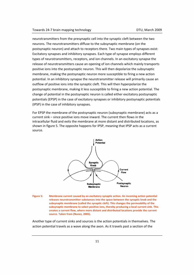
For EPSP the membrane of the postsynaptic neuron (subsynaptic membrane) acts as a current sink – since positive ions move inward. The current then flows in the intracellular fluid and exits the membrane at more distant and distributed locations, as shown in figure 5. The opposite happens for IPSP, meaning that IPSP acts as a current source.
Figure 5: Membrane current caused by an excitatory synaptic action. An incoming action potential releases neurotransmitter substances into the space between the synaptic knob and the subsynaptic membrane (called the synaptic cleft). This changes the permeability of the subsynaptic membrane to select positive ions, thereby producing a local current sink. This creates a current flow, where more distant and distributed locations provide the current source. Taken from (Nunez, 2005).
Another type of current sinks and sources is the action potentials in themselves. The
action potential travels as a wave along the axon. As it travels past a section of the

Towards 24-7 brain mapping technology DTU, March 2009
12
membrane an inflow of mostly Na+ ions happens. This inflow of ions functions as a
current sink. After the action potential has travelled past the section of membrane an
outflow of mostly K+ ions happen to reestablish the membrane potential. Thus the
propagation of an action potential can be seen as a current sink which is travelling fast
along an axon followed closely by a current source. Many axons are covered by an
electrically insulating material called a myelin sheath. Along the length of the axon are
regular points at which the axon is not covered by the myelin sheath (called nodes of
Ranvier – see also Figure 1). The action potential cannot travel through the membrane
covered in myelin. Instead the action potential jumps from one node of Ranvier to the
next (called saltatory conduction).
Many other processes in the brain can also influence the potential. But these are
believed to be less important for generating a potential (Nunez, 2005). Below some of
them are mentioned:
Active or passive transport of ions across the membrane, e.g. in order to re-establish ion concentrations inside the cell after an action potential.
Electrical synapses where neurons connect mechanically and electrically.
Reciprocal synapses which are synapses between dendrites.
Fast chemical transport where the membranes of adjacent neurons connect directly creating a “short-circuit”.
Retrograde signalling where postsynaptic neurons release substances which prevent the release of neurotransmitters from the presynaptic neuron.
2.4 From current sources to scalp potential Now that we have looked at what the sources of potential inside the brain are, we need
to integrate that knowledge into an understanding of how the sources create the
potential measured at the scalp. Of all the possible sources mentioned in the previous
section the action potential and the synapses are the ones likely to be important at the
scalp level.
It is generally accepted that action potentials only contribute locally to the potential but
not at scalp level. There are several explanations for this: Only if a large number of
action potentials happen concurrently is the effect measurable at the surface of the
scalp. Since action potentials have very short duration the probability of the action
potentials happening at the same time is small. Another issue is the distribution of the
sources and sinks. Axons in the neocortex are not unidirectional with respect to the
surface of the brain. Therefore they will most likely cancel each other out. Axons also
form fibers containing a number of axons. The longest and most numerous of these

Towards 24-7 brain mapping technology DTU, March 2009
13
fibers – the corticocortical fibers that travel through the white matter – are much more
distant from the surface of the scalp, and will thus only produce a negligible potential.
This leaves us with the IPSP and EPSP as respectively current source and sink. As
suggested earlier the magnitude of electric potential or dipole moment at distance
depends heavily on distribution and synchrony. It is known from anatomical data that
inhibitory and excitatory synapses are distributed in a specific way (Megias, Emri,
Freund, & Gulyas, 2001). Almost all synapses close to the cell bodies are inhibitory
synapses. In the dendritic tree which is closer to the cortex surface mostly excitatory
synapses are seen. Since the cortex is 2-4 mm deep, this leads to a separation of the
current source and sinks on the same order of scale. The spatial distribution of the
synapses gives the effect of a dipole placed normal to the local cortical surface.
As mentioned earlier little or no potential is found perpendicular to the axis of a dipole.
Because the surface of the cortex is folded, a greater contribution to the scalp potential
is received from areas where the cortex is parallel with the surface of the scalp. As seen
on figure 6 the cortex is parallel to the scalp surface roughly at top of the gyri and at the
bottom of the sulci (Srinivasan, Winter, Ding, & Nunez, 2007). The distance from the top
of the gyri to the bottom of the sulci is in the order of a cm or more. The shortest
distance between scalp surface and the top of the gyri is about 1-1.5 cm. As the
potential drops off with the square of the distance, a doubling of the distance means
only ¼ of the potential. Consequently most of the measured EEG signal is likely to
originate from the cortical surface on the top of the gyri (Nunez, 2005).
Figure 6: Drawing of the cortex in relation to the skull and scalp. The triangles in the cortex signify pyramidal cells. The figure shows that the orientation of the pyramidal cells with respect to the surface of the scalp varies with the location in the cortex. The axis of the pyramidal cells are perpendicular to the scalp surface at the top of the gyri. At some locations between the gyri and sulci the pyramidal cells are parallel with the scalp surface.

Towards 24-7 brain mapping technology DTU, March 2009
14
Next we take a look at the synchrony between the sources measured by a value called
the coherence. Scalp potential amplitude depends strongly on the amount of source
synchronization because the individual contributions sum up, but naturally only if
synchronous. A single macrocolumn containing about 100,000 pyramidal cells is not able
to produce a dipole moment strong enough to produce scalp potentials. As a rough
estimate synchronous activity is needed in about 6 cm2 of cortex (approx. 600
macrocolumns or 60,000,000 neurons) located on the gyri in order to produce
recordable scalp potentials.
Using equation 2.7 we can estimate the ratio between cortical potential and scalp
potential. Looking at a single dipole in the cortex the distance to the surface of the
cortex would be in the order of a few mm and the distance to the scalp surface would be
1-2 cm. The ratio is then in the order of 100 ((10 mm)2/(1 mm)2). More realistically, the
potential is generated by many synchronous dipoles over a larger area. For such a dipole
layer it can be shown that the ratio between cortical potential and scalp potential
becomes smaller with increasing area of dipoles (Nunez, 2005). This relationship is
shown in figure 7.
Figure 7: Theoretical estimates of ratio between cortical and scalp potential as a function of area size of synchronously active cortex. A larger area of synchronously active dipoles decreases this ratio. The three curves are for the skull to brain resistivity ratios shown in the figure (40, 80, and 120). Two known experimental data points are also plotted in the figure. Reproduced from (Nunez, 2005).
2.5 Measuring the EEG An EEG consists of the measured potential difference between two electrodes placed
different places on the scalp. One of the electrodes is called the reference electrode and
the other the recording electrode. When using many electrodes usually the same

Towards 24-7 brain mapping technology DTU, March 2009
15
reference electrode is used for each of the recording electrodes. Calling this single
electrode a reference electrode is perhaps a bit misleading as the potential variations
occurring in this electrode affects the measured signal as well. Other types of electrode
references are also used. One commonly used is the average reference where the
outputs of all the electrodes are averaged, and the averaged signal is used as reference
for each of the electrode channels.
In a clinical setting when recording a routine EEG 21 to 25 electrodes are used (including
reference and ground electrode) (Nunez, 2005). EEG recorded with many more
electrodes is also being used today, mostly for research purposes. Systems with up to
256 electrodes have been developed.
When recording an EEG it is estimated that a single electrode channel records average
synaptic action from 100 million to 1 billion individual neurons. There is still room for
improvement in this respect but not much. The theoretical limit for distance between
electrodes is 1 cm which would record averages of “only” 10 million neurons. (Nunez,
2005)
The advantage of EEG does not lie in its spatial resolution which as can be seen is rather
poor compared to the array of other neuroscience tools available such as PET, SPECT,
fMRI and microelectrode recordings. The main strength of EEG lies in the quantification
of spatio-temporal patterns with excellent temporal and mediocre (or worse) spatial
resolution. High spatial resolution and precise source localization is not a natural
application of EEG. The signal from the electrodes can be sampled at almost any
frequency down to the millisecond level and below. In clinical EEG a sampling frequency
of typically 200 or 256 Hz is used (Nuwer, et al., 1998).
When using EEG systems with a large number of electrodes, several practical problems
present themselves. It becomes very time consuming to set up the recording.
Furthermore the amount of wires becomes very cumbersome for the subject.
Consequently, depending on the application it is not always desired to increase the
number of electrodes.
The measured potential at the scalp is 20-100 μV in amplitude (Aurlien, 2004). This faint
signal is easily drowned out by the many sources of noise. Many sources of noise giving
rise to artifacts in the measured signal are generated by the body itself. Some common
types of artifacts are eye-induced artifacts (blinking and eye movement), muscle induced
artifacts, and cardiac artifacts. Artifacts from other sources include movement of the
electrodes, poor grounding from power line noise, and poor contact with the skin
particularly when the subject is sweating.

Towards 24-7 brain mapping technology DTU, March 2009
16
As mentioned in the introduction a company called Hypo-Safe is developing a device
which takes a new approach at recording the EEG. Figure 8 shows a concept drawing of
the device. The idea of the device is to implant the electrode and recording device fully
under the skin. The device consists of an electrode attached to a small recording device
which is implanted fully under the skin. On the outside of the skin, a device resembling a
hearing aid is placed behind the ear. This device collects the recorded information.
(Hypo-Safe, 2009)
The advantages of implanting the EEG device subcutaneously are many. All the problems
with establishing and maintaining proper skin contact are eliminated. Another
advantage is that the device can be carried by the subject 24 hours a day for years
without compromising the comfort of the user. This allows for long-term recordings of
under normal life conditions.
Figure 8: The EEG recording device being developed by Hypo-Safe. The device consists of two parts. The part with the electrode is implanted under the skin and the second part, which is placed behind the ear, collects the recorded signal.
2.6 Characteristics of the EEG In order to use the EEG in practice it is often necessary to look at specific features of the
signal. The features can either be used to obtain a better understanding or model of a
specific signal, or the features can be used as an input to a classification algorithm. This
section describes some different characteristics of the EEG signal.

Towards 24-7 brain mapping technology DTU, March 2009
17
In general the EEG signal can be divided into rhythmic/spontaneous activity and
transient activity. The spontaneous activity occurs in the absence of any sensory stimuli,
while transient activity happens as a response to a stimulus.
2.6.1 EEG rhythms/spectral information
The rhythmic activity in the brain can be divided into characteristic frequency bands. The
limits between these frequency bands are not set in stone but vary between individual
subjects (especially due to age), as well as other influences such as use of drugs. Table 1
summarizes the different bands, their frequency range, their spatial location, and under
which circumstances the activity is seen.
In general the amplitude of EEG decreases with increasing frequency.
Type Frequency
(Hz)
Location Conditions for activity
Delta up to 4 frontally in adults, posterior in
children
adults slow wave sleep in babies
Theta 4 - 7 Hz young children drowsiness or arousal in
older children and adults idling
Alpha 8 - 13 Hz posterior regions of head, both
sides, higher in amplitude on
dominant side. Central sites (c3-
c4) at rest .
relaxed/reflecting closing the eyes
Beta 13 - 30 Hz both sides, symmetrical
distribution, most evident
frontally; low amplitude waves
alert/working active, busy or anxious
thinking, active concentration
Gamma 30 and up certain cognitive or motor functions
Table 1: Summary of the spectral bands in the rhythmic activity of EEG. The frequency limits for each band is an approximate value, because it varies over subjects and conditions. The location where each band is primarily seen is in the third column. The rightmost column states the conditions that normally increase activity of a given band. Summary of (Nunez, 2005) and (Wikipedia - Electroencephalography, 2009)
2.6.2 Mu rhythm
The mu rhythm is a spontaneous activity usually seen in the alpha range (8-13 Hz) over
the sensorimotor cortex. The amplitude of the signal is strongest when no movements

Towards 24-7 brain mapping technology DTU, March 2009
18
are performed. A decrease in amplitude is seen over the corresponding area in the
contralateral motor cortex when a movement is done. Even just thinking about doing a
movement (motor imagery) will decrease the amplitude of the mu rhythm.
(Pfurtscheller, Brunner, Schlogl, & Lopesdasilva, 2006)
2.6.3 ERP and EP
As mentioned, a stimulus can provoke a transient activity in the EEG. The measured EEG
signal can be timed to the stimulus event and is then called event related potentials
(ERP). Usually it is difficult to see any actual change in the EEG from a single stimulus
event. But if many trials are conducted and the results averaged, the random (untimed)
activity of the brain is averaged out and only the time-locked part caused by the
stimulus event remains. An example of an ERP is seen in figure 9. Depending on the
conditions for the recording and the location of the recording a number of peaks are
seen in the ERP. Ordinarily these peaks are referred to by a letter indicating polarity
(negative (N) or positive (P)) and a number indicating the latency from the event in
milliseconds. For example, P300 is a positive peak occurring 300 ms after the event.
Figure 9: Example of an event related potential (ERP) showing the typical components encountered. Notice that the vertical axis is reversed on the plot – this is due to historic reasons.
The immediate and spontaneous change recorded after an event is called an evoked
potential (EP). The EP reflects the processing of the sensory stimulus by the brain. An
example of an EP is the visual evoked potential (VEP), which is caused by stimulation of
the subject’s visual field. Figure 10 shows a normal VEP performed by a paradigm set out
in the visual evoked potential standard (Odom, et al., 2004). As can be seen from the
figure, the peaks are all located within the first few hundred milliseconds after the
stimulus event – this is a general characteristic for EPs.

Towards 24-7 brain mapping technology DTU, March 2009
19
Figure 10: A normal visual evoked potential (VEP) recorded from a subject looking at a checkerboard pattern where the colors are reversed 1-3 times a second (Odom, et al., 2004).
2.6.4 Readiness potential
The readiness potential (RP) is also called premotor potential or bereitschaftspotential.
The RP is an activity that occurs contralateral in the motor cortex before the actual
voluntary muscle movement is performed. The magnitude of the RP is quite small and
can only be visualized by averaging (Fabiani, Gratton, & Coles, 2000).
2.6.5 ERD, ERS, and ERSP
When calculating the ERP, a model consisting of a time-locked signal (the ERP) added to
uncorrelated noise is assumed. By averaging the individual events all activity that is not
both time-locked and phase-locked is averaged out through phase cancellation. This
simple model is useful and sufficient in some respects, but sometimes the desired part
of the signal is averaged out by this simple averaging method.
It has been shown that some events cause a change that is time-locked to the event but
not phase-locked. This type of event is believed to be caused by a decrease or increase
in synchrony between the individual neurons. A decrease in synchronization is called
event related desynchronization (ERD) and an increase in synchronization is called event
related synchronization (ERS) (Pfurtscheller & Lopes da Silva, 1999). An ERD or ERS might
not be phase-locked to the event; therefore it might not be seen on the ERP. But an ERD
or ERS would cause a decrease or an increase in power of a given frequency band.
In order to quantify ERD and ERS in the time domain several methods are being used.
The one used in this work is called event related spectral perturbation (ERSP) (Makeig S.
, 1993). The ERSP measures average changes in amplitude of the frequency spectrum
relative to the baseline before the event. The average changes are plotted as a function
of time from the event. The calculation of ERSP is described further in section 3.2.2.

Towards 24-7 brain mapping technology DTU, March 2009
20
3 Methods and tools
3.1 Classification When measuring an EEG you will often have large amounts of data, in particular if the
recording is done over a long time period. To extract information about such a large
amount of data automated methods are needed. Automated methods are also needed
for a real time BCI system.
A common problem when looking at EEG data is to work out if a certain observation can
tell us something about the conditions under which the observation is made. For
instance to detect whether a diabetes patient has critically low blood sugar or not based
on an EEG measurement.
In general, the area concerning development of algorithms which can tell us something
about the organization of data is called machine learning. The purpose of the algorithms
is to make a model of the data. When new data is encountered the rules of the model
can then give us information about the data.
Several branches of machine learning exist. One branch is the unsupervised learning.
Here an algorithm tries to determine the organization of the data by using only the data
itself, i.e. without knowledge of the source signals or the process by which the data is
mixed. An example of unsupervised learning is independent component analysis.
Another branch of machine learning is supervised learning. In this case some sort of
knowledge about the data is at hand. The knowledge can for instance be information
about the circumstances under which a specific EEG is measured. In other words a given
observation is supplied with a label containing information about the observation. If a
number of observations are available, this set of observations and labels can be used to
train a function. The input to the function is the observation and ideally the output is the
label. This function or model can then be supplied with new observations not used in
the training process and hopefully supply the correct label.
In this section two different classification methods are presented. A simple linear
classifier called Fisher’s linear discriminant (FLD) and a more complex linear classifier
called support vector machines (SVM). SVM can be extended into a non-linear classifier.
This non-linear SVM, called Gaussian SVM, is also presented.
FLD was chosen as it is a very common method used with success in many BCI systems
(Lotte, Congedo, Lécuyer, Lamarche, & Arnaldi, 2007). Furthermore, the classifier is
simple to apply, and only uses little computational power. The drawback of the method

Towards 24-7 brain mapping technology DTU, March 2009
21
is that it is linear and does not cope well with nonlinear data. Linear SVM is selected
because it, unlike FLD, is insensitive to high-dimensional data (Lotte, Congedo, Lécuyer,
Lamarche, & Arnaldi, 2007). Furthermore it can be customized to the data used by
changing an adjustable parameter. Because EEG data often can be of non-linear nature,
Gaussian SVM is also tried.
In general for all the presented algorithms we can consider a set of (training) data
T= {(𝒙𝑘 ,𝑦𝑘),… , (𝒙𝑘 ,𝑦𝑘)}, containing k pairs of observation/feature vectors 𝒙𝑖 ∈ ℝ𝑛 and
the class label for each of the k observations, 𝑦𝑖 ∈ 𝒴. In the classification problems
looked at in this work, only one of two labels is possible for each observation – thus only
the binary case of 𝒴 = {1,2} is considered. We then want to find a classification rule, q,
which is able to predict the label only using the information given in the observation,
𝑞:𝒳 → 𝒴 = {1,2}. The classification rule can then be used to predict the labels of any
new observation from the same distribution.
3.1.1 Fisher’s linear discriminant (FLD) classification
Fisher’s linear discriminant classification was presented by the statistician and biologist
Sir Ronald Aylmer Fisher in 1936 (Wikipedia - Linear discriminant analysis, 2009). The
implementation used in this work, is from the statistical pattern recognition (STPR)
toolbox for Matlab (Franc & Hlavac, 2008)
This supervised method for classification is based on a simple linear weighing of the
features or observations, with the discriminant function being:
𝑓 𝒙 = 𝒘 ∙ 𝒙 + 𝑏 (3.1)
defined by the parameter or weight vector 𝒘 ∈ ℝ𝑛 and bias 𝑏 ∈ ℝ. The assignment of a
label to a given observation is then done by the following rule q,
𝑞 𝒙 =
1 if 𝑓 𝒙 = 𝒘 ∙ 𝒙 + 𝑏 ≥ 0
2 if 𝑓 𝒙 = 𝒘 ∙ 𝒙 + 𝑏 < 0 (3.2)
In other words we want to separate the points of the two classes with a hyperplane. In
order to find the hyperplane that best divides the two classes, we define the class
separability as a function of 𝒘:
𝐹 𝒘 =
𝒘 ∙ 𝑺𝑩𝒘
𝒘 ∙ 𝑺𝑾𝒘 (3.3)
where 𝑺𝑩 is the scatter matrix between the classes: 𝑺𝑩 = 𝝁1 − 𝝁2 (𝝁1 − 𝝁2)𝑇 (𝝁𝒚 is a
vector of the means of observations). 𝑺𝑾 is the scatter matrix within the classes defined
as:

Towards 24-7 brain mapping technology DTU, March 2009
22
𝑺𝑾 = 𝑺𝟏 + 𝑺𝟐, 𝑺𝑾 = 𝒙𝑖 − 𝝁𝑖 (𝒙𝑖 −
𝑖∈𝒴𝑦
𝝁𝑖)𝑇 ,
𝑦 ∈ {1,2}
(3.4)
We then want to find the parameter vector 𝒘 which maximizes the class separability.
Several solutions to this problem are being used. In the implementation used in this
work the following solution is used:
𝒘 = 𝑺𝑾−1(𝝁1 − 𝝁2) (3.5)
In order to find the full discriminant function we also need to find 𝑏. In the used
implementation this is done by solving
𝒘 ∙ 𝝁𝟏 + 𝑏 = − 𝒘 ∙ 𝝁𝟐 + 𝑏 ⇒
𝑏 = −0.5 ∗ (𝒘 ∙ 𝝁𝟏 + 𝒘 ∙ 𝝁𝟐) (3.6)
3.1.2 Support vector machine (SVM) classification
Support vector machines are a group of supervised classification methods. The original
method was presented by Vladimir Vapnik in 1963 (Wikipedia - Support vector machine,
2009). The basis for this method is, like the FLD classifier, to find a hyperplane which
separates the two classes. The idea of SVM is to maximize the margin between the
hyperplane and the points of the two datasets closest to the dividing hyperplane. A
dataset that is linearly separable have many hyperplanes that will correctly classify all
the training data. The approach used by SVM will ensure that the found hyperplane will
also classify future observations (test data) as correctly as possible.
The data points closest to the boundary between the two classes are the only ones that
contribute to the location of the hyperplane. These “deciding” data points are called
support vectors.
Originally SVM was only a linear classification method, but the method has later been
extended to also work as a non-linear classifier.
The implementation of SVM used in this work is from the STPR toolbox for Matlab (Franc
& Hlavac, 2008).
Linear classifier
The linear SVM uses the same discriminant function as FLD, namely:

Towards 24-7 brain mapping technology DTU, March 2009
23
𝑓 𝒙 = 𝒘 ∙ 𝒙 + 𝑏 (3.7)
The classification rule in the binary case is also the same as for FLD:
𝑞 𝒙 =
1 if 𝑓 𝒙 ≥ 0
2 if 𝑓 𝒙 < 0 (3.8)
The difference between the two methods is, as mentioned, in the way the hyperplane is
found. When the data is completely separable by a hyperplane, the so-called hard
margin SVM can be used. In this case all data points are used when calculating the
weight and bias. In many cases this is not desirable since excluding a few outliers can
improve the margin considerably. Furthermore, when dealing with data that is not
linearly separable, it is necessary to allow the classifier to misclassify data points in order
to find a hyperplane at all. The practice of allowing the classifier to misclassify some data
points is called soft margin SVM.
When using the soft margin SVM the optimal parameters 𝒘∗ and 𝑏∗ corresponding to
the maximum margin hyperplane is calculated by solving the following quadratic
programming optimization problem:
minimize:
𝒘,𝑏
1
2 𝒘 2 + 𝐶 𝜉𝑖
𝑙
𝑖=1
subject to: 𝒘 ∙ 𝒙𝒊 + 𝑏 ≥ +1 − 𝜉𝑖 , 𝑖 ∈ ℐ1
𝒘 ∙ 𝒙𝒊 + 𝑏 ≤ −1 + 𝜉𝑖 , 𝑖 ∈ ℐ2
𝜉𝑖 ≥ 0, 𝑖 ∈ ℐ1 ∪ ℐ2
(3.9)
𝜉𝑖 ≥ 0 are slack variables, which will allow observations to be misclassified. ℐ1 =
𝑖: 𝑦𝑖 = 1 and ℐ2 = 𝑖:𝑦𝑖 = 2 are sets of indices for the two classes in the training
data. The regularization constant 𝐶 > 0 defines the importance of the slack variables. A
large value of C means that classification errors incur a large penalty – setting C to
infinity gives the same results as using a hard margin SVM. Setting a smaller value of C
lets more data points close to the boundary be ignored and thus creates a larger margin.
It should be noted here that the scale of C has no direct meaning. It is therefore not
intuitively easy to set the value of the regularization parameter. An illustration of the
effect brought about by changing the regularization parameter is shown in figure 11.

Towards 24-7 brain mapping technology DTU, March 2009
24
Figure 11: The effect of changing the regularization parameter C on the decision boundary when using linear SVM. Synthetic data is used. The support vectors are marked with a black circle. The C values used are left: C=1, middle: C=10, and right C= 100. Using a low C-value of 1 increases the margin and allows the classifier to ignore the points close to the boundary. In this case the low C-value allows the classifier to put all data points within the margin and a poor result is obtained as two data points are misclassified. By increasing the C-value the margin becomes narrower and fewer points are used as support vectors. With a C-value of 100 only the four closest points are used as support vectors and only the one misclassified data point is within the margin.
Non-linear classifier
For some problems a linear classifier will yield unsatisfactory results, simply because
they have non-linear decision boundaries. As mentioned earlier SVM classification can
be extended to take care of non-linear problems as well. The procedure for doing this is
to map the data to another vector space using a so-called kernel-function 𝒌𝑆.
The discriminant function then becomes:
𝑓 𝒙 = 𝜶 ∙ 𝒌𝑠 𝒙 + 𝑏 (3.10)
𝜶 ∈ ℝ𝒍 is a vector containing weights and 𝑏 ∈ ℝ is the bias. The data vector is mapped
into another space using a kernel function 𝒌𝑠 𝒙 = [𝑘 𝒙, 𝒔1 ,… ,𝑘 𝒙, 𝒔𝑑 ]𝑇. The support
vectors 𝒮 = {𝒔1 ,… , 𝒔𝑑} is the subset of training vectors used when calculating the
discriminant function. Many different kernel functions can be used. In this work only
one kernel function has been selected, namely the widely used Gaussian kernel function
(also called radial basis function (RBF)) – SVM classification using this kernel is called
Gaussian SVM. The Gaussian kernel is described by the function
𝑘 𝒙, 𝒔 = exp −
𝒙 − 𝒔 2
2𝜎2 (3.11)
The parameter 𝜎 > 0 in this kernel function determines how wide the Gaussian function
centered on each of the support vectors is. When the squared distance 𝒙 − 𝒔 2 is

Towards 24-7 brain mapping technology DTU, March 2009
25
much larger than 2𝜎2 the function is close to zero. If σ is set to a high value the Gaussian
“bump” around each support vector will be relatively wide and vice versa. When using a
high σ the entire set of support vectors will thus influence a given data point, leading to
a smoother decision boundary. If σ is set lower, the Gaussian becomes more narrow
leading to a possibility for greater bends in the decision boundary. If σ is set too low, the
discriminant function will essentially be zero outside the close vicinity of each of the
support vectors. The decision boundary will then most likely lie close to the support
vectors leading too poor classification for new observations. An illustration of the effect
of changing σ is shown in figure 12.
Figure 12: The effect of changing the σ parameter when using Gaussian SVM. The data used in this figure is the same as the data used in figure 11. The σ-values used are: left: σ=5, middle plot: σ=1, and right plot: σ=0.2. When using a high σ-value in the left plot, the decision boundary is only allowed a slight curve, and the result is close to a linear classifier. Using a σ-value of 1 is just the right setting as a perfect decision boundary is achieved. If the σ-value is set too low (right plot), then the decision boundary can curve too much and the data is overfitted. Although this gives a perfect classification for the training data, a poor classification of any test data will probably be seen.
Training of the binary non-linear SVM equates to solving the following quadratic
programming problem.
maximize:
𝜷∗𝜷 ∙ 𝟏 −
1
2𝜷 ∙ (𝑯𝜷)
subject to: 𝜷 ∙ 𝜸 = 1
𝜷 ≥ 𝟎
𝜷 ≤ 𝟏𝐶
(3.12)
0 is vector of zeros size [l x 1], 1 is a vector of ones size [l x 1]. γ and H are defined as
follows:

Towards 24-7 brain mapping technology DTU, March 2009
26
𝛾𝑖 = 1 if 𝑦𝑖 = 1−1 if 𝑦𝑖 = 2
𝐻𝑖,𝑗 = 𝑘 𝒙𝑖 ,𝒙𝑗 if 𝑦𝑖 = 𝑦𝑗
−𝑘 𝒙𝑖 ,𝒙𝑗 if 𝑦𝑖 ≠ 𝑦𝑗
The weight vector 𝜶 in the discriminant function is then found as
𝛼𝑖 = 𝛽𝑖 if 𝑦𝑖 = 1−𝛽𝑖 if 𝑦𝑖 = 2
The bias 𝑏 can be found from the Karush-Kuhn-Tucker (KKT) conditions where the
following constraints must hold for the optimal solution:
𝑓 𝒙𝒊 = 𝜶 ∙ 𝒌𝒔 𝒙𝒊 + 𝑏 = +1 for 𝑖 ∈ {𝑗:𝑦𝑗 = 1, 0 < 𝛽𝑗 < 𝐶
𝑓 𝒙𝒊 = 𝜶 ∙ 𝒌𝒔 𝒙𝒊 + 𝑏 = −1 for 𝑖 ∈ {𝑗:𝑦𝑗 = 2, 0 < 𝛽𝑗 < 𝐶
𝑏 is then found as an average over all the constraints so that
𝑏 =
1
ℐ𝑏 𝛾𝑖 − 𝜶 ∙ 𝒌𝒔 𝒙𝒊
𝑖∈ℐ𝑏
(3.13)
where the indices of the vectors on the boundary are denoted by ℐ𝑏 = {𝑖: 0 < 𝛽𝑖 < 𝐶}.
3.1.3 Cross-validation
After training a classifier on a training data set, you will want to test it afterwards on a
new data set which the classifier has not used during the training. This is done to assess
how accurate the classifier is and to estimate how well it will perform in practice. Often
the number of observations you have available for training and testing the classifier is
very limited. With a given amount of observations you would want to use as many of the
observations as possible to train a perfect classifier, but this would leave you with too
few observations to properly evaluate the classifier afterwards.
In order to alleviate this issue, cross-validation methods are used. The principle behind
this is to partition the entire amount of observations into a training subset and a test
subset. After having trained and tested a classifier, a new partitioning of the
observations is made. The new subsets are then used to train and test a new classifier.
This is repeated a number of times. The validation results are then averaged over the
individual rounds.
Many types of cross-validations are in use. In this work leave-one-out (LOO) cross-
validation is used (presented in (Lunts & Brailovskiy, 1967)). As the name suggest this
method involves taking out a single observation for test data set and using all the rest as
training data set. This is repeated so that each observation will be tested once. This is
Towards 24-7 brain mapping technology DTU, March 2009
27
the most thorough of the cross-validation methods and is only used for relatively small
data sets.
3.2 EEGLAB Most of the processing and visualization of the data in this work is done in the MATLAB
toolbox called EEGLAB (Delorme & Makeig, 2004). This toolbox simplifies many
commonly used procedures when working with EEG data, as well as offering many
different visualization options. Below, some of the visualizations used in this work are
presented.
3.2.1 ERP images
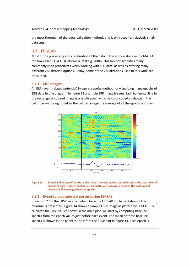
An ERP (event related potential) image is a useful method for visualizing many epochs of
EEG data in one diagram. In figure 13 a sample ERP image is seen. Each horizontal line in
the rectangular colored image is a single epoch which is color coded as shown in the
color bar on the right. Below the colored image the average of all the epochs is shown.
Figure 13: Sample ERP image of a surface electrode. The rectangular colored image at the top shows all epochs of data – epoch number is seen on the vertical axis to the left. The bottom plot shows the ERP averaged over all epochs.
3.2.2 Event related spectral perturbation (ERSP)
In section 2.6.5 the ERSP was described, here the EEGLAB implementation of this
measure is presented. Figure 14 shows a sample ERSP image as plotted by EEGLAB. To
calculate the ERSP values shown in the main plot, we start by computing baseline
spectra from the epoch values just before each event. The mean of these baseline
spectra is shown in the panel to the left of the ERSP plot in figure 14. Each epoch is

Towards 24-7 brain mapping technology DTU, March 2009
28
divided into overlapping time windows. A moving average of the amplitude spectrum of
these windows is found. Each of the found amplitude spectra is then divided by the
respective mean baseline spectrum in order to normalize them. Now that we have a
time-frequency decomposition of each trial, we can average them to obtain the ERSP
which is plotted in the figure. Below the main ERSP plot in figure 14 is shown the
minimum and maximum values of the ERSP plot. All the spectra can be calculated either
by FFT or by wavelet transform. The former is used in all cases in this work.
Figure 14: Event related spectral perturbation (ERSP) image. The plot is based on 280 trials of hand and foot motor imagery tasks from the data set used in section 4.3. The plot is calculated from electrode C3, i.e. over the hand motor cortex. The main plot shows the ERSP values in dB with the mean baseline spectral activity subtracted. The panel to the left of the ERSP plot presents the mean spectrum values during the baseline period, i.e. the values subtracted from the values in the ERSP plot. The panel below the ERSP image shows the maximum (green) and minimum (blue) ERSP values relative to baseline power at each frequency.
3.2.3 ICA
ICA decomposition is done with the EEGLAB method “runica”. This method is based on
the Extended Infomax algorithm (Lee & Sejnowski, 1998). The original Infomax algorithm
was presented in (Bell & Sejnowski, 1995). The implementation used in EEGLAB is
presented in (Makeig, Bell, Jung, & Sejnowski, 1996).
Towards 24-7 brain mapping technology DTU, March 2009
29
4 Data analysis
4.1 Comparison of subcutaneous electrodes with conventional
electrodes Currently, knowledge about the use of subcutaneous electrodes is almost non-existing.
Only one reference to the practical use of subcutaneous electrodes can be found in the
literature (Kamphuisen, et al., 1991). Although this reference states that the EEG
observed by the subcutaneous electrodes is similar to the EEG from ordinary skin
electrodes, no evidence is presented for the basis of this similarity. When contemplating
the use of subcutaneous electrodes for a variety of applications, a better understanding
of the differences in relation to ordinary (well known) electrodes is advantageous.
Using EEG data recorded simultaneously by subcutaneous electrodes and ordinary
surface electrodes, this section will focus on a comparison of the two types of electrodes
by various methods.
4.1.1 Description of dataset
The used data is a visual evoked potential (VEP) experiment which was carried out by
HypoSafe A/S at Odense University Hospital (OUH) on the 13th of December 2007.
Prior to the experiment, a subcutaneous electrode with four contact points was inserted
in the subcutis layer in the back of the head (visual area). The electrode was inserted
vertically in the center, due to constraints associated with blood vessel locations. Four
surface electrodes were placed on top of the subcutaneous ones, to allow for
comparison. In addition to the 2 times 4 electrodes, two reference electrodes were
placed on the top of the head (approx Cz), one for each set (one subcutaneous and one
surface). Both subcutaneous and surface electrodes are recorded with the same
equipment.
The full recording consists of approx. 6 minutes of EEG, where the subject is looking at a
computer screen. During three intervals, with breaks in between, the screen is flickering
a chessboard like image. The colours of the chessboard are changing with a frequency of
2 Hz (500 ms between the changes).
The datafile contains 9 signals: The first four channels are the surface channels; the fifth
channel is the stimulus channel (500 ms between events); the following four channels
are the subcutaneous channels. The sampling rate, fS = 256Hz.]
4.1.2 Preprocessing
The data is processed in the following way:
Towards 24-7 brain mapping technology DTU, March 2009
30
1. Data is imported into EEGLAB.
2. The event latencies are extracted from the stimulus channel.
3. 50 Hz noise is filtered out using a non-linear infinite impulse response (IIR) filter.
4. The data is divided into epochs based on the event data. Epoch start is set to
200 ms before the event and epoch end is set to 500 ms.
5. In order to remove low frequency drifts and like artifacts, a mean baseline value
(based on the -200 to 0 ms interval) is calculated and subtracted from each
epoch individually.
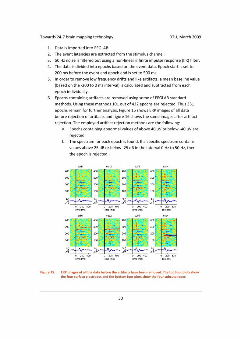
6. Epochs containing artifacts are removed using some of EEGLAB standard
methods. Using these methods 101 out of 432 epochs are rejected. Thus 331
epochs remain for further analysis. Figure 15 shows ERP images of all data
before rejection of artifacts and figure 16 shows the same images after artifact
rejection. The employed artifact rejection methods are the following:
a. Epochs containing abnormal values of above 40 μV or below -40 μV are
rejected.
b. The spectrum for each epoch is found. If a specific spectrum contains
values above 25 dB or below -25 dB in the interval 0 Hz to 50 Hz, then
the epoch is rejected.
Figure 15: ERP images of all the data before the artifacts have been removed. The top four plots show the four surface electrodes and the bottom four plots show the four subcutaneous
Towards 24-7 brain mapping technology DTU, March 2009
31
electrodes. Data from electrodes which are positioned on top of each other on the head are shown above and below each other in the plots above.
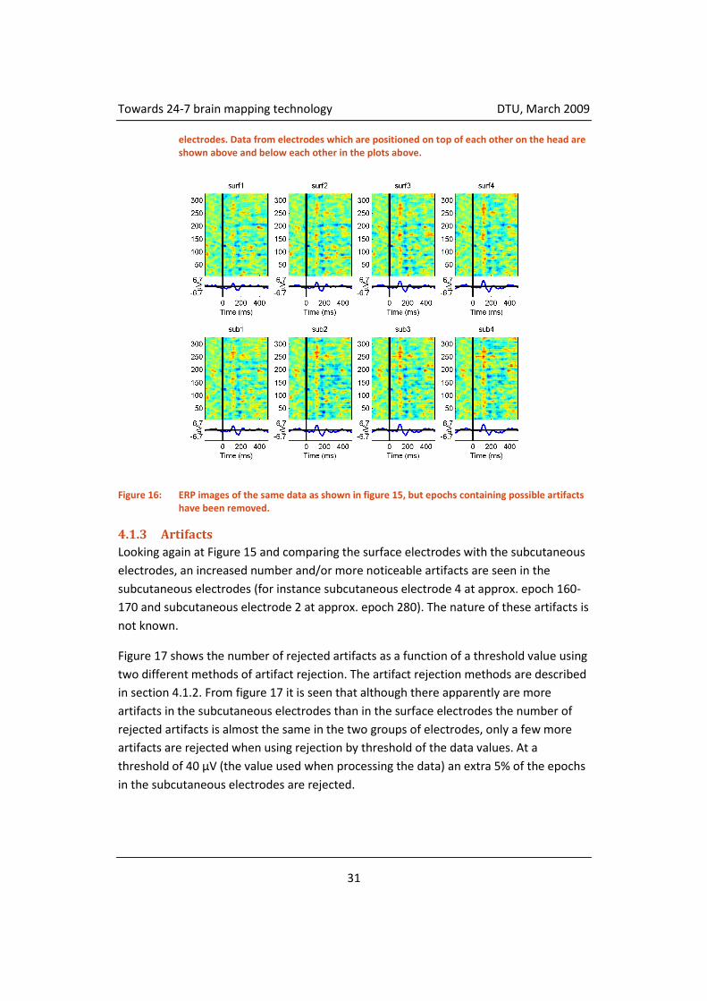
Figure 16: ERP images of the same data as shown in figure 15, but epochs containing possible artifacts have been removed.
4.1.3 Artifacts
Looking again at Figure 15 and comparing the surface electrodes with the subcutaneous
electrodes, an increased number and/or more noticeable artifacts are seen in the
subcutaneous electrodes (for instance subcutaneous electrode 4 at approx. epoch 160-
170 and subcutaneous electrode 2 at approx. epoch 280). The nature of these artifacts is
not known.
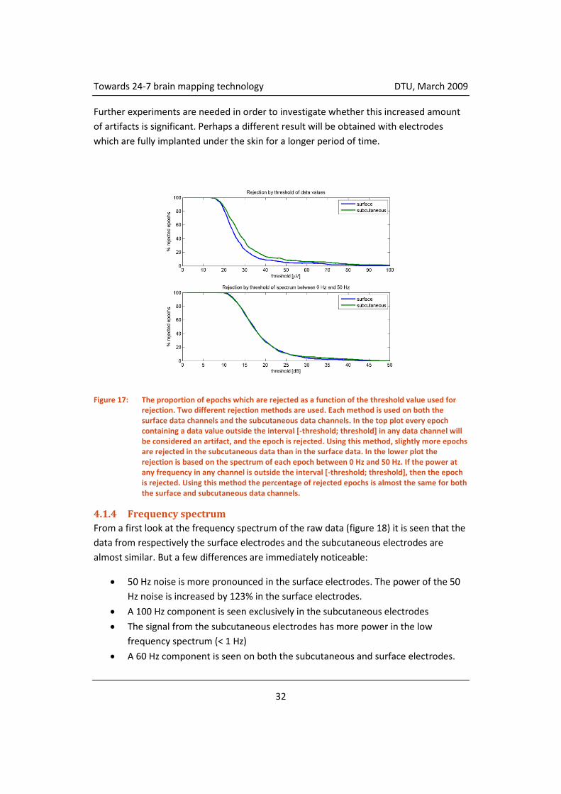
Figure 17 shows the number of rejected artifacts as a function of a threshold value using
two different methods of artifact rejection. The artifact rejection methods are described
in section 4.1.2. From figure 17 it is seen that although there apparently are more
artifacts in the subcutaneous electrodes than in the surface electrodes the number of
rejected artifacts is almost the same in the two groups of electrodes, only a few more
artifacts are rejected when using rejection by threshold of the data values. At a
threshold of 40 μV (the value used when processing the data) an extra 5% of the epochs
in the subcutaneous electrodes are rejected.
Towards 24-7 brain mapping technology DTU, March 2009
32
Further experiments are needed in order to investigate whether this increased amount
of artifacts is significant. Perhaps a different result will be obtained with electrodes
which are fully implanted under the skin for a longer period of time.
Figure 17: The proportion of epochs which are rejected as a function of the threshold value used for rejection. Two different rejection methods are used. Each method is used on both the surface data channels and the subcutaneous data channels. In the top plot every epoch containing a data value outside the interval [-threshold; threshold] in any data channel will be considered an artifact, and the epoch is rejected. Using this method, slightly more epochs are rejected in the subcutaneous data than in the surface data. In the lower plot the rejection is based on the spectrum of each epoch between 0 Hz and 50 Hz. If the power at any frequency in any channel is outside the interval [-threshold; threshold], then the epoch is rejected. Using this method the percentage of rejected epochs is almost the same for both the surface and subcutaneous data channels.
4.1.4 Frequency spectrum
From a first look at the frequency spectrum of the raw data (figure 18) it is seen that the
data from respectively the surface electrodes and the subcutaneous electrodes are
almost similar. But a few differences are immediately noticeable:
50 Hz noise is more pronounced in the surface electrodes. The power of the 50
Hz noise is increased by 123% in the surface electrodes.
A 100 Hz component is seen exclusively in the subcutaneous electrodes
The signal from the subcutaneous electrodes has more power in the low
frequency spectrum (< 1 Hz)
A 60 Hz component is seen on both the subcutaneous and surface electrodes.

Towards 24-7 brain mapping technology DTU, March 2009
33
The 50 Hz noise might possibly be explained by radiation of line noise from the
surroundings. Because the subcutaneous electrodes are “protected” by a layer of skin,
they might be less influenced by this radiated line noise.
The 100 Hz component might be a harmonic of the 50 Hz noise, but why it is only seen in
the subcutaneous electrodes, and not in the surface electrodes where the 50 Hz noise is
larger, is unknown.
As described earlier, more artifacts of various kinds are seen in the subcutaneous
electrodes. This might be the reason for the higher power of the low frequency signal in
the subcutaneous electrodes.
The 60 Hz component is a component usually seen when using a power supply of this
frequency (i.e. in the United States). This cannot be the case in this experiment. The 60
Hz component might perhaps be caused by the update frequency of the computer
screen the test subject is looking at. This phenomenon is known as frequency driving.
Figure 19 shows the spectrum after having processed the data as described in section
4.1.2. From this graph a 9 Hz alpha activity is clearly seen. Furthermore a peak at around
26 Hz is seen, corresponding with high beta waves.

Towards 24-7 brain mapping technology DTU, March 2009
34
Figure 18: Plot of the frequency spectrum of the raw data, i.e. before filtering and removal of artifacts. The top plot displays the spectrum for the four surface electrodes. The bottom plot displays the spectrum for the four subcutaneous electrodes. Note the higher power of the low frequency components in the plot of the subcutaneous electrodes.
Figure 19: Frequency spectrum of processed data (see section 4.1.2 Preprocessing), i.e. after filtering of 50 Hz noise and removal of artifacts. The top plot displays the four surface electrodes. The bottom plot displays the four subcutaneous electrodes. Note the 60 Hz component in both plots and the 100 Hz component in the bottom plot.

Towards 24-7 brain mapping technology DTU, March 2009
35
4.1.5 Event related potentials (ERP)
Figure 20 shows the ERP for each of the eight electrodes. Some characteristic
components of the ERP are seen: A positive peak at 110 ms after visual stimulus (P110),
a negative peak at 170 ms (N170), and a (small) negative peak at 220 ms (P220).
From the plot in figure 20 some small differences between the subcutaneous and
surface electrodes can be seen. Larger amplitudes are seen in the subcutaneous
electrodes – most pronounced in electrode locations 1 and 2. The amplitude at the peak
at 110 ms is on average 19% larger in the subcutaneous electrodes compared to the
surface electrodes. In electrode 1 the amplitude is 37% larger in the subcutaneous
electrodes and in electrode 4 only a 1% increase is seen.
These larger amplitudes for the subcutaneous electrodes – which are closer to the
cortex of the brain – might be expected since the potential of a dipole falls off as the
inverse square of the distance (Nunez, 2005). The distance between the electrodes and
the cortex can be as little as 1 cm and with the thickness of the epidermis and dermis
being up to several millimeters, this decrease in distance could lead to a significant
increase in amplitude.
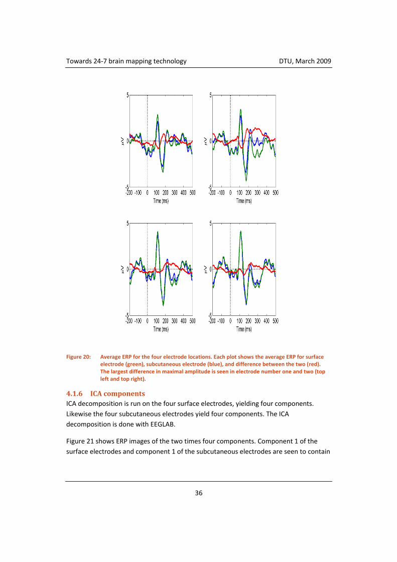
Towards 24-7 brain mapping technology DTU, March 2009
36
Figure 20: Average ERP for the four electrode locations. Each plot shows the average ERP for surface electrode (green), subcutaneous electrode (blue), and difference between the two (red). The largest difference in maximal amplitude is seen in electrode number one and two (top left and top right).
4.1.6 ICA components
ICA decomposition is run on the four surface electrodes, yielding four components.
Likewise the four subcutaneous electrodes yield four components. The ICA
decomposition is done with EEGLAB.
Figure 21 shows ERP images of the two times four components. Component 1 of the
surface electrodes and component 1 of the subcutaneous electrodes are seen to contain

Towards 24-7 brain mapping technology DTU, March 2009
37
most of the ERP. Figure 22 show the cross correlation between these two components –
a significant cross correlation coefficient of 86% is seen between the two components.
Figure 21: ERP images of ICA components. The four ICA components for the four surface electrodes are shown in the four top plots, and the four components for the four subcutaneous electrodes are shown in the bottom four plots.

Towards 24-7 brain mapping technology DTU, March 2009
38
Figure 22: The red curve shows the cross-correlation of ICA component one for subcutaneous electrodes and component one for surface electrodes (as shown in figure 21). The blue curve is constructed by calculating the cross-correlation between one of the components and a random permutation of the time indexes of the other component. 1000 different random permutations are made and the blue curve is the minimal and maximal values of the cross-correlation using these random permutations. The boundaries of the blue curve are then comparable to a significance level of 0.1%.
4.1.7 Conclusion on electrode comparison
This section has investigated the similarities and differences between surface electrodes
and subcutaneous electrodes used for measuring EEG.
The signals obtained using the two kinds of electrodes exhibited some small differences.
- Slightly more as well as more pronounced artifacts are seen in the subcutaneous
electrodes than in the surface electrodes. 14% of the epochs in the
subcutaneous electrodes compared to 9% of the epochs in the surface
electrodes are rejected when artifacts are rejected by threshold of the data
values. The cause for this increase in number of artifacts is unknown.
- Less 50 Hz noise is seen in the subcutaneous electrodes. The power of the noise
in the subcutaneous electrodes is reduced by 55% compared to the surface
electrodes. This is possibly due to a decreased effect of radiation of line noise
from the surroundings.

Towards 24-7 brain mapping technology DTU, March 2009
39
- Higher amplitude of the signal in the subcutaneous electrodes is seen. In
electrode 1 the peak amplitude at 110 ms is 37% higher in the subcutaneous
electrode compared to the surface electrode. This is most likely caused by the
subcutaneous electrodes simply being closer to the cerebral cortex.
When looking at the ICA components these also show a significant similarity between
the subcutaneous and the surface electrodes. When comparing the primary component
of respectively the surface and subcutaneous electrodes a cross correlation coefficient
of 86% is found.
This section shows that the signal obtained using subcutaneous electrodes could
possibly be of better quality than the surface electrodes due to less noise and higher
amplitude. But the data material for this comparison is quite limited so this conclusion is
not certain.

Towards 24-7 brain mapping technology DTU, March 2009
40
4.2 Classification of visual stimuli This section will be based on the VEP experiment that was presented in section 4.1. In
this experiment the triggering event was the inversion of the black and white colors in a
checkerboard pattern on a computer monitor. The colors of the checkerboard changed
every 0.5 seconds. The recording was performed in three continuous segments with
longer breaks in between. The three segments contain respectively 186, 120, and 124
epochs with a break of about 30 seconds between each segment.
As an exercise in classification, it will be investigated whether or not it is possible to
make a classifier capable of distinguishing the color of the checkerboard – with color is
meant whether the checkerboard is black or white in for instance the top left corner.
4.2.1 Preprocessing
The data set was preprocessed in the exact same way as described in section 4.1.2. This
processing includes filtering of 50 Hz noise by IIR filter, division into epochs from 200 ms
before the event to 500 ms after the event (i.e. epochs are 700 ms in total), subtraction
of mean baseline value, and removal of artifactual epochs. After removal of epochs
containing obvious artifacts the three segments contain respectively 140, 90, and 90
epochs.
The epochs have been labeled with either “black” or “white” before removal of
artifactual epochs. The first epoch in each of the three data sets have been labeled with
black, the next epoch has been labeled with white, and so on.
4.2.2 Features
Two different approaches have been tried with respect to the selection of features. One
approach is using the data values after preprocessing. Another approach is to use the
primary ICA component as described in section 4.1.6 and visualized in figure 21.
In all cases only the subcutaneous electrodes have been used, since these yield
comparable results to using the surface electrodes. When using the primary ICA
component four components have been calculated based on the four subcutaneous
electrodes, but only component 1 has been used. When using the data values several
options have been tried: Using all four electrodes or only electrode number 1 or 4
isolated. Unless stated otherwise the subcutaneous electrode number 1 has been used
since this has been shown in section 4.1 to provide the highest amplitude and contain
the fewest artifacts.

Towards 24-7 brain mapping technology DTU, March 2009
41
For both the ICA values and data values, all values from the entire epochs have been
tried. As alternative, shorter windows within the entire epochs have been tried, as will
be seen in later figures.
4.2.3 Classification
Three different classification algorithms have been used: Fisher’s linear discriminant,
linear SVM, and Gaussian SVM.
The first of the three continuous segments is used for training the classifier (training
data set). The trained classifier is afterwards tested on epochs from each of the two
other segments separately (test data set 1 and test data set 2).
When testing the classifier on the two test data sets, a classification error of 0% in for
instance test data set 1 means that all labels in test data set 1 are correct – thus the first
showing of the checkerboard in this set is the same color as the first showing of the
checkerboard in the train data set. Vice versa, a classification error of 100% means that
the first showing of the checkerboard in a test data set is the opposite color as the first
showing of the checkerboard in the train data set.
Each of the three sets contains an equal amount of epochs from each color of the
checkerboard (each label). Because of this we will expect an error of 50% if there is a
random classification of labels. Likewise if all epochs in a test data set are labeled with
either black or white we will get a classification error of 50%.
With this in mind we now try to train different classifiers using different parameters and
different features. Figure 23 shows plots of the classification error using FLD as
classification method. All possible window lengths are shown in the figure. From the top
plots it is seen that the classifier is able to obtain good separation of the two classes of
the training data, as long as the window length is longer than about 300 ms. But when it
comes to using the testing data no clear separation occurs – the classification error is
close to 50% with almost all windows – meaning that the data is either randomly
classified or all classified with the same label. Another observation can be made from
the top plot in figure 23: when the dimension of the data becomes too large, i.e. window
length of more than 540 ms, the classifier will in some cases give an error of 100% for
the training data. This is due to the fact that FLD, unlike SVM, is not robust to data of
high dimension (Lotte, Congedo, Lécuyer, Lamarche, & Arnaldi, 2007).

Towards 24-7 brain mapping technology DTU, March 2009
42
Figure 23: Plots showing the classification error using different windows of the data. The top plot shows the error on the training set, middle plot is for test data set 1, and bottom plot is for test data set 2. Each point in the plots shows the classification error for a classifier trained and tested on a specific window of the data. The classification error can be seen on the colorbar to the right (dark blue: 0%-20%, light blue: 20%-40%, green: 40%-60%, yellow: 60%-80%, orange: 80%-100%). The vertical axis is the start point of the chosen window and the horizontal axis is the length of the window. The plots are not valid for interval start + interval length > 500 ms (the lower right half). On each of the plots for test data sets is also shown the location and value of the minimal and maximal classification errors.
The classifier used in these plots is FLD. The data set used is the processed data values. From the top plot it can be seen that with a sufficient length of the window (above 300 ms) a good separation of the training data can be obtained (less than 20% error). If the window becomes too long (more than 540 ms) the classifier will yield erroneous results – either yielding a classification error of 0% or 100%. This shows that FLD is not robust to data of high dimensions. Looking at the test data sets it is seen that nearly all windows yield a classification error of 40%-60%. In other words the classifier does not give any usable results. Although the minimum and maximum errors deviate somewhat from 50%, it is not significant.
In figure 23 the processed data values were used as a feature. Figure 24 shows the
results when using the primary ICA component instead. It is seen that this does not
improve dramatically on the results. A small slightly interesting area in the plot for test
data set 2 can be seen when the window starts at 300-400 ms and the window length is

Towards 24-7 brain mapping technology DTU, March 2009
43
to the end of the epoch. In this area there is an error above 60% with a maximum error
of 70%. The location in the plot of this area might show that the values of the ICA
component around 450 ms after the event might be giving this result.
Figure 24: This plot has been made using FLD as classifier like in figure 23, only using the ICA data instead of the processed data. These plots show almost the same results as the ones in the previous figure, although for test data set 2 with a window start of about 400 ms and interval length of10 ms to 100 ms an error of above 60% is seen. In this same area a maximum error of 70% is also seen.
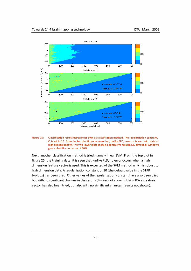
Towards 24-7 brain mapping technology DTU, March 2009
44
Figure 25: Classification results using linear SVM as classification method. The regularization constant, C, is set to 10. From the top plot it can be seen that, unlike FLD, no error is seen with data of high dimensionality. The two lower plots show no conclusive results, i.e. almost all windows give a classification error of 50%.
Next, another classification method is tried, namely linear SVM. From the top plot in
figure 25 (the training data) it is seen that, unlike FLD, no error occurs when a high
dimension feature vector is used. This is expected of the SVM method which is robust to
high dimension data. A regularization constant of 10 (the default value in the STPR
toolbox) has been used. Other values of the regularization constant have also been tried
but with no significant changes in the results (figures not shown). Using ICA as feature
vector has also been tried, but also with no significant changes (results not shown).
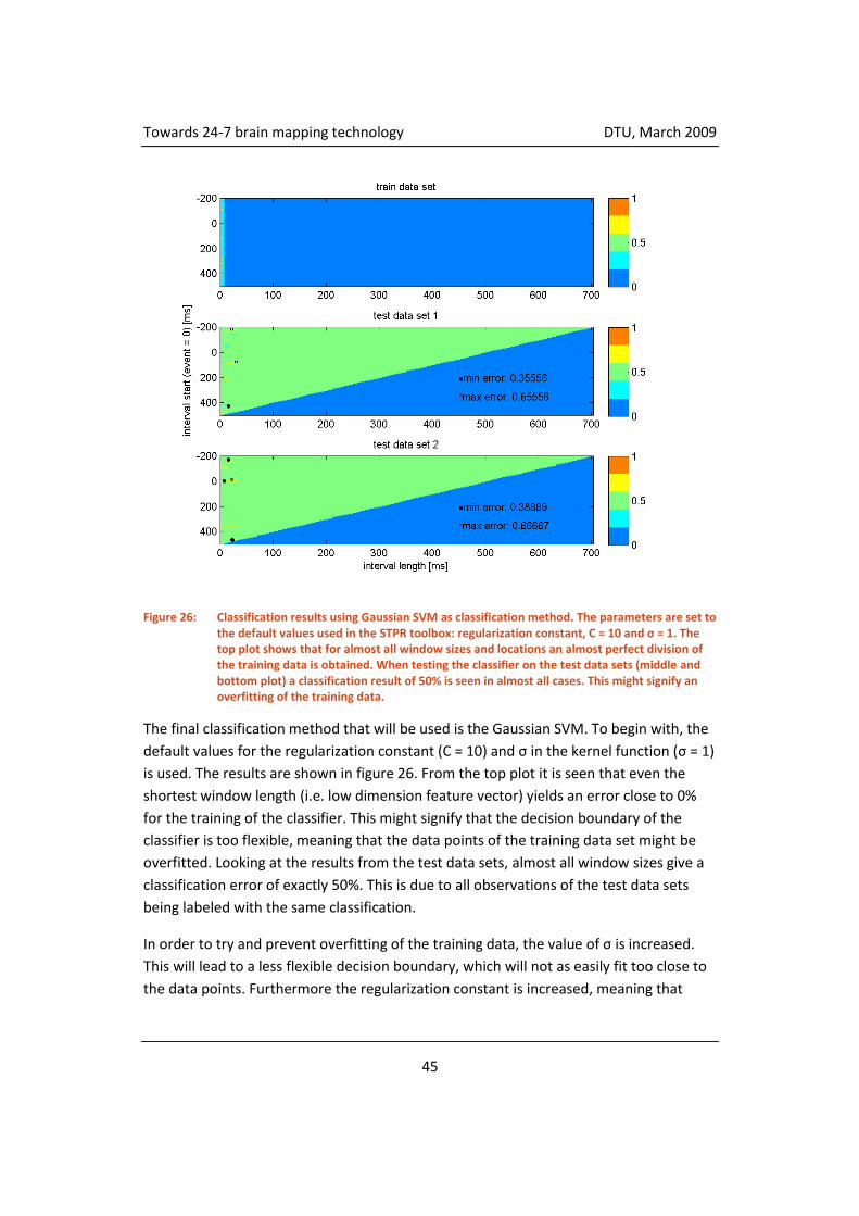
Towards 24-7 brain mapping technology DTU, March 2009
45
Figure 26: Classification results using Gaussian SVM as classification method. The parameters are set to the default values used in the STPR toolbox: regularization constant, C = 10 and σ = 1. The top plot shows that for almost all window sizes and locations an almost perfect division of the training data is obtained. When testing the classifier on the test data sets (middle and bottom plot) a classification result of 50% is seen in almost all cases. This might signify an overfitting of the training data.
The final classification method that will be used is the Gaussian SVM. To begin with, the
default values for the regularization constant (C = 10) and σ in the kernel function (σ = 1)
is used. The results are shown in figure 26. From the top plot it is seen that even the
shortest window length (i.e. low dimension feature vector) yields an error close to 0%
for the training of the classifier. This might signify that the decision boundary of the
classifier is too flexible, meaning that the data points of the training data set might be
overfitted. Looking at the results from the test data sets, almost all window sizes give a
classification error of exactly 50%. This is due to all observations of the test data sets
being labeled with the same classification.
In order to try and prevent overfitting of the training data, the value of σ is increased.
This will lead to a less flexible decision boundary, which will not as easily fit too close to
the data points. Furthermore the regularization constant is increased, meaning that

Towards 24-7 brain mapping technology DTU, March 2009
46
classification errors are penalized heavier. Figure 27 shows the results when using a
regularization constant of 75 and σ of 50. This combination of parameters was found to
give the most conclusive results. Looking at the results for test data set 1, a relatively
large area of classification error below 40% is seen, compared to the previous figures. In
this area is also seen the smallest classification error (31%) of all the tried classifications.
For test data set 2 a large fraction of the possible windows gives a classification error of
above 60%. Furthermore a maximum classification error of 73% is seen in this data set –
larger than any of the other tried classifications. The location of the area of high
classification error tells us that the data values from 150 ms to 350 ms after the event
might be the significant values for the classifier - although values before the event is also
necessary for giving good results.
In order to get a comparison value for the minimum and maximum errors, the exact
same run is made. The only difference is that the labels are randomly set before
calculating each point in the plot. In this random run a minimum classification error of
approximately 30% and a maximum error of 70% are found.
An example of the effect of changing the feature vector can be seen in figure 27. Looking
at the results for test data set 1 it can be seen that for a given set of electrodes and a
given classification method very different results are obtained. Using almost the same
start point of the window (150 ms), a change of the window length of only 40 ms
changes the classification accuracies from the minimum value of 31% to the maximum
value of 62%. This goes to show that just blindly selecting your feature vector might
produce seemingly random results.

Towards 24-7 brain mapping technology DTU, March 2009
47
Figure 27: Classification results using Gaussian SVM. Regularization constant is set to 75 and σ to 50. The middle plot (test data set 1) shows a low classification error for some different window sizes and placements. A classification error of 31% is the minimal found for test data set 1. For test data set 2 a high classification error (maximum 73%) is seen for many different window sizes and placements.
Using ICA as feature vector instead of the data values was also tried under the same
conditions used for figure 27. This was found to decrease the significance of the results.
For all the shown classifiers it was also tried to use other channels than the first
subcutaneous channel as well as using all four of the subcutaneous channels. This did
not improve the results, and in many cases worsened the results.
4.2.4 Conclusion on classification of visual stimuli
This section looks at the classification of a visual stimulus in the form of a checkerboard
changing color with a frequency of 2 Hz. The goal of the classification is to determine the
color of the top-left square of the checkerboard for the individual epochs. With the
paradigm of this test we are also armed with the knowledge that the checkerboard
changes to the other color with each observation. Therefore we can make our

Towards 24-7 brain mapping technology DTU, March 2009
48
conclusion of the checkerboard color based on all the observations from a given
segment.
From the literature it is known that a light flickering with a certain frequency gives a
signal in the visual cortex of the same frequency (Herrmann, 2001). Whether a 2 Hz
frequency can be found in the EEG signal is hard to determine due to the large amount
of noise in the low frequency ranges as seen on figure 19 – this has not been
investigated further.
Three different classification methods have been tried, i.e. FLD, linear SVM, and
Gaussian SVM. Classification with FLD and linear SVM did not produce any noteworthy
results.
The processed data values as well as the primary ICA component have been used as a
feature. Using the ICA component does not improve the results and in some cases
worsen the results compared to using the data values. This could be because the
important part of the data is contained in another component than the primary.
Regarding the location and length of the data values selected in the entire epoch, all
combinations were tried. This parameter was found to be very important for the
performance of the classifier.
The results shown in figure 27 (Gaussian SVM, C = 75, σ = 50) gives the most compelling
argument for whether this classification is possible or not. If a guess should be ventured
as to the conclusion of this classification exercise, it would be that the second segment
of showing the checkerboard starts with the same color as the first segment, and the
third segment of showing the checkerboard starts with the opposite color as the first
segment. But considering the amount of tests that have been tried, as well as the,
insignificant, maximal and minimal classification errors – 31% for test data set 1 and 73%
(equating to 27%) for test data set 2 - this result is not considered significant.

Towards 24-7 brain mapping technology DTU, March 2009
49
4.3 Classification of motor imagery tasks The foundation of this section is EEG data measured with a large number of electrodes.
The data is recorded from subjects performing two different cued motor imagery tasks.
Classification of these tasks into the two groups will be done. There are two main
purposes of this section:
1. To find ways to reduce the large amount of recorded data to a smaller feature vector
which more easily can be trained and tested. This will be done by applying various
methods for visualizing the content of the data.
2. To reduce the number of electrodes used in the classification. The large amount of
electrodes can be advantageous especially for investigative purposes, e.g. if you are
trying to locate an unknown dipole source. But the approach of this work is to learn
more about EEG for use in a BCI. In this regard a large number of electrodes is
inconvenient and should be avoided if possible. This section will thus focus on whether
the number of electrodes used can be reduced. A further advantage with reducing the
number of electrodes is that the computing time or hardware requirements for
calculation can be significantly reduced.
4.3.1 Description of dataset
The data was provided by Fraunhofer FIRST, Intelligent Data Analysis Group, and
Campus Benjamin Franklin of the Charité - University Medicine Berlin, Department of
Neurology, Neurophysics Group (Blankertz B. , 2004) . The data was provided for BCI
competition III, wherein participants try to achieve the best possible classification. The
aim of the experimental paradigm for this dataset (set IVa) was to discriminate trials of
different motor imagery tasks, based on a relatively small training set.
The subjects sat in a comfortable chair with arms resting on armrests. The subject does
not receive any form of feedback during the testing. Visual cues lasting 3.5 s were shown
on a computer screen. The cues indicated which of 3 motor imageries the subject should
perform: left hand, right hand, or right foot. Only trials for the classes of right hand, and
right foot are used in the analysis. Between the cues were relaxation periods of random
length (1.75 s to 2.25 s). Two different types of visual stimulation were used: either the
target cue on the screen was stationary or moving. 280 trials (140 hand trials, and 140
foot trials) are provided for each of five subjects. The 280 trials are divided into training
and test sets. In this analysis only one of the subjects (designated al) is used.
For the recording a 128 channel Ag/AgCl electrode cap was used. 118 EEG channels were
measured at positions established by the extended international 10/20 system as seen

Towards 24-7 brain mapping technology DTU, March 2009
50
on figure 28 (Oostenveld & Praamstra, 2001). The data was band-pass filtered between
0.05 and 200 Hz and digitized at 100 Hz with 0.1 μV accuracy.
Figure 28: Locations of electrodes in BCI competition data set IVa. 118 electrodes are shown labeled according to the extended international 10/20 system. Figure made in EEGLAB. The electrode system is described in (Oostenveld & Praamstra, 2001).
4.3.2 Preprocessing
The provided data is processed by the following steps:
1. The data is imported into EEGLAB.
2. For each channel the location was provided by a label, as per the extended
10/20 system. The label is translated to coordinates by EEGLAB on a head
model.
3. Unless otherwise noted, no filters (for cancelling noise) were used.
4. The data is divided into epochs according to the start of the visual cues. Each
epoch starts at -1 second and ends 3.5 seconds from the start of the cue.
5. Low frequency drifts and artifacts are removed by removing the mean baseline
(based on the pre-event interval) from each epoch individually.
6. No artifact rejection was run, in order to get results comparable with other
literature on this dataset.
4.3.3 Selection of electrodes
As described this data set contains recordings from 118 electrodes. In the paradigm used
in this experiment, we are looking for a response specifically in the sensorimotor cortex.

Towards 24-7 brain mapping technology DTU, March 2009
51
Thus, it might be possible to reduce the number of electrodes needed for the
classification.
As described in section 2.12.1 and section 2.6.2, specific areas of the sensorimotor
cortex show decreased activity when imagining a movement of specific body parts. For
instance imagining movement of the right hand leads to decreased power in the
contralateral sensorimotor cortex (left side), possibly in the area corresponding to the
electrode labeled C3. The decreased activity corresponding to the imagined foot
movement is located in the central area (possibly close to Cz).
Electrodes in the areas around C3 and Cz are considered likely candidates for the best
possible electrodes. This is also shown in (Wang, Gao, & Gao, 2005), where the authors
find that electrodes C3 and CPz are the best channels for calculating a feature based on
ERD, and Cz and FCz are best candidates for a ERP based feature. Based on prior
knowledge as well as the results from (Wang, Gao, & Gao, 2005) the following
electrodes are investigated in closer detail: The three central electrodes CPz, Cz, FCz, the
electrode above the motor cortex for the hand, C3, as well as the four electrodes closest
to C3: FCC3, C5, C1, and FCC3.
4.3.4 Extraction of features
In order to find features which can separate the two groups of trials, several
visualizations are used. In the visualizations the data is divided into the two groups:
Hand imagery and foot imagery. Although the classification needs to work on single trial
data, a look at plots averaged over all trials might give a good idea of which features are
useful. But one has to keep in mind that any discovered differences based on averaging
might not be useful as a feature for classification, since the variance might be so large as
to cause too many errors in the classification.
Figure 29 shows the ERP from the eight different channels. This is plotted in order to see
if a simple difference between ERP (see section 2.6.4) can be found in any of the
channels. As can be seen, all eight channels have some difference between hand and
foot imagery, but the most distinct difference is seen in channels Cz and FCz.
Interestingly a relatively much smaller difference between the two groups is seen in
electrode C3.
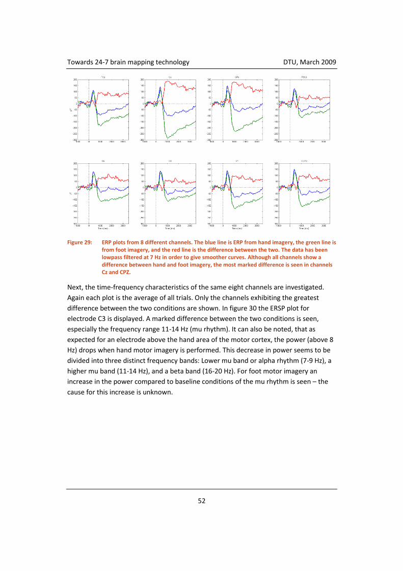
Towards 24-7 brain mapping technology DTU, March 2009
52
Figure 29: ERP plots from 8 different channels. The blue line is ERP from hand imagery, the green line is from foot imagery, and the red line is the difference between the two. The data has been lowpass filtered at 7 Hz in order to give smoother curves. Although all channels show a difference between hand and foot imagery, the most marked difference is seen in channels Cz and CPZ.
Next, the time-frequency characteristics of the same eight channels are investigated.
Again each plot is the average of all trials. Only the channels exhibiting the greatest
difference between the two conditions are shown. In figure 30 the ERSP plot for
electrode C3 is displayed. A marked difference between the two conditions is seen,
especially the frequency range 11-14 Hz (mu rhythm). It can also be noted, that as
expected for an electrode above the hand area of the motor cortex, the power (above 8
Hz) drops when hand motor imagery is performed. This decrease in power seems to be
divided into three distinct frequency bands: Lower mu band or alpha rhythm (7-9 Hz), a
higher mu band (11-14 Hz), and a beta band (16-20 Hz). For foot motor imagery an
increase in the power compared to baseline conditions of the mu rhythm is seen – the
cause for this increase is unknown.

Towards 24-7 brain mapping technology DTU, March 2009
53
Figure 30: ERSP plot for electrode C3 located over the hand motor cortex (see description of this type of plot in section 3.2.2). Condition 1 is hand motor imagery and condition 2 is foot motor imagery. The panel to the right shows condition 1 minus condition 2. A significant difference is seen in the frequency range 11-14 Hz starting at 1000 ms. The difference is caused by a decrease of power (ERD) in the hand motor imagery tasks as well as an increase in power (ERS) during the foot motor imagery tasks.
Figure 31 and figure 32 displays the ERSP plot for the centrally located electrodes Cz
respectively CPz. A significant difference is seen in the beta band, but at a higher
frequency (19-24 Hz) than was seen in the C3 electrode (16-20 Hz). As expected the
trials for the foot motor imagery show a decrease in power in this higher beta band
shortly after the event (400 ms to 1400 ms). Another detail to take note of in these
figures is the early low frequency component (0-3 Hz, 400-1000 ms). This corroborates
the ERP findings seen in figure 29. The greater difference between hand and foot motor
imageries in electrode Cz and CPz compared to C3, is also reflected in these plots: the
low frequency component is less pronounced in electrode C3.
When looking at the foot imagery conditions for the electrodes that supposedly are
positioned close to the foot motor cortex, no significant ERD is seen in the mu band as
would be expected for a motor imagery. Only electrode CPz shows any kind of
desynchronization in this band, but the desynchronization is seen for both conditions
with no significant difference between the two.
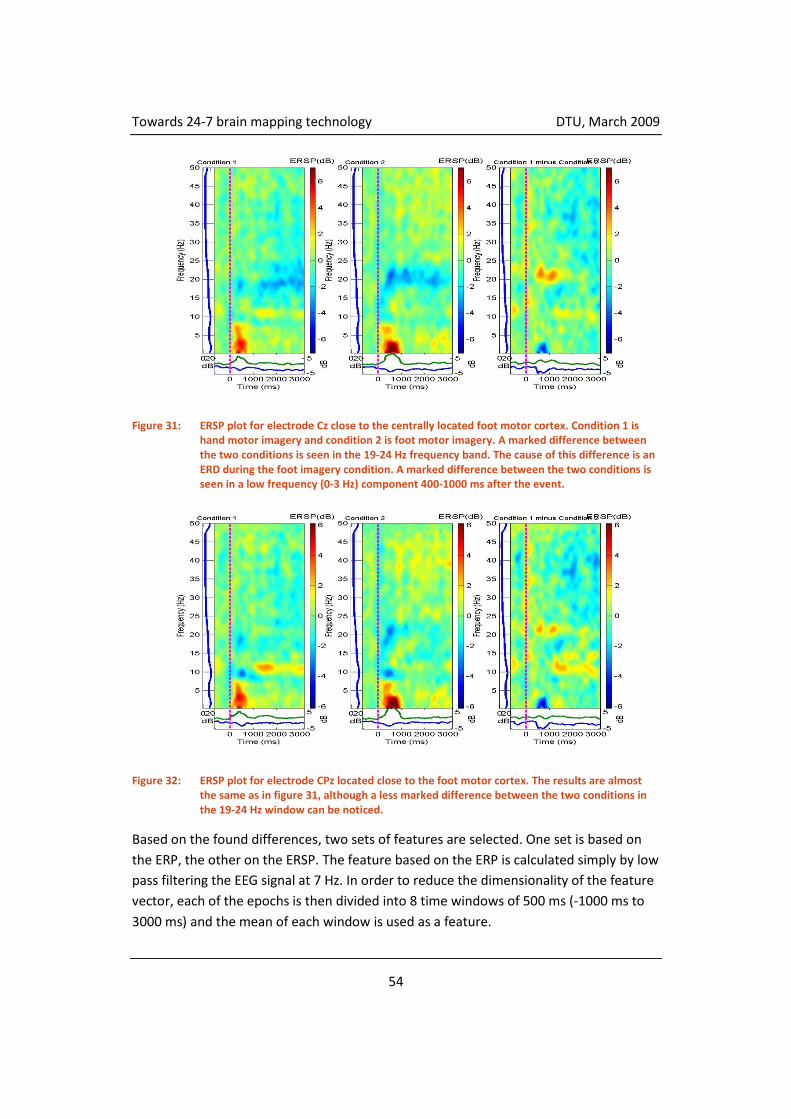
Towards 24-7 brain mapping technology DTU, March 2009
54
Figure 31: ERSP plot for electrode Cz close to the centrally located foot motor cortex. Condition 1 is hand motor imagery and condition 2 is foot motor imagery. A marked difference between the two conditions is seen in the 19-24 Hz frequency band. The cause of this difference is an ERD during the foot imagery condition. A marked difference between the two conditions is seen in a low frequency (0-3 Hz) component 400-1000 ms after the event.
Figure 32: ERSP plot for electrode CPz located close to the foot motor cortex. The results are almost the same as in figure 31, although a less marked difference between the two conditions in the 19-24 Hz window can be noticed.
Based on the found differences, two sets of features are selected. One set is based on
the ERP, the other on the ERSP. The feature based on the ERP is calculated simply by low
pass filtering the EEG signal at 7 Hz. In order to reduce the dimensionality of the feature
vector, each of the epochs is then divided into 8 time windows of 500 ms (-1000 ms to
3000 ms) and the mean of each window is used as a feature.

Towards 24-7 brain mapping technology DTU, March 2009
55
The same time windowing is used for the ERSP based feature. Two different frequency
windows are selected: One at 11-14 Hz and another at 19-24 Hz. The mean of each of
the two-dimensional windows (combination of time window and frequency window) is
found and used as a feature.
If both feature types are used each channel provides 24 features.
4.3.5 Classification
The two groups of features described in the previous section can now be applied to a
classifier. Three different classifiers have been tested, namely Fisher’s linear
discriminant, linear SVM, and Gaussian SVM. The regularization parameter of both the
linear SVM and Gaussian SVM has been set to 104, and σ for the Gaussian SVM has also
been set to 104. These parameters were found to yield the best results in this case.
The classification accuracy has been determined by leave-one-out crossvalidation.
The results of the classifications are seen in table 2 using different combination of
features (ERP, ERSP, or both) and different combination of channels for which the
features have been calculated.
Different channel combination has been tried:
1) All 118 electrodes
2) CPz, Cz, FCz, C3, FCC3, C5, C1, CCP3
3) C5, C3, C1, Cz
4) FCz, Cz, CPz for ERP and C3, Cz, CPz for ERSP
Combination 1 is chosen in order to see how the classification algorithms handle feature
vectors of relatively high dimension. Combination 2 is the eight electrodes described
earlier. Combination 3 consists of four electrodes located in a straight line from the ear
to the top of the head. This combination is chosen to simulate the location of electrodes
that might be obtained by a device such as Hypo-Safe’s. Combination 4 is the electrodes
found to give the best classification accuracy with the FLD classifier.
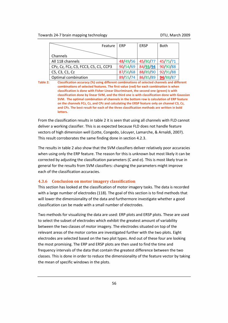
Towards 24-7 brain mapping technology DTU, March 2009
56
Feature Channels
ERP ERSP Both
All 118 channels 48/49/56 45/80/77 45/75/71
CPz, Cz, FCz, C3, FCC3, C5, C1, CCP3 90/54/69 84/93/94 90/90/88
C5, C3, C1, Cz 87/50/68 88/89/90 92/91/88
Optimal combination 89/55/74 86/85/89 94/88/87 Table 2: Classification accuracy (%) using different combinations of selected channels and different
combinations of selected features. The first value (red) for each combination is when classification is done with Fisher Linear Discriminant, the second one (green) is with classification done by linear SVM, and the third one is with classification done with Gaussian SVM. The optimal combination of channels in the bottom row is calculation of ERP feature on the channels FCz, Cz, and CPz and calculating the ERSP feature only on channel C3, Cz, and CPz. The best result for each of the three classification methods are written in bold letters.
From the classification results in table 2 it is seen that using all channels with FLD cannot
deliver a working classifier. This is as expected because FLD does not handle feature
vectors of high dimension well (Lotte, Congedo, Lécuyer, Lamarche, & Arnaldi, 2007).
This result corroborates the same finding done in section 4.2.3.
The results in table 2 also show that the SVM classifiers deliver relatively poor accuracies
when using only the ERP feature. The reason for this is unknown but most likely it can be
corrected by adjusting the classification parameters (C and σ). This is most likely true in
general for the results from SVM classifiers: changing the parameters might improve
each of the classification accuracies.
4.3.6 Conclusion on motor imagery classification
This section has looked at the classification of motor imagery tasks. The data is recorded
with a large number of electrodes (118). The goal of this section is to find methods that
will lower the dimensionality of the data and furthermore investigate whether a good
classification can be made with a small number of electrodes.
Two methods for visualizing the data are used: ERP plots and ERSP plots. These are used
to select the subset of electrodes which exhibit the greatest amount of variability
between the two classes of motor imagery. The electrodes situated on top of the
relevant areas of the motor cortex are investigated further with the two plots. Eight
electrodes are selected based on the two plot types. And out of these four are looking
the most promising. The ERP and ERSP plots are then used to find the time and
frequency intervals of the data that contain the greatest difference between the two
classes. This is done in order to reduce the dimensionality of the feature vector by taking
the mean of specific windows in the plots.

Towards 24-7 brain mapping technology DTU, March 2009
57
Although the chosen method of reducing the feature vector was not compared with any
other method, it seems to provide a reasonable accuracy of classification. A secondary
benefit of reducing the size of the feature vector is that the training and testing of the
classifier can be performed with considerable less computing power.
The best classification accuracy achieved is 94% accuracy. This same result was obtained
by either Gaussian SVM classification using only the ERSP feature with 8 channels, or by
FLD classification using both features on only 3 channels per feature group (4 unique
channels).
The achieved accuracy can be compared with results from the BCI competition
(Blankertz B. , 2004). In the competition there is data from five subjects but only one of
the subjects has been used in this work. Furthermore LOO cross-validation has been
used in this work and not in the competition results, making the results not directly
comparable. If only looking at the same subject as was used in this section, the 14
participants in the competition achieved accuracies between 53.6% and 100%. The
obtained accuracy of 94% would equate to a 7th-9th place.
All in all this section proved that it is possible to reduce the number of electrodes to 4
while still maintaining a classification accuracy of at least 94%. If an additional constraint
is put on the selection of electrodes – that they must be on a straight line on the scalp–
a classification accuracy of 92% is achieved. This constraint is to simulate the limitations
Hypo-Safe’s device has in electrode placement. By carefully selecting the features these
classifications can be done by the fast classification algorithm FLD.

Towards 24-7 brain mapping technology DTU, March 2009
58
5 Discussion As described in the introduction, the focus of this study is to examine the possible
problems and limits of using a device like the one Hypo-Safe is developing at the
moment. Two main areas have been considered: the validity of the data recorded with
subcutaneous electrodes and the limits encountered in classification of data by using
only a few electrodes.
5.1 Validity of data from subcutaneous electrodes In section 4.1 the data recorded from subcutaneous electrodes is examined in
comparison with data recorded simultaneously from ordinary surface electrodes. Only a
limited amount of data is available, making any conclusion of this comparison uncertain.
An additional factor that possibly reduces the certainty of the conclusion is the following
issue: The subcutaneous electrode used in the experiment was inserted under the skin
and the wire attached to ordinary EEG recording equipment. Consequently, one might
imagine that the presence of an open puncture wound might influence the collection of
the data. Oozing blood around the wound might cause artifacts and give a poor
electrode contact. The subcutaneous electrode closest to the puncture site was found to
yield the poorest results. This can maybe corroborate the theory that oozing blood
causes artifacts or poor electrode contact. The oozing blood will not be present if both
electrode and recording device is implanted, and the skin has healed tightly around the
electrode.
As concluded in section 4.1.7 the data obtained from subcutaneous electrodes is very
similar to the data obtained from surface electrodes. But a number of small differences
between the subcutaneous and surface electrodes are seen (more artifacts, less noise,
and higher amplitude in the subcutaneous electrodes). Considering the small amount of
data as well as the lack of confidence for the results, these differences are not significant
enough to conclude whether the small differences seen speak in favor of the
subcutaneous electrodes or the surface electrodes.
5.2 Limits in classification performance using few electrodes In section 4.2 a classification of VEP events using between 1 and 4 electrodes is
performed. Section 4.3 describes a classification of motor imagery events using data
from between 4 and 118 electrodes.
The classifiers found in section 4.2 cannot predict the data with the few closely spaced
subcutaneous electrodes. But the reason that the classification did not yield conclusive
results is not known. It can be due to the electrodes not being placed in the area of the

Towards 24-7 brain mapping technology DTU, March 2009
59
brain responsible for the needed signal; it can be because the effect is simply not
measurable with EEG at all; or perhaps that more than the few electrodes supplied are
needed in order to record the differences.
The results from section 4.3 show that if the features and electrodes are chosen
carefully FLD produces very good results. SVM has the advantage that you can take any
combination of electrodes and get a reasonable classification without optimization.
These results also show that even when reducing the number of electrodes from 118 to
4 a good classification is still obtainable. Even though it is shown that few electrodes is
enough to get a good classification, this result is not directly comparable with the
recordings that will be made with Hypo-Safe’s device. The spatial distribution of the
subcutaneous electrodes in the device is much tighter than the spatial distribution of the
four electrodes in the motor imagery classification.
The tight spatial distribution can perhaps prove to be a problem if the device is to be
used for other purposes such as a BCI system. One way to solve this would be to attach a
longer electrode to the device if possible. Another way to solve the problem of close
spatial distribution would be to select other motor imageries than hand and foot.
Tongue and lips are an example of a pair of motor imageries that are closer together on
the motor cortex as shown in figure 3 on page 7.
5.3 Improvements This section suggests various improvements that can be made to the analysis performed
in section 4.
Comparison of the subcutaneous and surface electrodes by looking at the
countinous data: Further knowledge about the subcutaneous electrodes migh
be obtained by employing comparison methods usable on the continuous data.
This would allow one to look at all the data and not just the epoched data. An
example of such a method is scatter plots which can compare the data values of
each electrode with the other electrodes. This can be done using the plotmatrix
function from matlab.
ERSP plots for VEP classification: The classification of the VEP trials is only
performed with the data values as feature vector. Perhaps investigating for
specific time-frequency differences between the two classes might provide new
information.
PCA before FLD: In a few cases the FLD classification gave poor results due to the
dimensionality of the feature vector being too high. This might be alleviated by
reducing the dimensionality with for instance PCA or ICA beforehand.

Towards 24-7 brain mapping technology DTU, March 2009
60
Examination of the weight vector: One way to examine the importance of the
individual features in the feature vector, would be to look at the weight vector
of the classifier and remove features that are less important.
Artifact rejection combined with classification: You might obtain better results
by investigating epochs with an artifact rejection method before classifying. The
individual trials could be labeled with a measure of the certainty of it being an
artifactual epoch. This would allow a further investigation of trials which have
been classified with the wrong label.
5.4 Perspective It seems possible that Hypo-Safe’s device might be usable as the foundation of a BCI
system as well as many other applications. Some problems still exist though. Further
research into the limits of the low spatial resolution of the electrodes is needed. In
relation to this a good control input to such a BCI system needs to be found. A more
practical issue is with the calibration of the BCI system. When establishing a BCI long
calibration sessions are usually needed in order to find the specific features in the data
that gives the best classification for a given subject. If a BCI system is to be put into
widespread clinical use, this is a problem that needs to be addressed. The generalized
methods for feature selection used in this work, e.g. ERSP plots, might be advantageous
for selecting exactly the best feature for a given subject. The selection of features based
on such a measure can be (semi)automated. Recently, work has been done into the
reduction of the time needed for the calibration session by using well established
knowledge of the EEG changes in response to the function used to control the BCI
(Blankertz, Dornhege, Krauledat, Müller, & Curio, 2007). Use of prior knowledge
combined with an automated system might improve the time needed for calibration of a
BCI system.

Towards 24-7 brain mapping technology DTU, March 2009
61
6 Conclusion This section sums up the conclusions from each of the three data analysis sections.
Further details about the conclusions can be seen in the sections 4.1.7, 4.2.4, and 4.3.6
on pages 38, 47, respectively 56.
The use of closely spaced subcutaneously implanted electrodes for EEG recording is
examined.
A comparison between conventional electrodes and subcutaneous electrodes is made.
Only a limited amount of data material is available. Several methods are employed for
the comparison: frequency spectra, ERP, the amount of artifacts, and ICA
decomposition. The analysis shows that the data recorded from the two different
recording methods is almost identical, although some differences are found. The found
differences do not give a clear picture of whether the subcutaneous electrodes provide
better or worse data compared to the conventional electrodes.
A classification of two different data sets is done in order to investigate the use of a
limited amount of electrodes: 1) Classification of a data set containing visual evoked
potential (VEP) trials is performed by three different classification methods: Fisher’s
linear discriminant (FLD), linear support vector machines (SVM), and Gaussian SVM. A
good classification from the supplied data is not possible. 2) Classification of a data set
containing tasks based on motor imagery is performed. FLD, linear SVM, and Gaussian
SVM are used as classifiers. Feature extraction is performed on the basis of event
related potential (ERP) and event related spectral perturbation (ERSP). Using only four
electrodes a classification accuracy of 94% is obtained. The results from the second
classification show that it is possible to perform a successful classification using only a
few electrodes.

Towards 24-7 brain mapping technology DTU, March 2009
62
7 References Aurlien, H. (2004). EEG background activity described by a large computerized database.
Clinical Neurophysiology , 115 (3), 665-673.
Bell, A. J., & Sejnowski, T. J. (1995). An information-maximization approach to blind
separation and blind deconvolution. Neural Comput , 7 (6), 1129-1159.
Blankertz, B. (2004, 12 12). BCI Competition III. Retrieved 02 25, 2009, from BCI
Competition III: http://ida.first.fraunhofer.de/projects/bci/competition_iii/
Blankertz, B., Dornhege, G., Krauledat, M., Müller, K. R., & Curio, G. (2007). The non-
invasive Berlin Brain-Computer Interface: fast acquisition of effective performance in
untrained subjects. NeuroImage , 37 (2), 539-550.
Cotterill, R. (1998). Enchanted Looms: Conscious Networks in Brains and Computers.
Cambridge University Press.
Delorme, A., & Makeig, S. (2004). EEGLAB: an open source toolbox for analysis of single-
trial EEG dynamics including independent component analysis. J Neurosci Methods , 134
(1), 9-21.
Dubuc, B. (2009, 03 15). The Motor Cortex: The Brain From Top to Bottom. Retrieved 03
15, 2009, from The Brain From Top to Bottom: http://thebrain.mcgill.ca/
Emotiv Systems. (2009, 03 02). Retrieved 03 02, 2009, from Emotiv Systems:
http://emotiv.com/
Fabiani, M., Gratton, G., & Coles, M. G. (2000). Event-related brain potentials - methods,
theory, and applications. (J. T. Cacioppo, L. G. Tassinary, & G. G. Bertson, Eds.)
Cambridge: University Press.
Franc, V., & Hlavac, V. (2008, 08 15). Statistical Pattern REcognition Toolbox for Matlab
v. 2.09. Retrieved 12 03, 2008, from Statistical Pattern REcognition Toolbox for Matlab:
http://cmp.felk.cvut.cz/cmp/software/stprtool/
Herrmann, C. S. (2001). Human EEG responses to 1-100 Hz flicker: resonance
phenomena in visual cortex and their potential correlation to cognitive phenomena.
Experimental Brain Research , 137 (3), 346-353.
Hypo-Safe. (2009, 02 23). Retrieved 02 23, 2009, from Hypo-Safe:
http://www.hyposafe.com

Towards 24-7 brain mapping technology DTU, March 2009
63
Kamphuisen, H. A., Dulken, H., Janssen, A. J., Huyser, W. W., Sweden, B., Kemp, B., et al.
(1991). Sleep-Wake Recording of Forty Day Duration Using Subcutaneous Electrodes.
Epilepsia , 32 (3), 347-350.
Lee, T.-W., & Sejnowski, T. J. (1998). Independent component analysis for mixed
subgaussian and super-gaussian sources. Technical report, Computational Neurobiology
Lab, The Salk Institute, La Jolla .
Lotte, F., Congedo, M., Lécuyer, A., Lamarche, F., & Arnaldi, B. (2007). A review of
classification algorithms for EEG-based brain-computer interfaces. J. Neural Eng. , 4 (2),
1.
Lunts, A., & Brailovskiy, V. (1967). Evaluation of attributes obtained in statistical decision
rules. Engineering Cybernetics , 3, 98-109.
Makeig, S. (1993). Auditory event-related dynamics of the EEG spectrum and effects of
exposure to tones. Electroencephalography and clinical neurophysiology , 86 (4), 283-
293.
Makeig, S., Bell, A. J., Jung, T.-P., & Sejnowski, T. J. (1996). Independent component
analysis of electroencephalographic data. in Advances in Neural Information Processing
Systems, 8, pp. 145-151.
Markram, H. (2009, 03 15). Gallery: Blue Brain Project. Retrieved 03 15, 2009, from Blue
Brain Project: http://bluebrain.epfl.ch/
Megias, M., Emri, Z., Freund, T. F., & Gulyas, A. I. (2001). Total number and distribution
of inhibitory and excitatory synapses on hippocampal CA1 pyramidal cells. Neuroscience
, 102 (3), 527-540.
Nunez, P. L. (2005). Electric Fields of the Brain: The Neurophysics of Eeg. Oxford Univ Pr
(Txt).
Nuwer, M. R., Comi, G., Emerson, R., Fuglsang-Frederiksen, A., Guerit, J.-M., Hinrichs, H.,
et al. (1998). IFCN standards for digital recording of clinical EEG. Electroencephalography
and Clinical Neurophysiology , 106 (3), 259-261.
Odom, J. V., Bach, M., Barber, C., Brigell, M., Marmor, M. F., Tormene, A. P., et al.
(2004). Visual evoked potentials standard (2004). Documenta ophthalmologica.
Advances in ophthalmology , 108 (2), 115-123.

Towards 24-7 brain mapping technology DTU, March 2009
64
Oostenveld, R., & Praamstra, P. (2001). The five percent electrode system for high-
resolution EEG and ERP measurements. Clinical neurophysiology : official journal of the
International Federation of Clinical Neurophysiology , 112 (4), 713-719.
Pfurtscheller, G., & Lopes da Silva, F. H. (1999, November). Event-related eeg/meg
synchronization and desynchronization: basic principles. Clin Neurophysiol , 110 (11), pp.
1842-1857.
Pfurtscheller, G., Brunner, C., Schlogl, A., & Lopesdasilva, F. (2006). Mu rhythm
(de)synchronization and EEG single-trial classification of different motor imagery tasks.
NeuroImage , 31 (1), 153-159.
Srinivasan, R., Winter, W. R., Ding, J., & Nunez, P. L. (2007). EEG and MEG coherence:
Measures of functional connectivity at distinct spatial scales of neocortical dynamics. J
Neurosci Methods , 166 (1), 41-52.
University of Colorado at Boulder. (2009, 03 15). Functional organization of the brain.
Retrieved from University of Colorado at Boulder - Department of Integrative
Physiology: http://www.colorado.edu/intphys/
Wang, Y., Gao, S., & Gao, X. (2005). Common Spatial Pattern Method for Channel
Selelction in Motor Imagery Based Brain-computer Interface. Conference proceedings :
... Annual International Conference of the IEEE Engineering in Medicine and Biology
Society. IEEE Engineering in Medicine and Biology Society. Conference , 5, 5392-5395.
Wikipedia - Electroencephalography. (2009, 03 10). Retrieved 03 10, 2009, from
Wikipedia: http://en.wikipedia.org/wiki/Electroencephalography
Wikipedia - Linear discriminant analysis. (2009, februar 23). Retrieved from Wikipedia:
http://en.wikipedia.org/wiki/Linear_discriminant_analysis
Wikipedia - Support vector machine. (2009, 02 25). Retrieved from Wikipedia:
http://en.wikipedia.org/wiki/Support_vector_machine
Wurtz, R. H., & Kandel, E. R. (2000). Central Visual Pathways (Fourth ed.). (E. R. Kandel, J.
H. Schwartz, & T. M. Jessell, Eds.) New York: McGraw-Hill.


