Tourism and Economic Development:

Evidence from Mexico’s Coastline∗

Benjamin Faber†and Cecile Gaubert‡

September 2015– Preliminary and Incomplete –

Abstract

Tourism is one of the most visible and fastest growing facets of globalization in developingcountries. Despite widespread policy interest, however, we currently have limited empiricalevidence on the economic consequences of this channel of market integration. This paper com-bines a quantitative spatial equilibrium model of trade in goods and tourism services with arich collection of Mexican microdata and a new empirical strategy to estimate the long-runeconomic consequences of tourism. We begin by using the data to estimate a number of re-duced form effects of tourism on local economic outcomes in today’s cross-section of Mexi-can municipalities. To base these estimations on plausibly exogenous variation in long-termtourism exposure, we exploit geological and oceanographic variation in beach quality alongthe Mexican coastline, and use historical high-resolution satellite data to construct instrumen-tal variables. To guide the estimation of tourism’s welfare implications, we then write downa spatial equilibrium model, and use the reduced form moments to inform its calibration forcounterfactual analysis. We find that tourism causes large and significant increases in long runlocal real economic activity. Contrary to much of the existing literature on tourism and de-velopment, these effects are driven by sizable positive spillovers on traded goods production.In the aggregate, however, we find that these spillovers are largely offset by reductions in ag-glomeration economies among non-touristic regions, so that the national gains from tourismare mainly driven by a classical market integration effect. Finally, we find that the distributionof these gains significantly differs across groups of gender, education, ethnicity and age, andquantify the interplay of forces that underlie this heterogeneity.

Keywords: Tourism, economic development, spatial equilibrium, gains from trade.JEL Classification: F15, F63, O24.

∗Nicholas Li and Jose Vasquez-Carvajal provided excellent research assistance. We thank Andrés Rodríguez-Clareand participants at multiple conferences/seminars for helpful comments.†Department of Economics, UC Berkeley and NBER.‡Department of Economics, UC Berkeley.

1 IntroductionTourism is a peculiar form of market integration. Instead of shipping goods across space,

tourism involves the export of non-traded local amenities, such as beaches, mountains or cul-tural amenities, and local services, such as hotels, restaurants and local transport, by temporarilymoving consumers across space. Tourist expenditures on these local services are then reported astourism exports in cross-country data on services trade flows. Over recent decades these tourismexports have grown to become a quantitatively important channel of global integration, and thisis particularly the case for developing countries.1

Unsurprisingly in this context, tourism has attracted widespread policy attention in both de-veloped and developing countries. Virtually every country in the world has one or several pub-licly funded tourism promotion agencies. Some governments and international organizationshave also been advocating the promotion of tourism to foster local economic development ineconomically lagging regions within countries.2 On the other hand, much of the existing socialsciences literature on tourism has been critical about its long run economic consequences, espe-cially in developing countries.3 For example, Honey (1999) and Dieke (2000) have questionedthe extent to which the gains from tourism accrue to the local population, rather than being cap-tured by multinationals or domestic elites. In economics, the existing literature has argued thattourism may give rise to a particular form of the "Dutch disease" by reallocating factors of produc-tion towards stagnant services activities and away from traded sectors with higher potential forproductivity growth (Copeland, 1991).

Despite the rapid growth of tourism and widespread policy attention, the existing literatureon trade and development has so far paid relatively little attention to this channel of market in-tegration. This paper aims to fill this gap. The analysis makes two main contributions. First,we combine a rich collection of Mexican microdata with a new empirical strategy to estimate anumber of reduced form effects of tourism on local economic outcomes. To base estimations onplausibly exogenous variation in long term tourism exposure in today’s cross-section of Mexicanmunicipalities, we propose an instrumental variable (IV) strategy that exploits historical high-resolution satellite data on geological and oceanographic variation in beach quality along theMexican coastline. Second, we write down a quantitative spatial equilibrium model of trade ingoods and tourism services, and use the estimated reduced form empirical moments to inform itscalibration. The model allows us to quantify the welfare implications of tourism in Mexico and thedistribution of the gains from tourism across different groups of the Mexican society. It also shedslight on the underlying channels. For instance, the model explicitly allows for potentially adverse

1World tourism exports were USD 1.25 trillion in 2014, making it the single largest sector of global trade in services.Tourism exports of low and middle income countries have grown at an average annual rate of 11 percent over theperiod 1982-2012. For this group of countries, tourism exports have been of the same magnitude as 75 percent of allfood and agriculture exports combined, and 60 percent of total FDI inflows over the past decade. Figures are based onUNCTAD statistics (see http://unctad.org/en/pages/Statistics.aspx).

2See for example "Passport to Development" (WorldBank, 1979) or "Tourism and Poverty Alleviation: Untapped Potential"(DFID, 1999).

3See Hawkins & Mann (2007) for a review of this literature.

1

effects of tourism by introducing different sources of local production externalities. By altering thescale of local production, tourism can affect the productivity of traded goods production. Thesespillover effects operate in addition to the standard general equilibrium effects through wagesand prices. Depending on the sign and size of the within and cross-sector spillovers, the aggre-gate gains from tourism can either be magnified or diminished compared to the conventionalgains from market integration in tourism.

At the center of the analysis lies the construction of a rich collection of microdata. We as-semble a database containing: i) municipality-level hotel revenues, employment, population andwages by gender, education, age and ethnicity, and output by sector from the Mexican CensosEconomicos in 1998 and 2008 and the Mexican population censuses in 2000 and 2010; ii) a longtime series of census data for consistent spatial units covering the period 1921-2010; iii) remotesensing satellite data at a resolution of 30x30 meter pixels covering roughly 9,500 km of Mexicancoastline across six different bands of wavelength during the 1980s and 90s; iv) a vector of local(dis-)amenities including restaurant and store density, road accidents, environmental pollutionand crime collected from several administrative sources; v) municipality-level public finance datacovering the period 1989-2010; and vi) panel data on bilateral tourism exports and relative pricescovering 115 countries over the period 1990-2011.

Armed with this database, the analysis proceeds in four main steps. In step 1, we estimatea number of motivating reduced from effects of tourism on municipality-level population, em-ployment, and wages by groups of gender, education and ethnicity, and local GDP by sector ofactivity. We take inspiration from the tourism management literature that has argued that tourismactivity can to a large extent be determined by the quality of a very specific set of local naturalcharacteristics (e.g. Weaver et al. (2000)). We identify a set of beach quality criteria from thatliterature (Leatherman, 1997), such as the presence of a nearby offshore island or the fraction ofonshore coastline covered by white sand beaches, and use our satellite data to construct a numberof instrumental variables capturing tourism attractiveness along the Mexican coastline.

The identifying assumption is that islands or the fraction of coastline covered by picture-perfect sand beaches do not affect local economic outcomes in today’s cross-section of Mexicanmunicipalities relative to other coastal municipalities except through their effect on tourism activ-ity. We assess the validity of this assumption in several ways. We report how OLS and IV pointestimates are affected by the inclusion of observable pre-determined municipality controls, andassess whether six different instrumental variables yield similar point estimates. To further assessthe extent to which the IVs may impact the local economy by directly affecting the amenities oflocal residents or being correlated with natural advantages in other sectors, we also construct along time series of population census data for consistent spatial units in Mexico, and estimate theeffect of the IVs on municipality populations in periods before beach tourism became a major forcein Mexico (censuses of 1921, 1930, 1940 and 1950) as a placebo falsification test. Finally, we alsoverify the extent to which our IVs are correlated with model-based estimates of local amenities intoday’s cross-section of municipalities.

Using this empirical strategy, we find that variation in local tourism activity has strong and

2

significant long-term positive effects on municipality total employment, population, local GDPand wages. According to our preferred specification, a one standard deviation increase in localtourism expenditure in today’s cross-section of Mexican municipalities leads to a doubling of mu-nicipality total employment, and increases nominal municipality GDP by a factor of 2.5. Theseeffects appear to be driven by sizable multiplier effects on other local sectors of activity. For ex-ample, a one standard deviation increase in local tourism expenditure more than doubles localmanufacturing GDP. Importantly, these effects do not appear to be sensitive to excluding tourismcenters that were planned and subsidized by the government or to taking into account differencesin public investments across touristic and non-touristic places. The data also allow us to break upthe effects on employment, population and wages by different groups of the Mexican society. Wefind that the employment gains are biggest in proportional terms for skilled relative to unskilledlabor, for women relative to men, and for indigenous workers relative to Hispanic workers.

In step 2, we interpret these results through the lens of a quantitative multi-country multi-region spatial equilibrium model. To this end, we extend the theoretical framework of Redding(2015). The model features trade in tourism services in addition to trade in goods. Falling cross-border or within-country frictions to tourism give rise to gains from a classic market integrationeffect, and these gains may be unequally distributed across different groups of the population. Ontop of that effect, we allow tourism to affect welfare through local production externalities. In themodel, tourism affects the economic activity of traded sectors (manufacturing) through two chan-nels. First, it affects other sectors through its general effect on wages and prices. For example, apositive shock on tourism pushes local wages up, which may decrease local manufacturing activ-ity. Second, it affects the local scale of economic activity in services production and traded goodsproduction which may impact manufacturing productivity through local within and cross-sectorproductivity spillovers.

In step 3, we use the data to estimate the key parameters of the model, and calibrate it tocurrent-day Mexico as a reference equilibrium. We first estimate the elasticity of substitution be-tween different touristic destinations (the trade elasticity for trade in tourism services). To doso, we use bilateral country-level panel data on tourism exports, and use nominal exchange ratechanges to instrument for relative local consumption prices across different destinations. We thenestimate the spatial labor supply elasticity. To do so, we exploit the identifying assumption thatour IVs affect local employment and population only through their effect on local real wages. Fi-nally, to inform the calibration of the sign and size of tourism’s spillover effects, we use the struc-ture of the model to compute a counterfactual equilibrium with prohibitive frictions to tourism.We then calibrate the spillovers such that the outcomes of the counterfactual equilibrium can repli-cate the placebo regressions ran in the empirical exercise on historical data.

In step 4, armed with these parameters and a number of observed moments in our data, weproceed to explore model-based counterfactuals. We solve for the welfare implications of mov-ing from the current levels of domestic and international tourism to a prohibitive level of tourismfrictions. This allows us to quantify the aggregate welfare gains from tourism, decompose thesegains into different channels, and analyze the extent to which the gains from tourism are unequally

3

shared across different groups of the population.We find that tourism causes significant gains to the average Mexican household that are in the

order of 2.9 percent of household incomes nationally. These gains are driven by an interestinginterplay of channels. Contrary to much of the existing literature on tourism and economic devel-opment, we find that tourism leads to sizable positive spillovers on local traded goods productionthat operate in addition to a classical market integration effect. We estimate that this spillover ef-fect is due to both a significant cross-sector externality between services production and manufac-turing as well as within-sector localization economies in manufacturing. While these two sourcesof agglomeration economies reinforce one another leading to large observed reallocations of man-ufacturing production and total GDP towards tourism centers, we find that they largely offset oneanother for the aggregate national implications of tourism. That is, while tourism leads to largelocal gains in agglomeration economies for traded goods production, these gains are largely off-set by reductions in agglomeration economies among non-touristic regions, so that the aggregategains from tourism are mainly driven by a classical market integration effect.

Finally, we use the data and our model to explore the heterogeneity of the gains from tourismacross different groups of the Mexican society. We find that while the gains are on average posi-tive and significant for all groups, they are also significantly regressive when taking into accountthe pre-existing distribution of nominal incomes across these groups. Analyzing the underlyingchannels, we find that the majority of the estimated heterogeneity is due to differences in tourism’sfactor intensities across different types of labor, which operate in addition to differences in spatialmobility and in evaluations of tourism’s effect on local amenities.

This paper contributes to the recent literature on trade and development (e.g. Topalova (2010),Donaldson (in press), Atkin et al. (2015)). Relative to the existing literature, this paper sets focuson tourism, an important and fast-growing but somewhat overlooked facet of globalization in de-veloping countries. There is a small existing empirical literature that has analyzed cross-countrydata to shed light on the determinants and consequences of tourism.4 In contrast, this paper useswithin-country data in combination with a spatial equilibrium model and a novel empirical strat-egy to estimate the long run effects of tourism on both regional and national economic outcomes.The paper also relates to the literature that studies possible "Dutch disease" effects associated withnatural resource booms by comparing regional outcomes within countries (e.g. Caselli & Michaels(2009), Allcott & Keniston (2014)). Both the methodology we propose and the focus on tourismas a special kind of natural resource boom differ from the existing literature, but the economicquestions are closely related.

Methodologically, the paper follows a recent but growing literature that develops quantitativespatial equilibrium models to analyze the welfare consequences of aggregate shocks, taking intoaccount the frictions to trade and mobility between regions within countries (e.g. Redding (2015),

4Eilat & Einav (2004) use panel data on bilateral tourism flows over time to estimate the effect of factors suchas political risk or exchange rates on bilateral tourism demand. Sequeira & Macas Nunes (2008) use country-levelpanel data to estimate the effect of tourism specialization on country growth. Arezki et al. (2009) regress averagecountry-level growth rates over the period 1980-2002 on a measure of tourism specialization in a cross-section of 127countries, and use the list of UN World Heritage sites as an instrumental variable for tourism specialization.

4

Galle et al. (2014), Monte et al. (2015), Caliendo et al. (2015)). This paper extends these frameworksto study trade in tourism services, and combines the quantitative model with credibly identifiedempirical evidence to inform its calibration and for model validation.

The remainder of the paper proceeds as follows. Section 2 describes the background of tourismin Mexico and the data. Section 3 presents a number of reduced form estimates of the effects oftourism on local economic outcomes. Section 4 presents the theoretical framework that guides thewelfare estimation. Section 5 presents the estimation of the model’s parameters and the calibra-tion. Section 6 presents the quantification of the gains from tourism, the underlying channels, andtheir distribution across different groups of society. Section 7 concludes.

2 Background and Data

2.1 Tourism in Mexico

According to Mexico’s national accounts statistics, tourism activity in Mexico has grown overtime to account for about 10 percent of total GDP during the past decade. As depicted in Table 1,the bulk of this tourism activity is driven by beach tourism that is located among the 150 coastalmunicipalities, which account for two thirds of total hotel revenues in Mexico.

Beach tourism started to emerge in Mexico during the 1950s and 60s, about three decades aftera devastating civil war had ended in the 1920s. Online Appendix Figure A.1 depicts data on thearrival of international tourists that are available starting in the year 1962. By that time the firstgeneration of Mexican tourist destinations, such as the colonial port city of Acapulco on the Pacificcoast or the border city of Tijuana, had emerged and started becoming popular in Hollywood andamong the international jet set. The next generation of Mexican destinations for beach tourismappeared during the 1970s and 80s that witnessed the emergence of the Yucatan peninsula (e.g.Cancun) and other popular contemporary destinations such as Los Cabos, Ixtapa or Huatulco.

As is the case for vast majority of countries in the world, the bulk of total tourism activity inMexico is driven by domestic travel rather than international tourism, with a share of roughly 85to 15 percent over recent decades according Mexican national accounts statistics. In 2014, Mexicoreceived 29 million international tourists, of which Americans account for the largest share (57%),followed by Canadians (14%) and Britons (3%). 5

Total tourist revenue in Mexico can be divided into different types of expenditure. Accord-ing to the national tourism satellite account (Mexican national accounts statistics), 13 percent arespent on accommodation (hotels and other temporary accommodation), 12 percent are spent onrestaurants, 17 percent are spent on transportation, 13 percent are spent on artisanals and othergoods, and the remaining 45 percent are spent on other services such as entertainment, rentals, ortour operators.

5The source for these figures is the Mexican Secretariat for Tourism (SECTUR).

5

2.2 Data

This subsection provides an overview of the main datasets used in the analysis. Table 2 pro-vides descriptive statistics and Figure 1 depicts the satellite and GIS data.

Censos Economicos for 1998 and 2008

Every five years the Mexican statistical institute INEGI undertakes a census of all economicestablishments located in municipalities with more than 2500 inhabitants, and covers a represen-tative sample of establishments in rural locations with less than 2500 inhabitants. The surveyquestionnaires of these so called Censos Economicos differ by sector of activity (e.g. agriculture,retail, manufacturing, etc). In our analysis, we use the data of the Censos Economicos 1999 and2009, which contain information about economic activity in 1998 and 2008 respectively. The timingof these two economic census rounds closely coincide with the two most recent national popula-tion censuses in Mexico in 2000 and 2010 that we describe below.

Our main explanatory variable of interest is municipality-level sales of hotels and other tem-porary accommodation. In our specifications, we label this variable hotel sales. Hotels and othertemporary accommodation are covered as part of the Censos Economicos Comerciales y de Servi-cios, from which we obtain two cross-sections of municipality hotel revenues for 1998 and 2008.We combine this information on hotel sales with data from the Censos Economicos in the sameyears on total municipality GDP, total municipality wage bill, and GDP broken up into manufac-turing, services and agriculture.

Throughout the analysis, we will interpret log changes in hotel sales across municipalitiesas effectively capturing proportional changes in total local tourism expenditures. The practicalreason is that the available data for other tourist expenditures, such as restaurants, do not dis-tinguish between sales to local residents as opposed to visiting non-residents. The underlyingassumption is that hotel sales are a constant share of total tourist expenditure. Using data fromMexico’s tourism satellite account, Online Appendix Table A.1 documents that this assumptionappears to be supported by the available data: Accommodation expenditures accounted for onaverage roughly 13 percent of total tourist expenditure over the period 2003-2013, with very littlevariation across years.

Population Census Data

We use IPUMS microdata from the Mexican Population Census in 2000 and 2010 to constructmunicipality-level total population, employment and wages, as well as broken up into groupsof gender, education and ethnicity. The IPUMS microdata provide us with 10 percent randomcensus samples in addition to population weights that are linked to each observation. We dis-tinguish between eight groups that are the result of crossing three binary categories of gender(male/female), education (skilled/unskilled) and ethnicity (Hispanic/indigenous). We defineworkers to be skilled if they have completed secondary education or more (roughly 50 percentof the workforce). And we define workers as indigenous if they report speaking an indigenouslanguage (roughly 15 percent of the workforce), and as Hispanic otherwise.

6

To construct municipality population and population by different groups, we sum up the num-ber of people surveyed and weight the summation by population weights. To construct totalmunicipality-level employment and employment by group, we make use of the fact that the Mex-ican population censuses in 2000 and 2010 asked people in which municipality they work, andsum up the number of people (again weighted by population weights) that work in a given mu-nicipality. To verify that the 10 percent random samples from IPUMS do not give rise to concernsabout sparseness given our focus on the municipality-level, we also report a robustness checkusing municipality-level population data that is computed from 100 percent samples at INEGI.6

In order to construct wages, we first divide monthly incomes by four times the reported weeklyhours worked in the census data. We then construct Mincerized wage residuals from a regressionof log wages on dummies for gender and ethnicity in addition to the cubic polynomials of years ofeducation and years of age as well as year fixed effects. We weight these regressions by populationweights. The final step is to take the population weighted average of the log wage residuals byyear and municipality in the data.

In addition to data for two most recent census rounds, we also use Mexican population cen-sus data for the years 1921, 1930, 1940 and 1950 in order to estimate a set of placebo falsificationtests. To do so, we use INEGI’s database called Archivo Historico de Localidades to construct con-sistent municipality-level spatial units for the year 2010 that we can trace back to 1921. From thisdatabase, we extract the history of each census tract that ever existed in each of the 10 national pop-ulation censuses conducted between 1921-2010. For example if municipality boundaries changedover time, or a census tract was split or merged, these instances are reported and traceable.

GIS and Satellite Data

The earliest high quality and high resolution satellite data that we could find is from the socalled Global Land Survey (GLS) 1990 dataset that uses the raw data from the LandSat 4-5 The-matic Mapper (TM).7 The GLS dataset provides a consoldiation of the best quality raw LandSatimagery that were taken during the period of 1987-1997 over the coast of Mexico. We obtainedthese data at the original resolution of 30x30 meter pixels for six different bands of wavelength:Band 1 covers 0.45-0.52, Band 2 covers 0.52-0.60, Band 3 covers 0.63-0.69, Band 4 covers 0.76-0.90,Band 5 covers 1.55-1.75, and Band 6 covers 2.08-2.35.8

When restricted to a 2 km buffer around the Mexican shoreline, these satellite data provideus with six raster data layers that each have approximately 52 million 30x30 m pixels. Each pixelreports the wavelength value of the given bandwidth that the data layer corresponds to. Figure 1provides an illustration of the raw satellite data when illustrated with all six bands for all the GLS

6Note that while we could find data on total municipality populations from the 100 percent samples, we do nothave access to the microdata, which we would need to compute employment versus population, wages, or to break upthese variables for different groups.

7We are interested in historical satellite coverage to limit the potential concern that more touristic places investmore to maintain high quality beaches (e.g. efforts against coastal erosion). As we discuss in the empirical section, wepresent a number of robustness checks against such concerns.

8We do not make use of a seventh band covering thermal infrared (10.40-12.50) which was only recorded for 120m pixels.

7

data tiles that intersect with the Mexican coastline.We combine these satellite data with a number of basic GIS data layers that we obtain from the

Mexican statistical institute INEGI. These data layers include the administrative shapefile for mu-nicipality boundaries for the 2010 population census, the position of the Mexican coastline, andthe coordinates for each island feature within the Mexican maritime territory. The second panel inFigure 1 depicts the position of islands within 10 km of the Mexican coast.

Data on Local Amenities

To empirically assess our model’s assumption that tourism significantly affects local amenitiesonly through its effect on local population (which may affect amenities either positively or nega-tively), we use a number of administrative Mexican data sources to construct different measuresof local (dis-)amenities. The first such measure are traffic accidents per capita at the municipalitylevel. We obtain this measure from the Mexican Transport Authority. The second set of measuresare aimed at capturing the degree of environmental degradation or pollution. Using data fromMexico’s environmental agency, we compute municipality-level air pollution, the fraction of un-built land and the amount of waste per capita. We also obtain information on local crime ratesfrom the Mexican statistical institute INEGI. Finally, we compile data aimed at capturing positiveamenities, such as the availability of restaurants, supermarkets or cinemas, which we computeusing data from Mexico’s national establishment registry called DENUE.

Data on Bilateral Tourism Exports 1990-2011

To estimate the tourism elasticity –the equivalent to the trade elasticity for travel-related tradein tourism services–, we use the newly available data on bilateral tourism exports from the WorldBank WITS database on trade in services.9 We link these data to information from the IMF onbilateral PPP rates for final consumption goods across countries in order to empirically capturethe relative price of local consumption from an origin country in a given destination country overtime. The database that we construct spans the years 1990-2011 and includes 115 origin and des-tination countries.

Data on Municipality Public Finances 1989-2010

To assess the role of government investments into more relative to less touristic municipalities,we compile annual data on net public investments (all types of investments and transfers net oflocal tax receipts) between 1989 and 2010. These data are from INEGI’s municipality-level publicfinance database, which is part of their Sistema Municipal de Bases de Datos (SIMBAD).

3 Reduced Form EffectsThis section uses the data described above in combination with the empirical strategy outlined

below to empirically estimate a number of reduced form effects of tourism on municipality-levelemployment, population and wages by groups of the Mexican society, and local GDP by sectorof activity in today’s cross-section of Mexican municipalities. As well as being of interest in their

9The bilateral tourism export data have become available in 2014.

8

own right, we use these empirical estimates inform the model calibration in Section 5 and thusenter the quantification of tourism’s welfare implications in Section 6.

3.1 Empirical Strategy

To estimate the effect of differences in local tourism revenues on municipality-level economicoutcomes, we estimate the following baseline specification:

ln (ymct) = βln (HotelSalesmct) + γXmct + δct + εmct (1)

where m indexes municipalities, c indexes coastal versus non-coastal municipalities and t in-dexes census years. In our baseline specification, we regress two cross-sections of municipality-level outcomes, ymct, in 2000 and 2010 for outcomes computed using the population censuses,and in 1998 and 2008 for outcomes computed using the Censos Economicos, on log local sales oftemporary accommodation (hotels and other) in 1998 and 2008, a vector of municipality controls,Xmct, and coast-by-period fixed effects.10 To address concerns about autocorrelated error terms forthe same municipality over time, we cluster standard errors at the municipality level.11

As noted in the previous section, we address the unavailability of municipality-level data ontotal local tourism expenditure by making the assumption that variation in log sales of temporaryaccommodation effectively captures proportional changes in total tourism expenditure across mu-nicipalities. As documented in Online Appendix Table A.1, the assumption of a constant share ofaccommodation in total tourist expenditure seems to be supported in the available data.

The main concern for causal identification in (1) is that municipalities with higher hotel salesare also subject to other local conditions that affect both tourism activity as well as economic out-comes. For example, economically vibrant municipalities could report higher tourism sales be-cause of business travel. Similarly, hotels could locate in municipalities with better transport linksor skilled labor with foreign language skills. Conversely, tourism could locate in remote locationswith cheaper land prices where hotel resorts can find large stretches of available space with littleopportunity cost for land use. A third possibility is that given the bulk of Mexican tourism ap-pears to be beach-oriented (see Table 2), tourist resorts could instead follow natural amenities thatare largely irrelevant for other economic outcomes.

To address such concerns and investigate which of these empirical scenarios is likely the casein our empirical setting, we propose the following empirical strategy that proceeds in severalsteps. In the first step, we report how OLS estimates of β are affected before and after including anadditional set of municipality controls. In the baseline specification, Xmct includes the log distanceto Mexico City, the log distance to the closest stretch of the US border and the log municipalityarea. These basic geographical controls are aimed to address concerns that larger municipalities

10We use the inverse hyperbolic sine (IHS) transformation, where ˜ln (HotelSalesmct) =

ln(

HotelSalesmct +(

HotelSales2mct + 1

)1/2)

, in order not to throw away variation from municipalities in placeswith zero hotel sales. Since our identifying variation will come from coastal municipalities that have almost noreported zeroes for hotel sales, this transformation turns out to have little effect on the estimates. As discussed below,we also report results without this transformation, or after assigning zero values the log of 1.

11Clustering instead at the state-level or the state-by-year level reduces the estimated standard errors.

9

that are located close to the main domestic or foreign economic centers have both higher tourismsales as well as more economic activity on the left hand side of specification 1. We then report howthe estimate of β is affected after additionally including dummies for state capitals, historical cities(following INEGI’s definition of cities with a population above 20k in 1930), colonial ports, as wellas the logarithm of the average annual temperature and the average annual precipitation. Report-ing point estimates before and after adding these controls helps us document to what extent varia-tion in local tourism activity within a given coast-by-year bin may be correlated with a number ofobservable and pre-determined confounding factors that also matter for local economic outcomes.

In the second step, we then construct a number of instrumental variables for ln (HotelSalesmct).We take inspiration from a long line of literature in tourism management (e.g. Weaver et al. (2000))arguing that tourism activity is to a large extent determined by the quality of a set of very particu-lar local natural amenities. We identify two criteria for touristic beach quality from that literatureLeatherman (1997) that we can empirically capture along the roughly 9500 km of Mexican coast-line using our satellite data: i) the presence of a nearby offshore island; and ii) the presence ofonshore white sand beaches.

The first instrumental variable that we construct is whether or not a coastal municipality hasaccess to an offshore island within 5 km of its coastline.12 This measure is aimed at capturing bothscenic beauty, as well as the availability of popular beach activities, such as snorkeling aroundthe island or taking a boat trip to the offshore beaches. To measure offshore islands, we use theMexican census of maritime land territory conducted by the INEGI. To assess the sensitivity of the5 km cutoff, we alternatively report results using islands within 10 km of the shoreline.

The second set of instrumental variables is aimed at capturing the availability of picture-perfectwhite sand beaches along the Mexican coastline. Their construction using the satellite data isslightly more involved. Because an explicit quantifiable specification of what constitutes an at-tractive strech of beach in Mexico has not been formulated in the remote sensing literature, weproceed by binding our hands to the best existing ranking of Mexican beaches that we could find.That ranking refers to the “Eight Best Beaches of Mexico” published by the ranking analytics com-pany U.S. News and World Report (the same company that publishes the rankings of economicsgraduate programs every year).13

We take the top four of these eight beaches, Playa del Carmen, Tulum, Cancun and Cozumel,and construct 5 alternative municipality-level beach measures using the historical satellite data.For each of these beaches, we start by computing the wavelength ranges in the six different Land-Sat sensors computed across all 30 m pixels that cover the beach. Online Appendix Table A.2presents these 6x4 ranges. We then use raster processing tools in a geographical information sys-

12Our instrumental variables have no variation across non-coastal municipalities. Given specification (1) featurescoast-by-period fixed effects, it follows that the identifying variation is purely driven by coastal municipalities. Weinclude the full sample of municipalities in Mexico to increase power when estimating additional municipality controlsin Xmct. As discussed below, we also report results to verify that the IV point estimates are identical when estimatedon the full municipality sample or on coastal municipalities only when excluding controls.

13In their online description, they write: "To help you find the ideal Mexican destination for sunbathing on the sand andsplashing in the waves, U.S. News considered factors like scenery, water clarity, crowd congestion, and nearby amenities. Expertinsight and user votes were also taken into account when creating this list of the country’s best beaches."

10

tem to classify all 30 m pixels within 100 m of the Mexican shoreline into zeroes and ones de-pending on whether they fall within the wavelength ranges in each of the six original LandSatraster layers. By aggregating up which pixels are within the range of all six wavelength ranges,this yields four different measures of the fraction of coastline within 100 m of the shoreline that iscovered by either definition of picture-perfect beaches for each of the 150 coastal municipalities. Inaddition to these four instrumental variables, we also construct the fraction of 30 m pixels within100 m of the shoreline that is covered by either of these four types of high quality beaches. Finally,to assess the sensitivity to the 100 m range, we also report results using a 200 m radius from theshoreline instead.

Having constructed these six instrumental variables (one for scenic beauty and five for beachquality), we proceed as follows. We use the island instrument and the beach quality instrumentbased on the top ranked beach (Playa del Carmen) as our baseline instrumental variable strategy.The identifying assumption is that the presence of an offshore island within close proximity of theshoreline or a higher fraction of coastline within 100m of the shore covered by picture-perfect sandbeaches affect municipality-level economic outcomes only through their effect on local tourismactivity (sales of tourism related services). To assess this assumption, we first follow the sameapproach as for the OLS specification and report estimation results both before and after the in-clusion of the full set of municipality controls. This allows us to document the extent to which theinclusion of a number of obvious pre-determined municipality control variables may affect thebaseline IV point estimates.

We then report a number of additional robustness checks. First, we test the sensitivity of theIV point estimates to excluding the origin municipality of the top ranked beach in Mexico (Playadel Carmen). This serves to address the concern that the ranking agency U.S. News partly basedtheir ranking on the popularity of destinations by US tourists (even though they also weighedcrowdedness negatively). Second, we report IV estimates using the four additional beach typeswhile each time excluding the origin municipalities. Third, we report IV estimates after alteringthe 5 km cutoff for the island IV, and the 100 m cutoff for the beach IV.

Finally, we address the potential remaining concern that islands or white beaches may affectthe local economy not just through their effect on local demand for tourism-related services, butalso by directly affecting the amenities for local residents. Even though we try to be careful inconstructing our IVs to capture a very particular set of features of the local environment that arearguably specific to beach tourism, it could be the case that these characteristics have significantdirect effects on local employment and populations by directly altering the amenities of local resi-dents (relative to other coastal municipalities in Mexico) in a discernible way. We assess the extentto which this is the case in two ways. First, we run a placebo falsification test on the identicalsample of municipalities during a period before beach tourism had become a major force in Mex-ico. This involves the construction of a long time series of population census data for consistentspatial units for the years 1921, 1930, 1940 and 1950 in addition to the two most recent rounds ofpopulation census data 2000 and 2010. Beach tourism in Mexico started to emerge in the 1950s and1960s. To assess the validity of the exclusion restriction, we regress log municipality population

11

on each of the six instrumental variables for the same set of municipalities both before and afterbeach tourism could have significantly affected economic outcomes and thus local populations.As a second robustness check, we also verify in today’s cross-section of Mexican municipalities towhat extent our model-based estimates of local amenities are significantly related to the presenceof islands or a higher fraction of white sand coverage along the coastline.

3.2 Estimation Results

Municipality Employment and Population Using this empirical strategy, our first aim is to esti-mate the effect of differences in local tourism activity on municipality-level total employment andpopulation. To this end, we estimate specification (1) with log employment or log population onthe left hand side, that we construct from the Mexican census microdata for 2000 and 2010 as de-scribed in the data section. Table 3 presents the OLS and IV estimation results for our two baselineinstrumental variables (the island and our first of the five beach instruments).

Several findings emerge. First, the OLS point estimate of the effect of tourism on municpalityemployment changes little before and after including the full set of municipality controls, whichmostly enter with the expected sign and statistically significant. Given that the majority of Mex-ican tourism is beach-driven and located along the coastline, and the fact that our baseline spec-ification includes coast-by-period fixed effects, one interpretation of these first OLS results is thattourism in Mexico is determined to a large part by natural amenities, such as beaches, whichappear not be correlated with some obvious observable and pre-determined control variables.

To further assess these results, columns 3-8 present the IV estimates. As for the OLS, the IVpoint estimates of the effect of tourism on municipality total employment move by very littlebefore and after including the full set of controls for both the island instrument and the beachinstrument, as well as when using both together. Both instruments lead to slightly higher pointestimates of the effect of tourism on municipality employment in the full specifications, and bothinstruments yield similar point estimates as reported by the p-value of the over-identification testin columns 7 and 8. The likeliest explanation for why the IV point estimates are slightly higherthan the OLS estimates is the concern of measurement error in our measure of local tourism ac-tivity, which is total establishment revenues from temporary accommodation collected in surveysfrom the Censos Economicos for 1998 and 2008.

The results suggest that local tourism activity has a strong and significant positive effect ontotal municipality employment. The elasticity is estimated to be 0.275 in the full specification withboth instruments in column 8, suggesting that a 10 percent increase in local tourism activity in 1998and 2008 leads to an increase in total municipality employment of on average 2.75 percent in 2000and 2010 respectively. Given these estimates are based on cross-sectional variation, we interpretthese results as long term effects of local exposure to tourism on municipality total employment.In reference to the descriptive statistics reported in Table 2, these results suggest that a one stan-dard deviation in log local tourism revenue (roughly 4) leads to a doubling of municipality totalemployment.

Columns 9 and 10 of Table 3 report the estimation results of the IV specification using both

12

instruments on log municipality total population instead of total employment. Interestingly, thepoint estimate is about 0.055 below the point estimate for employment, suggesting that a 10 per-cent increase in local tourism expenditure leads to an increase of 2.2 percent in total populationcompared to 2.75 percent in total employment. We interpret this as indicative evidence that someworkers who are attracted to municipalities with more tourism activity do not end up residingin the same municipality. Having said this, 0.05 is a relatively small difference in the two pointestimates. This is consistent with the raw moments in our census microdata, where the total shareof workers commuting outside their residential municipality for work is 15 percent in 2000, andfalls below 10 percent once we exclude the Mexico City region.

Tables 4 and 5 and Online Appendix Tables A.3 and A.4 present a series of additional robust-ness checks. First the Online Appendix Table A.3 confirms that our treatment of zero municipal-ity hotel revenues in the log specification (using the IHS transformation as discussed above) isnot driving the estimation results. The reason is that the identifying variation of our IV strategystems from differences across coastal municipalities, which except for less than 5 instances reportpositive amounts of hotel revenues. Table A.3 reports close to identical point estimates whenexchanging the IHS specification with either treating zeroes as log-of-ones, or after excluding mu-nicipalities with zero hotel revenues. Second, Online Appendix Table A.4 confirms the 10 percentcensus samples do not give rise to sparseness concerns for our analysis at the municipality level.To this end, we report results on total municipality population when measured from the 100 per-cent census samples, rather than our 10 percent samples for which we have the microdata. Thepoint estimates are virtually identical.

Tables 4 and 5 present our main robustness checks. Table 4 first confirms that our identifyingvariation purely stems from differences across coastal municipalities since our instruments haveno variation across inland regions, while including coast-by-period fixed effects in specification(1). In columns 1 and 2 the point estimate is identical when running the IV specification withoutcontrols on the full sample or on the coastal sample only. Including the full sample of municipali-ties in our full specifications, however, provides us with greater power when including additionalmunicipality controls.

Columns 3-10 of Table 4 report estimates across different instrumental variables specifications.We first exclude the origin municipality of the highest ranked Mexican beach that our first beachIV is based on. This is to address the concern that the U.S. News ranking may have partly beenbased on the popularity of the destination (while they also weighted crowdedness negatively).The fact that the point estimate is virtually identical provides reassurance that the results are notdriven by a particular place. In the following columns, we report IV point estimates when usingthe five alternative beach instruments, while also always excluding the respective origin munici-pality, and reporting over-identification tests relative to the island instrument. The point estimatesare remarkably similar, and very slightly higher on average compared to our baseline estimatesreported in Table 3. The final two columns of Table 4 then report results aimed at testing thesensitivity of the 5 km cutoff for the island instrument, and the 100 m cutoff for the beach instru-ment. Reassuringly, the point estimates remain practically unchanged when doubling those cutoff

13

values to 10 km and 200 m respectively.Table 5 presents a second set of robustness results, which are aimed at estimating a placebo fal-

sification test. Beach tourism took off in Mexico during the 1950s and 60s, about three decades afterthe end of a devastating civil war that lasted for more than a decade. Before the 1960s, virtually nointernational tourism existed in Mexico (see Online Appendix Figure A.1). In terms of domestictourism, one major hurdle for the development of beach tourism were prohibitively high travelcosts. For example, the first major highway to connect Acapulco to Mexico City was completed in1960. The specifications in Table 5 are thus aimed at documenting the effect of our various beachquality measures on municipality population that we construct from historical population censusdata in 1921, 1930, 1940 and 1950 (pre-tourism), and match to consistent spatial municipality-levelunits in 2000 and 2010 (post-tourism).

The table reports for each of the six instrumental variables the results of the reduced form re-gression (log population on IV), on identical municipality samples both before and after tourismbecame a major force for the Mexican economy. We include the basic set of pre-determined geo-graphical controls in these estimations, partly to document whether the historical population datayield significant and sensible estimates on these determinants in both periods.14 We also reportthese results across three panels, that deal in different ways with the important feature of the datathat not all municipalities reported non-zero populations for all census rounds between 1921-2010.The first panel uses the same strategy that we use for the log hotel sales above, and uses the IHStransformation in order not to ignore zero populations. The second panel follows a conventionalapproach and treats zeroes as the log of one. And the third panel reports results for log popula-tions on the left hand side, while ignoring all municipalities that ever reported zero populations.

Several results are emerge. For the island instrument, we get a slightly negative but insignifi-cant point estimate of the effect on municipality populations before 1960, and a strong and signif-icant positive effect afterwards in all three panels. Importantly, the estimates on the geographicalmunicipality controls are estimated with similar precision in both periods, suggesting that thehistorical census population data are not just significantly noisier than the more recent rounds.

For the five remaining beach instruments, the reduced form effect on population in the re-cent periods is slightly less precisely estimated than that for the island instrument, but the firststage F-statistics still mostly exceed the critical value of above 10 as documented before in Tables3 and 4. As for the island IV, the point estimate for the period before 1960 is negative and im-precisely estimated. The fact that the pre-tourism point estimates are consistently negative for allfive beach instruments, and sometimes marginally statistically significant points to the fact thatan abundance of attractive beaches may have been in fact negatively correlated to municipalitypopulations along the coastline before tourism emerged (pre 1960). This pattern starts to makesense when looking at the U.S. News beach ranking: the nicest beaches are concentrated in theCaribbean part of Mexico along the Yucatan coast. These coastal municipalities were virtuallyempty fishing villages before tourism started growing in the region (e.g. Cancun in the 1970s and

14Note that we do not include the second full set of controls, as some of them are not pre-determined during theseearly periods. Results are virtually identical, however.

14

80s). Both the fact that tourism is very plausibly the main reason for why these places switchedfrom less to more populous, and the fact that our empirical analysis is interested in cross-sectionaldifferences in municipality populations rather than differences in growth rates –where the usualconcern of mean reversion is much less relevant– provide us with reassurance that our IV point es-timates are unlikely to be upward biased. Finally, the three panels of Table 5 confirm these findingsacross the different treatments of zero populations in our log specification on the left hand side.

Table 6 presents a second set of results aimed at assessing to what extent our IVs may affect lo-cal outcomes not through their effect on the local demand for tourism-related services, but insteadthrough a direct effect on the amenities enjoyed by local residents. Rather than using historicaldata, we use today’s cross-section of Mexican municipalities and verify to what extent our model-based measures of local amenities are affected by the presence of islands or any one of our fiveinstruments aimed at capturing the presence of white sand beaches. As described in more detail inthe theory section, we construct measures of local amenities as the residual of local total employ-ment that is not explained for by regional variation in real wages. We construct these model-basedmeasures six times. Each time, we exclude one of our instruments in all steps of the model’s pa-rameter estimation in order to ensure that there is no mechanical orthogonality condition built intothe estimation of the local amenities. Consistent with the findings of the placebo falsification testabove, we find that current-day estimates of local amenities are not significantly correlated withour instrumental variables. These results provide reassurance that our measures of islands or thefraction of coastline covered by picture-perfect beaches effectively capture a specific set of shiftersto local tourism demand that do not appear to have discernible direct effects on local populations,or to be correlated with other omitted variables affecting local economic outcomes.

After documenting the effects of tourism on municipality total employment and population,we now switch attention to the heterogeneity of the effect of tourism on employment across dif-ferent groups of the Mexican society. To this end, we use the census microdata for 2000 and 2010to aggregate municipality populations for eight different groups that represent the full cross ofthree binary categories: gender (male/female), education (skilled/unskilled) and ethnicity (His-panic/indigenous).15 The results suggest that while the point estimates of the effect of localtourism activity are positive for all eight groups, this effect is also clearly heterogeneous across thedifferent groups of the Mexican society. The effects appear to be on average stronger for womencompared to men, for skilled relative to unskilled and for indigenous relative to Hispanic Mex-icans. The two groups that appear to gain the most in terms of municipality employment areskilled male indigenous workers followed by skilled female indigenous workers. The two groupsthat appear to benefit the least in terms of municipality employment are unskilled male Hispanicworkers followed by unskilled female Hispanic workers.

Municipality Wage Bill and GDP by Sector Table 8 reports the OLS and IV estimation resultsof the effect of differences in local tourism revenues on the municipality total wage bill paid, GDP

15Following what we do above for log hotel sales, we use the IHS transformation in cases a municipality reports zeroworkers in a given group. Results are very similar when instead using the log of one for zero values, and alternativelythe ranking of the size of the coefficients across groups is preserved when excluding zero values in the estimation.

15

and GDP by sector of economic activity. Tourism has a strong and significant positive effect onlocal aggregate labor income and GDP. According to the IV point estimates in the full specifica-tion with both instruments, a 10 percent increase in local tourism revenues leads to 4.77 percentincrease in the local wage bill, and a 4.25 percent increase in local GDP.

Given tourism only accounts for on average roughly 10 percent of total GDP in Mexico, theseresults suggest strong multiplier effects on the local economy.16 Interestingly, the effect of tourismon total local GDP appears to be driven by significant positive effects on both local services GDPand local manufacturing GDP, while the point estimate on local agriculture is also positive, butnot significant at conventional levels in the IV estimation.

These findings raise the important question how much of a role public investments into tourismcenters (e.g. transport and other infrastructure) may play underlying these point estimates. To thisend, Table 9 re-estimates the effect of tourism activity on local GDP after first excluding the fivetourism centers in Mexico that were part of the goverment’s so called Fondo Nacional de Fomentoal Turismo (FONATUR), which invested substantial public funds into infrastructure and transportlinks during the 1970s and 80s for the development of Cancun, Los Cabos, Ixtapa, Huetalco, andLoreto as tourism destinations. As depicted in column 2 of Table 9, the exclusion of these tourismhubs very slightly reduces the baseline point estimate of the effect on local GDP from 0.425 to0.383 instead.

The next three columns are aimed at further addressing the question to what extent munici-palities with more local tourism activity may have higher GDP purely because they receive morepublic investments and fiscal transfers compared to less touristic municipalities. To this end, weobtain administrative public finance data covering the period 1989-2010 at the municipality level.We use these data to compute the average annual net public investments received by each munic-ipality since 1989 expressed in 1998 pesos for the cross-section in 1998, or expressed in 2008 pesosfor the cross-section in 2008. Since we do not have a valid instrument to include fiscal transfersas a control variable on the right hand side, we instead make different assumptions about thefiscal multiplier of public funds on local GDP, and then accordingly subtract the average annualnet fiscal transfers on the left hand side of the regression. When the fiscal multiplier is equal toone, we simply subtract net public investments from local GDP on the left hand side and takethe logarithm of net GDP. We also compute this variable for less conservative fiscal multipliers of2 and 3 in the final columns of the table. Reassuringly, public investments over the period thatwe have data for (since 1989) have virtually no effect on the estimated GDP effects of tourismregardless of the assumptions on the size of the fiscal multipliers. We interpret the robustness ofthe estimated effect of tourism on local GDP to both excluding government-sponsored tourismcenters and netting out public transfers as a sign that public funds are unlikely a key driver of theestimated effects in this section.

16Note that we lack information on the share of total tourism sales in GDP at the municipality level, which wewould need to estimate this share separately across coastal and non-coastal municipalities. Having said this, assuminga constant share of hotel sales in total tourism expenditure, the average share of tourism in local GDP is roughly 20percent among coastal municipalities.

16

Wages Table 10 estimates the effect of local tourism expenditure on average municipality wages,and wages broken up by group of the Mexican society. The dependent variable of central interesthere are Mincerized log wage residuals as described in the data section. We find that changes inlocal tourism exposure have a positive effect on wages with an elasticity of 0.033 in the full IVspecification with both instruments. This would imply that a 10 percent increase in local tourismrevenue leads to an increase of 0.33 percent in local wages (after flexibly controlling for age, educa-tion, gender and ethnicity). This effect appears to be strongest among unskilled female Hispanicworkers, unskilled female indigenous workers and unskilled male Hispanic workers, and withnegative but insignificant point estimates for skilled male and female indigenous workers. Giventhe unbalanced nature of the wage data across municipalities (since not every municipality reportsworkers of all types), however, some caution should be noted with respect to these last two groups.

4 Theoretical FrameworkIn the previous section we have estimated a number of reduced form effects of variation in

local tourism activity on economic outcomes in today’s cross-section of Mexican municipalities.These reduced form results leave a number of important questions unanswered.

First, the estimates are by construction relative, since the empirical setting is based on com-paring outcomes across regions with higher or lower levels of local tourism activity in a givenperiod. We do not have a valid empirical counterfactual that would allow us to observe Mexicancountry-level long run economic outcomes subject to states of the world with more or less tourism.Therefore, a more structured approach is required to evaluate the aggregate national implicationsof tourism (e.g. Kline & Moretti (2014)). To that end, we write down below a spatial equilibriummodel.

Second, rationalizing the reduced-form estimates of the previous section through the lens of aspatial equilibrium model is also important for our understanding of the relative regional impli-cations of tourism. For instance, given our interest in long run effects, the observed reduced formeffects of tourism on local incomes and prices do not map into differential welfare implications oftourism across regions. This is because, as we report above, local populations and employmentstrongly respond to differences in tourism activity, suggesting that the regional welfare differen-tials due to tourism activity have been arbitraged away by mobile labor over the long run (sincethe 1950s).

Third, the previous section suggests that tourism has strong positive effects on local economicactivity, both directly and indirectly, i.e. through its effect on other sectors. In particular, tourismhas a significant positive effect on nominal manufacturing GDP. To what extent are these esti-mated multiplier effects a sign of possible productivity spillovers between the tourism industryand traded goods production? The answer is a priori unclear, as this result could be driven byproductivity effects, but also by local price effects. Furthermore, to the extent that they do reflectproductivity spillovers, it is a priori unclear whether these local effects on manufacturing may beoffset by a decrease in agglomeration forces in other non-touristic regions of the country. Thesequestions also feed back into the welfare evaluation of tourism. Depending on the sign and mag-

17

nitude of the within and cross-sector spillovers, the aggregate gains from tourism can either bemagnified or diminished compared to the conventional gains from market integration in tourism.

To make progress on these questions and guide the estimation of the welfare implications oftourism in the long run, we propose a spatial equilibrium model of trade in goods and tourismservices. The following subsections outline the model and estimation equations, Section 5 presentsthe empirical estimation and calibration, and Section 6 presents the counterfactual analysis.

4.1 Model Setup

The theoretical framework extends Redding (2015) to allow for trade in tourism-related ser-vices in addition to trade in manufacturing goods across regions and countries. The model fea-tures regions within Mexico that differ in three dimensions: their level of productivity for man-ufacturing goods, their level of attractiveness for tourism, and their level of local amenities forresidents. Furthermore, regions are linked economically through three ties. First, they trade goodswith each other and the rest of the world. Second, they host international and domestic touriststhat spend part of their income outside of their region of residence. Third, workers are mobile andchoose their region of residence within countries.

The model is static and aims at capturing the long run equilibrium of the economy. The worldis comprised of N regions indexed by n. Labor is mobile between regions within countries butnot between countries. The subsetM ⊂ (1..N) corresponds to the regions of Mexico. The subsetM designates countries other than Mexico. For simplicity, we do not model intra-country hetero-geneity for them. The total population of each country is taken as given: for countries other thanMexico, Ln for n ∈ M is exogenous; for Mexico, total population LM ≡ ∑n∈M Ln is also given. Incontrast, the share of workers in each Mexican region Ln

LMfor n ∈ M is an endogenous outcome,

determined in spatial equilibrium.

4.1.1 Preferences

In each region n ∈ 1..N, there is a population of Ln workers. Each worker supplies one unit oflabor inelastically. Workers derive utility from the consumption of a bundle of goods and services,denoted Cn for workers living in region n. They also derive utility from the local amenities of theregion where they live. We allow for that level of attractiveness of a region to respond endoge-nously to how populated a region is. This aims to capture, in a reduced form way, the notion thatmore populated regions can be either more congested, leading to a decrease in the utility of localresidents, or more attractive, as the concentration of population gives rise endogenously to bet-ter local amenities (e.g. more sources of entertainement, variety in consumption, etc). FollowingAllen & Arkolakis (2014), we summarize these forces by positing that local amenities in region nare:

BnLεn,

where the elasticity of local amenities to local population ε can be negative if more populatedregion are on net more congested, or positive if agglomeration effects for consumption amenitiesdominate. Finally, each worker has a set of idiosyncratic preferences for living in different regions

18

in his country. We denote this vector of idiosyncratic preferences εn(ω) for worker ω and regionsn of his own country, and assume that they are drawn from a Frechet distribution with mean 1and dispersion parameter κ. To summarize, the utility of a worker living in region n is:

Un(ω) = εn(ω)CnBnLεn, (2)

and workers within Mexico choose to live in the region that maximizes their utility, so that:17

U(ω) = maxn∈Mεn(ω)CnBnLεn.

The goods and services workers consume are a bundle of local services (Cs), tourism-relatedservices (CT) and manufacturing goods (CM), according to the following preferences:18:

Cn =

[

Cρ−1

ρ

M,n + Cρ−1

ρ

T,n

] ρρ−1

1− α

1−α (

CS,n

α

)α

, (3)

where the elasticity of substitution between tourism services and manufactured goods is ρ > 1.Local services represent a constant share of spending.19 The manufacturing good index is a CESaggregate of the consumption of a continuum of individual goods with elasticity of substitutionσM, so that:

CM,n =

[ˆcM,n(i)

σM−1σM di

] σMσM−1

,

and the price index for manufacturing goods is:

PM,n =

[ˆpM,n(i)1−σM di

] 11−σM

.

Workers living in region n consume a bundle of tourism-related services CT,n. They travel tovarious destination regions including abroad to consume these services. We assume that tourism-related services are differentiated by region of destination. The bundle of tourism-related servicesconsumed by a worker living in region n is a CES aggregate of the services consumed in each

17The idiosyncratic preferences and local amenities play no role in the model for workers outside of Mexico as wedo not model intra-country heterogeneity for these countries.

18More generally, the demand function can be parameterized as[

βSCρs + βSCρ

T

] αρ C1−α

M , but the preferences weightsβS and βTthat capture the relative strength of consumer tastes for each goud cannot be separately identifed fromdifference in productivities in these two sectors, so we normalize these weights to 1. The calibrated productivities ineach sector should be understood therefore as capturing both a productivity effect as well as demand weights.

19This is consistent in particular with the interpretation of this local spending as housing expenditure. (Davis &Ortalo-Magné, 2011) show that housing expenditure consitute a nearly constant fraction of household income.

19

region i:20

CT,n =

[∑i 6=n

A1

σTi c

σT−1σT

T,i

] σTσT−1

,

where σT is the elasticity of substitution between the various touristic destinations, cT,i is theamount of tourism-related services consumed in region i and Ai is a taste shifter for each desti-nation region i. It summarizes the quality of the local site for tourism. For example, a site withattractive beaches or a rich set of historical buildings is more attractive for tourists. Given thedemand function, the price index Γn of tourism-related services for the inhabitants of region n is:

Γn =

(∑i 6=n

Ai pT,ni1−σT

) 11−σT

,

where pT,ni is the price of tourism services in i for tourists coming from region n.Given that demand, the share of region n spending on tourism services that is spent on tourism

services in region i is:

λni =Ai pH,ni

1−σT

∑Nk=1 Ak pH,nk

1−σT. (4)

Furthermore, given the demand function (3), the share of total spending in region nspent onmanufactured goods is:

(1− α)χn = (1− α)P1−ρ

n

PT1−ρn

,

where PTn is the composite price index for the bundle of manufactured and tourism goods inregion n:

PTn =(

P1−ρn + Γ1−ρ

n

) 11−ρ

.

4.1.2 Production

Manufacturing The structure of the model for the production and consumption of manufac-tured goods follows Eaton & Kortum (2002). In addition, we allow for the possibility of produc-tion externalities: the local productivity of a region for manufacturing goods can respond to thelevel of local activity.

There is a continuum of goods that can be produced in any region of the world. Each regioni has a fundamental productivity level Mn for the production of manufacturing goods. To allowfor the possibility of production externalities in manufacturing, we decompose this productivityinto an exogenous component Mo

n and and endogenous component that responds to the level oflocal economic activity. We allow this externality to stem from the level of economic activity in thetraded goods sector (manufacturing) (LM) and/or the level of economic activity in the services

20In reality, each tourist tends to visit very few regions. As shown in Anderson et al. (1992), the CES assumptionmade for a representative worker is isomorphic to the aggregation of a continuum of discrete choices made byindividual consumers.

20

sector (LST = LT + LS). In each case, the externality increases with the size of economic activitywith a constant sector-specific elasticity denoted respectively γM and γS, so that:

Mn = MonLγM

M,nLγSST,n. (5)

This is a reduced form expression that is aimed at summarizing the channels through which lo-cal tourism expenditures could have positive or negative effects on manufacturing in the long run- aside from the usual price and wage effects that are captured by the spatial equilibrium model.For example, it has been hypothesized that tourism could act as a special case of the "Dutch Dis-ease" and attract activity away from innovation-intensive traded industries (Copeland, 1991), sothat in the long run innovation is reduced and productivity falls in these sectors. Expression (5)indeed allows for tourism to have such adverse long run economic consequences. Assume forexample that γM > 0 but γS = 0. In that case, the development of tourism attracts workers awayfrom manufacturing, a sector in which scale matters for productivity, causing a decrease in manu-facturing productivity. On the other hand, tourism could give rise to productivity spillovers thatwould not have materialized otherwise. This is the case for example when γS > 0 while γM = 0.For example, tourism revenues could loosen credit constraints locally and thereby improve out-comes in the manufacturing sector, leading to positive spillovers form the development of theservices sector on manufacturing. In that case, the development of tourism generates productivitygains for manufacturing.

As in Eaton & Kortum (2002), regions draw random productivity levels z for each good froma Frechet distribution with shape parameter θ:

F(z) = e−Z−θ.

To export a good from region i to region n, firms incur an iceberg trade cost τni. Firms behavecompetitively and consumers source from the lowest cost region, so that, given the properties ofthe Frechet distribution, the share of traded good spending that consumers from region n spendson goods produced region i is:

πni =(τniwi)

−θ Mθi

∑Nk=1(τnkwk)−θ Mθ

k

, (6)

and the price index for the traded good for consumers residing in region n is Pn where:

P−θn = K1

N

∑k=1

(τnkwk)−θ Mθ

k . (7)

where K1 =(

Γ( θ−σM+1θ )

) 11−σM is a constant.

Tourism-Related Services We assume that the cost of tourism-related services consists of twoelements, combined in a log-linear way. First, costs depend on the services produced in the des-tination region. We assume that they are produced under perfect competition using local laborwith constant returns to scale:

qT,n = LT,n,

21

where LT,n is the local workforce working in the tourism industry and qT,n is the quantity oftourism services produced in region n. The second element consists of transportation costs fromthe region of residence to the region visited, as well as a set of other barriers to tourism (cul-tural differences between region, language barrier, duration of travel , etc). We summarize thesefrictions by a parameter tni that is specific to a pair if region of origin n - destination region i.21

Overall, we assume that the price of consuming a bundle of tourism-related services for a residentof region n visiting region i is:

pT,ni = witni.

The price index for the bundle of tourism-related services for a resident of region n is therefore:

Γn =

(∑i 6=n

Ait1−σni wi

1−σ

) 11−σ

. (8)

Local services Finally, local services are produced and consumed by local residents. They areproduced using local labor with constant returns to scale and productivity Rn, so that22:

qS,n = RnLS,n,

andpS,n =

wn

Rn.

Since Rn is not identified from the level of local amenities Bn in what follows, we choose tonormalize Rn = 1 and interpret Bn as indicating a combination of the level of local amenities andthe productivity of the local services.

Trade Deficits To account for the fact that there are systematic transfers between regions in Mex-ico and trade deficits between countries, we assume that the total income of a region i is yiLi =

wiLi + Di, where Di is the local trade deficit. Local trade deficits are a series of transfers such that:

N

∑i=1

Di = 0

The aggregate trade deficit of Mexico, DM, is:

DM = ∑i∈M

Di

As in Caliendo & Parro (2014), trade deficits are exogenous to the model. They allow thequantified model to match the observed trade and tourism data.

21As is commonly done in the trade literature, we do not model explicitly the transportation industry. In thiscontext, it is the industry that provides transportation to tourists between their region of residence and their traveldestination. The impact of the corresponding costs is captured in a reduced-form way in the bilateral tourism frictionstni, that may systematically vary with the distance between n and i.

22These services can be interpreted as housing. Formally modeling housing as in Redding (2015) leads to isomorphicexpressions.

22

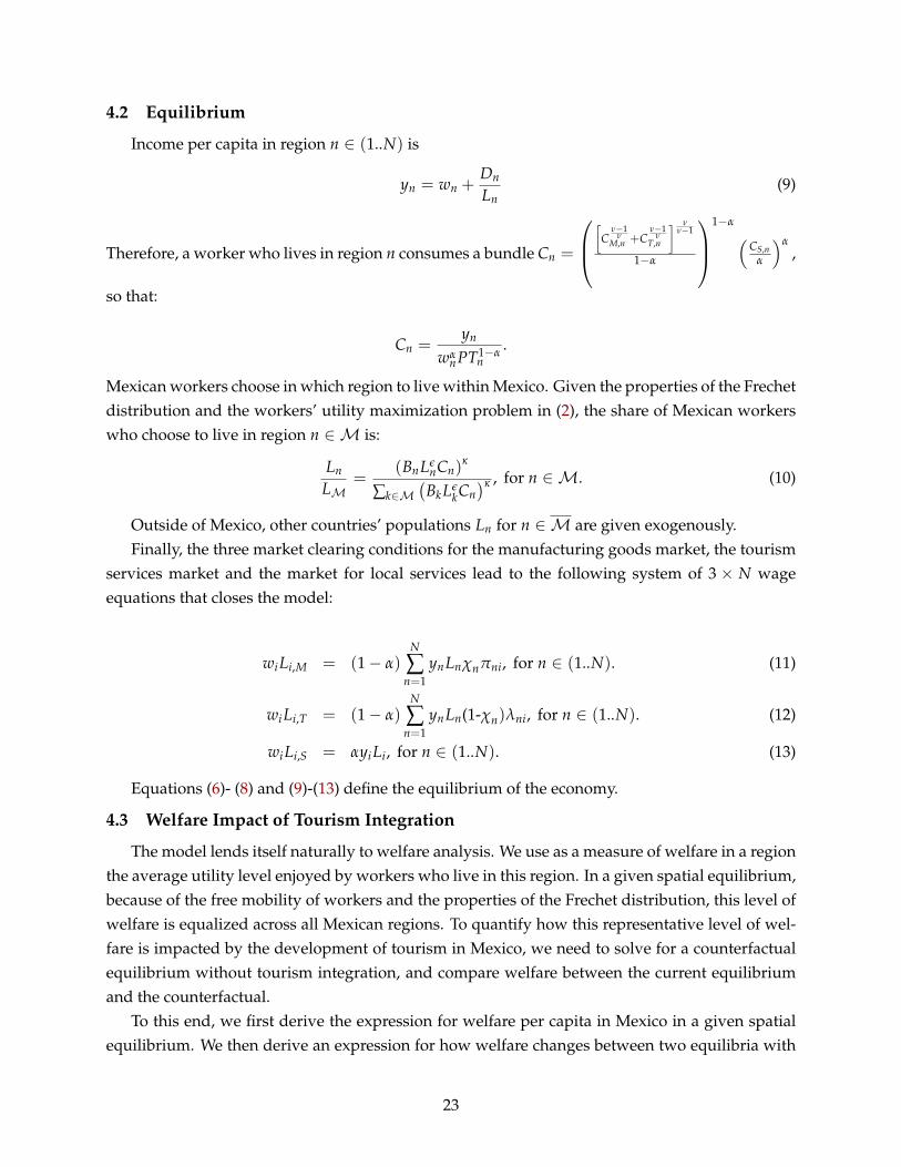
4.2 Equilibrium

Income per capita in region n ∈ (1..N) is

yn = wn +Dn

Ln(9)

Therefore, a worker who lives in region n consumes a bundle Cn =

[

Cν−1

νM,n +C

ν−1ν

T,n

] νν−1

1−α

1−α (

CS,nα

)α,

so that:

Cn =yn

wαnPT1−α

n.

Mexican workers choose in which region to live within Mexico. Given the properties of the Frechetdistribution and the workers’ utility maximization problem in (2), the share of Mexican workerswho choose to live in region n ∈ M is:

Ln

LM=

(BnLεnCn)

κ

∑k∈M(

BkLεkCn)κ , for n ∈ M. (10)

Outside of Mexico, other countries’ populations Ln for n ∈ M are given exogenously.Finally, the three market clearing conditions for the manufacturing goods market, the tourism

services market and the market for local services lead to the following system of 3 × N wageequations that closes the model:

wiLi,M = (1− α)N

∑n=1

ynLnχnπni, for n ∈ (1..N). (11)

wiLi,T = (1− α)N

∑n=1

ynLn(1-χn)λni, for n ∈ (1..N). (12)

wiLi,S = αyiLi, for n ∈ (1..N). (13)

Equations (6)- (8) and (9)-(13) define the equilibrium of the economy.

4.3 Welfare Impact of Tourism Integration

The model lends itself naturally to welfare analysis. We use as a measure of welfare in a regionthe average utility level enjoyed by workers who live in this region. In a given spatial equilibrium,because of the free mobility of workers and the properties of the Frechet distribution, this level ofwelfare is equalized across all Mexican regions. To quantify how this representative level of wel-fare is impacted by the development of tourism in Mexico, we need to solve for a counterfactualequilibrium without tourism integration, and compare welfare between the current equilibriumand the counterfactual.

To this end, we first derive the expression for welfare per capita in Mexico in a given spatialequilibrium. We then derive an expression for how welfare changes between two equilibria with

23

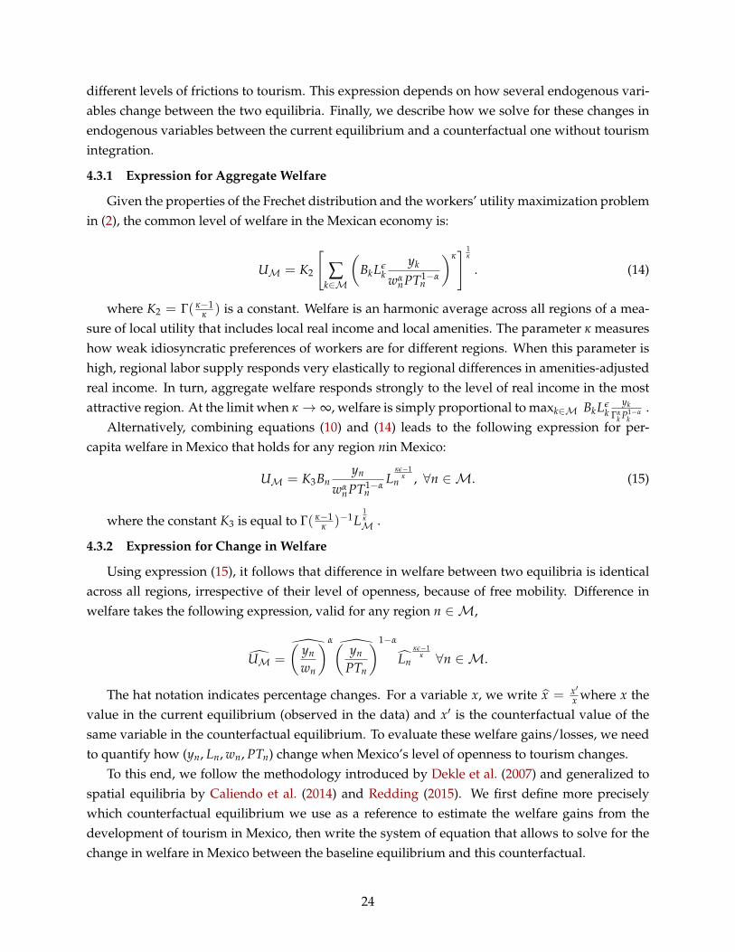
different levels of frictions to tourism. This expression depends on how several endogenous vari-ables change between the two equilibria. Finally, we describe how we solve for these changes inendogenous variables between the current equilibrium and a counterfactual one without tourismintegration.

4.3.1 Expression for Aggregate Welfare

Given the properties of the Frechet distribution and the workers’ utility maximization problemin (2), the common level of welfare in the Mexican economy is:

UM = K2

[∑

k∈M

(BkLε

kyk

wαnPT1−α

n

)κ] 1

κ

. (14)

where K2 = Γ( κ−1κ ) is a constant. Welfare is an harmonic average across all regions of a mea-

sure of local utility that includes local real income and local amenities. The parameter κ measureshow weak idiosyncratic preferences of workers are for different regions. When this parameter ishigh, regional labor supply responds very elastically to regional differences in amenities-adjustedreal income. In turn, aggregate welfare responds strongly to the level of real income in the mostattractive region. At the limit when κ → ∞, welfare is simply proportional to maxk∈M BkLε

kyk

Γαk P1−α

k.

Alternatively, combining equations (10) and (14) leads to the following expression for per-capita welfare in Mexico that holds for any region nin Mexico:

UM = K3Bnyn

wαnPT1−α

nL

κε−1κ

n , ∀n ∈ M. (15)

where the constant K3 is equal to Γ( κ−1κ )−1L

1κM .

4.3.2 Expression for Change in Welfare

Using expression (15), it follows that difference in welfare between two equilibria is identicalacross all regions, irrespective of their level of openness, because of free mobility. Difference inwelfare takes the following expression, valid for any region n ∈ M,

UM =

(yn

wn

)α(yn

PTn

)1−α

Lnκε−1

κ ∀n ∈ M.

The hat notation indicates percentage changes. For a variable x, we write x = x′x where x the

value in the current equilibrium (observed in the data) and x′ is the counterfactual value of thesame variable in the counterfactual equilibrium. To evaluate these welfare gains/losses, we needto quantify how (yn, Ln, wn, PTn) change when Mexico’s level of openness to tourism changes.

To this end, we follow the methodology introduced by Dekle et al. (2007) and generalized tospatial equilibria by Caliendo et al. (2014) and Redding (2015). We first define more preciselywhich counterfactual equilibrium we use as a reference to estimate the welfare gains from thedevelopment of tourism in Mexico, then write the system of equation that allows to solve for thechange in welfare in Mexico between the baseline equilibrium and this counterfactual.

24

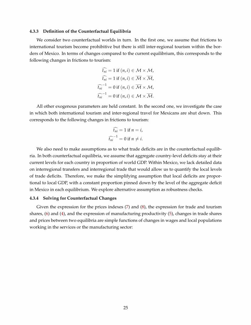
4.3.3 Definition of the Counterfactual Equilibria

We consider two counterfactual worlds in turn. In the first one, we assume that frictions tointernational tourism become prohibitive but there is still inter-regional tourism within the bor-ders of Mexico. In terms of changes compared to the current equilibrium, this corresponds to thefollowing changes in frictions to tourism:

tni = 1 if (n, i) ∈ M×M,

tni = 1 if (n, i) ∈ M×M,

tni−1

= 0 if (n, i) ∈ M×M,

tni−1

= 0 if (n, i) ∈ M×M.

All other exogenous parameters are held constant. In the second one, we investigate the casein which both international tourism and inter-regional travel for Mexicans are shut down. Thiscorresponds to the following changes in frictions to tourism:

tni = 1 if n = i,

tni−1

= 0 if n 6= i.

We also need to make assumptions as to what trade deficits are in the counterfactual equilib-ria. In both counterfactual equilibria, we assume that aggregate country-level deficits stay at theircurrent levels for each country in proportion of world GDP. Within Mexico, we lack detailed dataon interregional transfers and interregional trade that would allow us to quantify the local levelsof trade deficits. Therefore, we make the simplifying assumption that local deficits are propor-tional to local GDP, with a constant proportion pinned down by the level of the aggregate deficitin Mexico in each equilibrium. We explore alternative assumption as robustness checks.

4.3.4 Solving for Counterfactual Changes

Given the expression for the prices indexes (7) and (8), the expression for trade and tourismshares, (6) and (4), and the expression of manufacturing productivity (5), changes in trade sharesand prices between two equilibria are simple functions of changes in wages and local populationsworking in the services or the manufacturing sector:

25

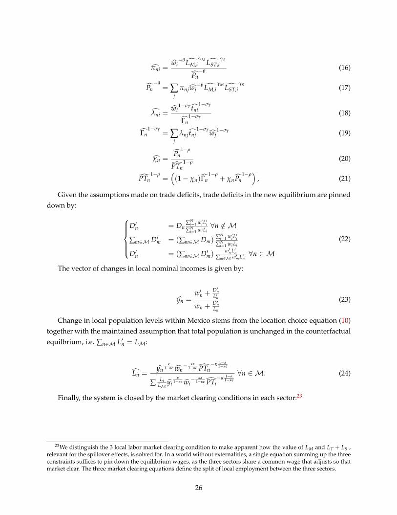
πni =wi−θ LM,i

γM LST,iγS

Pn−θ

(16)

Pn−θ

= ∑j

πnjwj−θ LM,i

γM LST,iγS (17)

λni =wi

1−σT tni1−σT

Γn1−σT

(18)

Γn1−σT

= ∑j

λnj tnj1−σT wj

1−σT (19)

χn =Pn

1−ρ

PTn1−ρ

(20)

PTn1−ρ

=((1− χn)Γn

1−ρ+ χnPn

1−ρ)

, (21)

Given the assumptions made on trade deficits, trade deficits in the new equilibrium are pinneddown by:

D′n = Dn∑N

i=1 w′i L′i

∑Ni=1 wi Li

∀n /∈ M

∑m∈M D′m = (∑m∈M Dm)∑N

i=1 w′i L′i

∑Ni=1 wi Li

D′n = (∑m∈M D′m)w′n L′n

∑m∈M w′m L′m∀n ∈ M

(22)

The vector of changes in local nominal incomes is given by:

yn =w′n +

D′nL′n

wn +D′nLn

(23)

Change in local population levels within Mexico stems from the location choice equation (10)together with the maintained assumption that total population is unchanged in the counterfactualequilbrium, i.e. ∑n∈M L′n = LM:

Ln =yn

κ1−κε wn

− κα1−κε PTn

−κ 1−α1−κε

∑ LiLM

yiκ

1−κε wi− κα

1−κε PTi−κ 1−α

1−κε

∀n ∈ M. (24)

Finally, the system is closed by the market clearing conditions in each sector:23

23We distinguish the 3 local labor market clearing condition to make apparent how the value of LM and LT + LS ,relevant for the spillover effects, is solved for. In a world without externalities, a single equation summing up the threeconstraints suffices to pin down the equilibrium wages, as the three sectors share a common wage that adjusts so thatmarket clear. The three market clearing equations define the split of local employment between the three sectors.

26

w′i L′T,i = (1− α)

N

∑n=1

(w′nL′n + D′n)(1− χ′n)λ′ni. (25)

w′i L′M,i = (1− α)

N

∑n=1

(w′nL′n + D′n)χ′nπ′ni. (26)

w′i L′i,S = α(w′i L

′i + D′i) (27)

L′i = L′M,i + L′T,i + L′S,i (28)

Knowing the values of (πnj, λnj, χn, wn, LM,n, LT,n, LS,n, Dn) in the baseline equilibrium, the pa-rameters of the model (α, σ, θ, ν, κ

1−κε ) and the change in frictions tni, the system of equations(16)-(26) defines the counterfactual equilibrium. This equilibrium is unique under a set of param-eter restrictions, as shown in the Appendix.

4.4 Distribution of the Gains from Tourism across Groups

We extend the framework to model various subgroups of the population, following Galle et al.(2014).

[Work in progress.]

5 Estimation and Calibration of the Model

5.1 Methodology

To quantify the long run economic impact of tourism in Mexico, the analysis proceeds in threeconsecutive steps. In the first step, we calibrate the model to the reference equilibrium corre-sponding to the current level of trade and tourism frictions, using wages, employment and tradedata on the one hand, and estimates for the trade elasticity θ and the tourism elasticity σT on theother hand. We detail below how we use the data at hand to calibrate the model. Importantly,this step does not require estimating the spatial labor supply elasticity nor the spillover function.This first step allows us to recover a vector of –possibly endogenous– model-based manufacturingproductivities Mn and a set of local demand shifters for tourism An.

In the second step, we estimate the reduced form spatial labor supply elasticity κ1−κε . We

derive an estimating equation from the model, and exploit the instrumental variables for localbeach quality that we discuss in Section 3 as a set of exogenous shifters to local real wages toidentify κ

1−κε . This procedure requires an estimate of the local price indices for tourism and otherconsumption for which sufficiently rich available data do not exist in our empirical setting.24 Tocircumvent this issue, we use the model-consistent price indices that we calibrated in the first step.Importantly, this step does not require knowledge of the spillover function.

In the third step, armed with all of the relevant parameters of the model, we investigate the ex-istence of productivity spillovers both within manufacturing and between tourism and manufac-turing using indirect inference. We use two sets of reduced form empirical estimates from section

24Note that consumption microdata such as the AC Nielsen Mexican consumer panel focus on relatively large citiesand would only cover a fraction of coastal municipalities (less than 20).

27

3 to calibrate the spillover function. The first empirical fact is the estimated elasticity of manufac-turing GDP with respect to tourism GDP in the current spatial equilibrium (Table 8). The secondempirical fact is the orthogonality of the distribution of economic activity pre-tourism to currenttourism GDP when instrumented by a set of exogenous shifters of tourism revenues (Table 5). Wereplicate the first empirical fact using the calibrated model at the current level of frictions, andthe second empirical fact using the model with the same parameters, but simulated at a counter-factual equilibrium corresponding to prohibitive inter-regional tourism frictions. Matching thesereduced form moments imposes a strong discipline on how manufacturing productivities Tn canbe decomposed between an exogenous part, independent of the level of economic activity, and anendogenous part, coming from within and cross-sector production externalities.

5.2 Calibration of the Baseline Equilibrium

To calibrate the baseline equilibrium, we follow a methodology close to the one laid out by(Redding, 2015). Using direct data on (wn, LM,n, LT,n, LS,n, Dn), a parametric specification for thetrade and tourism frictions (τij, tij) and estimates for the elasticities (θ, σT, ρ), we recover the onlyvectors of local manufacturing productivities and local demand shifters for tourism (Mn, An), forn ∈ M, that are consistent with the data (up to a normalization factor).

5.2.1 Data

The model is calibrated to the mean outcomes for 2000 and 2010 as the baseline period.25 Inorder to limit the computing requirements, we aggregate the data coming from each of the 2455Mexican municipalities described in the reduced form empirical exercise into a set of 300 regions.In particular, we keep the 150 coastal municipalities unchanged, but aggregate the interior mu-nicipalities to 150 economic centers that are located at the centroids of the largest 150 interiormunicipalities (in terms of mean GDP in 2000 and 2010).26 As we show in the Online Appendix,this is without loss of generality as the key empirical moments that we match with the model areidentified off variation among coastal municipalities.

Mincerized wages are our preferred measure of local wages. They allow to control for sourcesof heterogeneity that the model does not account for. Employment is our preferred measure of lo-cal population for all Mexican municipalities. To estimate the share of employment in tourism andmanufacturing in each Mexican region, we follow the assumption already made above, that hotelsales are a constant proportion of local tourism GDP. We then proxy for the share of employmentin tourism (resp. manufacturing) in each Mexican region by computing the ratio of hotel sales tomanufacturing GDP in each region, and scaling these ratios so that in the aggregate, the ratio oftourism GDP to manufacturing GDP equals the one from the data. Finally, we calibrate the shareof employment in local services such that aggregate GDP in all services matches the aggregatedata for Mexico.

For simplicity, we aggregate all countries but Mexico into a “Rest of the World” (“RoW”) aggre-gate. Population of RoW is adjusted so that the ratio of GDP of Mexico to the GDP of RoW equals

25The detailed procedure and data sources are reported in the Online Appendix.26The remaining interior regions are assigned to the closest of the 150 interior centroids.

28

the ratio computed in the data. The shares of workers in the manufacturing and tourism industryfor RoW are calibrated to the share of GDP in each industry. Finally, the share of consumption oflocal services is read from the share of world GDP in services, tourism excluded.

There is no available data on bilateral trade between municipality pairs within Mexico. Tocalibrate these shares using the available data, we use a parametric specification of the frictions totrade and tourism within Mexico. There is a long literature finding robust evidence that tradeflows decay with distance with a constant elasticity close to 1 ((Mayer, 2014)). We thereforeparametrize trade fictions within Mexico such that

τ−θnj = d−DM

nj , for (n, j) ∈ M×M,

where DM = 1, where dnj is the distance between the centroid of the two municipalities n and j.We follow a similar parametrization for tourism flows. To estimate the distance decay of tourismflows, we run a model-based gravity equation on country-level bilateral tourism exports, takingthe log of equation (4) aggregated at the country level:

logEH,knt = δkt + ζnt − DH ln dnk + Xnk + νknt, (29)

where EH,knt is the spending of country k on tourism in country n in year t, δkt is an country oforigin-by-year fixed effect, ζnt is a destination country-by-year fixed effect, Xnk are three dummyvariables capturing other sources of frictions to international tourism besides distance, such aswhether countries share a common border, language or colonial ties. Finally, dnk is our regressorof interest, the distance between country n and k. As can be seen in Figure 2, tourism flows arevery clearly subject to gravity, with a tightly estimated distance decay elasticity of DH = 1.46. Wetherefore parametrize tourism fictions within Mexico as varying with distance, such that:

t1−σnj = d−DH

nj , for (n, j) ∈ M×M.

Finally, international frictions, in tourism and in manufacturing, are calibrated so that the modelexactly matches the aggregate trade data in manufactured goods and tourism between Mexicoand the rest of the world.27 The aggregate Mexican deficit is also directly taken from the data.28

5.2.2 Tourism and Trade Elasticities

We use the panel data on country-level bilateral tourism exports to estimate the tourism elas-ticity. Equation (4) leads to the following estimating equation for σT:

logEH,knt = δkt + ζnk + (1− σT) ln wnt + νknt, (30)

27Given that we aggregate all international trade flows into a single foreign country, we further make the assump-tion that frictions to international trade between Mexico and that synthetic country are symmetric and do not varysystematically across Mexican regions.

28As mentioned above, given data availability, we assume that local trade deficits within Mexico are in constantproportion of local GDP. This pins down the full vector of Dn.

29

where EH,kn is the spending of country k on tourism in country n during time t, δkt is an origin-by-time fixed effect (e.g. capturing productivity shocks), ζnk is an origin-by-destination fixed effect(e.g. capturing distances or cultural proximity), ln wnt is the relative consumption price of tourismservices across destinations and νknt is a mean zero measurement error term. To empirically mea-sure ln wnt, we use country-level PPP rates for final consumption goods that the InternationalPrice Comparison (ICP) program computes for all 115 countries over the period 1990-2011 in ourdatabase. The ICP constructs this measure, PPPnt as the number of units of a country n’s currencyrequired to buy the same basket of goods and services in the domestic market as one US Dollarwould buy in the United States. To measure ln wnt, we take the log of (1/PPPnt). Given the inclu-sion of origin-by-period and origin-by-destination fixed effects, this measure effectively captures(with some error) relative consumption price changes across different destination countries fromthe point of view of a given origin-by-time cell.

The main concern for the identification of (1− σT) is that changes in consumption prices acrossdestinations are correlated with other factors that may increase or decrease bilateral tourism flowsin the error term. For example, if prices in a destination increase at the same time that travelers atthe origin become more likely to travel to the destination for other reasons (e.g. due to businesstravel or attractiveness), this would lead to an upward biased estimate of (1− σT) (towards zero).

The first thing we do to address this concern is to include a basic control for time changing eco-nomic conditions in the destination countries, by including the log of country GDP as a control.Second, to address remaining concerns, in addition to the very likely concern of measurement er-ror in our measure of ln wnt, we use nominal exchange rate changes across destination countrieswith respect to the US Dollar, ln ent, as an instrumental variable for ln (1/PPPnt). The exchangerates are used as part of the PPP rate construction by the ICP, so that we can expect a strong firststage. The exclusion restriction is that differential exchange rate changes across different destina-tion markets to not affect bilateral tourism expenditure except through relative price changes oftourism services. To further assess the validity of this assumption, we also estimate specification(30) after restricting attention to what we label touristic destinations: i.e. destinations for whichmore than 80 percent of total travel inflows are due to leisure rather than business travel. Finally,to allow for tourist flows to respond to relative price information across destination markets withsome time lag, we also estimate specifications in which we lag the independent variable by 1-5years.

Table 11 presents the estimation results. We find a moderately negative tourism elasticity thatreaches σT = 1.7 when we lag the relative destination price changes by 3-4 year (1.5 with lesserlags). These results are confirmed with a slightly lower point estimate of 1.6 once we restrict at-tention to destinations with more than 80 of travel inflows driven by leisure rather than businesspurposes (even though we start to get problems with sparseness here). The preliminary conclu-sion we draw from these first estimations is that the tourism elasticity appears to be significantlylower than common estimates of the trade elasticity for flows in goods.

The upper-nest elasticity that governs the substitution patterns between manufacturing andtourism has to be smaller than the lower nest elasticity of σT = 1.7. We choose a value of ρ = 1.5

30

in our main specification. As for the trade elasticity for flows of goods, we use an existing estimatefrom the literature of θ = 6.1 (Shapiro, 2014; Adao et al., 2015). As a robustness check, we alsorevisit our quantifications using a range of alternative parameter combinations of (σT, ρ, θ).

Armed with the calibrated values for (wn, LM,n, LT,n, LS,n, Dn, τnm, tnm) and estimates for theelasticities (θ, σT, ρ) presented above, we use numerical methods to recover the only (up to anormalization factor) vectors of local manufacturing productivities and local demand shifters fortourism (Mn, An), for n ∈ M, that are consistent with the data.

5.2.3 Spatial Labor Supply Elasticity

In the second step of the analysis, we estimate the spatial labor supply elasticity. This elasticitywas not needed to back out manufacturing productivities and local demand shifters for tourism(Tn, An), but is necessary to compute counterfactual equilibria and their welfare consequences.The estimating equation for the spatial labor supply elasticity is derived from Equation (10) of themodel. It leads to the following estimating equation:

log Ln = Ko +1

1− κεlog Bn +

κ

1− κεlog

(wn

Pn

)+ νn for n∈ M (31)

where Pn is the local price index in region n and νn is a mean zero measurement error term. TheMincerized wages are observed in our data. Price indexes are not, but they are pinned down inthe calibrated model. We use these to infer the vector of local real incomes, wn

Pn.

Note that the “raw” spatial labor supply elasticity κ is not identified separately from the amen-tiy externality ε. For our purposes, and in particular for welfare computations, we do not need aseparate estimate of these two elasticities, but only an estimate of κ

1−κε . The main concern tocausally identify κ

1−κε in specification (31) is that our measure of real wages is correlated with un-observed local amenities Bn. All else equal, this would lead to a downward bias (towards zero)in our estimate of the spatial labour supply elasticity. The second major concern is measurementerror in our construction of local real wages across municipalities in 2000 and 2010. Both the Min-cerized nominal wage measure and especially our construction of the local price indices usingtraded good and tourism market access measures are likely to be subject to measurement error.

To address these concerns, we exploit the identifying assumption that our measures of localbeach quality only affect local employment through either their affect on nominal wages, or theiraffect on the local price index (both for tourism services and for traded goods). Notice that thisempirical strategy also allows for tourism to affect local amenities, but only through its effect onlocal real wages and the resulting changes in local populations. This is captured as part of ourreduced form labor supply elasticity, κ

1−κε , where ε captures the change in local amenities due tochanges in the local population density.

Table 12 presents the estimation results. We estimate large and significant positive point es-timates for the expression κ

1−κε . The point estimates for κ1−κε is an order of magnitude larger in

the IV specifications relative to the OLS specification. This is consistent with both downwardbias due to unobserved local amenities as well as significant measurement error in our real wagemeasures. The IV point estimates suggest that the spatial labour supply elasticity across Mexican

31

municipalities, κ1−κε , is about 10.2 for employment.

Finally, we further assess the potentially remaining concern that tourism may affect localamenities in Bn through direct channels that are not captured by its effect on the local popula-tion (through ε). For example, tourism could have either positive or negative direct effects onlocal amenities through its affect on the density of local restaurants and stores (positive), envi-ronmental degradation (negative) or congestion that is more intense per capita than in absence oftourism (negative). To further investigate these concerns, we are collecting data from several ad-ministrative sources aimed at capturing differences in positive or negative local amenities (workin progress).

5.2.4 Agglomeration Economies

Manufacturing is potentially subject to within and cross-sector production externalities. Thedevelopment of tourism may have indirect effects on manufacturing production by affecting thescale of local production across different sectors. We have modelled that possibility in a reduced-form way by assuming that productivity in manufacturing may depend on the scale of local eco-nomic activity in manufacturing and services, through the productivity function:

Mn = MonLγM

M,nLγSST,n.

Through the calibration of the baseline equilibrium, we recover a vector of local manufactur-ing productivities.29 To fully characterize the effect of tourism on long-run economic outcomes,we need to estimate the within and cross-sector spillovers on manufacturing (γM, γS).

To do so, we propose a strategy based on indirect inference. We note that current-day popula-tions are strongly correlated with the set of beach IVs that we have used in Section 3. At the sametime, Table 5 establishes that these correlations were insignificant or marginally negative beforethe development of tourism in Mexico. This suggests a way to back out the productivity parame-ters using indirect inference. We develop a procedure that aims to match the results of the placeboregressions using a model-based counterfactual equilibrium where tourism frictions are assumedto be prohibitive.

We denote βa as the coefficients of the regressions reported in Table 5, where a ranges from 1to 6 and indexes the set of beach IVs used in our empirical strategy (where 1 is the island IV and2-5 are the four beach IVs). Recall that the system of equations (16)-(26) allows us to compute nu-merically the distribution of wages and population in Mexico in a counterfactual equilibrium withprohibitive tourism frictions, assuming all other exogenous parameters remain unchanged. Thisprocedure can be implemented for different combinations of the externality parameters (γM, γS).We write the resulting counterfactual vector of populations in Mexico as a function of the intensityof spillovers, of the level tourism frictions in the counterfactual equilibrium (tc

ij ), and of all otherparameters of the model summarized by ξc. We assume that these parameters are exogenous andstay unchanged in the counterfactual equilibria we study, i.e. that ξc = ξo. The counterfactual

29The vector of productivities is pinned down up to a multiplicative constant.

32

population then becomes the function:

Lcn = Lc

n(γM, γS, tcij, ξc).

Having recovered this function of parameters (γM, γS), we use indirect inference to look for esti-mates ( ˆγM, γS) such that:

E[

Lcn( ˆγM, γS, tc

ij, ξc).za

]= βa, for a=1..6,

where za is the ath instrumental variable that we use in the reduced form analysis, and βa arethe values we target in the procedure. They are related to the results of the placebo regressionspresented in Table 5. We examine two specifications. In the first, we use βa = 0 as the likely moreconservative approach to estimate the extent of tourism spillovers. In the second specification, weuse the actual point estimates of the regressions (which tend to be negative) as a target, i.e. βa = βa

. In both cases, to find the best fitting parameters ( ˆγM, γS) , we have to solve for a counterfactualequilibrium for each possible parameter combination. We then run the following regressions onthe counterfactual population data, where outcomes in a counterfactual equilibrium are denotedwith a superscript c:

log Lcn = α + βc

alog za + εca.

For each set of parameters ( ˆγM, γS), this yields an estimate of the regression coefficient βCa . We

finally minimize the distance between βCa and βa , by minimizing the loss function:

L( ˆγM, γS, tcij, ξc) = ∑

a

(βc

a( ˆγM, γS, tcij, ξc)− βa

seca

)2

,

where secais the standard error of the estimate βc

a. This scaling ensures that the procedure weightseach regression coefficient appropriately. Intuitively, imprecise estimates are weighted less in theminimization routine. Results of this procedure are reported graphically in Figure 3.30 The bestfitting combination of parameters over this grid to match the zero point estimates is γM = .05 andγS = .16. When the target is to match the actual point estimates of the regression, the best fittingcombination of parameters is γM = .075 and γS = .2.

These results present evidence of sizable within and cross-sector spillover effects in Mexicanmanufacturing that rationalize the observed effects of tourism on regional manufacturing activityin Mexico. These findings underlie the strong observed effects of tourism development in Mexicoon the reallocation of economic activity across space. The important remaining question is on theaggregate effect of these spillovers, to which we now turn in the aggregate welfare analysis.

30To minimize computing power requirements, we look for the parameter combination that delivers the best fitover a grid of possible values for γM and γS ranging from 0 to .25.

33

6 QuantificationThis section proceeds to the quantification of the long-run economic consequences of tourism

in Mexico. We first present our baseline results for the welfare gains from tourism, and decomposethis effect into the underlying channels. We then report a number of additional quantification re-sults to document the sensitivity across alternative parameter combinations. Finally, we analyzethe distribution of the gains from tourism across different groups of the Mexican society.

6.1 Gains from Tourism

To evaluate the welfare gains brought about by the development of tourism in Mexico, wecompare the level of welfare in a series of counterfactual equilibria to the one in the baselinecurrent-day equilibrium. The counterfactual equilibria we consider are ones in which the extentof the development of tourism is limited compared to today’s equilibrium. We examine two cases.In the first one, Mexico is closed to international tourism but within-country tourism is still pos-sible. In the second one, tourism frictions are prohibitive both nationally and internationally. Foreach case, we conduct the analysis under the assumption that either γM = .05 and γS = .16, orthat γM = .075 and γS = .2. The difference in aggregate welfare between a counterfactual equil-brium and the baseline equlibrium represents the welfare loss from going back to a world withouttourism (resp. without international tourism). For the clarity of exposure, we refer to the inverseof these numbers as the ‘gains from tourism’.

Table 13 presents the quantification of the gains from tourism. In the first column, we re-port the gains from tourism integration both domestically and internationally. In column 2, welimit the analysis to international tourism. The gains from the development of tourism amountto about 2.9% welfare gains per capita. The development of international tourism contributes tohalf of these gains, or 1.5%, in our preferred specification. Table 13 also decomposes these welfareresults into the classical welfare gains, and those that come from spillover effects. Interestingly,while the spillovers lead to large regional reallocations of production in Mexico, their aggregateeffect on Mexican welfare is largely muted. In the absence of spillovers, the welfare gains fromtourism development would have amounted to 2.4%. This is reminiscent of the finding in (Kline& Moretti, 2014) that strong local agglomeration effects may be offset in the aggregate.

Note, however, that the result is not functional form driven but dictated by the data. To illus-trate this point, we show below what would have happened with strong cross-sector spillovers ofγS = .15 but no within-sector productivity externality in manufacturing (γM = 0). Conversely,we also study the case where within-sector externalities are high (γM = 0.15) but cross-sectoralspillovers are absent (γS = 0). Finally, we report the case without spillovers where the classicalmarket integration effect is the only source of the gains from tourism.

Table 14 illustrates the impact that tourism would have had on regional outcomes for thesedifferent values of spillovers. Specifically, it reports the estimates of the following regressions:

∆logGDPn = βA0 + βA

1 logGDPTourismn + Xn + εn,

and

34

∆logGDPManun = βM0 + βM

1 logGDPTourismn + Xn + εn,

where the local GDP for tourism is instrumented with the beach IV. We run these regressions fora range of parameter values for the cross and within-sector spillovers. In addition to the pointestimates, Table 14 also reports what would have been the welfare gains from tourism integrationin each case. Panel A corresponds to the outcomes of the first regression, on total local GDP, andPanel B corresponds to Manufacturing GDP only.

A first scenario that we explore is the one without any form of spillovers. In that case, tourismleads to the growth of local GDP (first column of Panel A), but this is only driven by the tourismsector. The effect of tourism on local manufacturing growth is negative (first column of Panel B),which would go against the reduced form empirical evidence presented in Section 3. This negativeimpact is driven by the classic Dutch disease mechanism: as local demand for tourism increases,it drives up wages which adversely affects local traded goods production. In turn, manufacturinglocates in regions in which there is no upward pressure on wages coming from the developmentof tourism.

Another focal case is the situation in which we shut down any spillover going from tourismto manufacturing (γS = 0), but allow for agglomeration economies within manufacturing (’local-ization externalities’) (γM > 0). The corresponding results are reported in the second column ofboth Panels. The development of tourism barely leads to an increase in local GDP (second col-umn of Panel A), as it leads to a strong negative effect on local manufacturing growth (secondcolumn of Panel B). The underlying reason is that the Dutch disease effect described above is re-inforced here by the presence of agglomeration externalities in manufacturing. Manufaturing andtourism do not coagglomerate. In terms of aggregate welfare, the existence of within-sector ag-glomeration economies in manufacturing in this case leads to a negative aggregate impact of thedevelopment of tourism: the welfare gains from tourism are reduced from 2.4% to 1% compared towhat the classical gains from integration would have been in the absence of production external-ities. This illustrates the case when tourism acts as a special case of the Dutch disease. Resourcesare reallocated away from traded goods production to tourism. Due to localization economieswithin manufacturing, this has negative implications for productivity in traded goods production- because agglomeration economies are present in manufacturing but absent in tourism-relatedservices production.

The third column reports the polar opposite case where only cross-sector spillovers are at play.In that case, manufacturing GDP grows more in places in which tourism develops (third columnof Panel B). This positive impact of the development of tourism on local manufacturing growthcomes from a productivity effect: manufacturing becomes more productive where tourism de-velops. In turn, in the aggregate, this leads to additional welfare benefits of the developementof tourism, as it leads to a growth in manufacturing productivity that would not have otherwiseoccurred. Quantitatively, the welfare gains from tourism are in that case about 1.5 times higherthan the classical gains from market integration without spillover effects.

35

These results are informative about the underlying channels of the gains from tourism that weestimate for the Mexican case (γM = .075 and γS = .2). Spillovers from tourism to manufacturingare strong enough to generate co-agglomeration patterns between touristic regions and manu-facturing centers, as attested by the positive impact of tourism on local manufacturing growth.On the other hand, manufacturing is also estimated to be subject to within-sector agglomera-tion economies. While this effect tends to reinforce the observed coagglomeration pattern due totourism, it also implies that the aggregate welfare effect of tourism on manufacturing productivityis muted. As we have seen above, the presence of positive own-sector spillovers pushes towardreducing the gains from tourism integration, whereas the presence of cross-industry spillovershas the opposite effect. They both work through the reallocation of workers from one sector to theother at the aggregate level across all Mexican regions. Here, both effects are at play and tend tooffset one another in the aggregate. While these two agglomeration forces reinforce one anotherfor the local effects of tourism on traded goods production and total GDP, the aggregate gainsfrom tourism in Mexico are therefore largely comparable to what would have prevailed withoutspillovers (reported in columnn 1 of Table 14).

6.2 Robustness across Alternative Parameters

[Work in progress.]

6.3 Distribution of the Gains from Tourism

[Work in progress.]

7 ConclusionMuch of the existing social sciences literature on tourism and economic development has been

critical about tourism’s long run implications, especially in developing countries. At the sametime, governments around the world, and to a lesser extent international aid organizations, areshowing widespread interest in tourism and have committed substantial amounts of public fundsfor national and regional tourism promotion. Somewhat surprisingly in this context, both theexisting literature and tourism policies are currently based on limited empirical evidence.

This paper combines a spatial equilibrium model of trade in goods and tourism services witha rich collection of Mexican microdata and a new empirical strategy in order to contribute to ourunderstanding of the long term economic consequences of tourism in a developing country. Toestimate the reduced form effects of differences in long term tourism exposure in today’s cross-section of Mexican municipalities, we exploit oceanographic and geological variation in beachquality along the Mexican coastline and use high-resolution historical satellite data to constructa number of instrumental variables. To guide the estimation of tourism’s welfare implications,we then write down a spatial equilibrium model, inform its calibration using the reduced formmoments and explore general equilibrium counterfactuals.

The analysis gives rise to several new findings. We find that tourism causes large and signifi-cant increases in long run real economic activity across regions. Contrary to much of the existing

36

literature, these local effects are driven by sizable multiplier effects on traded goods production.Through the lens of the model, these multiplier effects provide evidence of positive spillover ef-fects of tourism on manufacturing production. In particular, we estimate significant cross-sectorspillovers in addition to within-sector localization economies within manufacturing. Interestingly,while these two sources of agglomeration economies reinforce one another leading to large ob-served reallocations of manufacturing and total GDP towards tourism centers, we find that theylargely offset one another for the aggregate implications of tourism. That is, while tourism leadsto sizable gains in agglomeration economies at the local level, these gains are largely offset byreductions in agglomeration economies at the national level, so that the aggregate welfare gainsfrom tourism are mainly driven by a classical market integration effect. Finally, we find that thesegains from tourism are unevenly distributed across groups of gender, education and ethnicity inthe Mexican society. Overall, we find that the gains from tourism are on average positive for allgroups, but significantly regressive when taking into account the existing distribution of nominalincomes across these groups.

The analysis serves to inform currently ongoing policy debates in two central ways. First, weprovide credible empirical evidence on the long term effects of tourism activity on economic out-comes both across Mexican regions and at the aggregate national level. Second, the methodologythat we propose in this paper provides a useful empirical tool with wide applicability to study anumber of open questions on the regional and aggregate effects of tourism or similar shocks inother empirical settings and for additional economic outcomes of interest.

ReferencesAdao, R., Costinot, A., & Donaldson, D. (2015). Nonparametric counterfactual predictions in neoclas-

sical models of international trade (Tech. Rep.). National Bureau of Economic Research.

Allcott, H., & Keniston, D. (2014). Dutch disease or agglomeration? the local economic effects of naturalresource booms in modern america (Tech. Rep.). National Bureau of Economic Research.

Allen, T., & Arkolakis, C. (2014). Trade and the topography of the spatial economy. The QuarterlyJournal of Economics, 1085, 1139.

Anderson, S. P., De Palma, A., & Thisse, J. F. (1992). Discrete choice theory of product differentiation.MIT press.

Arezki, R., Cherif, R., & Piotrowski, J. (2009). Tourism specialization and economic development:Evidence from the unesco world heritage list (No. 9-176). International Monetary Fund.

Atkin, D., Faber, B., & Gonzalez-Navarro, M. (2015). Retail globalization and household welfare:Evidence from mexico. UC Berkeley mimeo.

Caliendo, L., Dvorkin, M., & Parro, F. (2015). The impact of trade on labor market dynamics (Tech.Rep.).

Caliendo, L., & Parro, F. (2014). Estimates of the trade and welfare effects of nafta. The Review ofEconomic Studies, rdu035.

Caliendo, L., Parro, F., Rossi-Hansberg, E., & Sarte, P.-D. (2014). The impact of regional and sectoralproductivity changes on the us economy (Tech. Rep.). National Bureau of Economic Research.

37

Caselli, F., & Michaels, G. (2009). Do oil windfalls improve living standards? evidence from brazil (Tech.Rep.). National Bureau of Economic Research.

Copeland, B. R. (1991). Tourism, welfare and de-industrialization in a small open economy. Eco-nomica, 515–529.

Davis, M. A., & Ortalo-Magné, F. (2011). Household expenditures, wages, rents. Review of EconomicDynamics, 14(2), 248–261.

Dekle, R., Eaton, J., & Kortum, S. (2007). Unbalanced trade. American Economic Review, 97(2),351–355.

DFID. (1999). Tourism and poverty alleviation: Untapped potential. DFID, London.

Dieke, P. (2000). The political economy of tourism development in africa. Cognizant CommunicationCorporation.

Donaldson, D. (in press). Railroads of the raj: Estimating the impact of transportation infrastruc-ture. American Economic Review.

Eaton, J., & Kortum, S. (2002). Technology, geography, and trade. Econometrica, 1741–1779.

Eilat, Y., & Einav, L. (2004). Determinants of international tourism: a three-dimensional panel dataanalysis. Applied Economics, 36(12), 1315–1327.

Galle, S., Rodrıguez-Clare, A., & Yi, M. (2014). Slicing the pie: Quantifying the aggregate anddistributional effects of trade. Unpublished manuscript, UC Berkeley.

Hawkins, D. E., & Mann, S. (2007). The world banks role in tourism development. Annals ofTourism Research, 34(2), 348–363.

Honey, M. (1999). Who owns paradise? Island Press.

Kline, P., & Moretti, E. (2014). Local economic development, agglomeration economies, and the bigpush: 100 years of evidence from the tennessee valley authority*. Quarterly Journal of Economics,129(1).

Leatherman, S. P. (1997). Beach rating: a methodological approach. Journal of coastal research,253–258.

Mayer, T. (2014). Gravity equations: Workhorse, toolkit, and cookbook. Handbook of InternationalEconomics, 4.

Monte, F., Redding, S., & Rossi-Hansberg, E. (2015). Commuting, migration and local employmentelasticities (Tech. Rep.).

Redding, S. J. (2015). Goods trade, factor mobility and welfare (Tech. Rep.). National Bureau ofEconomic Research.

Sequeira, T. N., & Macas Nunes, P. (2008). Does tourism influence economic growth? a dynamicpanel data approach. Applied Economics, 40(18), 2431–2441.

Shapiro, J. S. (2014). Trade, co2, and the environment. Available at SSRN 2374883.

Topalova, P. (2010). Factor immobility and regional impacts of trade liberalization: Evidence onpoverty from India. American Economic Journal: Applied Economics, 2(4), 1–41.

Weaver, D., Oppermann, M., et al. (2000). Tourism management. John Wiley and Sons.

38

WorldBank. (1979). Tourism: passport to development? World Bank/UNESCO Conference.

39

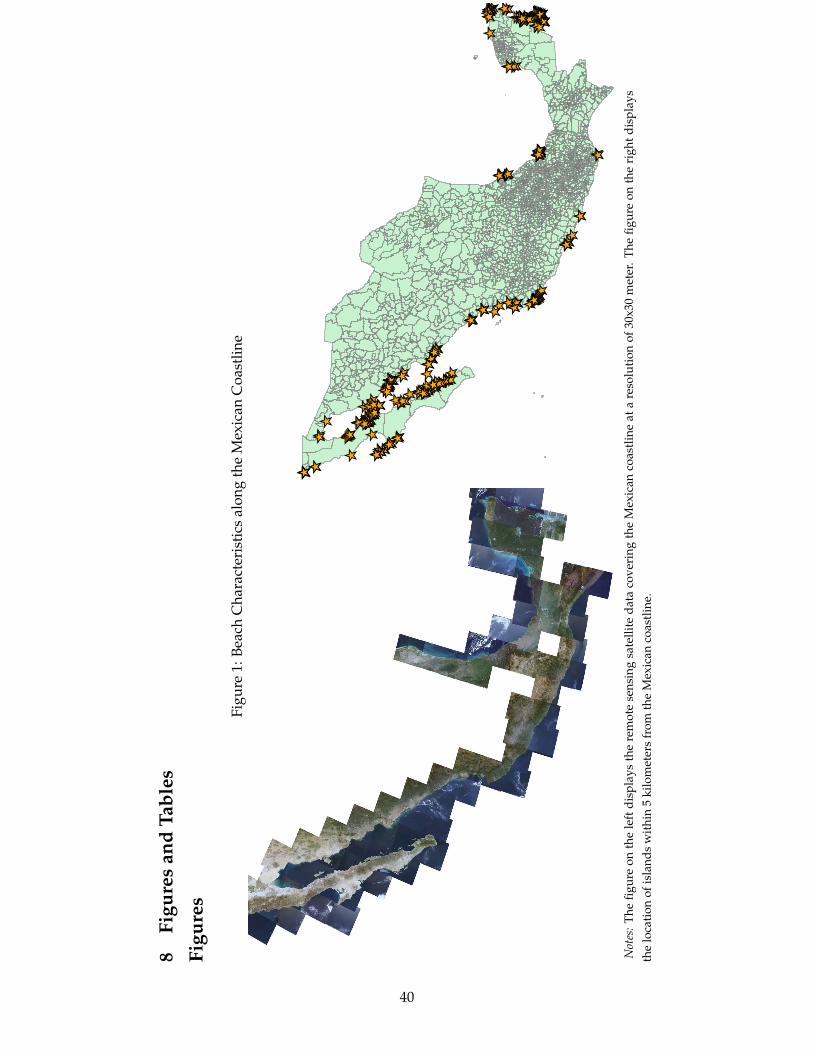
8Fi

gure

san

dTa

bles

Figu

res

Figu

re1:

Beac

hC

hara

cter

isti

csal

ong

the

Mex

ican

Coa

stlin

e

 

_

__ _

_ _ _

_

__ __ ___ _ _

_ _

____

__

_

_

_

__

__ ______ _ _______ _ _ __ __ ______ __ __ __ _ _ __ __ __ ____ ___ _ ____ __ __ ___ __ __ __ _ _ __ __ __ _ _ _______ __ __ _____ _

_

__

_ ____ __

_

__

_

_ _

_

_

_

_

_

_

_

_

_ _

_

_

_ _

_

_

__

_

_

__

_

_

_

_

_

_ _

_

_

_

_

_

__

_

_

_

__

__

_

_

_

_

_

__

_

_

_

___

_

__ _

_

_

_

_ _

____

_ _______ ______ ____ __ __ ___ _______ __ __

______ ____ __

__ __ ___ _ ____ __ _ __ __ _ _______ __ _ ___ ____ _

_ ___ __ __ ________ __ ___ _ ____ ____ _____ _ __

___ ______ ___ _ _____

____

_ __

_

_

_

_

_

_

_

_

_

_

_

___

_

_ _

__

_

__

_

Not

es:T

hefig

ure

onth

ele

ftdi

spla

ysth

ere

mot

ese

nsin

gsa

telli

teda

taco

veri

ngth

eM

exic

anco

astl

ine

ata

reso

luti

onof

30x3

0m

eter

.Th

efig

ure

onth

eri

ghtd

ispl

ays

the

loca

tion

ofis

land

sw

ithi

n5

kilo

met

ers

from

the

Mex

ican

coas

tlin

e.

40

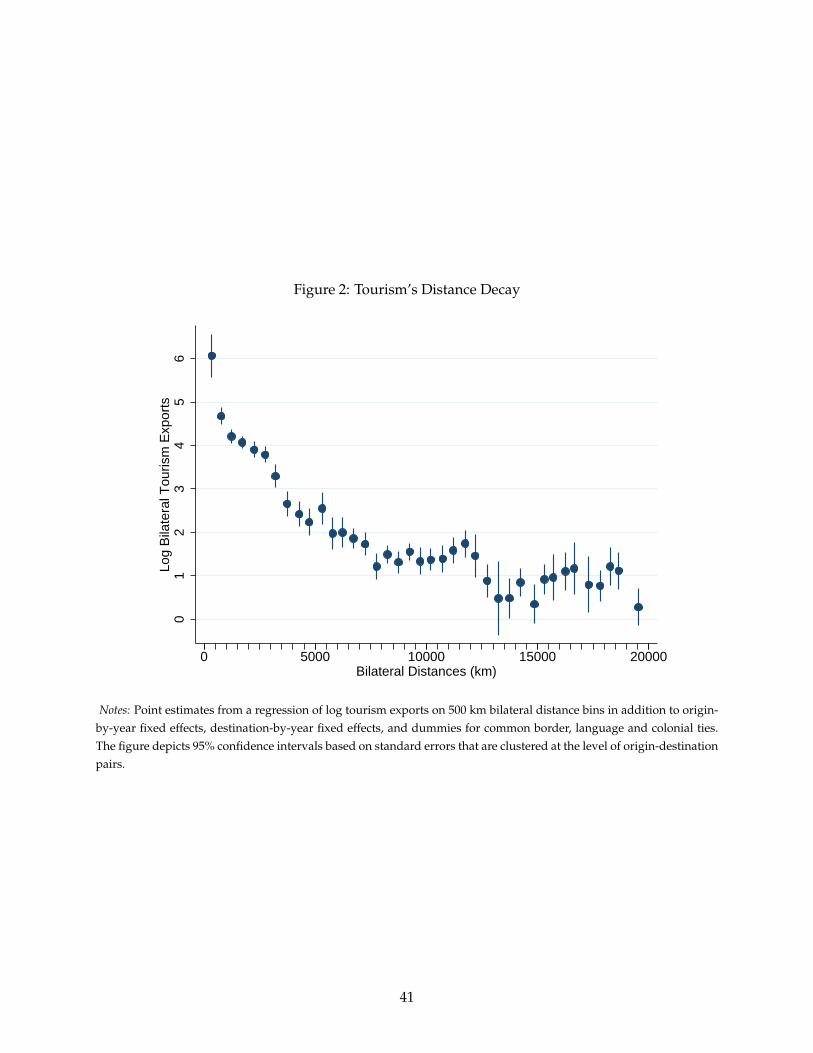
Figure 2: Tourism’s Distance Decay

01

23

45

6Lo

g B

ilate

ral T

ouris

m E

xpor

ts

0 5000 10000 15000 20000Bilateral Distances (km)

Notes: Point estimates from a regression of log tourism exports on 500 km bilateral distance bins in addition to origin-by-year fixed effects, destination-by-year fixed effects, and dummies for common border, language and colonial ties.The figure depicts 95% confidence intervals based on standard errors that are clustered at the level of origin-destinationpairs.

41

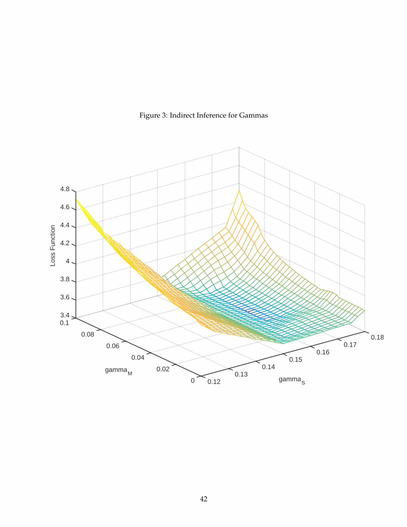
Figure 3: Indirect Inference for Gammas

0.180.17

0.16

gammaS

0.150.14

0.130.120

0.02

0.04

gammaM

0.06

0.08

3.4

3.6

3.8

4

4.2

4.4

4.6

4.8

0.1

Loss

Fun

ctio

n

42

Tables

Table 1: Beach Tourism in Mexico

Number of Municipalities

Sum of Hotel Revenues in 1998 and 2008 (Thousands of Pesos)

Share of National Hotel Revenues 1998 and 2008

Inland Municipalities 2305 46,070,000 0.365

Coastal Municipalities 150 80,130,000 0.635

Notes: The source are the Censos Economicos for 1998 and 2008.

43

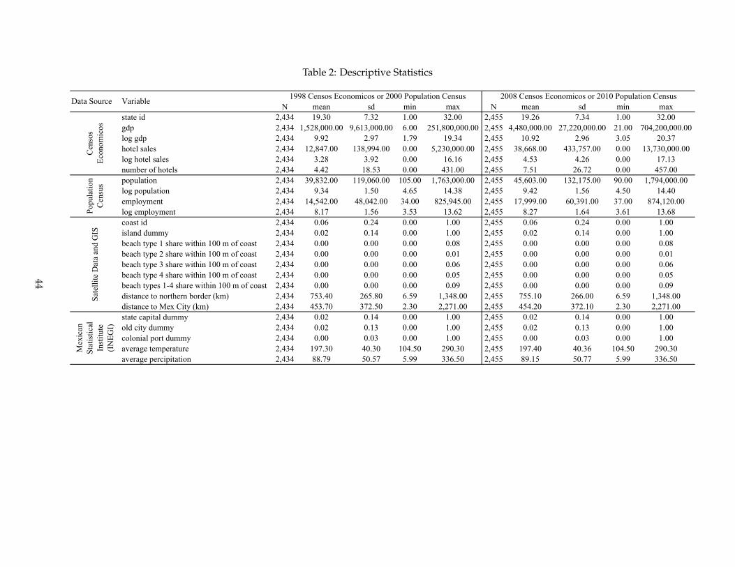
Table 2: Descriptive Statistics

N mean sd min max N mean sd min maxstate id 2,434 19.30 7.32 1.00 32.00 2,455 19.26 7.34 1.00 32.00gdp 2,434 1,528,000.00 9,613,000.00 6.00 251,800,000.00 2,455 4,480,000.00 27,220,000.00 21.00 704,200,000.00log gdp 2,434 9.92 2.97 1.79 19.34 2,455 10.92 2.96 3.05 20.37hotel sales 2,434 12,847.00 138,994.00 0.00 5,230,000.00 2,455 38,668.00 433,757.00 0.00 13,730,000.00log hotel sales 2,434 3.28 3.92 0.00 16.16 2,455 4.53 4.26 0.00 17.13number of hotels 2,434 4.42 18.53 0.00 431.00 2,455 7.51 26.72 0.00 457.00population 2,434 39,832.00 119,060.00 105.00 1,763,000.00 2,455 45,603.00 132,175.00 90.00 1,794,000.00log population 2,434 9.34 1.50 4.65 14.38 2,455 9.42 1.56 4.50 14.40employment 2,434 14,542.00 48,042.00 34.00 825,945.00 2,455 17,999.00 60,391.00 37.00 874,120.00log employment 2,434 8.17 1.56 3.53 13.62 2,455 8.27 1.64 3.61 13.68coast id 2,434 0.06 0.24 0.00 1.00 2,455 0.06 0.24 0.00 1.00island dummy 2,434 0.02 0.14 0.00 1.00 2,455 0.02 0.14 0.00 1.00beach type 1 share within 100 m of coast 2,434 0.00 0.00 0.00 0.08 2,455 0.00 0.00 0.00 0.08beach type 2 share within 100 m of coast 2,434 0.00 0.00 0.00 0.01 2,455 0.00 0.00 0.00 0.01beach type 3 share within 100 m of coast 2,434 0.00 0.00 0.00 0.06 2,455 0.00 0.00 0.00 0.06beach type 4 share within 100 m of coast 2,434 0.00 0.00 0.00 0.05 2,455 0.00 0.00 0.00 0.05beach types 1-4 share within 100 m of coast 2,434 0.00 0.00 0.00 0.09 2,455 0.00 0.00 0.00 0.09distance to northern border (km) 2,434 753.40 265.80 6.59 1,348.00 2,455 755.10 266.00 6.59 1,348.00distance to Mex City (km) 2,434 453.70 372.50 2.30 2,271.00 2,455 454.20 372.10 2.30 2,271.00state capital dummy 2,434 0.02 0.14 0.00 1.00 2,455 0.02 0.14 0.00 1.00old city dummy 2,434 0.02 0.13 0.00 1.00 2,455 0.02 0.13 0.00 1.00colonial port dummy 2,434 0.00 0.03 0.00 1.00 2,455 0.00 0.03 0.00 1.00average temperature 2,434 197.30 40.30 104.50 290.30 2,455 197.40 40.36 104.50 290.30average percipitation 2,434 88.79 50.57 5.99 336.50 2,455 89.15 50.77 5.99 336.50

Mex

ican

St

atis

tical

In

stitu

te

(IN

EGI)

VariableData SourceC

enso

s Ec

onom

icos

1998 Censos Economicos or 2000 Population Census 2008 Censos Economicos or 2010 Population CensusPo

pula

tion

Cen

sus

Sate

llite

Dat

a an

d G

IS

44

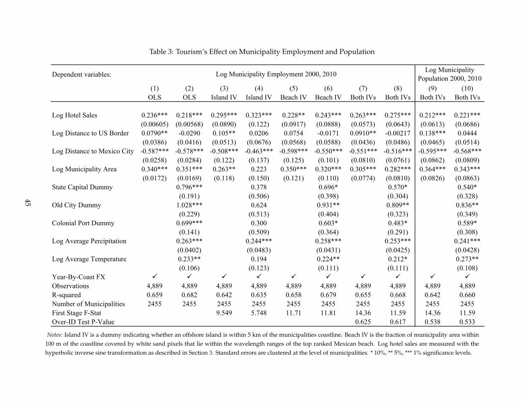
Table 3: Tourism’s Effect on Municipality Employment and Population

Dependent variables:

(1) (2) (3) (4) (5) (6) (7) (8) (9) (10)OLS OLS Island IV Island IV Beach IV Beach IV Both IVs Both IVs Both IVs Both IVs

Log Hotel Sales 0.236*** 0.218*** 0.295*** 0.323*** 0.228** 0.243*** 0.263*** 0.275*** 0.212*** 0.221***(0.00605) (0.00568) (0.0890) (0.122) (0.0917) (0.0888) (0.0573) (0.0643) (0.0613) (0.0686)

Log Distance to US Border 0.0790** -0.0290 0.105** 0.0206 0.0754 -0.0171 0.0910** -0.00217 0.138*** 0.0444(0.0386) (0.0416) (0.0513) (0.0676) (0.0568) (0.0588) (0.0436) (0.0486) (0.0465) (0.0514)

Log Distance to Mexico City -0.587*** -0.578*** -0.508*** -0.463*** -0.598*** -0.550*** -0.551*** -0.516*** -0.595*** -0.568***(0.0258) (0.0284) (0.122) (0.137) (0.125) (0.101) (0.0810) (0.0761) (0.0862) (0.0809)

Log Municipality Area 0.340*** 0.351*** 0.263** 0.223 0.350*** 0.320*** 0.305*** 0.282*** 0.364*** 0.343***(0.0172) (0.0169) (0.118) (0.150) (0.121) (0.110) (0.0774) (0.0810) (0.0826) (0.0863)

State Capital Dummy 0.796*** 0.378 0.696* 0.570* 0.540*(0.191) (0.506) (0.398) (0.304) (0.328)

Old City Dummy 1.028*** 0.624 0.931** 0.809** 0.836**(0.229) (0.513) (0.404) (0.323) (0.349)

Colonial Port Dummy 0.699*** 0.300 0.603* 0.483* 0.589*(0.141) (0.509) (0.364) (0.291) (0.308)

Log Average Percipitation 0.263*** 0.244*** 0.258*** 0.253*** 0.241***(0.0402) (0.0483) (0.0431) (0.0425) (0.0428)

Log Average Temperature 0.233** 0.194 0.224** 0.212* 0.273**(0.106) (0.123) (0.111) (0.111) (0.108)

Year-By-Coast FX Observations 4,889 4,889 4,889 4,889 4,889 4,889 4,889 4,889 4,889 4,889R-squared 0.659 0.682 0.642 0.635 0.658 0.679 0.655 0.668 0.642 0.660Number of Municipalities 2455 2455 2455 2455 2455 2455 2455 2455 2455 2455First Stage F-Stat 9.549 5.748 11.71 11.81 14.36 11.59 14.36 11.59Over-ID Test P-Value 0.625 0.617 0.538 0.533

Log Municipality Employment 2000, 2010 Log Municipality Population 2000, 2010

Notes: Island IV is a dummy indicating whether an offshore island is within 5 km of the municipalities coastline. Beach IV is the fraction of municipality area within100 m of the coastline covered by white sand pixels that lie within the wavelength ranges of the top ranked Mexican beach. Log hotel sales are measured with thehyperbolic inverse sine transformation as described in Section 3. Standard errors are clustered at the level of municipalities. * 10%, ** 5%, *** 1% significance levels.

45

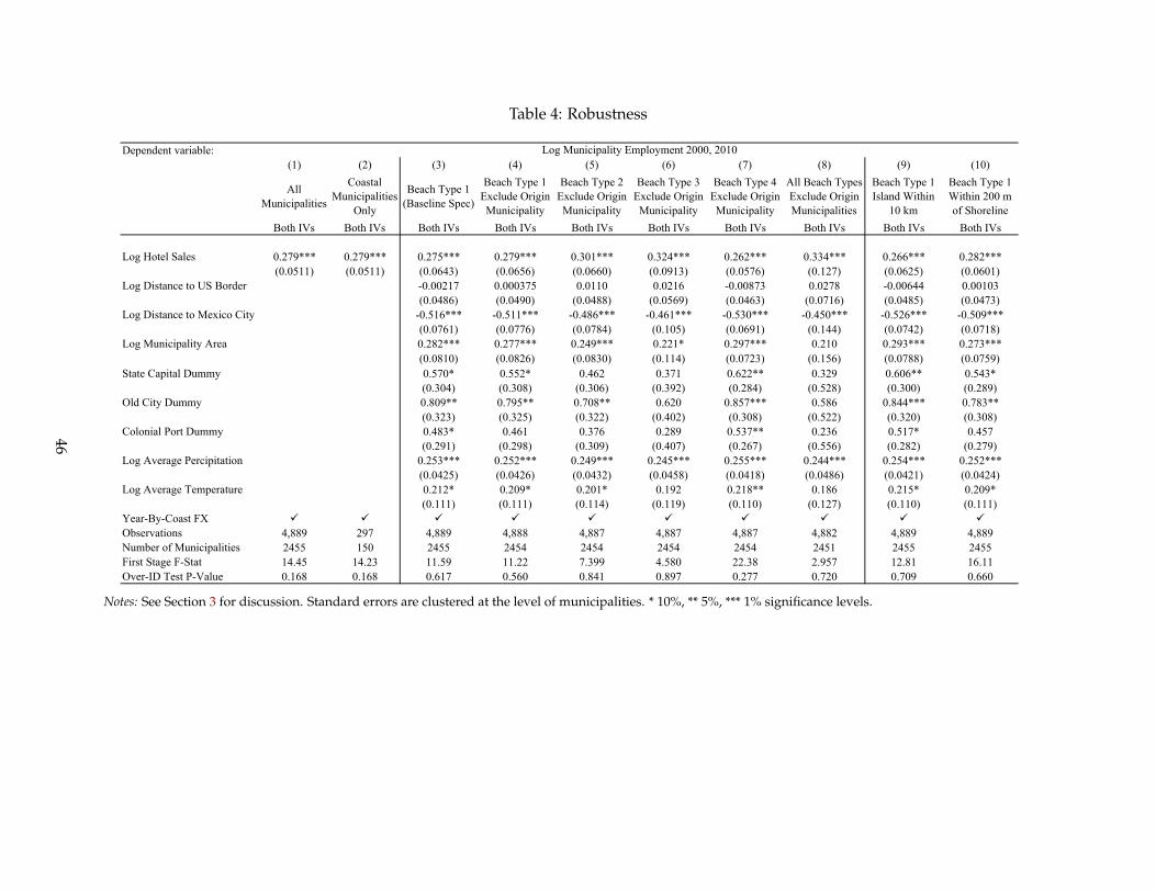
Table 4: Robustness

Dependent variable:(1) (2) (3) (4) (5) (6) (7) (8) (9) (10)

All Municipalities

Coastal Municipalities

Only

Beach Type 1 (Baseline Spec)

Beach Type 1 Exclude Origin Municipality

Beach Type 2 Exclude Origin Municipality

Beach Type 3 Exclude Origin Municipality

Beach Type 4 Exclude Origin Municipality

All Beach Types Exclude Origin Municipalities

Beach Type 1 Island Within

10 km

Beach Type 1 Within 200 m of Shoreline

Both IVs Both IVs Both IVs Both IVs Both IVs Both IVs Both IVs Both IVs Both IVs Both IVs

Log Hotel Sales 0.279*** 0.279*** 0.275*** 0.279*** 0.301*** 0.324*** 0.262*** 0.334*** 0.266*** 0.282***(0.0511) (0.0511) (0.0643) (0.0656) (0.0660) (0.0913) (0.0576) (0.127) (0.0625) (0.0601)

Log Distance to US Border -0.00217 0.000375 0.0110 0.0216 -0.00873 0.0278 -0.00644 0.00103(0.0486) (0.0490) (0.0488) (0.0569) (0.0463) (0.0716) (0.0485) (0.0473)

Log Distance to Mexico City -0.516*** -0.511*** -0.486*** -0.461*** -0.530*** -0.450*** -0.526*** -0.509***(0.0761) (0.0776) (0.0784) (0.105) (0.0691) (0.144) (0.0742) (0.0718)

Log Municipality Area 0.282*** 0.277*** 0.249*** 0.221* 0.297*** 0.210 0.293*** 0.273***(0.0810) (0.0826) (0.0830) (0.114) (0.0723) (0.156) (0.0788) (0.0759)

State Capital Dummy 0.570* 0.552* 0.462 0.371 0.622** 0.329 0.606** 0.543*(0.304) (0.308) (0.306) (0.392) (0.284) (0.528) (0.300) (0.289)

Old City Dummy 0.809** 0.795** 0.708** 0.620 0.857*** 0.586 0.844*** 0.783**(0.323) (0.325) (0.322) (0.402) (0.308) (0.522) (0.320) (0.308)

Colonial Port Dummy 0.483* 0.461 0.376 0.289 0.537** 0.236 0.517* 0.457(0.291) (0.298) (0.309) (0.407) (0.267) (0.556) (0.282) (0.279)

Log Average Percipitation 0.253*** 0.252*** 0.249*** 0.245*** 0.255*** 0.244*** 0.254*** 0.252***(0.0425) (0.0426) (0.0432) (0.0458) (0.0418) (0.0486) (0.0421) (0.0424)

Log Average Temperature 0.212* 0.209* 0.201* 0.192 0.218** 0.186 0.215* 0.209*(0.111) (0.111) (0.114) (0.119) (0.110) (0.127) (0.110) (0.111)

Year-By-Coast FX Observations 4,889 297 4,889 4,888 4,887 4,887 4,887 4,882 4,889 4,889Number of Municipalities 2455 150 2455 2454 2454 2454 2454 2451 2455 2455First Stage F-Stat 14.45 14.23 11.59 11.22 7.399 4.580 22.38 2.957 12.81 16.11Over-ID Test P-Value 0.168 0.168 0.617 0.560 0.841 0.897 0.277 0.720 0.709 0.660

Log Municipality Employment 2000, 2010

Notes: See Section 3 for discussion. Standard errors are clustered at the level of municipalities. * 10%, ** 5%, *** 1% significance levels.

46

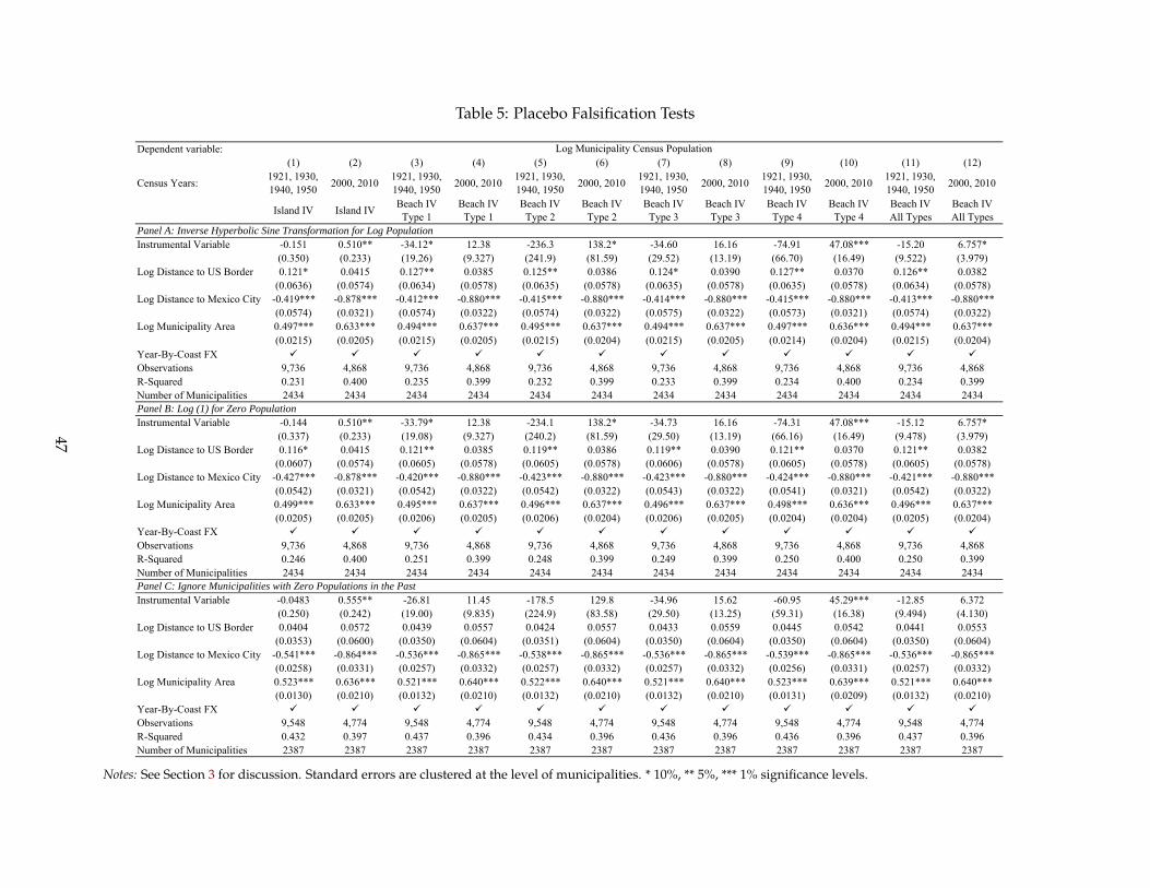
Table 5: Placebo Falsification Tests

Dependent variable:(1) (2) (3) (4) (5) (6) (7) (8) (9) (10) (11) (12)

Census Years: 1921, 1930, 1940, 1950 2000, 2010 1921, 1930,

1940, 1950 2000, 2010 1921, 1930, 1940, 1950 2000, 2010 1921, 1930,

1940, 1950 2000, 2010 1921, 1930, 1940, 1950 2000, 2010 1921, 1930,

1940, 1950 2000, 2010

Island IV Island IV Beach IV Type 1

Beach IV Type 1

Beach IV Type 2

Beach IV Type 2

Beach IV Type 3

Beach IV Type 3

Beach IV Type 4

Beach IV Type 4

Beach IV All Types

Beach IV All Types

Instrumental Variable -0.151 0.510** -34.12* 12.38 -236.3 138.2* -34.60 16.16 -74.91 47.08*** -15.20 6.757*(0.350) (0.233) (19.26) (9.327) (241.9) (81.59) (29.52) (13.19) (66.70) (16.49) (9.522) (3.979)

Log Distance to US Border 0.121* 0.0415 0.127** 0.0385 0.125** 0.0386 0.124* 0.0390 0.127** 0.0370 0.126** 0.0382(0.0636) (0.0574) (0.0634) (0.0578) (0.0635) (0.0578) (0.0635) (0.0578) (0.0635) (0.0578) (0.0634) (0.0578)

Log Distance to Mexico City -0.419*** -0.878*** -0.412*** -0.880*** -0.415*** -0.880*** -0.414*** -0.880*** -0.415*** -0.880*** -0.413*** -0.880***(0.0574) (0.0321) (0.0574) (0.0322) (0.0574) (0.0322) (0.0575) (0.0322) (0.0573) (0.0321) (0.0574) (0.0322)

Log Municipality Area 0.497*** 0.633*** 0.494*** 0.637*** 0.495*** 0.637*** 0.494*** 0.637*** 0.497*** 0.636*** 0.494*** 0.637***(0.0215) (0.0205) (0.0215) (0.0205) (0.0215) (0.0204) (0.0215) (0.0205) (0.0214) (0.0204) (0.0215) (0.0204)

Year-By-Coast FX Observations 9,736 4,868 9,736 4,868 9,736 4,868 9,736 4,868 9,736 4,868 9,736 4,868R-Squared 0.231 0.400 0.235 0.399 0.232 0.399 0.233 0.399 0.234 0.400 0.234 0.399Number of Municipalities 2434 2434 2434 2434 2434 2434 2434 2434 2434 2434 2434 2434

Instrumental Variable -0.144 0.510** -33.79* 12.38 -234.1 138.2* -34.73 16.16 -74.31 47.08*** -15.12 6.757*(0.337) (0.233) (19.08) (9.327) (240.2) (81.59) (29.50) (13.19) (66.16) (16.49) (9.478) (3.979)

Log Distance to US Border 0.116* 0.0415 0.121** 0.0385 0.119** 0.0386 0.119** 0.0390 0.121** 0.0370 0.121** 0.0382(0.0607) (0.0574) (0.0605) (0.0578) (0.0605) (0.0578) (0.0606) (0.0578) (0.0605) (0.0578) (0.0605) (0.0578)

Log Distance to Mexico City -0.427*** -0.878*** -0.420*** -0.880*** -0.423*** -0.880*** -0.423*** -0.880*** -0.424*** -0.880*** -0.421*** -0.880***(0.0542) (0.0321) (0.0542) (0.0322) (0.0542) (0.0322) (0.0543) (0.0322) (0.0541) (0.0321) (0.0542) (0.0322)

Log Municipality Area 0.499*** 0.633*** 0.495*** 0.637*** 0.496*** 0.637*** 0.496*** 0.637*** 0.498*** 0.636*** 0.496*** 0.637***(0.0205) (0.0205) (0.0206) (0.0205) (0.0206) (0.0204) (0.0206) (0.0205) (0.0204) (0.0204) (0.0205) (0.0204)

Year-By-Coast FX Observations 9,736 4,868 9,736 4,868 9,736 4,868 9,736 4,868 9,736 4,868 9,736 4,868R-Squared 0.246 0.400 0.251 0.399 0.248 0.399 0.249 0.399 0.250 0.400 0.250 0.399Number of Municipalities 2434 2434 2434 2434 2434 2434 2434 2434 2434 2434 2434 2434

Instrumental Variable -0.0483 0.555** -26.81 11.45 -178.5 129.8 -34.96 15.62 -60.95 45.29*** -12.85 6.372(0.250) (0.242) (19.00) (9.835) (224.9) (83.58) (29.50) (13.25) (59.31) (16.38) (9.494) (4.130)

Log Distance to US Border 0.0404 0.0572 0.0439 0.0557 0.0424 0.0557 0.0433 0.0559 0.0445 0.0542 0.0441 0.0553(0.0353) (0.0600) (0.0350) (0.0604) (0.0351) (0.0604) (0.0350) (0.0604) (0.0350) (0.0604) (0.0350) (0.0604)

Log Distance to Mexico City -0.541*** -0.864*** -0.536*** -0.865*** -0.538*** -0.865*** -0.536*** -0.865*** -0.539*** -0.865*** -0.536*** -0.865***(0.0258) (0.0331) (0.0257) (0.0332) (0.0257) (0.0332) (0.0257) (0.0332) (0.0256) (0.0331) (0.0257) (0.0332)

Log Municipality Area 0.523*** 0.636*** 0.521*** 0.640*** 0.522*** 0.640*** 0.521*** 0.640*** 0.523*** 0.639*** 0.521*** 0.640***(0.0130) (0.0210) (0.0132) (0.0210) (0.0132) (0.0210) (0.0132) (0.0210) (0.0131) (0.0209) (0.0132) (0.0210)

Year-By-Coast FX Observations 9,548 4,774 9,548 4,774 9,548 4,774 9,548 4,774 9,548 4,774 9,548 4,774R-Squared 0.432 0.397 0.437 0.396 0.434 0.396 0.436 0.396 0.436 0.396 0.437 0.396Number of Municipalities 2387 2387 2387 2387 2387 2387 2387 2387 2387 2387 2387 2387

Log Municipality Census Population

Panel A: Inverse Hyperbolic Sine Transformation for Log Population

Panel B: Log (1) for Zero Population

Panel C: Ignore Municipalities with Zero Populations in the Past

Notes: See Section 3 for discussion. Standard errors are clustered at the level of municipalities. * 10%, ** 5%, *** 1% significance levels.

47

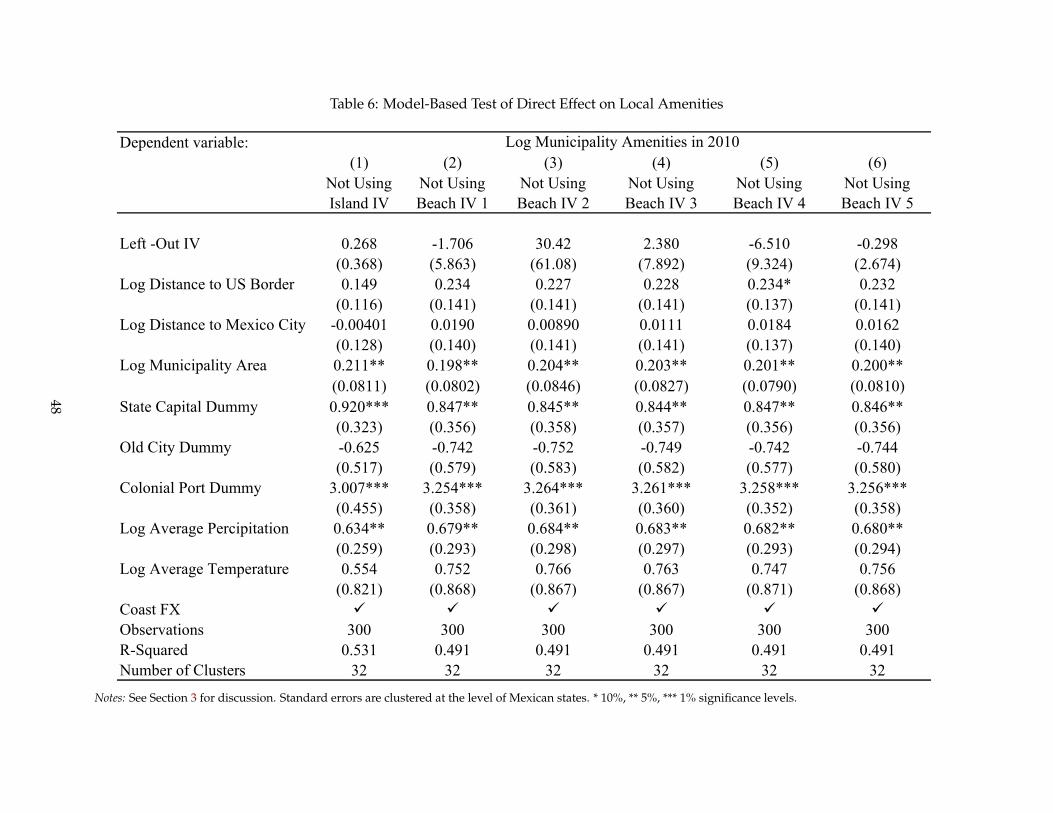
Table 6: Model-Based Test of Direct Effect on Local Amenities

Dependent variable:(1) (2) (3) (4) (5) (6)

Not Using Island IV

Not Using Beach IV 1

Not Using Beach IV 2

Not Using Beach IV 3

Not Using Beach IV 4

Not Using Beach IV 5

Left -Out IV 0.268 -1.706 30.42 2.380 -6.510 -0.298(0.368) (5.863) (61.08) (7.892) (9.324) (2.674)

Log Distance to US Border 0.149 0.234 0.227 0.228 0.234* 0.232(0.116) (0.141) (0.141) (0.141) (0.137) (0.141)

Log Distance to Mexico City -0.00401 0.0190 0.00890 0.0111 0.0184 0.0162(0.128) (0.140) (0.141) (0.141) (0.137) (0.140)

Log Municipality Area 0.211** 0.198** 0.204** 0.203** 0.201** 0.200**(0.0811) (0.0802) (0.0846) (0.0827) (0.0790) (0.0810)

State Capital Dummy 0.920*** 0.847** 0.845** 0.844** 0.847** 0.846**(0.323) (0.356) (0.358) (0.357) (0.356) (0.356)

Old City Dummy -0.625 -0.742 -0.752 -0.749 -0.742 -0.744(0.517) (0.579) (0.583) (0.582) (0.577) (0.580)

Colonial Port Dummy 3.007*** 3.254*** 3.264*** 3.261*** 3.258*** 3.256***(0.455) (0.358) (0.361) (0.360) (0.352) (0.358)

Log Average Percipitation 0.634** 0.679** 0.684** 0.683** 0.682** 0.680**(0.259) (0.293) (0.298) (0.297) (0.293) (0.294)

Log Average Temperature 0.554 0.752 0.766 0.763 0.747 0.756(0.821) (0.868) (0.867) (0.867) (0.871) (0.868)

Coast FX Observations 300 300 300 300 300 300R-Squared 0.531 0.491 0.491 0.491 0.491 0.491Number of Clusters 32 32 32 32 32 32

Log Municipality Amenities in 2010

Notes: See Section 3 for discussion. Standard errors are clustered at the level of Mexican states. * 10%, ** 5%, *** 1% significance levels.

48

Table 7: Tourism’s Effect on Municipality Employment by Group

(1) (2) (3) (4) (5) (6) (7) (8)Dependent VariableGender Male Male Male Male Female Female Female FemaleEducation Skilled Skilled Unskilled Unskilled Skilled Skilled Unskilled UnskilledEthnicity Hispanic Indigenous Hispanic Indigenous Hispanic Indigenous Hispanic IndigenousSpecification Both IVs Both IVs Both IVs Both IVs Both IVs Both IVs Both IVs Both IVs

Log Hotel Sales 0.296*** 0.710*** 0.0796 0.616*** 0.349*** 0.660*** 0.153* 0.605***(0.0739) (0.197) (0.0845) (0.204) (0.0771) (0.186) (0.0878) (0.190)

Log Distance to US Border -0.223*** 0.438*** -0.111* 0.675*** -0.152** 0.463*** 0.0530 0.647***(0.0578) (0.129) (0.0666) (0.132) (0.0593) (0.125) (0.0694) (0.125)

Log Distance to Mexico City -0.954*** 0.513** -1.153*** 0.563** -0.901*** 0.529** -1.128*** 0.514**(0.0892) (0.227) (0.102) (0.235) (0.0922) (0.214) (0.104) (0.220)

Log Municipality Area 0.407*** -0.649*** 0.761*** -0.552** 0.330*** -0.650*** 0.567*** -0.656***(0.0933) (0.244) (0.106) (0.253) (0.0975) (0.231) (0.110) (0.236)

State Capital Dummy 0.705* -0.200 0.520 -0.420 0.782** 0.229 0.669 0.0478(0.370) (0.902) (0.457) (0.948) (0.379) (0.855) (0.467) (0.893)

Old City Dummy 0.773** -0.533 1.145** -0.514 0.663* -0.202 1.112** -0.103(0.379) (0.926) (0.478) (0.979) (0.387) (0.865) (0.493) (0.918)

Colonial Port Dummy 0.720* -1.790** 1.067*** -1.971** 0.788* -0.967 1.255*** -1.128(0.391) (0.844) (0.405) (0.871) (0.435) (0.805) (0.399) (0.864)

Log Average Percipitation -0.515*** 1.473*** -0.500*** 1.954*** -0.605*** 1.182*** -0.708*** 1.572***(0.0674) (0.128) (0.0819) (0.135) (0.0644) (0.122) (0.0790) (0.130)

Log Average Temperature 1.094*** 0.00335 1.051*** -0.176 0.947*** -0.133 0.949*** -0.408(0.158) (0.310) (0.193) (0.322) (0.152) (0.294) (0.180) (0.314)

Year-By-Coast FX Observations 4,889 4,889 4,889 4,889 4,889 4,889 4,889 4,889Number of Municipalities 2455 2455 2455 2455 2455 2455 2455 2455First Stage F-Stat 11.59 11.59 11.59 11.59 11.59 11.59 11.59 11.59Over-ID Test P-Value 0.176 0.566 0.0593 0.504 0.350 0.509 0.213 0.611

Log Employment by Group 2000, 2010

Notes: See Section 3 for discussion. Standard errors are clustered at the level of municipalities. * 10%, ** 5%, *** 1% significance levels.

49

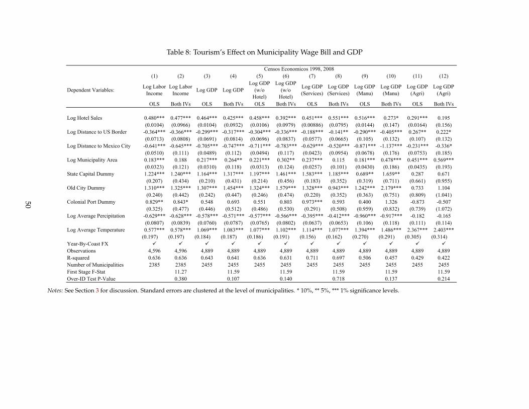
Table 8: Tourism’s Effect on Municipality Wage Bill and GDP

(1) (2) (3) (4) (5) (6) (7) (8) (9) (10) (11) (12)

Dependent Variables: Log Labor Income

Log Labor Income Log GDP Log GDP

Log GDP (w/o

Hotel)

Log GDP (w/o

Hotel)

Log GDP (Services)

Log GDP (Services)

Log GDP (Manu)

Log GDP (Manu)

Log GDP (Agri)

Log GDP (Agri)

OLS Both IVs OLS Both IVs OLS Both IVs OLS Both IVs OLS Both IVs OLS Both IVs

Log Hotel Sales 0.480*** 0.477*** 0.464*** 0.425*** 0.458*** 0.392*** 0.451*** 0.551*** 0.516*** 0.273* 0.291*** 0.195(0.0104) (0.0966) (0.0104) (0.0932) (0.0106) (0.0979) (0.00886) (0.0795) (0.0144) (0.147) (0.0164) (0.156)

Log Distance to US Border -0.364*** -0.366*** -0.299*** -0.317*** -0.304*** -0.336*** -0.188*** -0.141** -0.290*** -0.405*** 0.267** 0.222*(0.0713) (0.0808) (0.0691) (0.0814) (0.0696) (0.0837) (0.0577) (0.0665) (0.105) (0.132) (0.107) (0.132)

Log Distance to Mexico City -0.641*** -0.645*** -0.705*** -0.747*** -0.711*** -0.783*** -0.629*** -0.520*** -0.871*** -1.137*** -0.231*** -0.336*(0.0510) (0.111) (0.0489) (0.112) (0.0494) (0.117) (0.0423) (0.0954) (0.0678) (0.176) (0.0753) (0.185)

Log Municipality Area 0.183*** 0.188 0.217*** 0.264** 0.221*** 0.302** 0.237*** 0.115 0.181*** 0.478*** 0.451*** 0.569***(0.0323) (0.121) (0.0310) (0.118) (0.0313) (0.124) (0.0257) (0.101) (0.0430) (0.186) (0.0435) (0.193)

State Capital Dummy 1.224*** 1.240*** 1.164*** 1.317*** 1.197*** 1.461*** 1.583*** 1.185*** 0.689** 1.659** 0.287 0.671(0.207) (0.434) (0.210) (0.431) (0.214) (0.456) (0.183) (0.352) (0.319) (0.711) (0.661) (0.955)

Old City Dummy 1.310*** 1.325*** 1.307*** 1.454*** 1.324*** 1.579*** 1.328*** 0.943*** 1.242*** 2.179*** 0.733 1.104(0.240) (0.442) (0.242) (0.447) (0.246) (0.474) (0.220) (0.352) (0.363) (0.751) (0.809) (1.041)

Colonial Port Dummy 0.829** 0.843* 0.548 0.693 0.551 0.803 0.973*** 0.593 0.400 1.326 -0.873 -0.507(0.325) (0.477) (0.446) (0.512) (0.486) (0.530) (0.291) (0.508) (0.959) (0.832) (0.739) (1.072)

Log Average Percipitation -0.629*** -0.628*** -0.578*** -0.571*** -0.577*** -0.566*** -0.395*** -0.412*** -0.960*** -0.917*** -0.182 -0.165(0.0807) (0.0839) (0.0760) (0.0787) (0.0765) (0.0802) (0.0637) (0.0653) (0.106) (0.118) (0.111) (0.114)

Log Average Temperature 0.577*** 0.578*** 1.069*** 1.083*** 1.077*** 1.102*** 1.114*** 1.077*** 1.394*** 1.486*** 2.367*** 2.403***(0.197) (0.197) (0.184) (0.187) (0.186) (0.191) (0.156) (0.162) (0.270) (0.291) (0.305) (0.314)

Year-By-Coast FX Observations 4,596 4,596 4,889 4,889 4,889 4,889 4,889 4,889 4,889 4,889 4,889 4,889R-squared 0.636 0.636 0.643 0.641 0.636 0.631 0.711 0.697 0.506 0.457 0.429 0.422Number of Municipalities 2385 2385 2455 2455 2455 2455 2455 2455 2455 2455 2455 2455First Stage F-Stat 11.27 11.59 11.59 11.59 11.59 11.59Over-ID Test P-Value 0.380 0.107 0.140 0.718 0.137 0.214

Censos Economicos 1998, 2008

Notes: See Section 3 for discussion. Standard errors are clustered at the level of municipalities. * 10%, ** 5%, *** 1% significance levels.

50

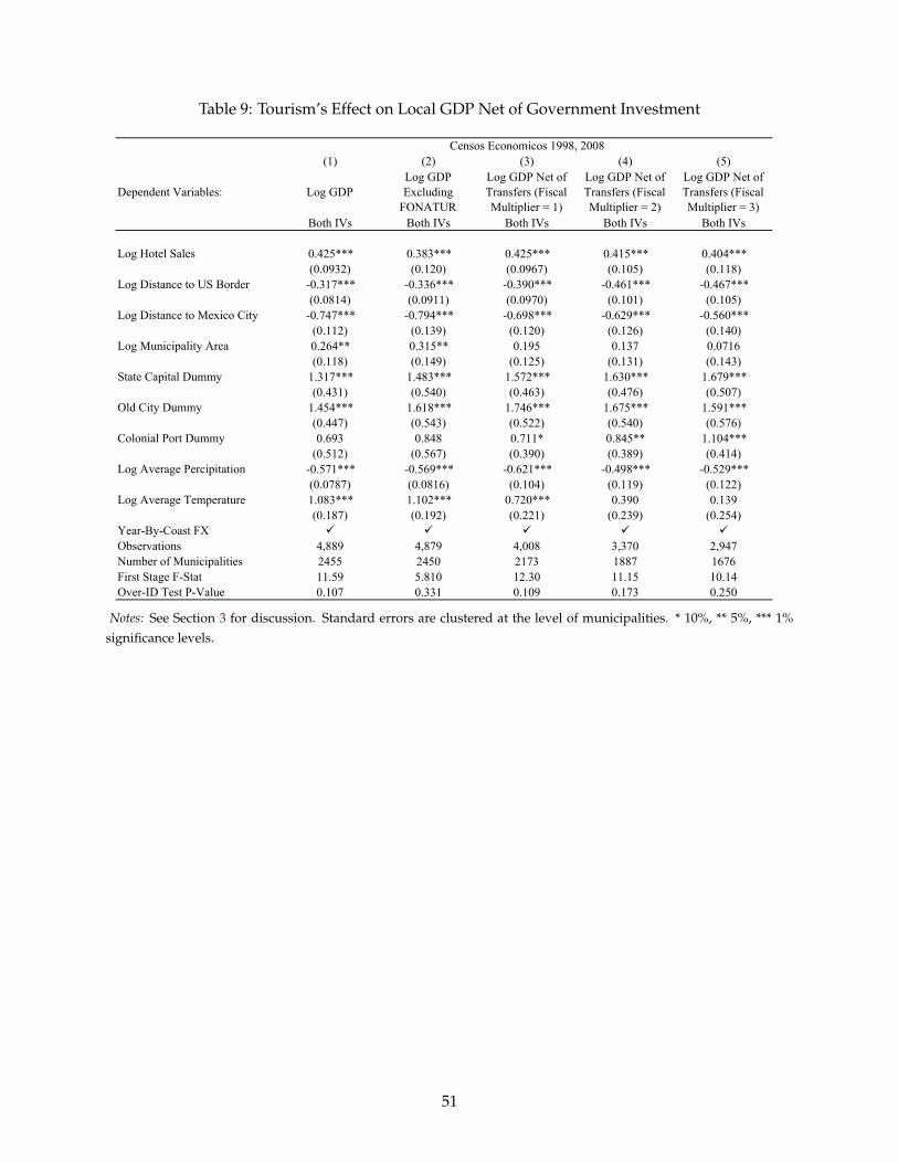
Table 9: Tourism’s Effect on Local GDP Net of Government Investment

(1) (2) (3) (4) (5)

Dependent Variables: Log GDPLog GDP Excluding

FONATUR

Log GDP Net of Transfers (Fiscal Multiplier = 1)

Log GDP Net of Transfers (Fiscal Multiplier = 2)

Log GDP Net of Transfers (Fiscal Multiplier = 3)

Both IVs Both IVs Both IVs Both IVs Both IVs

Log Hotel Sales 0.425*** 0.383*** 0.425*** 0.415*** 0.404***(0.0932) (0.120) (0.0967) (0.105) (0.118)

Log Distance to US Border -0.317*** -0.336*** -0.390*** -0.461*** -0.467***(0.0814) (0.0911) (0.0970) (0.101) (0.105)

Log Distance to Mexico City -0.747*** -0.794*** -0.698*** -0.629*** -0.560***(0.112) (0.139) (0.120) (0.126) (0.140)

Log Municipality Area 0.264** 0.315** 0.195 0.137 0.0716(0.118) (0.149) (0.125) (0.131) (0.143)

State Capital Dummy 1.317*** 1.483*** 1.572*** 1.630*** 1.679***(0.431) (0.540) (0.463) (0.476) (0.507)

Old City Dummy 1.454*** 1.618*** 1.746*** 1.675*** 1.591***(0.447) (0.543) (0.522) (0.540) (0.576)

Colonial Port Dummy 0.693 0.848 0.711* 0.845** 1.104***(0.512) (0.567) (0.390) (0.389) (0.414)

Log Average Percipitation -0.571*** -0.569*** -0.621*** -0.498*** -0.529***(0.0787) (0.0816) (0.104) (0.119) (0.122)

Log Average Temperature 1.083*** 1.102*** 0.720*** 0.390 0.139(0.187) (0.192) (0.221) (0.239) (0.254)

Year-By-Coast FX Observations 4,889 4,879 4,008 3,370 2,947Number of Municipalities 2455 2450 2173 1887 1676First Stage F-Stat 11.59 5.810 12.30 11.15 10.14Over-ID Test P-Value 0.107 0.331 0.109 0.173 0.250

Censos Economicos 1998, 2008

Notes: See Section 3 for discussion. Standard errors are clustered at the level of municipalities. * 10%, ** 5%, *** 1%significance levels.

51

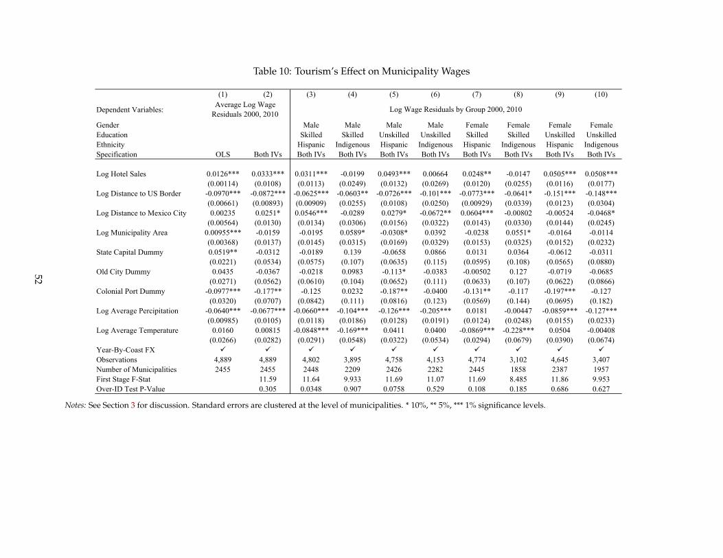
Table 10: Tourism’s Effect on Municipality Wages

(1) (2) (3) (4) (5) (6) (7) (8) (9) (10)

Dependent Variables:

Gender Male Male Male Male Female Female Female FemaleEducation Skilled Skilled Unskilled Unskilled Skilled Skilled Unskilled UnskilledEthnicity Hispanic Indigenous Hispanic Indigenous Hispanic Indigenous Hispanic IndigenousSpecification OLS Both IVs Both IVs Both IVs Both IVs Both IVs Both IVs Both IVs Both IVs Both IVs

Log Hotel Sales 0.0126*** 0.0333*** 0.0311*** -0.0199 0.0493*** 0.00664 0.0248** -0.0147 0.0505*** 0.0508***(0.00114) (0.0108) (0.0113) (0.0249) (0.0132) (0.0269) (0.0120) (0.0255) (0.0116) (0.0177)

Log Distance to US Border -0.0970*** -0.0872*** -0.0625*** -0.0603** -0.0726*** -0.101*** -0.0773*** -0.0641* -0.151*** -0.148***(0.00661) (0.00893) (0.00909) (0.0255) (0.0108) (0.0250) (0.00929) (0.0339) (0.0123) (0.0304)

Log Distance to Mexico City 0.00235 0.0251* 0.0546*** -0.0289 0.0279* -0.0672** 0.0604*** -0.00802 -0.00524 -0.0468*(0.00564) (0.0130) (0.0134) (0.0306) (0.0156) (0.0322) (0.0143) (0.0330) (0.0144) (0.0245)

Log Municipality Area 0.00955*** -0.0159 -0.0195 0.0589* -0.0308* 0.0392 -0.0238 0.0551* -0.0164 -0.0114(0.00368) (0.0137) (0.0145) (0.0315) (0.0169) (0.0329) (0.0153) (0.0325) (0.0152) (0.0232)

State Capital Dummy 0.0519** -0.0312 -0.0189 0.139 -0.0658 0.0866 0.0131 0.0364 -0.0612 -0.0311(0.0221) (0.0534) (0.0575) (0.107) (0.0635) (0.115) (0.0595) (0.108) (0.0565) (0.0880)

Old City Dummy 0.0435 -0.0367 -0.0218 0.0983 -0.113* -0.0383 -0.00502 0.127 -0.0719 -0.0685(0.0271) (0.0562) (0.0610) (0.104) (0.0652) (0.111) (0.0633) (0.107) (0.0622) (0.0866)

Colonial Port Dummy -0.0977*** -0.177** -0.125 0.0232 -0.187** -0.0400 -0.131** -0.117 -0.197*** -0.127(0.0320) (0.0707) (0.0842) (0.111) (0.0816) (0.123) (0.0569) (0.144) (0.0695) (0.182)

Log Average Percipitation -0.0640*** -0.0677*** -0.0660*** -0.104*** -0.126*** -0.205*** 0.0181 -0.00447 -0.0859*** -0.127***(0.00985) (0.0105) (0.0118) (0.0186) (0.0128) (0.0191) (0.0124) (0.0248) (0.0155) (0.0233)

Log Average Temperature 0.0160 0.00815 -0.0848*** -0.169*** 0.0411 0.0400 -0.0869*** -0.228*** 0.0504 -0.00408(0.0266) (0.0282) (0.0291) (0.0548) (0.0322) (0.0534) (0.0294) (0.0679) (0.0390) (0.0674)

Year-By-Coast FX Observations 4,889 4,889 4,802 3,895 4,758 4,153 4,774 3,102 4,645 3,407Number of Municipalities 2455 2455 2448 2209 2426 2282 2445 1858 2387 1957First Stage F-Stat 11.59 11.64 9.933 11.69 11.07 11.69 8.485 11.86 9.953Over-ID Test P-Value 0.305 0.0348 0.907 0.0758 0.529 0.108 0.185 0.686 0.627

Log Wage Residuals by Group 2000, 2010Average Log Wage Residuals 2000, 2010

Notes: See Section 3 for discussion. Standard errors are clustered at the level of municipalities. * 10%, ** 5%, *** 1% significance levels.

52

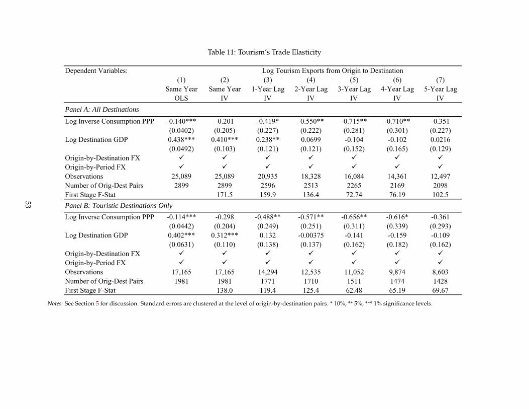
Table 11: Tourism’s Trade Elasticity

Dependent Variables:(1) (2) (3) (4) (5) (6) (7)

Same Year Same Year 1-Year Lag 2-Year Lag 3-Year Lag 4-Year Lag 5-Year LagOLS IV IV IV IV IV IV

Log Inverse Consumption PPP -0.140*** -0.201 -0.419* -0.550** -0.715** -0.710** -0.351(0.0402) (0.205) (0.227) (0.222) (0.281) (0.301) (0.227)

Log Destination GDP 0.438*** 0.410*** 0.238** 0.0699 -0.104 -0.102 0.0216(0.0492) (0.103) (0.121) (0.121) (0.152) (0.165) (0.129)

Origin-by-Destination FX Origin-by-Period FX Observations 25,089 25,089 20,935 18,328 16,084 14,361 12,497Number of Orig-Dest Pairs 2899 2899 2596 2513 2265 2169 2098First Stage F-Stat 171.5 159.9 136.4 72.74 76.19 102.5

Log Inverse Consumption PPP -0.114*** -0.298 -0.488** -0.571** -0.656** -0.616* -0.361(0.0442) (0.204) (0.249) (0.251) (0.311) (0.339) (0.293)

Log Destination GDP 0.402*** 0.312*** 0.132 -0.00375 -0.141 -0.159 -0.109(0.0631) (0.110) (0.138) (0.137) (0.162) (0.182) (0.162)

Origin-by-Destination FX Origin-by-Period FX Observations 17,165 17,165 14,294 12,535 11,052 9,874 8,603Number of Orig-Dest Pairs 1981 1981 1771 1710 1511 1474 1428First Stage F-Stat 138.0 119.4 125.4 62.48 65.19 69.67

Panel B: Touristic Destinations Only

Panel A: All Destinations

Log Tourism Exports from Origin to Destination

Notes: See Section 5 for discussion. Standard errors are clustered at the level of origin-by-destination pairs. * 10%, ** 5%, *** 1% significance levels.

53

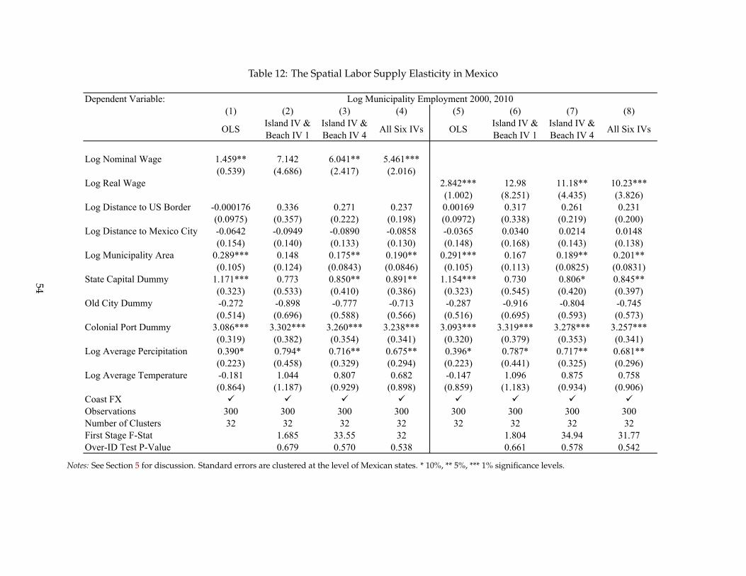
Table 12: The Spatial Labor Supply Elasticity in Mexico

Dependent Variable:(1) (2) (3) (4) (5) (6) (7) (8)

OLS Island IV & Beach IV 1

Island IV & Beach IV 4 All Six IVs OLS Island IV &

Beach IV 1Island IV & Beach IV 4 All Six IVs

Log Nominal Wage 1.459** 7.142 6.041** 5.461***(0.539) (4.686) (2.417) (2.016)

Log Real Wage 2.842*** 12.98 11.18** 10.23***(1.002) (8.251) (4.435) (3.826)

Log Distance to US Border -0.000176 0.336 0.271 0.237 0.00169 0.317 0.261 0.231(0.0975) (0.357) (0.222) (0.198) (0.0972) (0.338) (0.219) (0.200)

Log Distance to Mexico City -0.0642 -0.0949 -0.0890 -0.0858 -0.0365 0.0340 0.0214 0.0148(0.154) (0.140) (0.133) (0.130) (0.148) (0.168) (0.143) (0.138)

Log Municipality Area 0.289*** 0.148 0.175** 0.190** 0.291*** 0.167 0.189** 0.201**(0.105) (0.124) (0.0843) (0.0846) (0.105) (0.113) (0.0825) (0.0831)

State Capital Dummy 1.171*** 0.773 0.850** 0.891** 1.154*** 0.730 0.806* 0.845**(0.323) (0.533) (0.410) (0.386) (0.323) (0.545) (0.420) (0.397)

Old City Dummy -0.272 -0.898 -0.777 -0.713 -0.287 -0.916 -0.804 -0.745(0.514) (0.696) (0.588) (0.566) (0.516) (0.695) (0.593) (0.573)

Colonial Port Dummy 3.086*** 3.302*** 3.260*** 3.238*** 3.093*** 3.319*** 3.278*** 3.257***(0.319) (0.382) (0.354) (0.341) (0.320) (0.379) (0.353) (0.341)

Log Average Percipitation 0.390* 0.794* 0.716** 0.675** 0.396* 0.787* 0.717** 0.681**(0.223) (0.458) (0.329) (0.294) (0.223) (0.441) (0.325) (0.296)

Log Average Temperature -0.181 1.044 0.807 0.682 -0.147 1.096 0.875 0.758(0.864) (1.187) (0.929) (0.898) (0.859) (1.183) (0.934) (0.906)

Coast FX Observations 300 300 300 300 300 300 300 300Number of Clusters 32 32 32 32 32 32 32 32First Stage F-Stat 1.685 33.55 32 1.804 34.94 31.77Over-ID Test P-Value 0.679 0.570 0.538 0.661 0.578 0.542

Log Municipality Employment 2000, 2010

Notes: See Section 5 for discussion. Standard errors are clustered at the level of Mexican states. * 10%, ** 5%, *** 1% significance levels.

54

Table 13: Quantification Results: The Gains from Tourism

Parameters γ_s = 0.16 γ_m = 0.05

γ_s = 0.2 γ_m = 0.075

γ_s = 0 γ_m = 0

Gains from All Tourism 2.73 2.85 2.43

Gains from International Tourism 0.97 1.45 1.27Notes: See Section 6 for discussion..

55

Table 14: Quantification Results: Alternative Parameter Scenarios

Dependent variable:(1) (2) (3) (4) (5) (6)

Parameters γ_s = 0 γ_m = 0

γ_s = 0 γ_m = 0.15

γ_s = 0.15 γ_m = 0

γ_s = 0 γ_m = 0

γ_s = 0 γ_m = 0.15

γ_s = 0.15 γ_m = 0

Both IVs Both IVs Both IVs Both IVs Both IVs Both IVs

Log Tourism GDP 0.123*** 0.0229** 0.257*** -0.112*** -0.213*** 0.0228***(0.0407) (0.00890) (0.0795) (0.0362) (0.0686) (0.00534)

Log Distance to US Border 0.0577** 0.00855 0.117** -0.0519** -0.101** 0.00816(0.0257) (0.00685) (0.0502) (0.0223) (0.0421) (0.00693)

Log Distance to Mexico City -0.00638 -0.0448*** -0.0206 -0.0335 -0.0720 -0.0476***(0.0304) (0.00749) (0.0616) (0.0286) (0.0542) (0.00683)

Log Municipality Area -0.0732** -0.0177** -0.142** 0.0624** 0.118** -0.00677(0.0327) (0.00693) (0.0659) (0.0295) (0.0558) (0.00618)

State Capital Dummy -0.247** -0.0227 -0.488** 0.255*** 0.480*** 0.0123(0.103) (0.0254) (0.207) (0.0900) (0.171) (0.0281)

Old City Dummy -0.0317 0.0185 -0.0551 0.0545 0.105 0.0307(0.0911) (0.0309) (0.185) (0.0744) (0.140) (0.0313)

Colonial Port Dummy -0.299 -0.111** -0.654 0.238 0.426 -0.119**(0.260) (0.0450) (0.534) (0.234) (0.453) (0.0483)

Log Average Percipitation -0.0589 -0.0225*** -0.106 0.0454 0.0819 -0.00171(0.0395) (0.00860) (0.0804) (0.0367) (0.0697) (0.0105)

Log Average Temperature -0.0489 -0.0354 -0.0687 0.0212 0.0349 0.00104(0.216) (0.0451) (0.423) (0.198) (0.372) (0.0336)

Coast FX Observations 300 300 300 300 300 300Welfare Gains 0.0243 0.0104 0.0322 0.0243 0.0104 0.0322Number of Clusters 32 32 32 32 32 32First Stage F-Stat 83.84 83.84 83.84 83.84 83.84 83.84Over-ID Test P-Val 0.412 0.230 0.422 0.481 0.478 0.620

Counterfactual Change in Log Total GDP Counterfactual Change in Log Manufacturing GDP

Notes: See Section 6 for discussion. Standard errors are clustered at the level of Mexican states. * 10%, ** 5%, *** 1% significance levels.

56

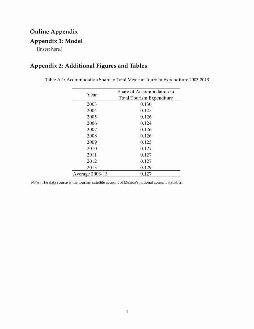
Online Appendix

Appendix 1: Model[Insert here.]

Appendix 2: Additional Figures and Tables

Table A.1: Acommodation Share in Total Mexican Tourism Expenditure 2003-2013

Year Share of Accommodation in Total Tourism Expenditure

2003 0.1302004 0.1252005 0.1262006 0.1242007 0.1262008 0.1262009 0.1252010 0.1272011 0.1272012 0.1272013 0.129

Average 2003-13 0.127Notes: The data source is the tourism satellite account of Mexico’s national account statistics.

1

Figure A.1: Tourist Arrivals in Mexico (in Millions)

0

2

4

6

8

10

12

1419

62

1964

1966

1968

1970

1972

1974

1976

1978

1980

1982

1984

1986

1988

1990

1992

1994

1996

1998

2000

2002

2004

2006

2008

Annual Number of International Tourists (Millions)

Notes: The data source is the Mexican Secretariat for Tourism (SECTUR). The depicted time series of arrivals refers to"interior tourists" and excludes so called "border tourists" that cross the border but do not move on to Mexico’s interior.For example in 2008, Mexico reported a total of 23 million international tourists of which 13.5 million were interiortourists (depicted) and 9.5 million were border tourists.

Table A.2: Wavelength Ranges Among the Top Four Beaches in Mexico

min max min max min max min max min max min maxPlaya del Carmen 72 125 67 110 79 120 119 175 69 142 41 93

Tulum 81 106 74 94 99 120 121 153 97 133 56 84

Cozumel 71 111 66 101 78 102 113 157 96 138 59 86

Cancun 81 111 72 101 74 102 38 149 15 125 7 71

Bandwidth 6Beaches Bandwidth 1 Bandwidth 2 Bandwidth 3 Bandwidth 4 Bandwidth 5

Notes: The table presents the wavelength ranges of the top four beaches in Mexico a identified by U.S. News. The datasource are LandSat satellite data from 1980s and 90s at a resolution of 30x30 meters.

2

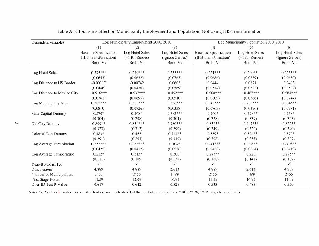
Table A.3: Tourism’s Effect on Municipality Employment and Population: Not Using IHS Transformation

Dependent variables:(1) (2) (3) (4) (5) (6)

Baseline Specification (IHS Transformation)

Log Hotel Sales (+1 for Zeroes)

Log Hotel Sales (Ignore Zeroes)

Baseline Specification (IHS Transformation)

Log Hotel Sales (+1 for Zeroes)

Log Hotel Sales (Ignore Zeroes)

Both IVs Both IVs Both IVs Both IVs Both IVs Both IVs

Log Hotel Sales 0.275*** 0.279*** 0.255*** 0.221*** 0.200** 0.225***(0.0643) (0.0632) (0.0763) (0.0686) (0.0859) (0.0680)

Log Distance to US Border -0.00217 -0.00742 0.0603 0.0444 0.0871 0.0403(0.0486) (0.0470) (0.0569) (0.0514) (0.0622) (0.0502)

Log Distance to Mexico City -0.516*** -0.537*** -0.452*** -0.568*** -0.487*** -0.584***(0.0761) (0.0695) (0.0510) (0.0809) (0.0566) (0.0744)

Log Municipality Area 0.282*** 0.308*** 0.256*** 0.343*** 0.289*** 0.364***(0.0810) (0.0726) (0.0338) (0.0863) (0.0376) (0.0781)

State Capital Dummy 0.570* 0.568* 0.783*** 0.540* 0.728** 0.538*(0.304) (0.298) (0.304) (0.328) (0.339) (0.323)

Old City Dummy 0.809** 0.834*** 0.980*** 0.836** 0.947*** 0.855**(0.323) (0.313) (0.290) (0.349) (0.320) (0.340)

Colonial Port Dummy 0.483* 0.463 0.714** 0.589* 0.824** 0.572*(0.291) (0.291) (0.310) (0.308) (0.355) (0.307)

Log Average Percipitation 0.253*** 0.263*** 0.104* 0.241*** 0.0968* 0.249***(0.0425) (0.0412) (0.0536) (0.0428) (0.0564) (0.0419)

Log Average Temperature 0.212* 0.213* 0.200 0.273** 0.220 0.275**(0.111) (0.109) (0.137) (0.108) (0.141) (0.107)

Year-By-Coast FX Observations 4,889 4,889 2,613 4,889 2,613 4,889Number of Municipalities 2455 2455 1489 2455 1489 2455First Stage F-Stat 11.59 12.09 16.95 11.59 16.95 12.09Over-ID Test P-Value 0.617 0.642 0.528 0.533 0.485 0.550

Log Municipality Employment 2000, 2010 Log Municipality Population 2000, 2010

Notes: See Section 3 for discussion. Standard errors are clustered at the level of municipalities. * 10%, ** 5%, *** 1% significance levels.

3

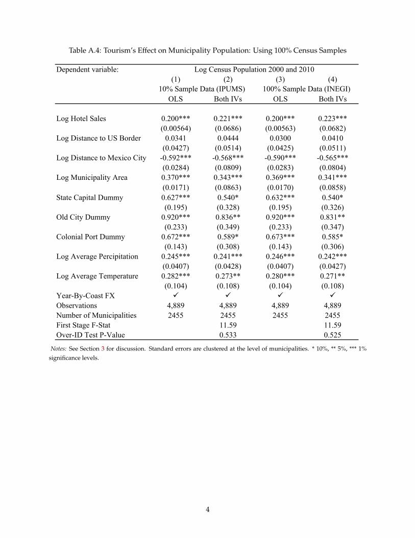
Table A.4: Tourism’s Effect on Municipality Population: Using 100% Census Samples

Dependent variable:(1) (2) (3) (4)

OLS Both IVs OLS Both IVs

Log Hotel Sales 0.200*** 0.221*** 0.200*** 0.223***(0.00564) (0.0686) (0.00563) (0.0682)

Log Distance to US Border 0.0341 0.0444 0.0300 0.0410(0.0427) (0.0514) (0.0425) (0.0511)

Log Distance to Mexico City -0.592*** -0.568*** -0.590*** -0.565***(0.0284) (0.0809) (0.0283) (0.0804)

Log Municipality Area 0.370*** 0.343*** 0.369*** 0.341***(0.0171) (0.0863) (0.0170) (0.0858)

State Capital Dummy 0.627*** 0.540* 0.632*** 0.540*(0.195) (0.328) (0.195) (0.326)

Old City Dummy 0.920*** 0.836** 0.920*** 0.831**(0.233) (0.349) (0.233) (0.347)

Colonial Port Dummy 0.672*** 0.589* 0.673*** 0.585*(0.143) (0.308) (0.143) (0.306)

Log Average Percipitation 0.245*** 0.241*** 0.246*** 0.242***(0.0407) (0.0428) (0.0407) (0.0427)

Log Average Temperature 0.282*** 0.273** 0.280*** 0.271**(0.104) (0.108) (0.104) (0.108)

Year-By-Coast FX Observations 4,889 4,889 4,889 4,889Number of Municipalities 2455 2455 2455 2455First Stage F-Stat 11.59 11.59Over-ID Test P-Value 0.533 0.525

Log Census Population 2000 and 2010

10% Sample Data (IPUMS) 100% Sample Data (INEGI)

Notes: See Section 3 for discussion. Standard errors are clustered at the level of municipalities. * 10%, ** 5%, *** 1%significance levels.

4