Total Factor Productivity and Relative Prices: the case of Italy

Giorgio Garau

University of Sassari – Department of Humanistic and Social Sciences

Stefano Deriu

University of Macerata – Department of Economics and Law

DRAFT

1. Introduction

Fontela in his seminal work (1989) set up the distributional rule of productivity gain in the Input–Output

context (Total Factor Productivity Surplus, TFPS). Garau (1996) proposed an extension to identify a

measure of surplus, called Purchasing Power Transfer (PPT). This measure is given by the productivity

gains and the market surplus generated by extra–profits conditions derived from rental position

detained by agents. Such a decomposition is very useful from our point of view since it would provide

information about the degree of non–competitiveness in different markets. In our paper, we compute

and explain Fontela’s TFPS comparing it with Garau’s PPT for Italy for the year 2009-2014.

2. Theoretical famework

During the 70s and the 80s most of the industrialised countries experienced a fall in productivity.

However, this phenomenon did not affect the USA that, especially in the 90s, has seen a growth in

productivity and a bigger economic growth, thanks to the development of ICT and to the rise of the

‘New Economy’. Fontela (2002) argues that this is a typical mesoeconomic effect, whose dimension

lies between the impact of structural changes in the technology of production (effects on efficiency)

and what has been observed at a macroeconomic level (effects on the growth). To better

understand these processes it is useful to refer to Baumol (1967) and to his model of unbalanced

growth. The model considers two sectors, one is increasingly more productive and the other is in a

situation of stagnation. In an economy characterised by perfect mobility of labour, the unbalance

determines a reduction of costs and prices in the first sector, especially if there is substitutability

between goods, and this could determine the disappearance of the sector whose productivity is not

growing. Sectors with a stagnant productivity often produce goods with an inelastic price (e.g. the

artistic activities), and therefore the surplus transfers end up subsidising these activities. If instead the

production of the two sectors is held in a fixed proportion, one would observe a progressive spill over

of labour towards the less productive sector. This hypothesis have been empirically tested in different

works (Baumol, Blackman and Wolf, 1985, Appelbaum and Schekatt, 1994). Another cause of this

differential evolution can be found in the structure of the market which characterises the different

sectors. Fontela, Lo Cascio e Pulido (2000) found that in general there is an inverse correlation

between prices and productivity, except for those sectors, such as agriculture, for which prices are

distorted by the intervention of the Government. In short, their analysis allows to state that one of the

principal causes of the unbalanced growth is the structure of the market, therefore the existence of

imperfect competition, where prices do not adjust according to technical changes. The relation

between technical changes, market structure and prices has been analysed by Anne Carter (1990)

in a model where, similarly to Baumol, it is considered an economic system composed by subsets of

sectors, innovative sectors and sectors where no change in technology is observed. Results clearly

show that the distribution of the innovation gains strongly depends on the structure of the market,

and determines both an increase in profits, in the case where the advantages go to the capital

holders, and a reduction of prices, in the case where the benefits go to the consumers under the

form of increased purchasing power. All the cited studies underline the necessity of understanding

what happens to prices and income when the effect of the innovation begins. For instance when at

a certain time a productivity gain is observed, it is still not possible to say whether it would be

preferable to obtain a long run price reduction, an income rise of different factors, or a combination

of the possible effects. In this case, it is clear that an answer can be provided by using CGE models.

For instance, the FSD model (Fontela, Solari and Duval, 1971) that links the demand function and the

production function, cited in Fontela (2002) constitutes a sort of precursor. The cited contribution by

Baumol and Carter allow to better understand the mechanism of unbalanced growth which has

characterised the New Economy in the following way (Fontela, 2002). The 90s productivity growth in

the USA is certainly based on the introduction of ICT in most of the productive sectors. In fact, as one

would expect, in a situation of perfect competition, this should produce a reduction of prices of all

the goods that incorporate the new technology, and this process can be accelerated by the

intervention of the Government for the dismantlement of public monopolies (e.g.

telecommunications). At the same time, wages of specialised workers would rise, and possibly the

surplus would be partially absorbed by those sectors owning patents in the ICT. What happens now

to the demand will depend on the elasticity of consumption with respect to prices and income, and,

if the elasticity of goods and services with high technological content is high, one should see a chain

effect where a rise in demand stimulates innovation, prices fall and the demand rises again. This

dynamic, typical of the New Economy, will end up when the system is saturated of high tech goods,

and, in any case, in the final phase, only a high rate of innovation would allow the system to keep

growing. Because the growth mechanism here described is highly unbalanced, it is necessary to try

to govern it through public policies capable of avoiding social and financial global crisis (Fontela

2002). These last words of Fontela seem to predict the big economic/financial global crisis of 2008,

whose effects are still perceived nowadays. His analysis is truly precious to understand why currently,

a world that evolves at different speeds is still unable to firmly restart and leave stagnation behind. It

is important to study the effects of innovation to understand what the public sector can do to help

firms innovating and therefore to stimulate economic growth, as well as what could be done to avoid

that the benefits of innovation, when existing, are entirely allocated to private sector and enterprises

(Mazzucato 2014). This topic is linked to a correct design of cluster policies (those policies called smart

specialisation strategy at an European and regional level) and to subsidies to the firms. In general

when government resources are used, especially when its use can produce distortions, it would be

opportune to perform an ex ante impact evaluation of the interventions, in order to better define the

implementation and to report to the population costs and benefits of such policy. On this point,

clearly explained by Mazzucato (2014), Fontela’s contribution on the nature of surplus redistribution

generated by technological progress between firms/sectors composing the economic system is

extremely important. The Emilio Fontela lesson, who began studying these issues in the 80s applying

surplus distribution measures based on macroeconomic accounting systems (national states) or

microeconomic ones (enterprises), is fundamental to understand, today, the distribution dynamics

that trigger once the progress and innovation benefits appear. In his seminal paper (1989), the

principal finding was that “a growth process does not only imply a path of generation of TFP, it also

includes an internal transfer between industries of the gains of TFP”. Moreover, in Fontela (1993), he

states that “the rule of distribution will finally be dictated by the structure of the different markets ...

with perfect competition in all markets for products and primary factors, consumers will benefit

immediately following price decrease but in all cases of more or less imperfect competition, the

results will be less clear”. In his work, Fontela qualifies his results relating to Spain as a demonstration

of the appearance of an unbalanced growth path between manufacturing and services sectors

(Baumol and Wolff, 1984). It is now clear which is the fundamental contribution of Fontela in providing

valuable insights into the nature of productivity growth in order to design structural policies adeguate

to foster economic growth. The paper is then organized as follows. Section 3 contains illustration and

theoretical justification of the Fontela system of surplus distribution. In section 4 we propose a method

to calculate implicit price indexes, using input-output tables. Section 5 propose the Garau’s PPT

distributional rules. In Section 6 we propose the results of our research and finally, in the last section,

we show three possible ways of extend TFPS/PPT analysis in order to support the dissemination of

Fontela’s idea and to make its approach a more useful tool for economic analysis and policy

evaluation.

3. Fontela’s TFPS model

Fontela (1989) calls TFPS the differences between output and inputs, both measured at constant

prices. The idea is based on the Input-Output table deflection at current prices, in order to obtain an

"unbalanced" table at constant prices, ie a table in which the total row does not coincide with the

total column; the difference between general total row and and column provides the TFPS. In order

to obtain national accounting data at constant prices it is possible to adopt two different

methodologies (Garau 1996):

- using price indices;

- using quantity indices.

In the first case we start from a table with prices and quantities of the current year:

∑𝑃𝑖𝑗0𝑄𝑖𝑗𝑡 =∑𝑃𝑖𝑗𝑡𝑄𝑖𝑗𝑡𝑃𝑖𝑗𝑡/𝑃𝑖𝑗0

𝑗𝑗

In the second case we start from a table with prices and quantities of the base year:

∑𝑃𝑖𝑗0𝑄𝑖𝑗𝑡 =∑𝑃𝑖𝑗0𝑄𝑖𝑗0𝑄𝑖𝑗𝑡𝑄𝑖𝑗0

𝑗𝑗

Regardless of the used method used, having two Input-Output tables available at current and

constant prices, it is possible to calculate the difference between them:

∑𝑝𝑖𝑗𝑡 ∗ 𝑞𝑖𝑗𝑡𝑗

−∑𝑝𝑖𝑗0 ∗ 𝑞𝑖𝑗𝑡

𝑗

If this difference is positive, it means that the "j" sector sells its production at an higher price than the

price of the base year, withholding surplus productivity; on the contrary, the "j" sector sells at a lower

price, transferring productivity surplus to other sectors and to final consumers. From a productive

point of view we have:

∑𝑝𝑗𝑖𝑡 ∗ 𝑞𝑗𝑖𝑡𝑗

−∑𝑝𝑗𝑖0 ∗ 𝑞𝑗𝑖𝑡𝑗

In this case, positive value indicates that the "j" sector pays more the productive factors, transferring

productivity surplus to the other sectors and to the value added (capital and work); on the contrary,

the sector pays less for productive factors while retaining surplus productivity. Considering the

methodology proposed by Fontela for the calculation of TFPS, we can write:

𝑇𝐹𝑃𝑆𝑖𝑗 =∑𝑝𝑖𝑗0 ∗ 𝑞𝑖𝑗𝑡𝑗

−∑𝑝𝑗𝑖0 ∗ 𝑞𝑗𝑖𝑡

𝑗

(1)

This approach enjoys a relationship with Kendrik's productivity index:

𝑇𝐹𝑃𝑆𝑖𝑗 = (𝐾𝑇𝐹𝑃𝑖𝑡 − 1)(∑𝑃𝑗𝑖0 ∗ 𝑄𝑗𝑖𝑡)

𝑗

)

where

𝐾𝑇𝐹𝑃𝑖𝑡 =

∑ 𝑃𝑖𝑗0 ∗ 𝑄𝑖𝑗𝑡𝑗

∑ 𝑃𝑖𝑗𝑡 ∗ 𝑄𝑖𝑗𝑡𝑗

∑ 𝑃𝑗𝑖0 ∗ 𝑄𝑗𝑖𝑡𝑗

∑ 𝑃𝑗𝑖𝑡 ∗ 𝑄𝑗𝑖𝑡𝑗

which represents the change in the “j” sector purchasing power, divided by an index of the change

in purchasing power for the production factors remuneration used by the "j" sector.

Considering that in time “t” we have

∑𝑝𝑖𝑗𝑡 ∗ 𝑞𝑖𝑗𝑡 =∑𝑝𝑗𝑖𝑡 ∗ 𝑞𝑗𝑖𝑡𝑗𝑗

∑𝑝𝑖𝑗𝑡 ∗ 𝑞𝑖𝑗𝑡 −∑𝑝𝑗𝑖𝑡 ∗ 𝑞𝑗𝑖𝑡 = 0

𝑗𝑗

it is possible to rewrite formula n.1 as

𝑇𝐹𝑃𝑆𝑖𝑗 =∑𝑝𝑖𝑗0 ∗ 𝑞𝑖𝑗𝑡𝑗

−∑𝑝𝑗𝑖0 ∗ 𝑞𝑗𝑖𝑡𝑗

− [∑𝑝𝑖𝑗𝑡 ∗ 𝑞𝑖𝑗𝑡 −∑𝑝𝑗𝑖𝑡 ∗ 𝑞𝑗𝑖𝑡𝑗𝑗

]

𝑇𝐹𝑃𝑆𝑖𝑗 =∑𝑝𝑖𝑗0 ∗ 𝑞𝑖𝑗𝑡𝑗

−∑𝑝𝑗𝑖0 ∗ 𝑞𝑗𝑖𝑡𝑗

−∑𝑝𝑖𝑗𝑡 ∗ 𝑞𝑖𝑗𝑡 +∑𝑝𝑗𝑖𝑡 ∗ 𝑞𝑗𝑖𝑡𝑗𝑗

𝑇𝐹𝑃𝑆𝑖𝑗 = −∑𝑝𝑖𝑗𝑡 ∗ 𝑞𝑖𝑗𝑡 +∑𝑝𝑖𝑗0 ∗ 𝑞𝑖𝑗𝑡𝑗

+∑𝑝𝑗𝑖𝑡 ∗ 𝑞𝑗𝑖𝑡 −∑𝑝𝑗𝑖0 ∗ 𝑞𝑗𝑖𝑡𝑗𝑗𝑗

𝑇𝐹𝑃𝑆𝑖𝑗 = −∑𝑞𝑖𝑗𝑡 ∗ (𝑃𝑖𝑗𝑡 − 𝑃𝑖𝑗0)

𝑗

+∑𝑞𝑗𝑖𝑡 ∗ (𝑃𝑗𝑖𝑡 − 𝑃𝑗𝑖0) (2)

𝑗

which represents how the productivity surplus is redistributed in the economic system, and this

depends on changes in output and inputs prices. The model can be transferred to an input-output

context:

𝑋 𝑒 �̅� : intermediate flows matrix at current and constant prices

𝑇 𝑒 �̅�: taxes minus products contributions vector at current and constant prices

𝑉𝐴 𝑒 𝑉𝐴̅̅ ̅̅ : value added at current and constant prices

𝑀 𝑒 �̅�: import vector at current and constant prices

𝐶 𝑒 𝐶̅: consumption matrix at current and constant prices

𝐼 𝑒 𝐼:̅ investments matrix at current and constant prices

𝐸 𝑒 �̅�: export vector at current and constant prices

Then we have

𝑇𝐹𝑃𝑆 = (𝑆𝑙

′ + 𝑠𝑇 + 𝑠𝑉𝐴 + 𝑠𝑀) − (𝑆𝑙 + 𝑠𝐶 + 𝑠𝐼 + 𝑠𝐸) (3)

where

𝑆[𝑠𝑖𝑗] = 𝑋 − �̅�

[𝑠𝑇] = 𝑇 − �̅� [𝑠𝑉𝐴] = 𝑉𝐴 − 𝑉𝐴̅̅ ̅̅ [𝑠𝑀] = 𝑀 − �̅� [𝑠𝐶] = 𝐶 − 𝐶̅ [𝑠𝐼] = 𝐼 − 𝐼 ̅[𝑠𝐸] = 𝐸 − �̅�

Results: - 𝑆[𝑠𝑖𝑗] > 0: "j" sector transfers surplus to the "i" sector by intermediate inputs

- 𝑠𝑇𝑖 > 0: "j" sector transfers surplus to the State

- 𝑠𝑉𝐴𝑖 > 0: "j" sector transfers surplus to the primary inputs (Capital and Work)

- 𝑠𝑀𝑖 > 0 "j" sector transfers surplus to the rest of the world

- 𝑠𝐶𝑖 < 0: "j" sector transfers surplus to the consumers

- 𝑠𝐼𝑖 < 0: "j" sector transfers surplus to the investors

- 𝑠𝐸𝑖 < 0 "j" sector transfers surplus to the rest of the world

4. Implicit price indexes and TFPS transfers

The idea behind this work is the construction of sector price indexes to be used for the deflation of

the Italian Input-Output table referred to the year 2014. In particular, the central idea is the use of

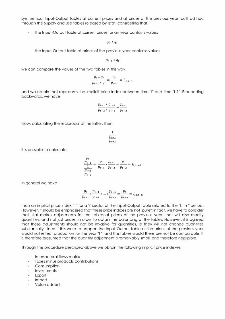
symmetrical Input-Output tables at current prices and at prices of the previous year, built ad hoc

through the Supply and Use tables released by Istat. considering that:

- the Input-Output table at current prices for an year contains values

𝑝𝑡 ∗ 𝑞𝑡

- the Input-Output table at prices of the previous year contains values

𝑝𝑡−1 ∗ 𝑞𝑡

we can compare the values of the two tables in this way

𝑝𝑡 ∗ 𝑞𝑡𝑝𝑡−1 ∗ 𝑞𝑡

=𝑝𝑡𝑝𝑡−1

= 𝐼𝑖;𝑡,𝑡−1

and we obtain that represents the implicit price index between time "t" and time "t-1". Proceeding

backwards, we have

𝑝𝑡−1 ∗ 𝑞𝑡−1𝑝𝑡−2 ∗ 𝑞𝑡−1

=𝑝𝑡−1𝑝𝑡−2

Now, calculating the reciprocal of the latter, then

1𝑝𝑡−1𝑝𝑡−2

it is possibile to calculate

𝑝𝑡𝑝𝑡−11𝑝𝑡−1𝑝𝑡−2

= 𝑝𝑡𝑝𝑡−1

∗𝑝𝑡−1𝑝𝑡−2

=𝑝𝑡𝑝𝑡−2

= 𝐼𝑖;𝑡,𝑡−2

In general we have

𝑝𝑡𝑝𝑡−1

∗𝑝𝑡−1𝑝𝑡−𝑘

∗ … ∗𝑝𝑡−𝑘𝑝𝑡−𝑛

=𝑝𝑡𝑝𝑡−𝑛

= 𝐼𝑖;𝑡,𝑡−𝑛

than an implicit price index “I” for a "i" sector of the Input-Output table related to the "t, t-n" period.

However, it should be emphasized that these price indices are not "pure"; in fact, we have to consider

that Istat makes adjustments for the tables at prices of the previous year, that will also modify

quantities, and not just prices, in order to obtain the balancing of the tables. However, it is agreed

that these adjustments should not be invasive for quantities, ie they will not change quantities

substantially, since if this were to happen the Input-Output table at the prices of the previous year

would not reflect production for the year "t ", and the tables would therefore not be comparable. It

is therefore presumed that the quantity adjustment is remarkably small, and therefore negligible.

Through the procedure described above we obtain the following implicit price indexes:

- Intersectoral flows matrix

- Taxes minus products contributions

- Consumption

- Investments

- Export

- Import

- Value added

The price indices are then transformed into relative price indexes, comparing the price index with

respect to the reference weighted average. Given an “X” vector, we have:

𝐼 ̅ =𝐼𝑖;𝑡,𝑡−𝑛 ∗ 𝑋𝑖∑ 𝑋𝑖 𝑖

And the relative price index is given by

𝐼𝑖;𝑡,𝑡−𝑛𝑟𝑒𝑙 = 𝐼𝑖;𝑡,𝑡−𝑛 ∗ 𝐼 ̅

Through the relative price indexes, the Input-Output table for the year 2014 is deflated at 2009 prices,

and subsequently the TFPS are calculated using formula 3

5. Garau’s PPT model

In the model proposed by Fontela, the effect of its variation due to the behavior of the economic

system agents and markets, is not highlighted; in particular, the ability that some agents have to

change prices is reflected on the𝑇𝐹𝑃𝑆𝑖𝑗 . Garau (1996), propose a model based on the 𝑇𝐹𝑃𝑆𝑖𝑗

decomposition. The price is divided into two parts:

𝑝𝑖𝑗0 = 𝑝𝑖𝑗0

∗ + 𝑝𝑖𝑗0∗∗

- 𝑝𝑖𝑗0∗ it represents the market price that should be had if agents were not able to obtain extra

profits (price under competition);

- 𝑝𝑖𝑗0∗∗ represents the change in price compared to the one in competition due to the behavior of

economic agents, ie their ability to create extra profits (Martek Surplus)

Considering what has been said, the 𝑇𝐹𝑃𝑆𝑖𝑗 can therefore be decomposed as follows:

𝑇𝐹𝑃𝑆𝑖𝑗 = −∑𝑞𝑖𝑗𝑡 ∗ (𝑝𝑖𝑗𝑡 − 𝑝𝑖𝑗0∗ − 𝑝𝑖𝑗0

∗∗ )

𝑗

+∑𝑞𝑗𝑖𝑡 ∗ (𝑝𝑗𝑖𝑡 − 𝑝𝑗𝑖0∗ − 𝑝𝑗𝑖0

∗∗ )

𝑗

𝑇𝐹𝑃𝑆𝑖𝑗 = −∑𝑞𝑖𝑗𝑡 ∗ (𝑝𝑖𝑗𝑡 − 𝑝𝑖𝑗0∗ )

𝑗

+∑𝑞𝑖𝑗𝑡 ∗ 𝑝𝑖𝑗0∗∗

𝑗

+

𝑇𝐹𝑃𝑆𝑖𝑗 = +∑𝑞𝑗𝑖𝑡 ∗ (𝑝𝑗𝑖𝑡 − 𝑝𝑗𝑖0∗ )

𝑗

−∑𝑞𝑗𝑖𝑡 ∗ 𝑝𝑗𝑖0∗∗

𝑗

+

Optimal 𝑇𝐹𝑃𝑆𝑖𝑗 is defined as

𝑇𝐹𝑃𝑆𝑖𝑗∗ = −∑𝑞𝑖𝑗𝑡 ∗ (𝑝𝑖𝑗𝑡 − 𝑝𝑖𝑗0

∗ )

𝑗

+∑𝑞𝑗𝑖𝑡 ∗ (𝑝𝑗𝑖𝑡 − 𝑝𝑗𝑖0∗ )

𝑗

While 𝑀𝑆𝑖𝑗 is defined as

𝑀𝑆𝑖𝑗 =∑𝑞𝑖𝑗𝑡 ∗ 𝑝𝑖𝑗0∗∗

𝑗

−∑𝑞𝑗𝑖𝑡 ∗ 𝑝𝑗𝑖0∗∗

𝑗

Then the 𝑃𝑃𝑇𝑖𝑗 is given by

𝑃𝑃𝑇𝑖𝑗 = 𝑇𝐹𝑃𝑆𝑖𝑗 = 𝑜𝑝𝑡𝑖𝑚𝑎𝑙 𝑇𝐹𝑃𝑆𝑖𝑗

+𝑀𝑆𝑖𝑗

Considering the difference between terms of last equations, we observe that

- Optimal 𝑇𝐹𝑃𝑆𝑖𝑗 has a positive value if the second term is bigger than the first term; this means

that the "i" sector generates and distributes purchasing power attributable to an increase in

productivity;

- 𝑀𝑆𝑖𝑗 , on the contrary, has a negative value if the second term is bigger then the first term; This

means that a negative value corresponds to a redistribution of purchasing power.

We can estimate optimal 𝑇𝐹𝑃𝑆𝑖𝑗 using Törnqvist Index Price (Wolf, 1985 e 1989, Fontela, 1994) as a 𝑃𝑖𝑗

∗

proxy. The Törnqvist index price is calculated in the following way:

𝑇𝑖,𝑡−𝑛,𝑡 =∏(𝑝𝑖,𝑡𝑝𝑖,𝑡−𝑛

)

𝑤𝑖,𝑡−𝑛+𝑤𝑖,𝑡2

𝑖

As we can see, the Törnqvist price index is unique for the entire "i" row of the Input-Output table, ie

we consider that the price charged by a sector “i” to its products used as intermediate inputs is the

same for all the purchasing sectors “j”. For each sector "i" the relationship between prices is derived

by comparing the values contained in the intersectorial matrices of the two tables

𝑃2014 ∗ 𝑃2014𝑄2014 ∗ 𝑃2009

=𝑃2014𝑃2009

In the formula, 𝑤𝑖,𝑡, represents the value portion of the asset produced by the "j" sector on the value

of the aggregate in the period t:

𝑤𝑖,𝑡 =𝑃𝑖,𝑡 ∗ 𝑄𝑖,𝑡∑ 𝑃𝑖,𝑡 ∗ 𝑄𝑖,𝑡𝑖

And the same is for 𝑤𝑖,𝑡−𝑛. At this point, we deflate the Inpuit-Output table for the year 2014 with

Törnqvist price index, and we reapplied the TFPS calculation procedure, in order to obtein the

optimal 𝑇𝐹𝑃𝑆𝑖𝑗 . The 𝑀𝑆𝑖𝑗

is obteined as resiudal:

𝑀𝑆𝑖𝑗 = 𝑃𝑃𝑇𝑖𝑗 − 𝑜𝑝𝑡𝑖𝑚𝑎𝑙 𝑇𝐹𝑃𝑆𝑖𝑗

It is important to underline that the positivity or negativity of the sectoral 𝑃𝑃𝑇𝑖𝑗 depends on the sign

of the optimal 𝑇𝐹𝑃𝑆𝑖𝑗 and the 𝑀𝑆𝑖𝑗

; the possible combinations are:

PPTij > 0,

{

[−∑𝑞𝑖𝑗𝑡 ∗ (𝑝𝑖𝑗𝑡 − 𝑝𝑖𝑗0

∗ )

𝑗

+∑𝑞𝑗𝑖𝑡 ∗ (𝑝𝑗𝑖𝑡 − 𝑝𝑗𝑖0∗ )

𝑗

] > 0; [∑𝑞𝑖𝑗𝑡 ∗ 𝑝𝑖𝑗0∗∗

𝑗

−∑𝑞𝑗𝑖𝑡 ∗ 𝑝𝑗𝑖0∗∗

𝑗

] > 0

[−∑𝑞𝑖𝑗𝑡 ∗ (𝑝𝑖𝑗𝑡 − 𝑝𝑖𝑗0∗ )

𝑗

+∑𝑞𝑗𝑖𝑡 ∗ (𝑝𝑗𝑖𝑡 − 𝑝𝑗𝑖0∗ )

𝑗

] > 0; [∑𝑞𝑖𝑗𝑡 ∗ 𝑝𝑖𝑗0∗∗

𝑗

−∑𝑞𝑗𝑖𝑡 ∗ 𝑝𝑗𝑖0∗∗

𝑗

] < 0

[−∑𝑞𝑖𝑗𝑡 ∗ (𝑝𝑖𝑗𝑡 − 𝑝𝑖𝑗0∗ )

𝑗

+∑𝑞𝑗𝑖𝑡 ∗ (𝑝𝑗𝑖𝑡 − 𝑝𝑗𝑖0∗ )

𝑗

] < 0; [∑𝑞𝑖𝑗𝑡 ∗ 𝑝𝑖𝑗0∗∗

𝑗

−∑𝑞𝑗𝑖𝑡 ∗ 𝑝𝑗𝑖0∗∗

𝑗

] > 0

PPTij < 0,

{

[−∑𝑞𝑖𝑗𝑡 ∗ (𝑝𝑖𝑗𝑡 − 𝑝𝑖𝑗0

∗ )

𝑗

+∑𝑞𝑗𝑖𝑡 ∗ (𝑝𝑗𝑖𝑡 − 𝑝𝑗𝑖0∗ )

𝑗

] < 0; [∑𝑞𝑖𝑗𝑡 ∗ 𝑝𝑖𝑗0∗∗

𝑗

−∑𝑞𝑗𝑖𝑡 ∗ 𝑝𝑗𝑖0∗∗

𝑗

] < 0

[−∑𝑞𝑖𝑗𝑡 ∗ (𝑝𝑖𝑗𝑡 − 𝑝𝑖𝑗0∗ )

𝑗

+∑𝑞𝑗𝑖𝑡 ∗ (𝑝𝑗𝑖𝑡 − 𝑝𝑗𝑖0∗ )

𝑗

] > 0; [∑𝑞𝑖𝑗𝑡 ∗ 𝑝𝑖𝑗0∗∗

𝑗

−∑𝑞𝑗𝑖𝑡 ∗ 𝑝𝑗𝑖0∗∗

𝑗

] < 0

[−∑𝑞𝑖𝑗𝑡 ∗ (𝑝𝑖𝑗𝑡 − 𝑝𝑖𝑗0∗ )

𝑗

+∑𝑞𝑗𝑖𝑡 ∗ (𝑝𝑗𝑖𝑡 − 𝑝𝑗𝑖0∗ )

𝑗

] < 0; [∑𝑞𝑖𝑗𝑡 ∗ 𝑝𝑖𝑗0∗∗

𝑗

−∑𝑞𝑗𝑖𝑡 ∗ 𝑝𝑗𝑖0∗∗

𝑗

] > 0

6. Results

In the following tables we report the results about:

- Table 1: PPT distribution in Italy, 2009 – 2014

- Table 2: Optimal TFPS distribution in Italy, 2009 – 2014

- Table 3: MS distribution in Italy, 2009 – 2014

- TABLE 4: PPT > 0 decomposition

- TABLE 5: PPT < 0 decomposition

- TABLE 6: Price Indexes

The results show the performance of sectors in terms of PPT, optimal TFPS and MS. It is interesting to

carry out an analysis of the same from the point of view of the sectoral efficiency, considering in

particular the case of positive optimal TFPS results.

The best performance is showed by "Extractive activities" and "Manufacturing of other non-

metalliferous mineral processing products", with optimal TFPS equal respectively to 17,290 and 13,539

milions euros. These two sectors show also a positive MS, which means that for both sectors, PPT results

from the efficiency of the system (capacity of the system to create surplus of productivity) and from

the capacity of the agents to create additional surplus, using their Market power, by reducing sales

prices. However, from a redistributive point of view, we observe that 50% of MS is transferred to the

rest of the world through imports, while the remaining 50% is transferred to other sectors through an

increase in the intermediate inputs remuneration. Another efficient sector is "Supply of electricity, gas,

steam and air conditioning" with a value of optimal TFPS equal to 10,298 milions euros. However, part

of such surplus, about 54%, is retained in the form of extra profits, which means that agents are able,

through market distortions, to maintain higher prices, generating a negative MS. Of major

importance is the result of the sector "Land transport and transport by pipelines". In this case we have

an efficient sector, which creates surplus of productivity for 4.53 billion euros, but through the market

power agents arrive to retain, increasing their prices, more than the generated TFPS and finally we

observe a negative PPT.

In terms of optimal negative TFPS, we observe that "Construction" represents absolutely the worst

performance, with a value of-26,584 milions euros. In particular, we found that the greater share of

surplus is retained by investments, as well as by intermediate inputs. On the import side the sector

transfers surplus to the rest of the world. Looking now at the MS circuit we observe a small surplus

generation of 5.058 billion euros, negligible compared to the loss of productivity. Moreover, this quota

is transferred mostly to public consumption. Another non-performing sector is "Provision of financial

services (excluding insurance and pension funds)" charactherized by a strongly negative optimum

TFPS, -24,865 milions euros. It is to be noted that this sector retains surplus from other production sectors

through intermediate inputs, but also from added value, imports and consumers (households). The

MS registers a value of 7.605 billion euros, too low to compensate the loss of productivity surplus, and

then we register a negative PPT. Lastly, negative optimal TFPS is a charactheristics of the “Food,

beverage and tobacco industries", with a value of-6.609 billion euros. In this case, the sector retains

surplus from other sectors through intermediate inputs prices, but also from added value, imports and

consumers (households). Finally this sector registers a negative MS, generating extra profits for

economic agents for -200 million euros.

Lastly, the following sectors deserve special attention:

- "Health services activities". This sector is not efficient, even if the inefficiency is close to zero, (-853

million euros). However, the sector redistribute surplus through market power, reducing prices versus

intermediate inputs, VA and the Rest of the world and augmenting prices versus Households.

-"Land transport and transport by pipelines" is an efficient sector (optimal TFPS of 4.53 billion euros)

but registers a MS of-4.708 billion euros, thus producing a negative PPT. It means that the surplus of

productivity generated by the efficiency of the market is retained in the form of extra profits.

-"Manufacture of coke and petroleum refining products" is the sector with the worst performance in

MS, with a value of-13,733 milions euros. The sector is not efficient (optimal optimum TFPS equal to -

350 million euros, close to zero) but the strong market power allows it to increase intermediate inputs

prices and in fact this sector retains surplus from other sectors for about 98%.

7. Further Topics Under Inspection

Fontela closes his seminal paper (Fontela, 1989) describing an alternative model of growth where

the long–term trend of increasing relatives prices in services changes in order to allow a process of

TFPS transfers. Nowadays the role of the service sector belong to renewable energies, green

chemistry or “internet of things” (Rifkin, 2014), as these are sectors where a big concentration of

research and innovation will probably produce TFP gains able to push the economy towards a new

deal. In this Section, conceived as a road map for further inspection of area where TFPS analysis

could be improved and become a useful tool for economic analysis and policy evaluation, we try

to stress how the Fontela contribution today represents an inheritance rich of further suggestions.

7.1 Prices

Prices are fundamental, as seen in Sections 3, 4 and 5, in order to obtain coherent measures of TFPS

and PPT. Moreover, in Garau (1997) and in Antille and Fontela (2003) a system of international prices

is conceived to give an insight to the spatial distribution of productivity gains.The first uses import and

export prices produced by the World Bank and his principal findings concern the possibility to design

different mechanisms of effect transmission from the national to the inter–country dimension,

depending on the national sectoral market power that is generally not strong enough to dominate

there distribution mechanism at the international level. This subject is really interesting in the European

federal context, in order to assess regional growth, understanding how some regions contribute to

other region’s growth. Antille and Fontela (2003) conceive a more detailed system of TFPS transfers,

distinguishing among domestic and imported input flows. Their evidence supports the Kaldor’sidea

(1976) that the evolution of the term of trade has to do with market structure and the example

proposed, of Swiss industries with high level of innovation, able to appropriate their innovation gains

by exporting at high prices in well differentiated markets, fits well with the Garau’s development of

Fontela idea.

7.2 Accounting System

The recent book of T. Piketty (2014), that rediscovers and provides new arguments for the Kuznets

Curve (1955), bringsback the focus of the economic discussion on the distribution of the surplus

between capital and labour, providing also empirical evidence of the long term with regards to

factors affecting it. Among convergence factors (i.e. reduction of inequalities, the most relevant is

the innovation and knowledge diffusion resulting from human capital investments as it allows an

increase in productivity and a positive effect one conomic growth. Clearly, the first divergence factor

is the absence of such investments but also the imbalance derived from wealth accumulation and

concentration processes. When the annual ROE is greater than the growth rate, the assets inherited

from the past grow faster than the production process; a minimum amount of capital income savings

is needed to allow capital growth increase faster than the overall economic growth. The labour–

capital conflict, ending up giving advantage to the capital side imposes to understand upstream

mechanisms producing such results. Difference between PPT and TFPS could be interpreted as inertia

in the adjustment mechanisms or, equivalently, as a distance from perfect competition and related

automatic adjustment mechanisms. In this view we find that an interesting research topic could be

the use of business registers of Job Centre (covering all dependent labour market movements, i.e.

entry and exit in labour market) and Academic Institutions (graduates archives) to build labour

market scenarios and to model how human capital policies (but also R&D policies) can determine

sectoral growth and contribute to define productivity growth pattern. Input–Output accounting

maintains its focus on production (where productivity gains are generated) and it is therefore

inadequate to capture the complexity of the interrelations between production and consumption.

Conversely, SAM accounting allows it. When the observed deviation from the optimal distributional

result depends on the asymmetric speeds of adjustment of prices under the hypothesis that a rapid

(low)adjustment of a specific price, means less (greater) dynamic rental positions for consumer,

workers or enterprises emerge. Some possible and useful results of TFPS/PPT analysis conducted in this

new accounting context concern the link among the generation of productivity gains in the

production area with other areas, likes that of social security, where arrive a huge amount of

resources produced by technical progress and/or augmented by market power. In this same

research line, implementation of accounting systems specifically integrated in the context of

national accounts, is to be considered the analysis contained in Lo Cascio, Carbonaro, Guidi (1998),

in which the authors use the satellite account of Transportation for structural analysis, in order to

understand how this sector will affect the profitability of the economic system. The main results of the

adoption of the TFPS transfer approach shows a strong absorption of TFPS from other branches,

accounting for 7% of GDP. Contributions come from the agricultural sector and the manufacturing

and at the level of primary factors is essential the contribution of labour, resulting in a clear loss of

welfare.

7.3 A modelling context

We need to have models useful for monitoring policies, able to estimate the possible long–term

behaviour of some fundamental macroeconomic variables when structural policies are

implemented. In that view we propose to go in depth in the modelling version constituted by CGE

models. The analysis of productivity distribution and the modelling of regional technical change

could be integrated in a CGE model in which the technology will be the most important variable in

explaining relationship on the supply side. Such a model will be able to capture the short and long

run effects (together with the transitional pathway) of an increase inproductivity and then forecasting

the productivity gains transfers among economic agents. Such model could be very helpful for the

policy maker when the aim is both to push on the productivity and the final destination to the primary

factors of the corresponding welfare gains. For example, if the regional government would invest in

R&D, the analysis of TFP surplus can suggest us which sector would be able to generate the highest

TFP and the surplus available for the distribution to the other agents. The picture of inter–industry

diffusion and distribution of the welfare gains of innovations provided by this model might be used to

manage the process of prices adjustment when the industrial policy takes the form of selective

subsidies. In fact, they can be oriented towards correction of imperfections in the market mechanism

or in favour of sectors that exhibit high rate of innovation in order to transfer massive welfare gains to

the rest of the economy. The standard CGE modelling approach, based on neoclassical assumptions

such as perfectly competitive markets and constant return to scale, leads to results on key

macroeconomic variables consistent with price competition. Conversely, in our analysis we are

interested in the study of the effects that a rise in an economic system when in a specific sector there

is evidence of imperfect competition. Usually, CGE models with imperfect competition are based on

the theory of product varieties that, in turn, is derived from the theory of industrial organisation all

owing the economies of scale instead of constant return to scale. These models are used, between

others applications, in order to assess the impact of the European unification in reducing inequalities,

labour market imperfections and as a modelling tool, to endogenise innovation and technical

progress that allows firms to determine their price mark–up endogenously and, in this way, to affect

consumers utility. The comparison between the long term simulation produced by the two models

(standard and with imperfect competition) may be a good instrument to design public policies in

order to support the process of diffusion of innovation, to choose which sectors need further

liberalization and finally to design a tax system that allows the community to take control of at least

part of the benefits of innovation, so that it can then support also in the future.

Sectors:

1

-

Plant and animal production, hunting and related services

2

-

Forestry and forest areas use

3

-

Fishing and aquaculture

4

-

Mining and quarry

5

-

Food, beverage and tobacco industries

6

-

Textile industries, packaging of clothing articles and leather goods

7

-

Wood industry and wood/cork products, except furniture; articles of straw and plaiting materials

8

-

Paper and paper products

9

-

Printing and reproduction on recorded media

10

-

Coke and products deriving from oil refining

11

-

Chemical products

12

-

Basic pharmaceutical products and pharmaceutical preparations

13

-

Rubber and plastic articles

14

-

Other products from the processing of non-metallic minerals

15

-

Metallurgical activities

16

-

Metal products, except machinery and equipment

17

-

Computers, electronics and optics products

18

-

Electrical equipment

19

-

Machinery and equipment

20

-

Motor vehicles, trailers and semi-trailers

21

-

Other means of transport

22

-

Furniture and other manufacturing industries

23

-

Repair and installation of machines and equipment

24

-

Supply of electricity, gas, steam and air conditioning

25

-

Collection, treatment and supply of water

26

-

Management of sewage networks; waste collection, treatment and disposal activities; material recovery; rehabilitation activities and other waste management services

27

-

Constructions

28

-

Trade and repair of cars and motorcycles

29

-

Trade to the ingrosso, excluded cars and of motorcycles

30

-

Trade to the detail, excluded cars and of motorcycles

31

-

Land transport and transport via pipelines

32

-

Maritime and water transport

33

-

Airplane transport

34

-

Warehousing and transport support activities

35

-

Postal services and courier activities

36

-

Accommodation services; catering service activities

37

-

Publishing activities

38

-

Cinematographic production, video and television programs, music and sound recordings; programming and transmission activi ties

39

-

Telecommunications

40

-

Computer programming, consultancy and related activities; information services activities

41

-

Provision of financial services (excluding insurance and pension funds)

42

-

Insurance, reinsurance and pension funds, excluding compulsory social insurance

43

-

Auxiliary activities of financial services and insurance activities

44

-

Real estate activities

45

-

Legal activities and accounting; activities of central offices; management consulting

46

-

Activities of architectural and engineering studies; testing and technical analysis

47

-

Scientific research and development

48

-

Advertising and market research

49

-

Other professional, scientific and technical activities; veterinary services

50

-

Rental and leasing activities

51

-

Research, selection, supply of personnel

52

-

Service activities of travel agencies, tour operators and booking services and related activities

53

-

Investigation and supervision services; service activities for buildings and landscapes; administrative and support activities for office functions and other business support services

54

-

Public administration and defense; compulsory social insurance

55

-

Instruction

56

-

Activities of health services

57

-

Social care

58

-

Creative, artistic and entertainment activities; activities of libraries, archives, museums and other cultural activities; activities concerning betting and casinos

59

-

Sports and entertainment activities

60

-

Activities of membership organizations

61

-

Repair of computers and goods for personal and household use

62

-

Other personal service activities

63

-

Activities of families and cohabitations as employers for domestic staff; production of undifferentiated goods and services for own use by households and cohabitants

Table 1: PPT Distribution in Italy, 2009 – 2014; values in millions of Euros

Intersectoral Tax Value added Import Household consumptions ISP consumptions PA consumptions Investiments Valuables Stocks Export Total

1 -160,30 30,11 1.239,11 799,27 494,21 -2,75 -1,64 7,92 0,12 729,15 461,53 219,65

2 22,79 -15,67 77,44 63,44 125,51 0,00 -3,03 0,00 0,00 1,42 5,99 18,11

3 -141,57 14,46 262,82 59,93 513,94 0,00 0,00 -3,62 -0,01 2,27 32,28 -349,23

4 19.234,49 30,67 -497,87 18.840,87 956,20 0,40 -2,90 -112,58 -0,02 -2.796,37 60,14 39.503,30

5 -1.519,56 140,70 -3.013,72 -1.739,30 3.478,38 0,77 -16,04 -80,07 -0,04 933,90 -3.839,61 -6.609,17

6 -96,96 105,24 -2.641,65 -122,95 3.611,66 -0,26 7,26 45,46 5,06 643,84 -4.454,28 -2.615,06

7 104,47 9,57 788,34 319,84 679,91 -8,39 15,76 178,65 32,60 -40,14 -39,50 403,31

8 189,62 22,27 -527,13 323,84 23,95 -0,03 -1,63 -16,72 0,26 144,79 -518,98 376,96

9 -883,02 -9,31 -590,02 241,19 150,67 -0,02 -0,95 18,31 1,52 29,77 156,21 -1.596,67

10 -6.554,74 57,27 2.734,18 3.055,19 6.448,64 0,00 6,57 49,86 1,04 1.898,23 4.970,50 -14.082,94

11 1.213,72 323,15 -1.521,68 2.011,28 699,92 5,00 12,95 452,42 0,24 876,85 -719,14 698,22

12 2.279,43 5,97 -1.194,60 -2.538,27 -940,41 1,13 341,14 1,98 -0,34 422,70 -4.694,26 3.420,61

13 -2.611,13 87,81 -1.336,43 -737,47 1.212,27 -0,37 -1,66 -75,43 9,90 275,13 -386,98 -5.630,06

14 8.232,56 70,59 163,03 8.363,32 1.665,35 -0,14 5,70 90,45 5,83 -1.113,20 -607,91 16.783,42

15 -452,08 -153,02 -2.697,34 6.042,00 452,36 0,22 2,68 125,78 93,85 838,53 3.586,39 -2.360,24

16 -2.400,30 42,08 15,62 -566,67 287,24 -0,12 6,48 2.066,62 16,97 449,00 -1.751,68 -3.983,78

17 2.526,80 9,97 1.278,13 408,95 -738,70 1,36 6,66 577,81 14,69 122,55 188,06 4.051,42

18 143,21 12,31 585,93 -1.218,40 447,56 0,40 -1,21 480,86 2,59 669,77 -1.497,12 -579,80

19 3.605,67 79,13 -2.587,33 -2.337,08 -111,14 -0,84 -4,65 1.209,49 5,77 1.253,75 -8.524,75 4.932,74

20 2.897,12 -23,18 -452,95 759,15 1.712,13 -1,07 -3,54 2.145,70 0,06 1.034,62 -4.885,40 3.177,63

21 432,15 -57,27 -187,48 1.357,62 627,18 1,56 -0,13 3.089,86 1,06 -742,75 -1.355,77 -75,97

22 -43,55 8,58 930,54 -1.176,76 1.749,16 -0,69 -0,05 378,86 410,50 276,60 -2.009,74 -1.085,84

23 -53,22 -3,79 698,17 -308,76 -67,66 -0,09 -1,93 1.175,09 -0,43 -353,94 -531,81 113,17

24 2.730,88 -966,60 -74,68 1.501,88 -1.645,69 -0,09 -12,70 166,99 1,32 -17,57 -93,09 4.792,31

25 -168,41 153,19 275,53 62,92 562,61 5,06 -9,02 -8,63 0,00 0,42 16,63 -243,83

26 2.580,77 129,45 2.365,40 1.067,09 187,42 1,49 -6,11 17,45 0,52 12,49 296,23 5.633,21

27 -11.084,01 349,14 13.823,83 130,90 131,97 0,22 -2.888,44 27.569,32 1,33 -8,23 -59,75 -21.526,58

28 -1.486,03 6,21 732,05 336,84 823,02 -0,04 3,67 1.682,39 0,46 12,25 248,18 -3.180,86

29 -5.237,90 56,87 -4.408,74 -2.583,48 1.488,04 0,91 -211,11 121,14 17,53 90,09 -3.229,54 -10.450,32

30 700,55 138,98 -3.632,38 -1.469,95 -2.079,99 -3,21 -247,04 23,47 0,98 -2,67 -2.358,00 403,65

31 -1.081,95 951,65 3.885,10 223,01 3.377,00 -0,10 566,94 100,16 -0,92 -38,61 152,04 -178,70

32 -475,07 46,70 382,67 94,90 539,94 0,89 37,89 17,74 0,04 -0,09 492,64 -1.039,87

33 799,83 -2,60 1.175,83 -182,54 -104,27 -0,07 -110,29 14,56 0,03 -0,09 -456,73 2.447,38

34 -589,61 140,85 687,28 -283,58 358,10 -0,28 97,55 -146,12 -0,58 -13,92 -72,05 -267,75

35 -304,18 46,58 369,01 -260,41 588,14 -0,06 20,34 15,00 0,53 1,32 -429,51 -344,76

36 2.185,01 242,46 -1.799,03 -148,61 -2.390,65 -91,28 -40,70 9,40 0,57 -2,20 -14,06 3.008,76

37 -746,52 -6,29 1.409,06 2,64 981,44 0,57 0,20 1.137,43 -0,43 41,20 311,39 -1.812,92

38 243,71 -5,32 1.110,11 99,07 358,64 -0,46 -0,17 250,75 0,14 -17,09 108,58 747,18

39 -4.384,57 -2,38 -3.989,72 635,93 1.619,55 1,79 11,28 517,90 1,62 -256,36 -426,39 -9.210,14

40 3.094,65 91,61 -1.196,21 -301,01 519,85 -3,94 -150,94 -4.812,42 1,54 35,90 -982,68 7.081,73

41 -10.066,30 -32,63 -10.284,00 -1.196,89 -3.720,59 -0,64 0,65 -103,55 0,00 3,08 -498,69 -17.260,08

42 1.636,15 54,01 2.466,39 562,01 1.351,77 -0,04 -0,10 -24,80 0,00 0,19 296,14 3.095,41

43 3.356,63 182,67 3.945,08 -591,74 -155,57 -0,02 -2,59 49,20 0,00 0,69 -247,15 7.248,09

44 -4.601,52 39,85 -1.568,20 272,94 -5.340,04 5,00 19,68 4.286,19 0,00 0,37 446,96 -5.275,09

45 -1.772,66 57,81 2.497,09 -744,64 126,13 3,51 -15,78 929,13 0,01 -44,47 -328,90 -632,03

46 -904,12 19,41 1.069,09 -302,53 66,14 -1,15 -70,93 254,25 0,01 -105,09 120,45 -381,83

47 339,30 66,31 -813,17 154,09 14,93 3,36 26,66 -353,45 0,00 -8,27 -786,86 850,16

48 -640,22 5,67 -978,48 254,82 46,31 -0,80 -5,31 -1,49 0,10 110,00 -5,53 -1.501,49

49 -853,27 19,52 199,67 126,68 386,31 -2,95 -122,61 -64,45 0,54 59,67 148,10 -912,01

50 -1.063,33 -1,15 -1.283,91 403,73 -9,94 -0,11 -0,09 -19,33 -0,38 4,03 -54,91 -1.863,91

51 -1.256,64 12,59 -966,72 206,78 -77,75 0,00 -12,37 -8,65 0,00 3,37 160,40 -2.068,99

52 -381,13 6,86 -174,68 345,96 433,94 -0,02 45,51 -18,59 -0,50 -1,87 337,00 -998,45

53 1.047,36 130,06 2.667,02 666,75 158,36 -0,98 -169,88 -21,55 0,00 131,14 782,56 3.631,54

54 -2.495,88 768,54 87,86 12,12 164,52 0,10 3.676,85 -28,69 0,00 3,42 1,06 -5.444,62

55 -82,34 109,57 -6.364,13 -61,99 836,28 12,70 -7.424,55 -19,01 0,01 1,20 -20,67 215,15

56 2.768,91 708,78 -2.039,04 -204,22 1.101,52 -89,85 -3.832,47 -30,26 15,55 13,14 -234,07 4.290,87

57 854,70 98,01 -22,37 1,52 -97,06 19,94 -387,99 1,26 0,02 -0,14 1,55 1.394,29

58 836,30 216,66 1.224,12 276,15 1.231,13 -13,14 68,46 33,62 27,46 -4,15 -124,02 1.333,86

59 -923,72 92,16 -190,94 1,04 774,02 13,74 46,17 19,90 -0,02 -13,24 -63,95 -1.798,09

60 257,11 12,87 241,31 -4,58 154,20 30,89 -104,94 5,18 0,00 0,51 5,96 414,92

61 -24,01 1,99 113,47 -13,58 196,47 0,00 1,29 10,33 1,25 -28,41 -64,47 -38,59

62 1.225,91 63,69 531,91 7,56 -440,05 -2,67 18,75 -32,51 0,02 86,68 -11,12 2.209,98

63 0,00 0,00 -1.374,85 0,00 -1.536,32 0,00 0,00 0,00 0,00 0,00 0,00 161,47

Total 0,00 4.791,37 -8.377,25 30.997,81 24.458,15 -115,64 -10.818,41 43.345,96 669,99 5.605,15 -32.992,08 -2.741,18

Table 2: Optimal TFPS distribution in Italy, 2009 – 2014; values in millions of Euros

Intersectoral Tax Value added Import Household consumptions ISP consumptions PA consumptions Investiments Valuables Stocks Export Total

1 -110,15 -47,90 809,12 735,00 1.373,36 -0,43 0,24 -6,76 -0,05 721,22 162,75 -864,26

2 115,42 7,89 95,39 61,19 104,20 0,00 -71,10 0,00 0,00 2,96 4,25 239,57

3 -85,37 6,04 374,12 -27,24 381,75 0,00 0,00 -0,05 -0,01 0,58 7,66 -122,37

4 8.523,52 -9,93 -312,57 8.723,00 370,70 0,38 -3,07 -114,37 -0,05 -511,32 -108,00 17.289,75

5 -4.785,72 -190,07 -785,11 -1.711,11 2.108,44 0,58 -10,14 -86,72 -1,44 1.151,67 -4.225,56 -6.408,84

6 -2.416,35 82,52 -858,61 -557,59 5.073,50 -0,46 10,69 10,21 1,04 616,08 -5.932,94 -3.528,15

7 -20,82 -33,22 768,91 360,14 627,39 -8,93 15,90 207,57 22,28 1,18 -97,36 306,97

8 515,59 97,13 -163,75 385,87 9,36 -0,02 -0,83 -11,72 -0,03 149,05 -258,17 947,20

9 -770,80 1,06 59,05 191,45 94,05 -0,03 -1,01 14,44 0,88 49,21 99,92 -776,70

10 7.009,61 94,61 2.892,25 2.513,65 6.633,54 0,03 7,88 64,91 1,05 2.255,89 3.896,78 -349,95

11 -247,99 -31,75 -367,41 1.772,91 734,13 4,81 25,03 473,08 -0,55 1.000,42 -1.845,05 733,90

12 2.304,33 -17,85 -311,08 -1.462,60 -757,97 0,48 785,90 -38,80 -1,63 415,37 -5.336,89 5.446,35

13 -2.378,22 -68,64 -1.083,50 -4,60 1.228,19 -0,42 -0,95 -67,48 6,25 293,03 -658,62 -4.334,95

14 6.051,96 10,69 1.034,30 6.162,74 1.443,57 -0,19 6,22 68,67 4,54 -1.058,52 -798,05 13.593,45

15 -1.706,86 -32,30 495,05 4.867,25 363,63 0,19 1,95 124,79 56,60 852,35 3.121,89 -898,26

16 -2.890,65 -105,33 -679,20 -378,55 200,57 -0,27 0,61 1.897,14 9,30 460,67 -2.143,27 -4.478,48

17 3.165,33 -15,97 37,50 5.119,98 715,26 0,77 9,33 950,95 8,37 127,36 -123,46 6.618,26

18 105,07 -1,05 582,25 -211,91 484,01 0,21 -0,47 446,36 1,33 607,26 -1.706,04 641,69

19 -708,15 -232,31 -4.566,37 -1.238,05 -140,29 -1,53 -3,58 843,49 2,85 1.082,55 -9.552,61 1.024,24

20 674,69 -159,34 -623,58 2.499,35 982,60 -2,49 -1,61 2.569,21 0,01 989,16 -5.295,08 3.149,31

21 -316,99 -137,09 -782,98 1.117,57 513,53 1,30 1,43 2.952,29 0,37 -1.302,48 -1.809,05 -476,88

22 -1.117,45 -42,62 -241,82 -511,21 1.556,14 -0,76 1,20 419,87 207,93 155,80 -2.324,26 -1.929,01

23 -439,05 -69,15 45,95 -90,74 -28,53 -0,10 -1,47 1.171,70 -0,92 -192,15 -488,63 -1.012,89

24 7.005,65 1.454,15 961,98 1.933,18 946,27 -0,06 8,25 101,84 -3,81 -15,38 19,82 10.298,02

25 -39,51 -29,74 -66,84 62,92 300,43 4,23 11,18 19,61 0,00 0,96 14,55 -424,13

26 3.941,46 48,00 881,85 1.002,27 -126,14 1,28 14,28 33,60 0,50 23,20 264,94 5.661,93

27 -13.053,96 227,41 10.891,61 73,61 -385,47 0,24 -163,71 25.334,87 -0,46 -20,88 -41,71 -26.584,22

28 -1.054,12 -9,74 1.075,94 352,47 973,64 -0,04 2,93 806,56 -0,73 9,57 211,99 -1.639,36

29 -2.465,15 -196,09 -1.541,16 -2.930,85 -1.025,25 0,74 -193,75 -817,33 -56,96 78,76 -4.036,56 -1.082,89

30 847,26 -270,44 -3.392,85 -1.228,90 -3.837,60 -6,82 9,84 -90,32 -64,52 -88,21 -2.858,81 2.891,51

31 2.646,46 -437,16 4.161,32 533,36 1.151,87 -0,04 556,73 123,39 5,28 -29,22 566,18 4.529,79

32 -418,02 -207,95 138,20 123,76 234,79 3,56 43,15 -30,16 -0,80 -0,17 745,80 -1.360,17

33 2.605,14 -48,52 1.727,58 -110,93 -566,82 -0,07 -110,14 12,84 0,03 -0,11 -354,30 5.191,85

34 1.261,95 14,88 -339,90 90,27 -409,04 -0,12 329,55 -118,37 -0,11 -11,74 -148,49 1.385,51

35 -104,67 81,24 455,86 -301,67 555,88 -0,06 19,04 15,21 0,55 1,34 -403,79 -57,39

36 2.311,38 -238,95 -773,92 -218,87 -3.915,73 -153,20 -6,49 9,98 -0,14 -1,06 -18,33 5.164,58

37 -180,11 -11,38 959,71 119,50 1.072,63 0,78 0,45 57,72 -0,59 46,52 180,83 -470,62

38 657,40 -32,85 1.250,16 107,48 150,65 -0,64 -0,01 252,19 0,04 -25,43 55,14 1.550,25

39 -3.388,00 -167,19 775,02 482,22 405,07 0,68 9,08 254,22 1,21 -301,67 -739,69 -1.926,86

40 3.524,81 231,87 -1.660,14 -92,46 171,84 -4,03 -114,69 -3.820,72 1,44 40,28 -1.190,14 6.920,10

41 -13.788,37 -307,97 -7.960,06 -1.277,18 2.284,88 -0,77 -0,47 -107,93 0,00 0,73 -644,89 -24.865,13

42 371,46 294,86 -87,34 830,70 3.152,70 0,00 0,52 -0,25 0,00 0,04 272,97 -2.016,29

43 4.643,91 61,79 2.339,38 -102,38 -220,42 -0,01 -0,65 62,54 0,00 0,53 -264,86 7.365,56

44 -864,03 188,50 -1.065,05 304,05 -2.989,03 4,91 92,05 4.393,92 0,00 0,07 371,40 -3.309,86

45 243,62 -121,16 629,03 -698,12 -127,54 -18,40 3,92 822,11 -0,02 -42,65 -280,71 -303,33

46 -41,25 -40,66 890,92 -378,09 66,66 -1,14 -80,67 219,20 -0,01 -119,61 142,95 203,55

47 86,77 -56,63 -820,42 170,40 18,95 0,85 46,49 -161,11 0,00 -11,06 -844,63 330,63

48 -684,23 -27,44 -172,39 125,84 37,79 -1,22 -7,12 -6,19 0,10 -260,56 -35,81 -485,21

49 -369,65 -39,26 -325,80 176,42 424,74 -2,98 -189,26 -86,36 0,35 78,84 255,79 -1.039,41

50 -915,15 -2,16 -629,73 207,66 -55,51 -0,16 -0,30 -28,22 -0,70 4,11 -46,27 -1.212,35

51 -831,07 -7,33 -894,08 194,85 -75,46 0,00 -11,27 -4,55 0,00 3,44 193,08 -1.642,87

52 -545,07 -41,29 -97,99 309,37 281,24 -0,02 47,35 -18,38 -0,58 -4,98 279,66 -959,27

53 2.040,11 -93,95 1.022,29 759,28 58,00 -0,90 -14,44 -4,19 -0,27 132,46 850,00 2.707,08

54 -2.638,21 133,80 1.721,57 16,40 26,05 0,01 3.924,87 -3,56 0,00 2,50 3,78 -4.720,09

55 -1.017,16 -60,23 -5.600,07 -64,20 -998,14 -68,22 -4.305,74 -34,76 -0,04 1,39 -37,95 -1.298,20

56 -595,77 -318,01 -3.849,14 -159,85 -779,18 -102,83 -2.944,39 -16,46 5,70 4,95 -237,36 -853,20

57 347,20 12,21 -474,55 1,32 -190,95 25,33 -445,74 1,63 0,01 -0,15 1,42 494,62

58 327,01 -50,31 527,71 248,21 586,25 -27,53 -5,74 30,05 10,30 -46,35 -181,31 686,94

59 -954,38 -9,68 -103,44 -5,68 588,49 -20,84 67,24 18,54 -0,63 -3,72 -48,93 -1.673,33

60 -32,71 -76,26 -146,56 -6,69 60,22 -117,99 -121,13 4,44 0,00 -0,42 5,77 -93,10

61 17,05 -1,53 93,33 47,35 188,60 0,00 1,89 19,98 0,52 -32,17 -60,71 38,09

62 631,01 -131,77 384,13 11,24 -654,37 -5,43 19,78 -31,65 -0,05 86,40 -3,09 1.483,00

63 0,00 0,00 -1.196,90 0,00 -1.196,90 0,00 0,00 0,00 0,00 0,00 0,00 0,00

Total 0,00 -1.181,48 -3.892,82 29.024,76 20.255,23 -497,82 -2.734,97 39.102,72 213,76 7.367,91 -43.452,05 3.695,68

Table 3: MS distribution in Italy, 2009 – 2014; value in millions of Euros

Intersectoral Tax Value added Import Household consumptions ISP consumptions PA consumptions Investiments Valuables Stocks Export Total

1 -50,15 78,01 429,99 64,27 -879,16 -2,32 -1,87 14,68 0,17 7,93 298,78 1.083,91

2 -92,63 -23,56 -17,95 2,25 21,31 0,00 68,07 0,00 0,00 -1,54 1,73 -221,46

3 -56,21 8,42 -111,30 87,17 132,18 0,00 0,00 -3,56 0,00 1,69 24,62 -226,86

4 10.710,97 40,60 -185,31 10.117,87 585,50 0,02 0,17 1,79 0,03 -2.285,06 168,14 22.213,55

5 3.266,16 330,77 -2.228,61 -28,19 1.369,94 0,19 -5,90 6,65 1,40 -217,77 385,95 -200,33

6 2.319,39 22,72 -1.783,04 434,65 -1.461,84 0,20 -3,43 35,25 4,02 27,76 1.478,67 913,09

7 125,29 42,79 19,42 -40,30 52,53 0,54 -0,14 -28,93 10,32 -41,32 57,86 96,34

8 -325,97 -74,87 -363,39 -62,04 14,58 -0,01 -0,80 -5,00 0,29 -4,26 -260,81 -570,25

9 -112,22 -10,38 -649,07 49,74 56,63 0,01 0,05 3,86 0,64 -19,43 56,29 -819,97

10 -13.564,35 -37,34 -158,07 541,54 -184,90 -0,03 -1,31 -15,05 -0,01 -357,66 1.073,72 -13.732,98

11 1.461,71 354,90 -1.154,27 238,37 -34,21 0,19 -12,07 -20,66 0,79 -123,57 1.125,92 -35,68

12 -24,90 23,82 -883,52 -1.075,67 -182,44 0,65 -444,77 40,77 1,29 7,34 642,64 -2.025,74

13 -232,91 156,45 -252,94 -732,86 -15,92 0,05 -0,71 -7,96 3,65 -17,90 271,64 -1.295,11

14 2.180,60 59,90 -871,26 2.200,58 221,78 0,06 -0,51 21,78 1,29 -54,68 190,13 3.189,97

15 1.254,78 -120,71 -3.192,39 1.174,75 88,73 0,03 0,72 0,98 37,25 -13,82 464,51 -1.461,98

16 490,35 147,41 694,82 -188,12 86,67 0,15 5,87 169,48 7,66 -11,67 391,59 494,70

17 -638,53 25,94 1.240,63 -4.711,03 -1.453,96 0,59 -2,67 -373,14 6,32 -4,81 311,52 -2.566,85

18 38,14 13,36 3,69 -1.006,49 -36,45 0,18 -0,74 34,50 1,26 62,52 208,92 -1.221,49

19 4.313,83 311,44 1.979,04 -1.099,04 29,15 0,69 -1,07 366,00 2,92 171,21 1.027,86 3.908,50

20 2.222,43 136,16 170,63 -1.740,20 729,53 1,42 -1,93 -423,51 0,05 45,46 409,68 28,32

21 749,13 79,82 595,50 240,05 113,65 0,26 -1,56 137,57 0,69 559,72 453,27 400,91

22 1.073,90 51,20 1.172,36 -665,55 193,03 0,07 -1,24 -41,00 202,58 120,79 314,52 843,17

23 385,83 65,36 652,22 -218,02 -39,12 0,01 -0,46 3,39 0,49 -161,80 -43,19 1.126,06

24 -4.274,77 -2.420,75 -1.036,66 -431,29 -2.591,96 -0,02 -20,96 65,15 5,13 -2,19 -112,91 -5.505,71

25 -128,90 182,93 342,37 0,00 262,18 0,82 -20,20 -28,24 0,00 -0,54 2,08 180,31

26 -1.360,69 81,44 1.483,55 64,82 313,56 0,21 -20,40 -16,14 0,01 -10,71 31,30 -28,72

27 1.969,94 121,72 2.932,22 57,29 517,44 -0,02 -2.724,73 2.234,45 1,79 12,66 -18,04 5.057,63

28 -431,91 15,94 -343,88 -15,64 -150,62 0,00 0,74 875,83 1,19 2,68 36,19 -1.541,50

29 -2.772,76 252,95 -2.867,58 347,36 2.513,29 0,17 -17,36 938,47 74,49 11,33 807,02 -9.367,43

30 -146,71 409,41 -239,53 -241,06 1.757,61 3,61 -256,88 113,79 65,50 85,54 500,81 -2.487,86

31 -3.728,41 1.388,81 -276,21 -310,35 2.225,13 -0,06 10,21 -23,23 -6,21 -9,38 -414,13 -4.708,49

32 -57,04 254,64 244,46 -28,87 305,15 -2,66 -5,26 47,90 0,84 0,08 -253,15 320,31

33 -1.805,31 45,92 -551,75 -71,61 462,55 0,00 -0,15 1,73 0,00 0,02 -102,43 -2.744,47

34 -1.851,55 125,97 1.027,18 -373,85 767,14 -0,16 -232,00 -27,74 -0,47 -2,18 76,43 -1.653,26

35 -199,52 -34,67 -86,85 41,26 32,26 0,00 1,29 -0,21 -0,02 -0,01 -25,71 -287,37

36 -126,36 481,41 -1.025,10 70,26 1.525,07 61,92 -34,21 -0,58 0,71 -1,14 4,27 -2.155,82

37 -566,41 5,09 449,35 -116,86 -91,19 -0,21 -0,25 1.079,71 0,16 -5,32 130,56 -1.342,30

38 -413,69 27,53 -140,05 -8,41 207,99 0,18 -0,16 -1,44 0,10 8,34 53,44 -803,07

39 -996,57 164,82 -4.764,74 153,71 1.214,47 1,12 2,20 263,68 0,42 45,30 313,31 -7.283,28

40 -430,17 -140,27 463,93 -208,55 348,01 0,09 -36,25 -991,70 0,10 -4,39 207,45 161,63

41 3.722,07 275,34 -2.323,94 80,29 -6.005,47 0,13 1,12 4,38 0,00 2,34 146,21 7.605,04

42 1.264,69 -240,85 2.553,73 -268,68 -1.800,92 -0,04 -0,62 -24,54 0,00 0,15 23,17 5.111,70

43 -1.287,28 120,89 1.605,69 -489,36 64,85 -0,01 -1,94 -13,35 0,00 0,15 17,71 -117,48

44 -3.737,49 -148,65 -503,15 -31,11 -2.351,01 0,10 -72,37 -107,74 0,00 0,30 75,56 -1.965,23

45 -2.016,29 178,97 1.868,06 -46,52 253,67 21,91 -19,70 107,02 0,04 -1,82 -48,20 -328,71

46 -862,86 60,07 178,16 75,55 -0,52 -0,01 9,74 35,05 0,02 14,51 -22,50 -585,38

47 252,52 122,93 7,25 -16,31 -4,03 2,50 -19,83 -192,34 0,00 2,79 57,78 519,53

48 44,00 33,12 -806,10 128,98 8,53 0,41 1,81 4,69 0,00 370,56 30,28 -1.016,29

49 -483,62 58,78 525,48 -49,74 -38,43 0,03 66,65 21,91 0,19 -19,17 -107,68 127,40

50 -148,17 1,01 -654,17 196,07 45,57 0,05 0,20 8,89 0,31 -0,08 -8,65 -651,57

51 -425,57 19,92 -72,64 11,93 -2,29 0,00 -1,10 -4,10 0,00 -0,07 -32,68 -426,12

52 163,94 48,15 -76,70 36,59 152,70 0,00 -1,84 -0,22 0,08 3,12 57,33 -39,18

53 -992,74 224,01 1.644,72 -92,53 100,37 -0,08 -155,44 -17,36 0,27 -1,31 -67,44 924,46

54 142,33 634,74 -1.633,71 -4,28 138,47 0,09 -248,02 -25,13 0,00 0,92 -2,72 -724,53

55 934,82 169,81 -764,06 2,21 1.834,42 80,92 -3.118,81 15,75 0,05 -0,19 17,28 1.513,35

56 3.364,69 1.026,78 1.810,11 -44,37 1.880,70 12,98 -888,08 -13,80 9,85 8,19 3,29 5.144,07

57 507,50 85,80 452,18 0,21 93,89 -5,39 57,75 -0,37 0,01 0,00 0,13 899,68

58 509,30 266,97 696,41 27,95 644,89 14,39 74,20 3,57 17,16 42,20 57,29 646,92

59 30,66 101,84 -87,50 6,72 185,54 34,58 -21,07 1,36 0,60 -9,53 -15,01 -124,76

60 289,82 89,13 387,87 2,11 93,98 148,88 16,19 0,74 0,00 0,93 0,19 508,02

61 -41,06 3,53 20,14 -60,93 7,87 0,00 -0,60 -9,64 0,73 3,76 -3,76 -76,69

62 594,90 195,46 147,78 -3,67 214,32 2,75 -1,03 -0,86 0,07 0,28 -8,03 726,98

63 0,00 0,00 -177,95 0,00 -339,42 0,00 0,00 0,00 0,00 0,00 0,00 161,47

Total 0,00 5.972,85 -4.484,43 1.973,05 4.202,92 382,17 -8.083,44 4.243,24 456,23 -

1.762,76 10.459,97 -6.436,87

TABLE 4: PPT > 0 DECOMPOSITION

PPT > 0 Optimal TFPS > 0 MS > 0

4 39.503,30 17.289,75 22.213,55

14 16.783,42 13.593,45 3.189,97

40 7.081,73 6.920,10 161,63

19 4.932,74 1.024,24 3.908,50

53 3.631,54 2.707,08 924,46

20 3.177,63 3.149,31 28,32

62 2.209,98 1.483,00 726,98

57 1.394,29 494,62 899,68

58 1.333,86 686,94 646,92

47 850,16 330,63 519,53

7 403,31 306,97 96,34

PPT > 0 Optimal TFPS > 0 MS < 0

43 7.248,09 7.365,56 -117,48

26 5.633,21 5.661,93 -28,72

24 4.792,31 10.298,02 -5.505,71

17 4.051,42 6.618,26 -2.566,85

12 3.420,61 5.446,35 -2.025,74

36 3.008,76 5.164,58 -2.155,82

33 2.447,38 5.191,85 -2.744,47

38 747,18 1.550,25 -803,07

11 698,22 733,90 -35,68

30 403,65 2.891,51 -2.487,86

8 376,96 947,20 -570,25

2 18,11 239,57 -221,46

PPT > 0 Optimal TFPS < 0 MS > 0

56 4.290,87 -853,20 5.144,07

42 3.095,41 -2.016,29 5.111,70

60 414,92 -93,10 508,02

1 219,65 -864,26 1.083,91

55 215,15 -1.298,20 1.513,35

63 161,47 0,00 161,47

23 113,17 -1.012,89 1.126,06

TABLE 5: PPT < 0 DECOMPOSITION

PPT < 0 Optimal TFPS < 0 MS < 0

10 -14.082,94 -349,95 -13.732,98

29 -10.450,32 -1.082,89 -9.367,43

39 -9.210,14 -1.926,86 -7.283,28

5 -6.609,17 -6.408,84 -200,33

13 -5.630,06 -4.334,95 -1.295,11

54 -5.444,62 -4.720,09 -724,53

44 -5.275,09 -3.309,86 -1.965,23

28 -3.180,86 -1.639,36 -1.541,50

15 -2.360,24 -898,26 -1.461,98

51 -2.068,99 -1.642,87 -426,12

50 -1.863,91 -1.212,35 -651,57

37 -1.812,92 -470,62 -1.342,30

59 -1.798,09 -1.673,33 -124,76

9 -1.596,67 -776,70 -819,97

48 -1.501,49 -485,21 -1.016,29

52 -998,45 -959,27 -39,18

45 -632,03 -303,33 -328,71

3 -349,23 -122,37 -226,86

35 -344,76 -57,39 -287,37

PPT < 0 Optimal TFPS > 0 MS < 0

18 -579,80 641,69 -1.221,49

46 -381,83 203,55 -585,38

34 -267,75 1.385,51 -1.653,26

31 -178,70 4.529,79 -4.708,49

61 -38,59 38,09 -76,69

PPT < 0 Optimal TFPS < 0 MS > 0

27 -21.526,58 -26.584,22 5.057,63

41 -17.260,08 -24.865,13 7.605,04

16 -3.983,78 -4.478,48 494,70

6 -2.615,06 -3.528,15 913,09

22 -1.085,84 -1.929,01 843,17

32 -1.039,87 -1.360,17 320,31

49 -912,01 -1.039,41 127,40

25 -243,83 -424,13 180,31

21 -75,97 -476,88 400,91

TABLE 6: PRICE INDEXES

VENDITA ACQUISTO

Intersectoral Household

consumption

ISP

consumption

PA

consumption Investiments Valuables Stocks Export Intersectoral Tax Value added Importort Törnqvist

1 0,99 1,01 0,91 1,00 1,11 1,32 1,24 1,14 0,94 1,26 1,09 1,08 1,07

2 0,84 1,10 0,00 1,10 0,00 0,00 1,12 1,02 0,98 -0,12 0,99 1,01 1,00

3 0,90 1,04 0,00 0,00 0,89 0,00 1,22 1,10 1,02 1,62 0,86 1,05 0,96

4 0,96 1,05 0,99 0,99 0,98 1,53 -0,06 1,13 1,00 1,59 0,94 1,29 0,97

5 0,96 1,00 1,04 0,93 0,99 1,22 0,70 1,00 0,95 1,54 0,90 0,98 0,98

6 1,00 0,91 1,01 0,91 0,99 1,25 1,00 0,99 0,96 0,99 0,89 0,97 0,96

7 0,95 0,98 0,98 0,95 0,93 1,26 1,07 0,98 0,95 1,27 0,96 0,94 0,96

8 1,00 1,03 0,99 0,91 0,97 1,33 1,10 0,97 0,99 -3,73 0,95 1,01 1,02

9 0,85 0,96 0,99 0,90 0,95 1,40 0,53 0,96 0,95 0,70 0,77 0,96 0,88

10 1,41 1,36 0,98 0,99 1,02 1,36 1,76 1,54 1,06 1,21 1,94 1,46 1,38

11 0,96 0,98 1,01 0,86 0,96 1,21 1,82 1,03 0,95 1,39 0,88 0,99 0,98

12 0,93 0,88 1,00 0,83 0,95 1,33 0,94 0,95 0,97 1,14 0,83 0,87 0,92

13 0,96 0,98 1,00 0,93 0,98 1,29 1,11 1,01 0,96 1,56 0,96 0,91 0,99

14 0,91 1,00 1,00 0,90 0,98 1,29 1,04 0,95 0,95 1,11 0,86 1,16 0,93

15 0,96 1,03 1,00 1,07 0,96 1,40 1,04 0,97 0,97 0,60 0,68 1,00 0,96

16 0,92 0,97 1,00 1,41 0,97 1,33 1,01 0,96 0,97 1,29 0,97 0,93 0,95

17 0,86 0,75 1,00 0,88 0,90 1,22 1,04 0,97 0,93 1,15 1,09 0,73 0,94

18 0,92 0,95 1,01 0,88 0,96 1,35 1,32 0,96 0,94 1,02 0,95 0,90 0,95

19 0,91 0,95 1,00 0,90 0,95 1,36 1,23 0,95 0,92 1,50 0,99 0,90 0,94

20 0,91 0,96 1,01 0,83 0,88 1,48 1,15 0,93 0,93 1,48 0,94 0,87 0,92

21 0,91 1,02 1,00 0,82 0,99 1,29 1,75 1,00 0,94 1,32 1,05 1,01 0,96

22 0,95 0,99 0,99 0,89 0,96 1,30 1,31 0,98 0,93 1,13 1,07 0,91 0,97

23 0,95 0,94 1,00 0,93 0,99 1,36 0,40 0,97 0,92 1,24 1,08 0,87 0,99

24 1,03 0,96 1,02 0,89 1,18 1,90 -1,43 0,97 1,02 5,09 1,07 0,96 1,12

25 1,07 1,27 1,24 1,07 0,98 0,00 0,00 1,22 1,23 1,77 1,32 1,18 1,18

26 1,05 1,23 1,29 1,04 0,96 1,21 -3,49 1,21 1,03 1,38 1,43 1,20 1,17

27 0,93 1,04 0,96 0,34 1,01 1,35 1,04 0,97 0,95 1,06 1,03 1,04 0,99

28 0,92 0,95 0,99 0,98 1,42 1,38 1,19 0,99 0,96 1,00 0,93 0,92 0,95

29 0,89 1,00 1,01 0,95 1,03 1,38 1,43 1,01 0,98 1,13 0,92 0,99 0,96

30 0,91 1,00 1,06 0,89 0,99 1,17 2,17 1,04 0,97 1,35 0,98 0,91 0,98

31 1,00 1,20 0,99 1,11 1,08 0,89 0,84 0,97 0,98 1,54 1,08 0,97 1,09

32 1,20 1,22 1,06 1,05 1,95 1,63 0,00 1,02 0,96 5,23 1,26 0,98 1,14

33 0,91 1,14 1,05 1,05 1,15 1,07 0,00 1,01 1,00 2,81 0,33 1,04 1,06

34 0,99 1,17 1,01 1,01 1,02 0,94 0,94 1,09 0,98 1,40 1,11 0,98 1,07

35 0,92 1,03 1,01 1,11 0,98 0,91 0,95 0,95 0,97 0,83 0,96 1,05 0,99

36 0,94 1,00 1,03 0,95 0,98 1,19 0,75 1,05 0,97 1,41 0,97 1,01 0,98

37 0,79 0,97 0,90 0,97 3,11 1,23 1,14 1,14 0,93 1,07 1,16 0,86 0,99

38 0,81 0,98 0,98 0,91 0,94 1,15 1,08 0,99 0,95 1,28 0,92 0,94 0,94

39 0,72 0,81 0,99 0,87 0,88 1,15 0,89 0,80 0,97 1,99 0,63 0,78 0,76

40 0,93 1,17 0,99 0,94 0,94 1,06 0,92 1,05 0,96 0,73 1,00 0,93 0,99

41 0,95 0,66 0,99 0,99 0,93 0,00 0,00 0,97 0,93 1,02 0,89 0,94 0,92

42 1,98 1,18 0,98 0,99 0,90 0,00 0,00 1,39 0,90 1,02 2,22 1,08 1,37

43 1,12 1,24 1,00 0,94 1,03 0,00 0,00 1,21 0,99 1,38 1,35 0,97 1,20

44 0,96 1,02 1,10 0,98 1,02 0,00 0,00 1,09 0,96 0,81 1,03 0,99 1,03

45 0,96 1,09 1,08 0,96 1,08 1,37 1,00 1,00 0,94 1,31 1,07 1,01 1,02

46 0,90 0,96 0,96 1,01 1,00 1,37 0,98 0,95 0,93 1,17 0,97 1,01 0,96

47 0,93 0,89 0,97 0,82 0,92 0,00 1,01 0,97 0,93 1,26 0,94 0,93 0,94

48 0,90 1,02 1,04 0,98 0,97 0,00 0,00 0,95 0,98 1,27 0,78 1,01 0,91

49 0,96 1,01 1,02 1,15 1,11 1,16 4,00 0,96 0,96 1,35 1,06 0,99 1,02

50 0,88 0,96 1,04 0,94 0,98 1,12 0,86 0,90 0,97 0,92 0,84 0,99 0,91

51 0,91 0,97 0,95 0,96 0,86 0,00 0,00 0,94 0,98 1,66 0,97 1,00 0,98

52 0,98 0,99 0,98 0,96 0,96 1,11 0,00 1,02 0,97 8,54 0,93 1,00 0,97

53 0,98 1,06 1,03 0,95 0,95 1,15 0,96 1,01 0,99 1,44 1,10 1,00 1,04

54 0,95 1,05 1,14 0,97 0,89 0,00 -4,43 0,94 1,00 1,18 0,96 0,92 0,97

55 0,94 1,08 1,05 0,88 1,05 1,20 1,15 1,09 0,93 1,09 0,91 0,93 0,92

56 0,98 1,07 1,00 0,96 0,96 1,27 1,41 0,97 0,93 1,22 0,99 0,92 0,97

57 1,03 1,04 1,01 1,02 0,98 1,12 1,06 1,09 0,94 1,13 1,05 1,05 1,01

58 0,96 1,04 0,99 1,00 0,99 1,31 1,43 1,12 0,96 1,31 1,05 1,01 0,98

59 0,90 0,99 0,99 0,94 0,98 1,20 0,71 0,91 0,96 1,20 0,94 0,97 0,96

60 0,96 1,05 1,07 1,03 1,04 0,00 0,00 1,02 0,94 1,23 1,10 1,03 1,01

61 0,92 0,99 1,07 0,88 0,95 1,22 1,09 0,97 0,97 1,09 0,99 0,85 0,98

62 0,97 1,00 1,02 0,99 0,98 1,17 1,00 0,94 0,96 1,57 1,00 0,96 1,00

63 0,00 0,97 0,00 0,00 0,00 0,00 0,00 0,00 0,00 0,00 0,98 0,00 0,98

References

Antille, G., & Fontela, E. (2003). The terms of trade and the international transfers of productivity gains.

Economic System Research, 15(1), 3–20.

Appelbaum E., Schekatt R. (1994). The end of full employment? On economic development in

industrialized contries. Intereconomics.

Baumol W.J. (1967). Macroeconomics of Unbalanced Growth: the Anatomy of Urban Crisis.

AmericanEconomicReview, 57.

Baumol W.J., Wolff E.N. (1984). On inter industry difference in absolute productivity. Journal of Political

Economy, vol. 92.

Baumol W.J., Blackman A.B., Wolff E.N. (1985). Unbalanced Growth Revisited: Asymptotic Stagnancy

and New Evidence. American Economic Review, vol. 75, issue 4, 806-17

Carter A P. (1990). Upstream and downstream benefits of innovation. Economic System Researc, vol.

2.

Fontela E., Solari L., Duval A. (1971). Production constraints and prices in an Input–Output system, in

Brody A., Carter A.P. (eds), Input–Ouput Tecniques, North Holland Publishing.

Fontela, E. (1989). Industrial structure and economic growth: An input output perspective. Economic

System Research, 1(1), 45–53.

Fontela, E. (1994). Inter-industry distribution of productivity gains. Economic System Research, 6(3),

227–236.

Fontela E., Lo Cascio M., Pulido A. (2000). Systemic Productivity and Relatives Prices in an Input–

Output Framework. XIII International Conference on Input–Output Techniques, Macerata.

Fontela (2002). Prix relatif et structures des marchés. Dialogue hors du temps avec Luigi Solari. Revue

europeenne des sciences sociales

Garau, G. (1996). La distribution des Gains de la Croissance: une analyse entrees sorties, ed. Lang,

Berna.

Garau, G. (1997). Analisi spaziale dei trasferimenti di potere d’acquisto, inCapitale Naturale e

Ambiente, acura B. Moro, Franco Angeli, Milano.

Garau, G. (2002). Total factor productivity surplus in a sam context. I International Conference on

Economic and Social Statistics, China: Canton.

ISTAT. (2018). Make and Use Tables. http://www.istat.it.

Mazzuccato M. (2014). Lo stato innovatore. Laterza, Roma

Rampa, G. (2008). Using weighted least squares to deflate input output tables. Economic Systems

Research, 40(4).

Van Meijl H. (1997). Measuring Intersectoral Spillover. Economic System Research, V. 9, N.1.