1

TOTAL FACTOR PRODUCTIVITY AND PERFORMANCE-BASED RATEMAKING FOR

ELECTRICITY AND GAS DISTRIBUTION

Jeff D. Makholm, Agustin J. Ros and Meredith A. Case1 Abstract: Using publicly-available data from the U.S. Federal Energy Commission and other sources, we measure total factor productivity for 72 U.S. electricity and combination electricity and gas companies for the period 1972-2009. TFP is an important element in determining the X-factor in a performance-based ratemaking plan, an alternative to rate-of-return regulation. We find that during the period 1972 to 2009 the weighted average TFP growth for our population of 72 U.S. electricity and combination electricity/gas companies was 0.85 percent.

I. Introduction

PBR-based rate regulation arose with both the wave of utility privatizations that began in the United Kingdom in the 1980s and the search around the same time for more effective ways of regulating prices for the rapidly-changing telecommunication industry. A principal focus of PBR regulation is to provide an alternative to traditional cost-based regulation. With their longstanding institutional regulatory histories, traditional regulation in Canada and the United States meant that regulated prices could only normally change as the result of time consuming and disruptive base rate cases where all costs and billing quantities were subject to measurement and update. PBR regulation permits regulated prices to change without a base rate case, lengthening what is known as “regulatory lag.” That lengthened regulatory lag subjects regulated utilities to the type of incentives experienced by company managements in competitive industries where benchmark prices move according to the productivity of the industry in question rather than the particular costs of one company.

The extent to which PBR regulation transmits incentives to utility managements is critically dependent on the transparency, stability and objectivity of the formula that governs price movements between base rate cases. Creating an index number for relative industry TFP with those attributes requires a high-quality, transparent and uniform source of data that is readily available to the parties of regulatory proceedings. Such data are collected by the Federal Energy Regulatory Commission (“FERC”) for electricity and combination electricity/gas utilities in its “Form 1,” which we use as the source of industry empirical data for this Study. We hold 1 Authors are Senior Vice President, Vice President and Research Associate at NERA Economic Consulting. This

paper is based upon an export report by Drs. Makholm and Ros filed in a proceeding before the Alberta Utilities Commission (“Total Factor Productivity Study for use in AUC Proceeding 566 – Rate Regulation Initiative”).

2

objective uniformity in source data for a TFP study to be of paramount importance when such a study is part of regulatory proceedings where the interests of consumers and investors traditionally vie with one another. The FERC Form 1 data is the only source of information that satisfies the criteria of transparency and objectivity for a broad population of industry participants.

II. Productivity Methodology and Special Considerations

A. Productivity growth

Productivity growth is specified, by definition, as the difference between the growth rates of a firm’s physical outputs and physical inputs. That is, to the extent that a firm’s productivity grows, it will transform its inputs into a greater level of output. Thus, the task of productivity measurement involves comparing a firm’s outputs and inputs over time. “Total” factor productivity measures all of a firm’s inputs and outputs, employing advanced theoretical techniques to combine disparate inputs and outputs into single input and output indexes suitable for comparison to one another.

Because a company produces different types of outputs and uses different types of inputs, a TFP study needs to combine those disparate measures into well defined output and input indexes. Index number theory provides reliable procedures for doing so.2 In this Study, output, input and TFP indexes are constructed using the Tornqvist/Theil index methodology for the various components of outputs and inputs.3 We create individual TFP indexes and growth rates for each company for each year. We then calculate a weighted average TFP index and growth rate for each year, using the company’s total mWh for each year as weights.4

TFP measures for this Study span the period 1972 to 2009 with certain data series for capital additions and retirements reaching back to 1964—the earliest date for which electronic Form 1 data was available. Since the rate of growth of TFP is defined as the difference between the growth rates of inputs and outputs, the annual TFP growth for any company is affected by annual changes in inputs (changes in capital investment or labor utilization) and outputs (the introduction of new services or changes in service demand growth). For this reason, TFP growth analysis should span a sufficient number of years to mitigate the effects of business cycle or other idiosyncratic swings inherent to these factors.5 Major capital replacements, for instance,

2 See: e.g., Caves, D.W., L.R. Christensen, and W.E. Diewert (1982), “The Economic Theory of Index Numbers and

the Measurement of Input, Output and Productivity,” Econometrica, 50:6, pp. 1393-1414. 3 See: Christensen, L.R., D.W. Jorgenson, and L.J. Lau (1971), “Transcedental Logarithmic Production Frontiers,”

Review of Economics and Statistics, 55:1, pp. 28-45. The authors developed a particular flexible functional form called the “translog”. This is a second-order function. The superlative index number that is exact to the translog functional form is the Tornqvist/Theil index.

4 One use of this approach can be found in the doctoral dissertation of Jeff D. Makholm, “Sources of Total Factor Productivity in the Electricity Industry,” 1986 University of Wisconsin-Madison (“Makholm Dissertation”).

5 With approximately 20 data series for 72 companies over 38 years, the database for our Study contains over 50,000 “data points”. We reviewed the data to identify any anomalies and determined that some data points were

3

would have the immediate effect of reducing measured TFP because the investment appears as an unusually large annual capital expenditure without a corresponding change in demand. Over time, however, replacement of the old capital is likely to increase productivity growth because it embodies new technology to serve demand more efficiently. The more years of data that are added, the more the effects of year-to-year changes in TFP growth are moderated and a picture of long-term productivity growth emerges.

B. Special considerations

Our TFP Study used the FERC cost data directly assigned to the distribution portion of the companies.6 Costs related to production (generation) and transmission are not included in this Study, nor are costs related to general overheads (i.e., common costs) or customer accounts (e.g., uncollectible accounts).

The data for this Study are electricity data and pertain to electricity companies, whether standalone electricity companies or combination electricity/gas companies. The data used in this Study do not include data for standalone gas utilities. We are not aware of a readily-available data source that would permit a comparably transparent TFP study for standalone gas utilities.

There is evidence that productivity of gas and electricity companies are similar. Both electricity and natural gas distribution are highly capital intensive. In some instances, the electricity and gas distribution facilities share the same support structure. According to data from Statistics Canada, TFP growth during the period 1972 to 2006 for Canadian electric power generation, transmission and distribution companies was 0.28 percent (using gross output as the output measure) while for natural gas distribution, water and other systems TFP growth was 0.21 percent (using gross output as the output measure).7 Using value added as the measure of output, the numbers are 0.37 percent for electric power generation, transmission and distribution companies and 0.34 percent for natural gas distribution, water and other systems.8

sufficiently extreme to consider replacement. Although in each instance the data point could be traced back to the original FERC data, in 110 cases we decided that the data points were too extreme to be correct. For these data points, we extrapolated from nearby data points to estimate new numbers. Appendix II lists these adjustments.

6 As discussed in more detail below, one exception to this specification concerns the data series for labor. Because the FERC data provide the total number of employees but do not assign these employees into the various components of service, such as generation, transmission, and distribution, we applied an allocation formula to assign the number of employees to distribution. In addition, we use an allocation formula to determine the net distribution plant in service in 1964, as set out below.

7 See: Statistics Canada, Table 383-0022, Multiproductivity based on gross output; electric power generation, transmission and distribution; Multiproductivity based on gross output; natural gas distribution, water and other systems. A statistical “t-test” rejected the hypothesis that there was a statistically significant difference in the two series. All data are available for a fee at: http://www.statcan.gc.ca/start-debut-eng.html.

8 See: Statistics Canada, Table 383-0022, Multiproductivity based on value added; electric power generation, transmission and distribution; and Multiproductivity based on value added; natural gas distribution, water and other systems. A statistical “t-test” rejected the hypothesis that there was a statistically significant difference in the two series. All data are available for a fee at: http://www.statcan.gc.ca/start-debut-eng.html.

4

III. Methodology - Output Index

Growth in a firm’s productivity is measured by the difference between the growth rate of the firm’s outputs and the growth rate of the firm’s inputs.9 To create the output index we obtain data on the outputs that the companies produce. Since standalone electricity and combination electricity/gas companies produce several outputs, we also need to determine the weights (shares) that are applied to each type of output in order to determine one overall output index.

A. Output quantity

The output measure that we use in this Study is sales volume (mWh). We combine sales volume for several different types of customers to create the output index. The different categories of sales volumes used in this Study and the accompanying FERC account information are:

1. Residential Electric Sales Volume;10

2. Small (Commercial) Electric Sales Volume;11

3. Large (Industrial) Electric Sales Volume;12 and

4. Total Public Street, Other, Railroad Sales Volume.13

Based upon these data, we create an index for each of the first four categories (residential, commercial, industrial, and public).14

B. Output shares

Because we have separate indexes for each of the sales volume categories (i.e., residential, commercial, industrial, and public) we need weights (shares) in order to determine one overall output index. In this Study, we use electric sales ($) for each of the categories (i.e., residential,

9 See: Caves, Christensen and Diewert (1982) op. cit. footnote 2. 10 Electric Operating Revenues: Residential Sales: Megawatt Hours Sold. FERC FORM 1: Page 301, Line 2,

Column d. 11 Electric Operating Revenues: Small or Commercial Electric Sales: Megawatt Hours Sold. FERC FORM 1: Page

301, Line 4, Column d. 12 Electric Operating Revenues: Large or Industrial Sales: Megawatt Hours Sold. FERC FORM 1: Page 301, Line 5,

Column d. 13 Electric Operating Revenues: Public Street and Highway Lighting, Other Sales to Public Authorities, and Sales to

Railroad and Railways: Megawatt Hours Sold. FORM 1: Page 301. 14 The comparison base for this index (and all the indexes and calculations in this study) is Duquesne Light

Company (1980). That is, the comparison base in the Tornqvist/Theil indexing methodology is Duquesne Light (1980) and all indexes in this study are normalized by the value of that company in that year. Selection of the comparison base is arbitrary and selecting a different company and/or year would not materially affect the results for TFP growth. See: Makholm Dissertation op. cit footnote 4.

5

commercial, industrial, and public) to construct the shares. Specifically, the different categories of sales used in this Study and the accompanying FERC account information are:

1. Residential Electric Sales;15

2. Small (or Commercial) Electric Sales;16

3. Large (or Industrial) Electric Sale;17 and

4. Total Public Street, Other, Railroad Sales.18

The weight for the output category residential sales volume is the ratio of residential electric sales to the summation of categories (1) – (4) (residential sales, commercial sales, industrial sales and public sales). The same applies for determining the weights for commercial, industrial, and public sales. The output index is then determined using the Tornqvist/Theil methodology.

IV. Methodology – Input Index

To create the input quantity index, we need to measure the growth of three separate inputs (labor, capital and materials, rents and services19) and aggregate the three separate inputs into an overall input index using weights (shares). Some of the components to create the input quantity index are also used to create an input price index that measures how input prices have changed during the relevant time period. In this section we discuss the methodology used for each input.

A. Labor

1. Labor quantity

For labor quantity we use number of employees. Specifically, we use the number of full-time employees and add 50 percent of part-time and temporary employees to obtain the number of full-time equivalents (“FTEs”). The FERC Form 1 does not contain employment data separated into the different components, including generation, transmission, and distribution. Therefore, we used the following formula to assign the FTEs to distribution:

( )

×=

WagesSalaryElectricTotalonDistributiElectrictoPayrollDirectFTEsonDistributiFTEs

&.

15 Electric Operating Revenues: Residential Sales. FERC FORM 1: Page 300, Line 2, Column b. 16 Electric Operating Revenues: Small or Commercial Electric Sales. FERC FORM 1: Page 300, Line 4, Column b. 17 Electric Operating Revenues: Large or Industrial Sales. FERC FORM 1: Page 300, Line 5, Column b. 18 Electric Operating Revenues: Public Street and Highway Lighting, Other Sales to Public Authorities, and Sales to

Railroad and Railways. FORM 1: Page 300. 19 In a TFP study, the materials, rents and services category (“MRS”) is also known as the “all others” category.

6

The FERC accounts that we use to create the labor quantity index are:

1. Total Regular Full-Time Employees;20

2. Total Part-Time and Temporary Employees;21

3. Direct Payroll to Electric Distribution;22 and

4. Total Electric Salaries & Wages.23

Beginning in 2002, the FERC Form 1 no longer contains employee data. To account for this change, we estimated the number of employees by using the previous years’ electric distribution payroll growth rate for the years 2002 to 2009.24 Based upon these data, we create a labor quantity index.25

2. Labor share

In order to obtain an aggregate input index made up of the labor, capital and materials, rents and services indexes we must use weights (shares). For labor, we use the FERC account Direct Payroll to Electric Distribution.

3. Labor price

The price of labor is calculated by dividing Direct Payroll to Electric Distribution by FTEs Distribution. We construct a labor price index that is then combined with the capital and material rents and services price index to construct an overall input price index.

B. Materials, Rents and Services (“All Others”)

1. MRS quantity

Materials, rents and services are an important input into a company’s production process. To calculate the MRS quantity, we follow a two-step process. The first step is to obtain MRS expenses. The second step is to deflate the MRS expense by a price index.

With respect to the first step, we calculate the MRS expense as the difference between operating expenses and labor expenses. Specifically, we subtract Direct Payroll to Electric Distribution

20 Total Regular Full-Tim Employees: FERC FORM 1: Page 323, Line 2 (1972-2001). 21 Total Part-Time Employees: FERC FORM 1: Page 323, Line 3 (1972-2001). 22 Direct Payroll: Electric Distribution Operation and Maintenance. FERC FORM 1: Page 354, Line 23, Column b. 23 Total Electric Operation and Maintenance Salaries and Wages: FERC FORM 1: Page 354, Line 28, Column d. 24 For the missing years of employment data, we took the previous year’s growth rate in the account direct payroll

electric distribution and applied that growth rate to the previous year’s employees. 25 See: footnote 14.

7

(used above in determining labor input) from Total Distribution Operation and Maintenance Expenses (Distribution O&M). Salary and wages are a component of Distribution O&M and need to be removed. Depreciation and amortization are not a component in the FERC Distribution O&M account.

With respect to the second step, we divide the MRS expense by the Gross Domestic Product Price Index to obtain a measure of the MRS quantity input.

We use the following data from FERC and the U.S. Bureau of Economic Analysis to create a material, rents and services index:26

5. Total Distribution Operations and Maintenance Expenses;27 and

6. U.S. Gross Domestic Product Price Index.28

2. MRS share

We use weights (shares) in order to obtain an aggregate input index made up of labor, capital and materials, rents and services indexes. The MRS expense is used as the weight (share).

3. MRS price

For the price of MRS, we use the U.S. GDP-PI.

C. Capital

Unlike labor services, which are rented on an ongoing basis at a relatively easily quantifiable price, capital equipment rental prices must be imputed because capital is purchased in one time period but delivers a flow of service over many subsequent time periods.

In addition, the “stock” of capital at any one point in time must be calculated in a way that permits comparisons across time. This is due to the fact that the “value” of the capital stock is affected by many variables. First, at any point in time there are varying vintages of capital that a company uses, some purchased recently and others that have been in use for much longer periods of time. The existence of heterogeneous types of plant and equipment29 and the simultaneous use of capital of varying vintages at different stages of depreciation requires a method of comparison. Second, besides the initial purchase price, other variables affect the value of the capital stock, such as tax laws, depreciation, interest rates, and the differences between accounting and economic cost.

26 See: footnote 14. 27 Total Distribution Operation and Maintenance Expenses: FERC FORM 1: Page 322, Line 156, Column b. 28 Bureau of Economic Analysis, National Income Product Accounts (NIPA) Table 1.1.4 using 1987 as base year. 29 Plant and equipment is a common term used to denote a firm’s capital assets.

8

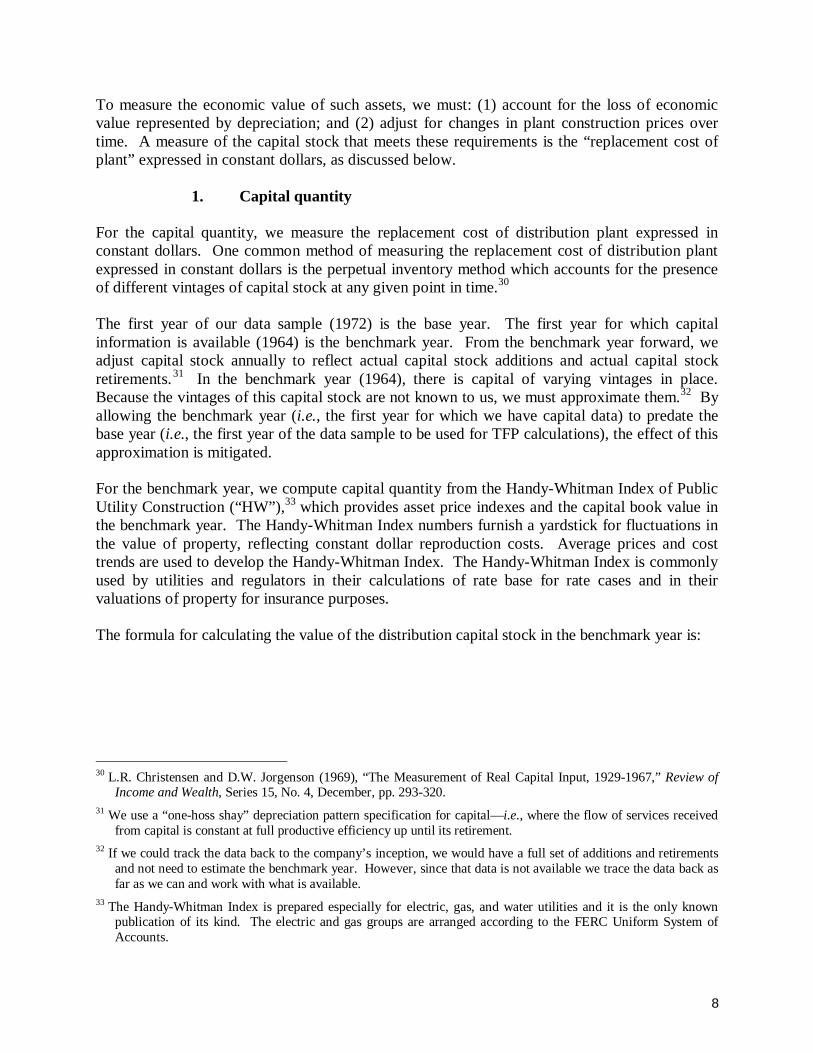
To measure the economic value of such assets, we must: (1) account for the loss of economic value represented by depreciation; and (2) adjust for changes in plant construction prices over time. A measure of the capital stock that meets these requirements is the “replacement cost of plant” expressed in constant dollars, as discussed below.

1. Capital quantity

For the capital quantity, we measure the replacement cost of distribution plant expressed in constant dollars. One common method of measuring the replacement cost of distribution plant expressed in constant dollars is the perpetual inventory method which accounts for the presence of different vintages of capital stock at any given point in time.30

The first year of our data sample (1972) is the base year. The first year for which capital information is available (1964) is the benchmark year. From the benchmark year forward, we adjust capital stock annually to reflect actual capital stock additions and actual capital stock retirements.31 In the benchmark year (1964), there is capital of varying vintages in place. Because the vintages of this capital stock are not known to us, we must approximate them.32 By allowing the benchmark year (i.e., the first year for which we have capital data) to predate the base year (i.e., the first year of the data sample to be used for TFP calculations), the effect of this approximation is mitigated.

For the benchmark year, we compute capital quantity from the Handy-Whitman Index of Public Utility Construction (“HW”),33 which provides asset price indexes and the capital book value in the benchmark year. The Handy-Whitman Index numbers furnish a yardstick for fluctuations in the value of property, reflecting constant dollar reproduction costs. Average prices and cost trends are used to develop the Handy-Whitman Index. The Handy-Whitman Index is commonly used by utilities and regulators in their calculations of rate base for rate cases and in their valuations of property for insurance purposes.

The formula for calculating the value of the distribution capital stock in the benchmark year is:

30 L.R. Christensen and D.W. Jorgenson (1969), “The Measurement of Real Capital Input, 1929-1967,” Review of

Income and Wealth, Series 15, No. 4, December, pp. 293-320. 31 We use a “one-hoss shay” depreciation pattern specification for capital—i.e., where the flow of services received

from capital is constant at full productive efficiency up until its retirement. 32 If we could track the data back to the company’s inception, we would have a full set of additions and retirements

and not need to estimate the benchmark year. However, since that data is not available we trace the data back as far as we can and work with what is available.

33 The Handy-Whitman Index is prepared especially for electric, gas, and water utilities and it is the only known publication of its kind. The electric and gas groups are arranged according to the FERC Uniform System of Accounts.

9

.

HWi

ii

year benchmark in plantutility of value book = K

i

i1

benchmark

+

=

∑∑ 194420

1

20

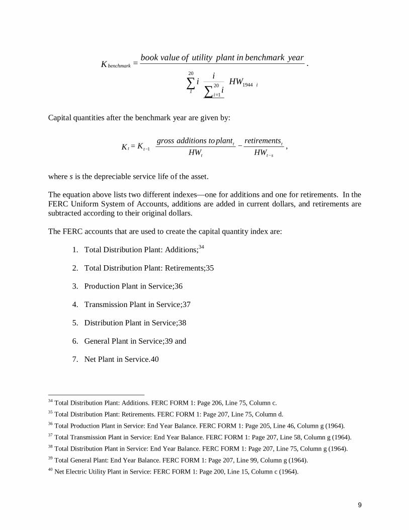
Capital quantities after the benchmark year are given by:

,1 HW

sretirement HW

plantto additions grossK = Kst

t

t

ttt

−− −+

where s is the depreciable service life of the asset.

The equation above lists two different indexes—one for additions and one for retirements. In the FERC Uniform System of Accounts, additions are added in current dollars, and retirements are subtracted according to their original dollars.

The FERC accounts that are used to create the capital quantity index are:

1. Total Distribution Plant: Additions;34

2. Total Distribution Plant: Retirements;35

3. Production Plant in Service;36

4. Transmission Plant in Service;37

5. Distribution Plant in Service;38

6. General Plant in Service;39 and

7. Net Plant in Service.40

34 Total Distribution Plant: Additions. FERC FORM 1: Page 206, Line 75, Column c. 35 Total Distribution Plant: Retirements. FERC FORM 1: Page 207, Line 75, Column d. 36 Total Production Plant in Service: End Year Balance. FERC FORM 1: Page 205, Line 46, Column g (1964). 37 Total Transmission Plant in Service: End Year Balance. FERC FORM 1: Page 207, Line 58, Column g (1964). 38 Total Distribution Plant in Service: End Year Balance. FERC FORM 1: Page 207, Line 75, Column g (1964). 39 Total General Plant: End Year Balance. FERC FORM 1: Page 207, Line 99, Column g (1964). 40 Net Electric Utility Plant in Service: FERC FORM 1: Page 200, Line 15, Column c (1964).

10

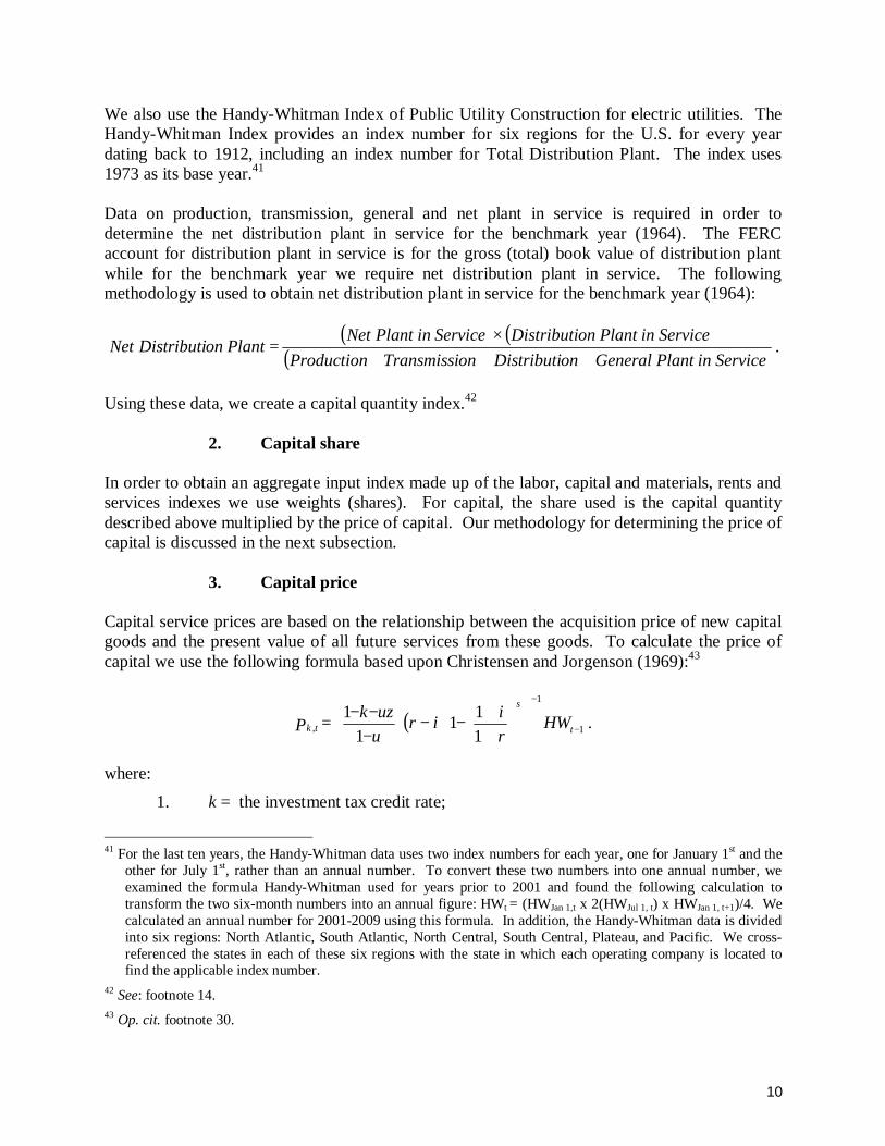
We also use the Handy-Whitman Index of Public Utility Construction for electric utilities. The Handy-Whitman Index provides an index number for six regions for the U.S. for every year dating back to 1912, including an index number for Total Distribution Plant. The index uses 1973 as its base year.41

Data on production, transmission, general and net plant in service is required in order to determine the net distribution plant in service for the benchmark year (1964). The FERC account for distribution plant in service is for the gross (total) book value of distribution plant while for the benchmark year we require net distribution plant in service. The following methodology is used to obtain net distribution plant in service for the benchmark year (1964):

( ) ( )( )ServiceinPlantGeneralonDistributionTransmissioductionPr

ServiceinPlantonDistributiServiceinPlantNetPlantonDistributiNet+++

×= .

Using these data, we create a capital quantity index.42

2. Capital share

In order to obtain an aggregate input index made up of the labor, capital and materials, rents and services indexes we use weights (shares). For capital, the share used is the capital quantity described above multiplied by the price of capital. Our methodology for determining the price of capital is discussed in the next subsection.

3. Capital price

Capital service prices are based on the relationship between the acquisition price of new capital goods and the present value of all future services from these goods. To calculate the price of capital we use the following formula based upon Christensen and Jorgenson (1969):43

( ) . HWriir

uuzk = P t

s

tk 1

1

, 111

11

−

−

++

−−

−−−

where: 1. k = the investment tax credit rate;

41 For the last ten years, the Handy-Whitman data uses two index numbers for each year, one for January 1st and the

other for July 1st, rather than an annual number. To convert these two numbers into one annual number, we examined the formula Handy-Whitman used for years prior to 2001 and found the following calculation to transform the two six-month numbers into an annual figure: HWt = (HWJan 1,t x 2(HWJul 1, t) x HWJan 1, t+1)/4. We calculated an annual number for 2001-2009 using this formula. In addition, the Handy-Whitman data is divided into six regions: North Atlantic, South Atlantic, North Central, South Central, Plateau, and Pacific. We cross-referenced the states in each of these six regions with the state in which each operating company is located to find the applicable index number.

42 See: footnote 14. 43 Op. cit. footnote 30.

11

2. u = the corporate profits tax rate; 3. z = the present value of the depreciation deduction on new investment;

4. r = the cost of capital; 5. i = the expected inflation rate over the lifetime of the assets;

6. s = asset lifetime; and 7. HWt-1 = Handy-Whitman’s asset price in the prior year.

For k, there has been no general investment tax credit for over twenty years.44 For u, the corporate profits tax rate, we obtained information using Form 1120 on the IRS website.45

The present value of future depreciation deductions on new investment, z, is a function of the tax depreciation method used, the asset tax lifetime, and the rate of return. The distinction in asset lives is drawn because depreciation for tax purposes is frequently allowed to take place over a much shorter time span (e.g., five years, or the “sum of the years’ digits” method46) than is allowed for ratemaking purposes. Using the sum of the years’ digits method, z then becomes:

( )( ) ( )

+

−

+

+−

+1

111

1112

T

RTRR

RT =z ,

where R is the rate of return for discounting depreciation deductions and T is the tax lifetime of the asset. In this Study we use a value of 0.511.47

To calculate r, the cost of capital, we used the bond yields of the company’s debt. We obtained monthly long-term bond ratings from Standard & Poor’s (“S&P”) Ratings Direct for each of the

44 The list of all business tax credits can be found at the IRS website for small businesses:

http://www.irs.gov/businesses/small/article/0,,id=99839,00.html, accessed on December 12, 2010. 45 See: IRS publication, "Instructions for Forms 1120 and 1120-A" for each year, available at

http://www.irs.gov/app/picklist/list/priorFormPublication.html, accessed on December 30, 2010. 46 The sum of the years’ digits method is one form of accelerated depreciation. We assign a number to each year of

the asset’s useful life, starting with 1 for the first year, etc. These numbers are added to get their sum, i.e., n(n+1)/2. A separate depreciation rate is then calculated for each year, with the number assignments being reversed. For example, with a 12-year asset life, the sum of the digits is 78. Depreciation in year 1 is then 12/78.

47 See: Makholm Dissertation op. cit footnote 4. Christensen and Jorgenson (1969), op. cit. footnote 30, and Gollop and Jorgenson, “U.S. Productivity Growth by Industry, 1947-1973,” Discussion Paper 7712, Social Systems Research Institute, University of Wisconsin, Madison, September (1977), use a value of R (the rate of return for discounting depreciation deductions) of 0.10. M. Sing (Doctoral Thesis University of Wisconsin 1984), employs a value of T (the tax lifetime of the asset) of 23 years on electric plants. These values give a value of z of 0.511.

12

companies. 48 We then downloaded S&P’s and Moody’s monthly utility bond yields from Bloomberg for Aaa, Aa, A, and Baa ratings.49

To find i, the expected inflation rate over the lifetime of the assets, we obtained data on the Daily Treasury Yield Curve Rates for 30-year bonds from the U.S. Treasury website and averaged them to arrive at a Yearly Treasury Yield Rate (Risk-Free Return).50 To find the Risk-Free Return Net of Inflation, we downloaded the Consumer Price Index from the Bureau of Labor Statistics and subtracted it from the Yearly Treasury Yield Rate for each year from 1972-2009.51 We then averaged this differenced to arrive at the Risk-Free Return Net of Inflation for the period 1972-2009. To find the Expected Long Term Inflation Rate for each year, we subtracted the Risk-Free Return Net of Inflation from the Yearly Treasury Yield Rate.

For s, the asset lifetime, we use 33 years. HWt-1 refers to the same Handy-Whitman Total Distribution Plant asset price index number as that used to calculate the capital index.

V. Results

In this section we present our results for output, inputs and TFP growth.

A. Output Index

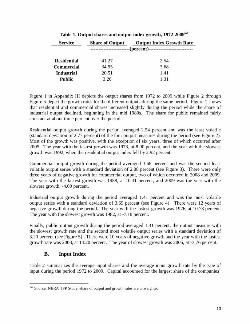
Table 1 summarizes the average output shares and the average output index growth by type of service during the period 1972 to 2009. Residential service comprised the largest component of the firms’ output, followed by commercial, industrial and the public category. The fastest growing output measure was commercial, followed by residential, industrial and the public category.

48 Because S&P did not have a ratings history for Commonwealth Electric, one of the companies that was

consolidated into NSTAR, we found the rating history for that company on Bloomberg. 49 Because Moody’s does not provide yields for anything lower than the Baa rating, we downloaded Fair Value daily

utility bond yields from Bloomberg for the Ba rating. We also downloaded monthly (non-utility specific) junk bond yields from Barclays for the B and D ratings, both of which are non-investment grade. In some instances, the company’s rating was between the ratings provided by Moody’s, such as an A1 rating. In these cases we rounded to the nearest available rating and used the yield for that rating.

50 The Daily Treasury Yield Curve Rates for 30-year bonds were discontinued between February 2002 and February 2006. For this time period, the U.S. Treasury published Daily Treasury Yield Curve Rates for 20-year bonds as well as an “extrapolation factor,” which was designed to be added to the 20-year yield curve rates to estimate 30-year yield curve rates. We therefore used the 20-year yield curve rates plus the extrapolation factor as a substitute for the 30-year yield curve rates between February 2002 and February 2006.

51 Bureau of Labor Statistics, available at: ftp://ftp.bls.gov/pub/special.requests/cpi/cpiai.txt, accessed on December 30, 2010.

13

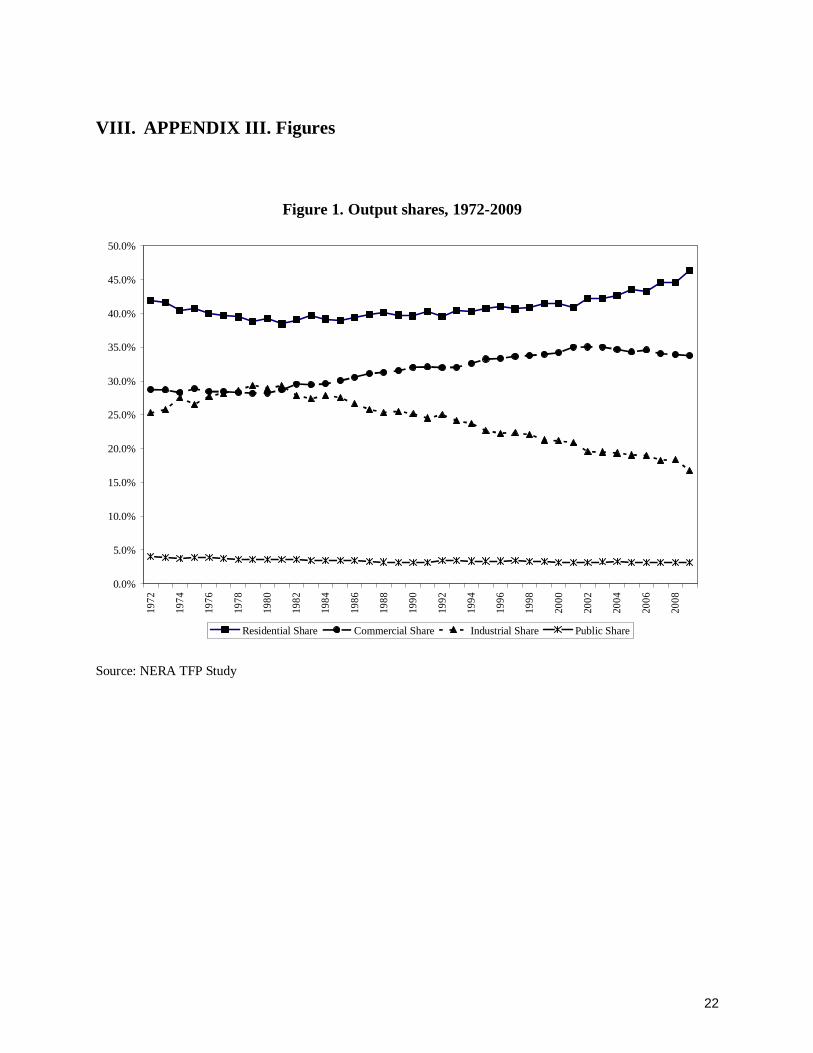
Figure 1 in Appendix III depicts the output shares from 1972 to 2009 while Figure 2 through Figure 5 depict the growth rates for the different outputs during the same period. Figure 1 shows that residential and commercial shares increased slightly during the period while the share of industrial output declined, beginning in the mid 1980s. The share for public remained fairly constant at about three percent over the period.

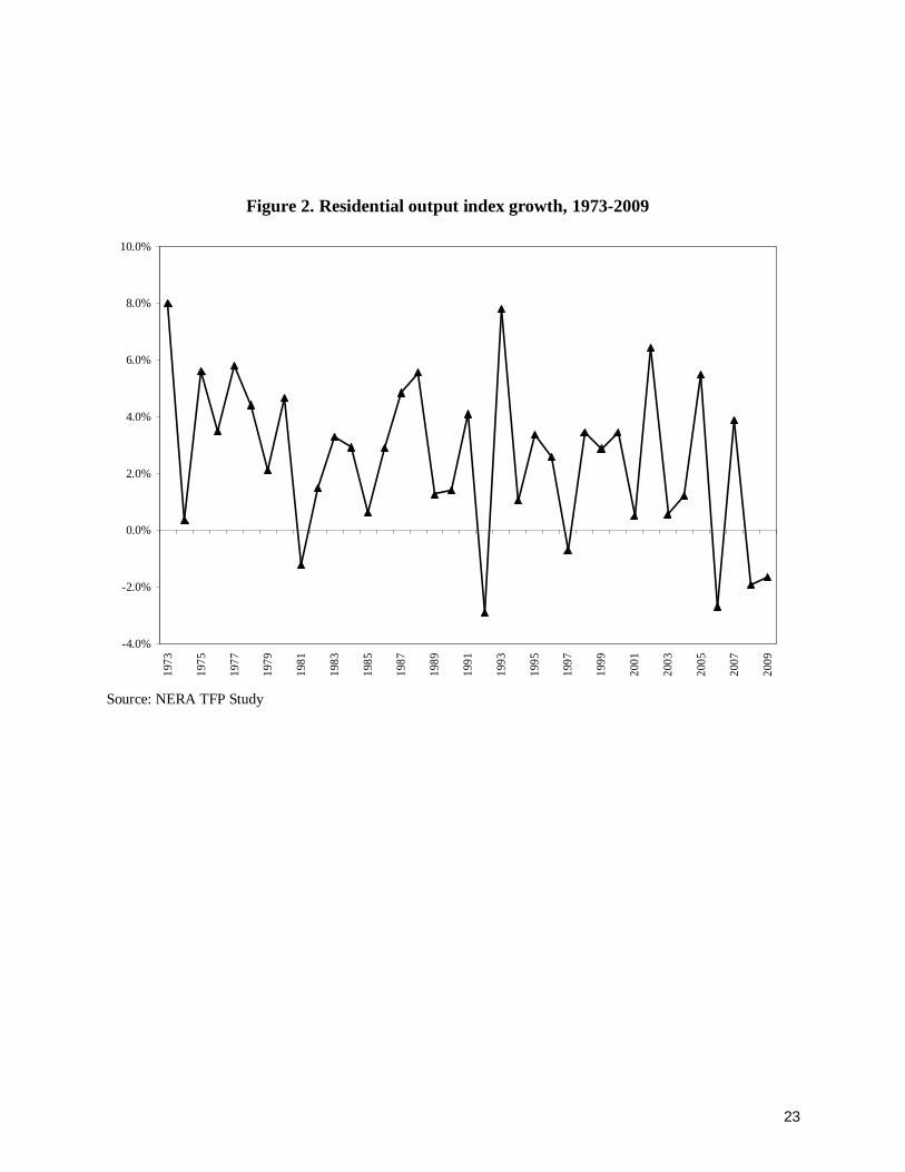
Residential output growth during the period averaged 2.54 percent and was the least volatile (standard deviation of 2.77 percent) of the four output measures during the period (see Figure 2). Most of the growth was positive, with the exception of six years, three of which occurred after 2005. The year with the fastest growth was 1973, at 8.00 percent, and the year with the slowest growth was 1992, when the residential output index fell by 2.92 percent.

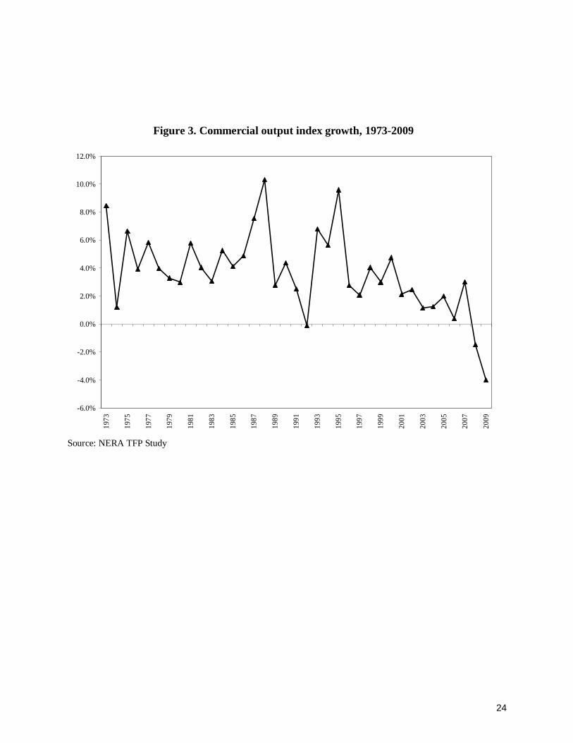
Commercial output growth during the period averaged 3.68 percent and was the second least volatile output series with a standard deviation of 2.88 percent (see Figure 3). There were only three years of negative growth for commercial output, two of which occurred in 2008 and 2009. The year with the fastest growth was 1988, at 10.31 percent, and 2009 was the year with the slowest growth, -4.00 percent.

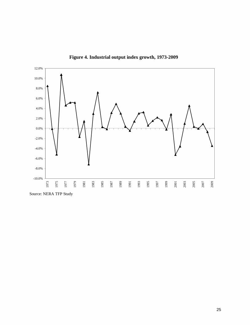
Industrial output growth during the period averaged 1.41 percent and was the most volatile output series with a standard deviation of 3.69 percent (see Figure 4). There were 12 years of negative growth during the period. The year with the fastest growth was 1976, at 10.73 percent. The year with the slowest growth was 1982, at -7.18 percent.

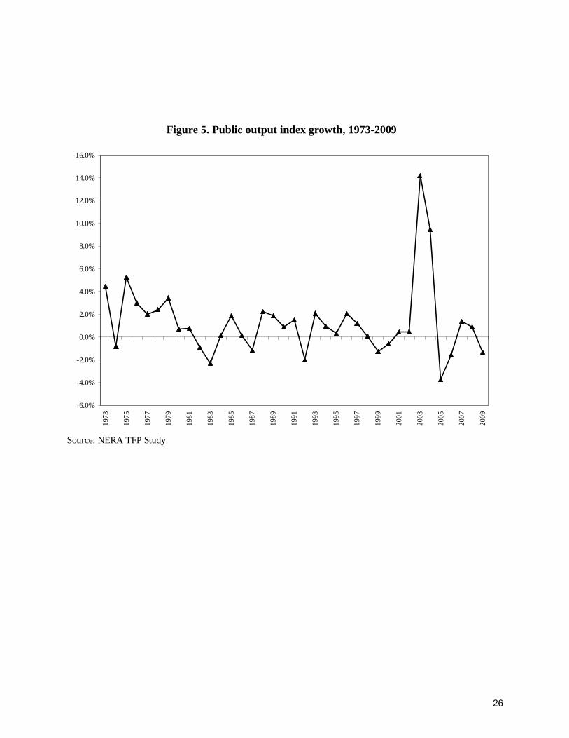
Finally, public output growth during the period averaged 1.31 percent, the output measure with the slowest growth rate and the second most volatile output series with a standard deviation of 3.20 percent (see Figure 5). There were 10 years of negative growth and the year with the fastest growth rate was 2003, at 14.20 percent. The year of slowest growth was 2005, at -3.76 percent.

B. Input Index

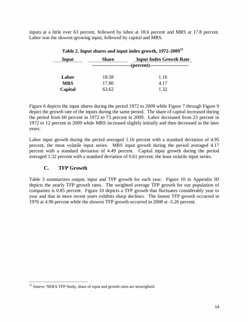
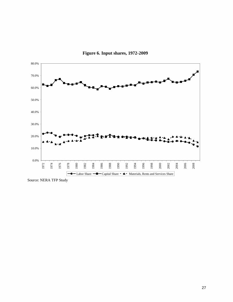
Table 2 summarizes the average input shares and the average input growth rate by the type of input during the period 1972 to 2009. Capital accounted for the largest share of the companies’

52 Source: NERA TFP Study, share of output and growth rates are unweighted.

Table 1. Output shares and output index growth, 1972-200952

Service Share of Output Output Index Growth Rate ------------------------(percent)---------------------------

Residential 41.27 2.54 Commercial 34.95 3.68 Industrial 20.51 1.41

Public 3.26 1.31

14

inputs at a little over 63 percent, followed by labor at 18.6 percent and MRS at 17.8 percent. Labor was the slowest-growing input, followed by capital and MRS.

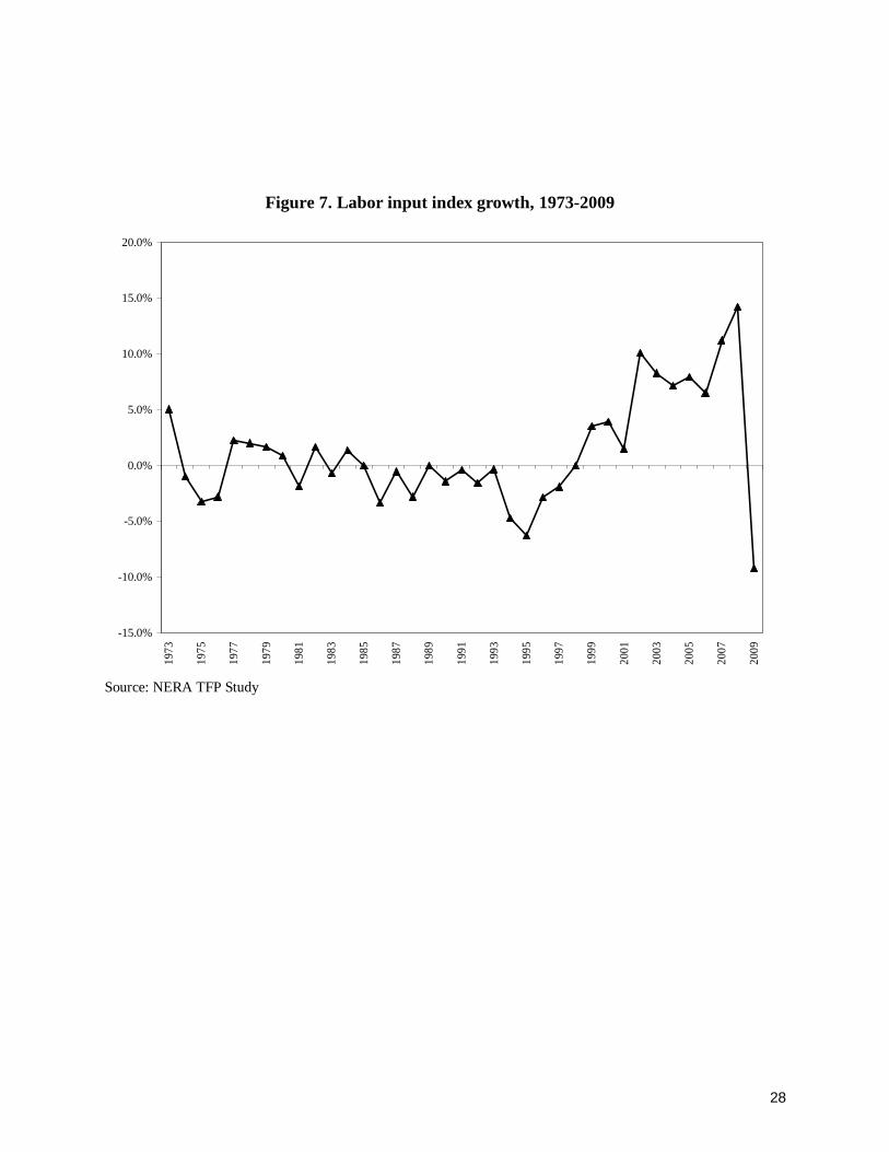
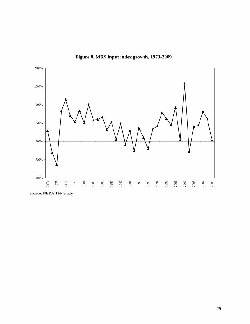
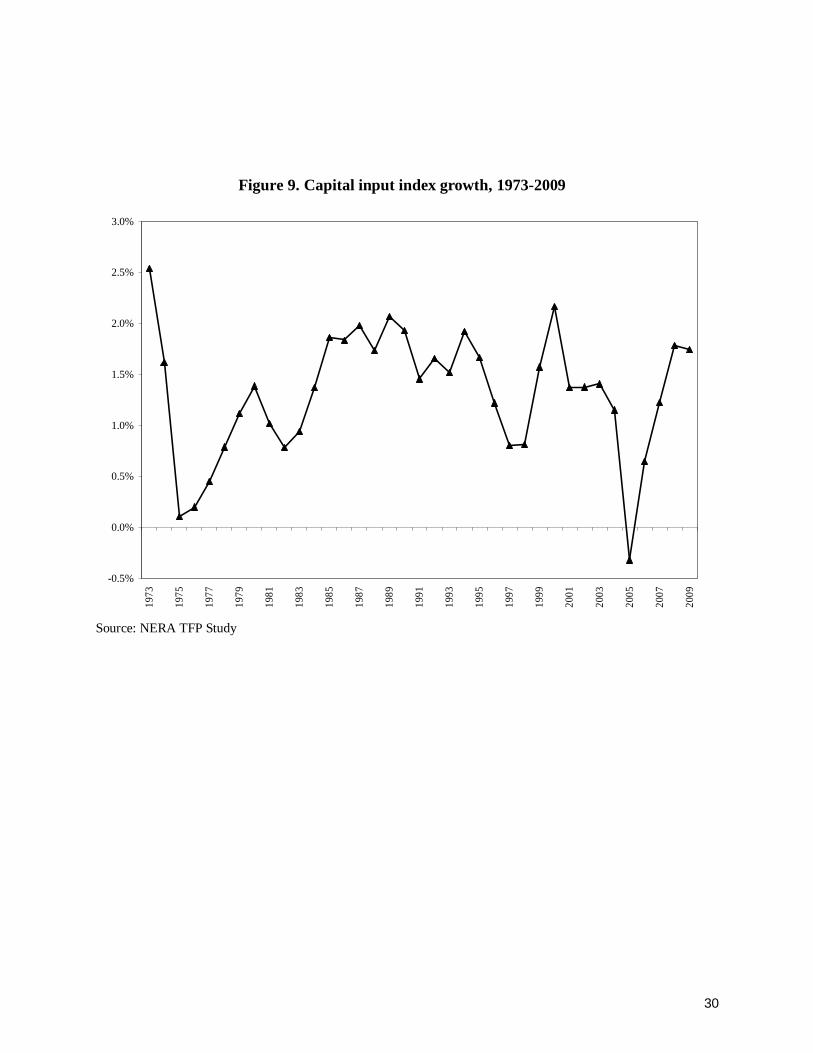
Figure 6 depicts the input shares during the period 1972 to 2009 while Figure 7 through Figure 9 depict the growth rate of the inputs during the same period. The share of capital increased during the period from 60 percent in 1972 to 73 percent in 2009. Labor decreased from 23 percent in 1972 to 12 percent in 2009 while MRS increased slightly initially and then decreased in the later years.

Labor input growth during the period averaged 1.16 percent with a standard deviation of 4.95 percent, the most volatile input series. MRS input growth during the period averaged 4.17 percent with a standard deviation of 4.49 percent. Capital input growth during the period averaged 1.32 percent with a standard deviation of 0.61 percent, the least volatile input series.

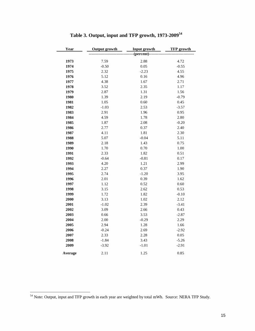
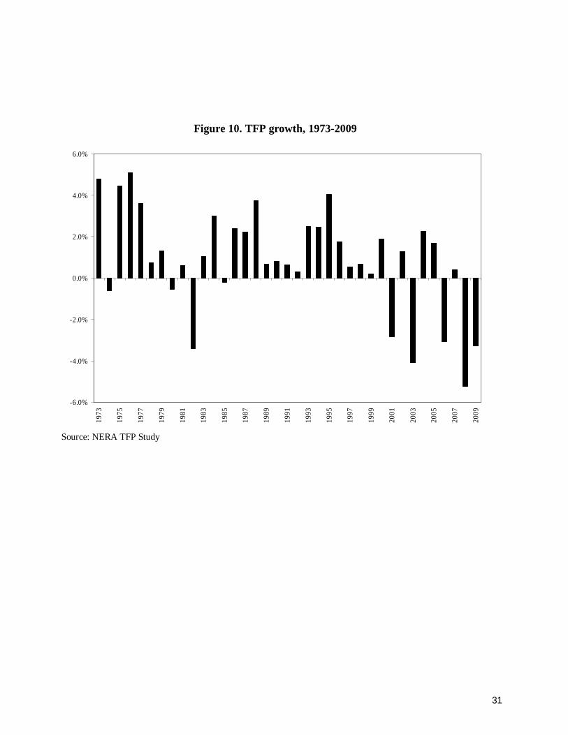
C. TFP Growth

Table 3 summarizes output, input and TFP growth for each year. Figure 10 in Appendix III depicts the yearly TFP growth rates. The weighted average TFP growth for our population of companies is 0.85 percent. Figure 10 depicts a TFP growth that fluctuates considerably year to year and that in more recent years exhibits sharp declines. The fastest TFP growth occurred in 1976 at 4.96 percent while the slowest TFP growth occurred in 2008 at -5.26 percent.

53 Source: NERA TFP Study, share of input and growth rates are unweighted.

Table 2. Input shares and input index growth, 1972-200953

Input Share Input Index Growth Rate ------------------------(percent)------------------------

Labor 18.58 1.16 MRS 17.80 4.17

Capital 63.62 1.32

15

54 Note: Output, input and TFP growth in each year are weighted by total mWh. Source: NERA TFP Study.

Table 3. Output, input and TFP growth, 1973-200954

Year Output growth Input growth TFP growth----------------------------------(percent)----------------------------------

1973 7.59 2.88 4.721974 -0.50 0.05 -0.551975 2.32 -2.23 4.551976 5.12 0.16 4.961977 4.38 1.67 2.711978 3.52 2.35 1.171979 2.87 1.31 1.561980 1.39 2.19 -0.791981 1.05 0.60 0.451982 -1.03 2.53 -3.571983 2.91 1.96 0.951984 4.59 1.78 2.801985 1.87 2.08 -0.201986 2.77 0.37 2.401987 4.11 1.81 2.301988 5.07 -0.04 5.111989 2.18 1.43 0.751990 1.70 0.70 1.001991 2.33 1.82 0.511992 -0.64 -0.81 0.171993 4.20 1.21 2.991994 2.27 0.37 1.901995 2.74 -1.20 3.951996 2.01 0.39 1.621997 1.12 0.52 0.601998 3.15 2.62 0.531999 1.72 1.82 -0.102000 3.13 1.02 2.122001 -1.02 2.39 -3.412002 3.09 2.66 0.432003 0.66 3.53 -2.872004 2.00 -0.29 2.292005 2.94 1.28 1.662006 -0.24 2.69 -2.922007 2.33 2.28 0.052008 -1.84 3.43 -5.262009 -3.92 -1.01 -2.91

Average 2.11 1.25 0.85

16

D. Economy-wide TFP

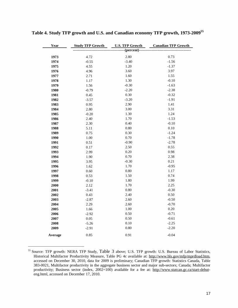
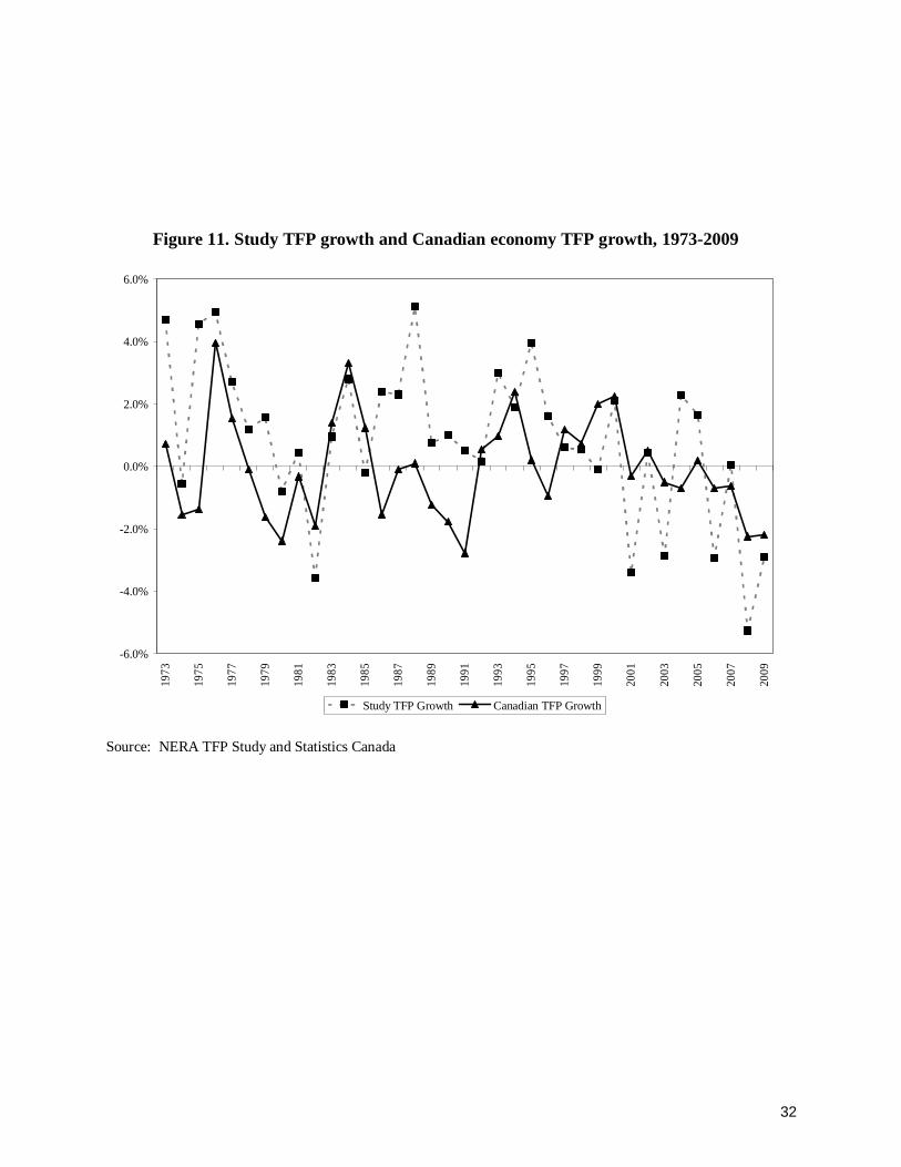
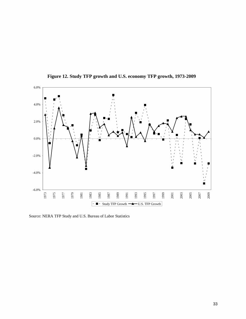
We compare our Study TFP growth to economy-wide productivity. Canadian TFP growth during the 1972 to 2009 period has averaged -0.04 percent. During the same time period U.S. TFP growth has averaged 0.91 percent. Table 4 summarizes the yearly TFP growth rates for the U.S. and Canadian economy vis-à-vis the TFP growth rates in our Study. Figure 11 and Figure 12 compare our Study TFP growth to the TFP growth for the Canadian and U.S. economies, respectively.

17

55 Source: TFP growth: NERA TFP Study, Table 3 above; U.S. TFP growth: U.S. Bureau of Labor Statistics,

Historical Multifactor Productivity Measure, Table PG 4c available at: http://www.bls.gov/mfp/mprdload.htm, accessed on December 30, 2010, data for 2009 is preliminary; Canadian TFP growth: Statistics Canada, Table 383-0021, Multifactor productivity in the aggregate business sector and major sub-sectors; Canada; Multifactor productivity; Business sector (index, 2002=100) available for a fee at: http://www.statcan.gc.ca/start-debut-eng.html, accessed on December 17, 2010.

Table 4. Study TFP growth and U.S. and Canadian economy TFP growth, 1973-200955

Year Study TFP Growth U.S. TFP Growth Canadian TFP Growth------------------------------------------(percent)------------------------------------------

1973 4.72 2.80 0.731974 -0.55 -3.40 -1.561975 4.55 1.20 -1.371976 4.96 3.60 3.971977 2.71 1.60 1.551978 1.17 1.30 -0.101979 1.56 -0.30 -1.631980 -0.79 -2.20 -2.381981 0.45 0.30 -0.321982 -3.57 -3.20 -1.911983 0.95 2.90 1.411984 2.80 3.00 3.311985 -0.20 1.30 1.241986 2.40 1.70 -1.531987 2.30 0.40 -0.101988 5.11 0.80 0.101989 0.75 0.30 -1.241990 1.00 0.70 -1.781991 0.51 -0.90 -2.781992 0.17 2.50 0.551993 2.99 0.20 0.981994 1.90 0.70 2.381995 3.95 -0.30 0.211996 1.62 1.70 -0.951997 0.60 0.80 1.171998 0.53 1.50 0.741999 -0.10 1.80 1.992000 2.12 1.70 2.252001 -3.41 0.80 -0.302002 0.43 2.40 0.502003 -2.87 2.60 -0.502004 2.29 2.60 -0.702005 1.66 1.00 0.202006 -2.92 0.50 -0.712007 0.05 0.50 -0.612008 -5.26 0.10 -2.252009 -2.91 0.80 -2.20

Average 0.85 0.91 -0.04

18

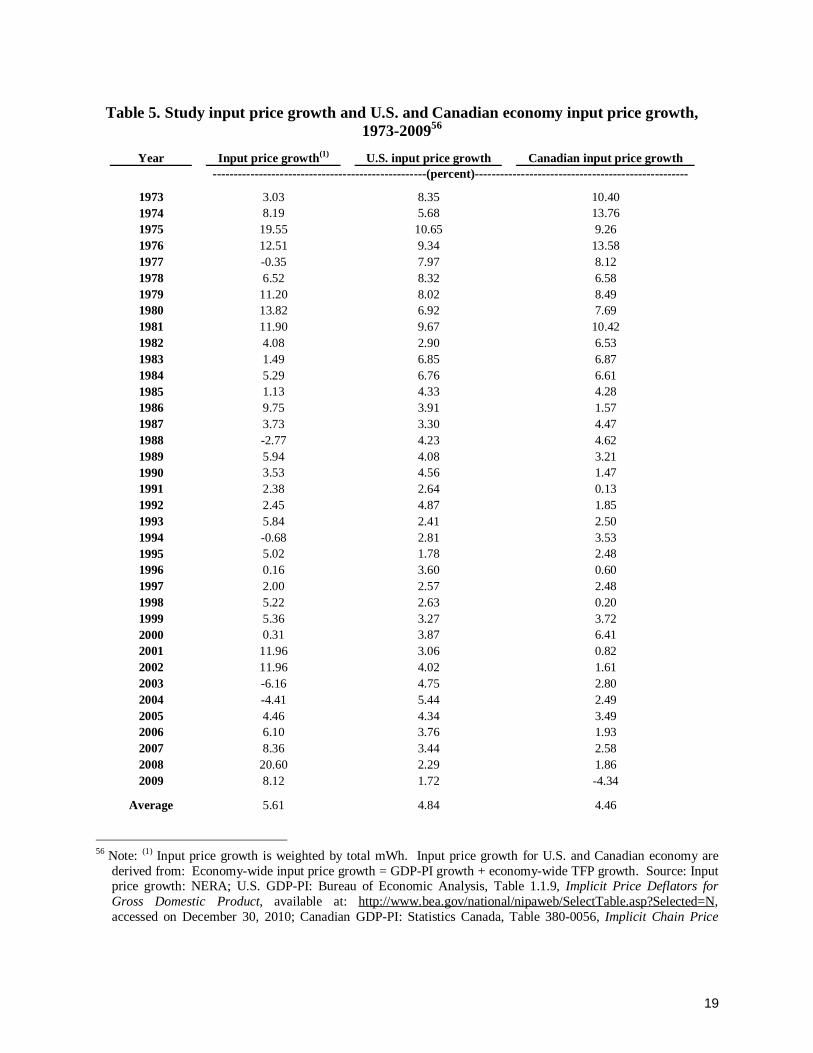
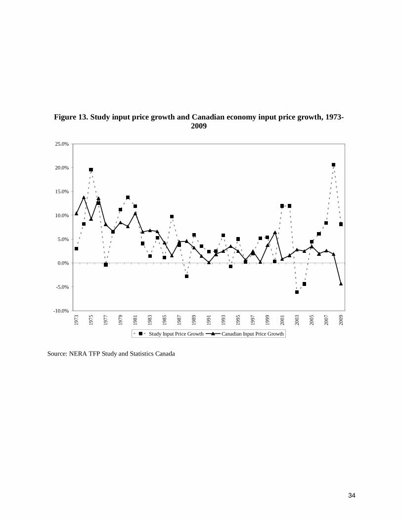
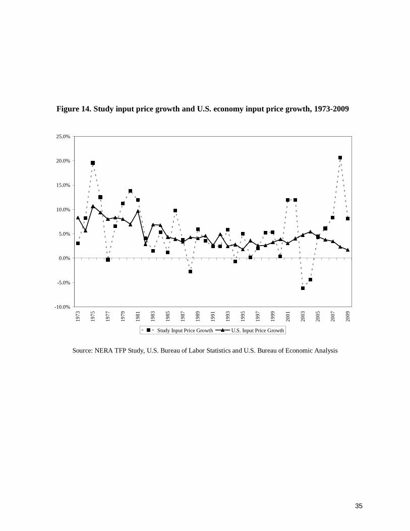
E. Input price growth

We also measured the input price growth during the period 1972 to 2009 and compared it to the input price growth of the Canadian and U.S. economy, respectively. Table 5 summarizes the results. Input prices in our TFP Study grew at an annual rate of 5.61 percent compared to input price growth for the Canadian and U.S. economy of 4.46 percent and 4.84 percent, respectively. Figure 13 compares our Study input price growth to the input price growth for the Canadian economy during the same period while Figure 14 compares our Study input price growth to the input price growth for the U.S. economy during the same period.

We conducted a statistical test to test the hypothesis that there was a statistically significant difference in the input price growth series for our Study and the input price growth series for the Canadian and U.S. economy. Specifically, we estimated the probability associated with a Student’s t-test and rejected the hypothesis that there was a statistically significant difference in the input price growth series for our Study and the input price growth series for the Canadian and U.S. economy.

19

56 Note: (1) Input price growth is weighted by total mWh. Input price growth for U.S. and Canadian economy are

derived from: Economy-wide input price growth = GDP-PI growth + economy-wide TFP growth. Source: Input price growth: NERA; U.S. GDP-PI: Bureau of Economic Analysis, Table 1.1.9, Implicit Price Deflators for Gross Domestic Product, available at: http://www.bea.gov/national/nipaweb/SelectTable.asp?Selected=N, accessed on December 30, 2010; Canadian GDP-PI: Statistics Canada, Table 380-0056, Implicit Chain Price

Table 5. Study input price growth and U.S. and Canadian economy input price growth, 1973-200956

Year Input price growth(1) U.S. input price growth Canadian input price growth---------------------------------------------------(percent)---------------------------------------------------

1973 3.03 8.35 10.401974 8.19 5.68 13.761975 19.55 10.65 9.261976 12.51 9.34 13.581977 -0.35 7.97 8.121978 6.52 8.32 6.581979 11.20 8.02 8.491980 13.82 6.92 7.691981 11.90 9.67 10.421982 4.08 2.90 6.531983 1.49 6.85 6.871984 5.29 6.76 6.611985 1.13 4.33 4.281986 9.75 3.91 1.571987 3.73 3.30 4.471988 -2.77 4.23 4.621989 5.94 4.08 3.211990 3.53 4.56 1.471991 2.38 2.64 0.131992 2.45 4.87 1.851993 5.84 2.41 2.501994 -0.68 2.81 3.531995 5.02 1.78 2.481996 0.16 3.60 0.601997 2.00 2.57 2.481998 5.22 2.63 0.201999 5.36 3.27 3.722000 0.31 3.87 6.412001 11.96 3.06 0.822002 11.96 4.02 1.612003 -6.16 4.75 2.802004 -4.41 5.44 2.492005 4.46 4.34 3.492006 6.10 3.76 1.932007 8.36 3.44 2.582008 20.60 2.29 1.862009 8.12 1.72 -4.34

Average 5.61 4.84 4.46

20

VI. APPENDIX I. List of companies used in the Study

Alabama Power Company Kansas Gas and Electric Company Appalachian Power Company Kentucky Utilities Company Arizona Public Service Company Madison Gas and Electric Company Baltimore Gas and Electric Company Massachusetts Electric Company Carolina Power & Light Company MDU Resources Group, Inc. Central Hudson Gas & Electric Corp Metropolitan Edison Company Central Illinois Light Company Mississippi Power Company Central Vermont Public Service Corporation Monongahela Power Company Cleveland Electric Illuminating Company Narragansett Electric Company Columbus Southern Power Company Nevada Power Company Commonwealth Edison Company New York State Electric & Gas Corp Connecticut Light and Power Company Niagara Mohawk Power Corporation Consolidated Edison Company of New York, Inc. Northern Indiana Public Service Co. Consumers Energy Company NSTAR Dayton Power and Light Company Ohio Edison Company Delmarva Power & Light Company Oklahoma Gas and Electric Company Detroit Edison Company Orange and Rockland Utilities, Inc. Duke Energy Indiana, Inc. Otter Tail Corporation Duke Energy Kentucky, Inc. Pacific Gas and Electric Company Duke Energy Ohio, Inc. PECO Energy Company Duquesne Light Company Pennsylvania Electric Company El Paso Electric Company Portland General Electric Company Empire District Electric Company Public Service Company of Colorado Entergy Arkansas, Inc. Public Service Company of New Hampshire Entergy Gulf States Louisiana, L.L.C. Public Service Electric and Gas Company Entergy Mississippi, Inc. Puget Sound Power and Light Company Entergy New Orleans, Inc. South Carolina Electric & Gas Co. Florida Power & Light Company Southern California Edison Co. Florida Power Corporation Southern Indiana Gas and Elec. Company, Inc. Green Mountain Power Corporation Southwestern Electric Power Company Gulf Power Company Southwestern Public Service Company Idaho Power Company Tucson Electric Power Company Illinois Power Company Virginia Electric and Power Company Indiana Michigan Power Company Western Massachusetts Electric Company Jersey Central Power & Light Company Wisconsin Electric Power Company Kansas City Power & Light Company Wisconsin Public Service Corp

Index Gross Domestic Product, available for a fee at http://www.statcan.gc.ca/start-debut-eng.html, accessed on December 17, 2010.

21

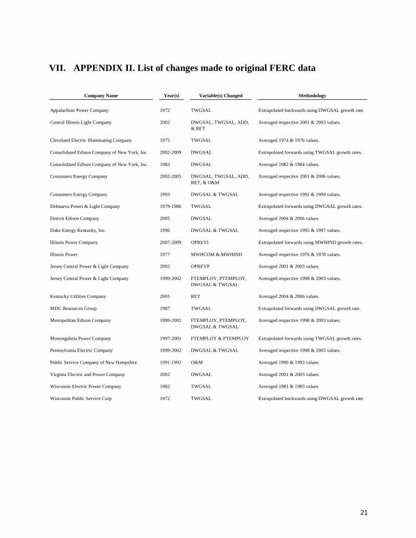
VII. APPENDIX II. List of changes made to original FERC data

Company Name Year(s) Variable(s) Changed Methodology

Appalachian Power Company 1972 TWGSAL Extrapolated backwards using DWGSAL growth rate.

Central Illinois Light Company 2002 DWGSAL, TWGSAL, ADD, & RET

Averaged respective 2001 & 2003 values.

Cleveland Electric Illuminating Company 1975 TWGSAL Averaged 1974 & 1976 values.

Consolidated Edison Company of New York, Inc. 2002-2009 DWGSAL Extrapolated forwards using TWGSAL growth rates.

Consolidated Edison Company of New York, Inc. 1983 DWGSAL Averaged 1982 & 1984 values.

Consumers Energy Company 2002-2005 DWGSAL, TWGSAL, ADD, RET, & O&M

Averaged respective 2001 & 2006 values.

Consumers Energy Company 1993 DWGSAL & TWGSAL Averaged respective 1992 & 1994 values.

Delmarva Power & Light Company 1979-1986 TWGSAL Extrapolated forwards using DWGSAL growth rates.

Detroit Edison Company 2005 DWGSAL Averaged 2004 & 2006 values.

Duke Energy Kentucky, Inc. 1996 DWGSAL & TWGSAL Averaged respective 1995 & 1997 values.

Illinois Power Company 2007-2009 OPREVI Extrapolated forwards using MWHIND growth rates.

Illinois Power 1977 MWHCOM & MWHIND Averaged respective 1976 & 1978 values.

Jersey Central Power & Light Company 2002 OPREVP Averaged 2001 & 2003 values.

Jersey Central Power & Light Company 1999-2002 FTEMPLOY, PTEMPLOY, DWGSAL & TWGSAL

Averaged respective 1998 & 2003 values.

Kentucky Utilities Company 2005 RET Averaged 2004 & 2006 values.

MDU Resources Group 1987 TWGSAL Extrapolated forwards using DWGSAL growth rate.

Metropolitan Edison Company 1999-2002 FTEMPLOY, PTEMPLOY, DWGSAL & TWGSAL

Averaged respective 1998 & 2003 values.

Monongahela Power Company 1997-2001 FTEMPLOY & PTEMPLOY Extrapolated forwards using TWGSAL growth rates.

Pennsylvania Electric Company 1999-2002 DWGSAL & TWGSAL Averaged respective 1998 & 2003 values.

Public Service Company of New Hampshire 1991-1992 O&M Averaged 1990 & 1993 values.

Virginia Electric and Power Company 2002 DWGSAL Averaged 2001 & 2003 values.

Wisconsin Electric Power Company 1982 TWGSAL Averaged 1981 & 1983 values.

Wisconsin Public Service Corp 1972 TWGSAL Extrapolated backwards using DWGSAL growth rate.

22

VIII. APPENDIX III. Figures

Figure 1. Output shares, 1972-2009

0.0%

5.0%

10.0%

15.0%

20.0%

25.0%

30.0%

35.0%

40.0%

45.0%

50.0%

1972

1974

1976

1978

1980

1982

1984

1986

1988

1990

1992

1994

1996

1998

2000

2002

2004

2006

2008

Residential Share Commercial Share Industrial Share Public Share

Source: NERA TFP Study

23

Figure 2. Residential output index growth, 1973-2009

-4.0%

-2.0%

0.0%

2.0%

4.0%

6.0%

8.0%

10.0%

1973

1975

1977

1979

1981

1983

1985

1987

1989

1991

1993

1995

1997

1999

2001

2003

2005

2007

2009

Source: NERA TFP Study

24

Figure 3. Commercial output index growth, 1973-2009

-6.0%

-4.0%

-2.0%

0.0%

2.0%

4.0%

6.0%

8.0%

10.0%

12.0%

1973

1975

1977

1979

1981

1983

1985

1987

1989

1991

1993

1995

1997

1999

2001

2003

2005

2007

2009

Source: NERA TFP Study

25

Figure 4. Industrial output index growth, 1973-2009

-10.0%

-8.0%

-6.0%

-4.0%

-2.0%

0.0%

2.0%

4.0%

6.0%

8.0%

10.0%

12.0%

1973

1975

1977

1979

1981

1983

1985

1987

1989

1991

1993

1995

1997

1999

2001

2003

2005

2007

2009

Source: NERA TFP Study

26

Figure 5. Public output index growth, 1973-2009

-6.0%

-4.0%

-2.0%

0.0%

2.0%

4.0%

6.0%

8.0%

10.0%

12.0%

14.0%

16.0%

1973

1975

1977

1979

1981

1983

1985

1987

1989

1991

1993

1995

1997

1999

2001

2003

2005

2007

2009

Source: NERA TFP Study

27

Figure 6. Input shares, 1972-2009

0.0%

10.0%

20.0%

30.0%

40.0%

50.0%

60.0%

70.0%

80.0%

1972

1974

1976

1978

1980

1982

1984

1986

1988

1990

1992

1994

1996

1998

2000

2002

2004

2006

2008

Labor Share Capital Share Materials, Rents and Services Share

Source: NERA TFP Study

28

Figure 7. Labor input index growth, 1973-2009

-15.0%

-10.0%

-5.0%

0.0%

5.0%

10.0%

15.0%

20.0%

1973

1975

1977

1979

1981

1983

1985

1987

1989

1991

1993

1995

1997

1999

2001

2003

2005

2007

2009

Source: NERA TFP Study

29

Figure 8. MRS input index growth, 1973-2009

-10.0%

-5.0%

0.0%

5.0%

10.0%

15.0%

20.0%

1973

1975

1977

1979

1981

1983

1985

1987

1989

1991

1993

1995

1997

1999

2001

2003

2005

2007

2009

Source: NERA TFP Study

30

Figure 9. Capital input index growth, 1973-2009

-0.5%

0.0%

0.5%

1.0%

1.5%

2.0%

2.5%

3.0%

1973

1975

1977

1979

1981

1983

1985

1987

1989

1991

1993

1995

1997

1999

2001

2003

2005

2007

2009

Source: NERA TFP Study

31

Figure 10. TFP growth, 1973-2009

-6.0%

-4.0%

-2.0%

0.0%

2.0%

4.0%

6.0%

1973

1975

1977

1979

1981

1983

1985

1987

1989

1991

1993

1995

1997

1999

2001

2003

2005

2007

2009

Source: NERA TFP Study

32

Figure 11. Study TFP growth and Canadian economy TFP growth, 1973-2009

-6.0%

-4.0%

-2.0%

0.0%

2.0%

4.0%

6.0%

1973

1975

1977

1979

1981

1983

1985

1987

1989

1991

1993

1995

1997

1999

2001

2003

2005

2007

2009

Study TFP Growth Canadian TFP Growth

Source: NERA TFP Study and Statistics Canada

33

Figure 12. Study TFP growth and U.S. economy TFP growth, 1973-2009

-6.0%

-4.0%

-2.0%

0.0%

2.0%

4.0%

6.0%

1973

1975

1977

1979

1981

1983

1985

1987

1989

1991

1993

1995

1997

1999

2001

2003

2005

2007

2009

Study TFP Growth U.S. TFP Growth

Source: NERA TFP Study and U.S. Bureau of Labor Statistics

34

Figure 13. Study input price growth and Canadian economy input price growth, 1973-2009

-10.0%

-5.0%

0.0%

5.0%

10.0%

15.0%

20.0%

25.0%

1973

1975

1977

1979

1981

1983

1985

1987

1989

1991

1993

1995

1997

1999

2001

2003

2005

2007

2009

Study Input Price Growth Canadian Input Price Growth

Source: NERA TFP Study and Statistics Canada

35

Source: NERA TFP Study, U.S. Bureau of Labor Statistics and U.S. Bureau of Economic Analysis

Figure 14. Study input price growth and U.S. economy input price growth, 1973-2009

-10.0%

-5.0%

0.0%

5.0%

10.0%

15.0%

20.0%

25.0%

1973

1975

1977

1979

1981

1983

1985

1987

1989

1991

1993

1995

1997

1999

2001

2003

2005

2007

2009

Study Input Price Growth U.S. Input Price Growth