Total dissolvable and dissolved iron isotopes in the … · Total dissolvable and dissolved iron...

Available online at www.sciencedirect.com

www.elsevier.com/locate/gca

ScienceDirect

Geochimica et Cosmochimica Acta 162 (2015) 66–82

Total dissolvable and dissolved iron isotopes in the watercolumn of the Peru upwelling regime

Fanny Chever a,b,⇑, Olivier J. Rouxel c, Peter L. Croot d,e,f, Emmanuel Ponzevera c,Kathrin Wuttig d, Maureen Auro g

a Institut Universitaire Europeen de la Mer, Universite de Bretagne Occidentale, 29280 Plouzane, Franceb IFREMER/Centre de Brest, Departement REM/EEP/Laboratoire Environnement Profond, CS 10070, 29280 Plouzane, France

c IFREMER/Centre de Brest, Departement REM/GM/Laboratoire Geochimie et Metallogenie, CS 10070, 29280 Plouzane, Franced GEOMAR Helmholtz Centre for Ocean Research Kiel, Marine Biogeochemistry, Dusternbrooker Weg 20, 24105 Kiel, Germany

e Plymouth Marine Laboratory (PML), Plymouth, Devon, United Kingdomf Earth and Ocean Sciences, School of Natural Sciences, National University of Ireland, Galway, University Road, Galway, Ireland

g Department of Marine Chemistry and Geochemistry, Woods Hole Oceanographic Institute, Woods Hole, MA 02543, USA

Received 5 June 2014; accepted in revised form 17 April 2015; available online 23 April 2015

Abstract

Vertical distributions of iron (Fe) concentrations and isotopes were determined in the total dissolvable and dissolved poolsin the water column at three coastal stations located along the Peruvian margin, in the core of the Oxygen Minimum Zone(OMZ). The shallowest station 121 (161 m total water depth) was characterized by lithogenic input from the continental pla-teau, yielding concentrations as high as 456 nM in the total dissolvable pool. At the 2 other stations (stations 122 and 123), Feconcentrations of dissolved and total dissolvable pools exhibited maxima in both surface and deep layers. Fe isotopic com-position (d56Fe) showed a fractionation toward lighter values for both physical pools throughout the water column for allstations with minimum values observed for the surface layer (between �0.64 and �0.97& at 10–20 m depth) and deep layer(between �0.03 and �1.25& at 160–300 m depth). An Fe isotope budget was established to determine the isotopic compo-sition of the particulate pool. We observed a range of d56Fe values for particulate Fe from +0.02 to �0.87&, with lightestvalues obtained at water depth above 50 m. Such light values in the both particulate and dissolved pools suggest sources otherthan atmospheric dust deposition in the surface ocean, including lateral transport of isotopically light Fe. Samples collected atstation 122 closest to the sediment show the lightest isotope composition in the dissolved and the particulate pools (�1.25 and�0.53& respectively) and high Fe(II) concentrations (14.2 ± 2.1 nM) consistent with a major reductive benthic Fe sourcesthat is transferred to the ocean water column. A simple isotopic model is proposed to link the extent of Fe(II) oxidationand the Fe isotope composition of both particulate and dissolved Fe pools. This study demonstrates that Fe isotopic com-position in OMZ regions is not only affected by the relative contribution of reductive and non-reductive shelf sediment inputbut also by seawater-column processes during the transport and oxidation of Fe from the source region to open seawater.� 2015 Elsevier Ltd. All rights reserved.

http://dx.doi.org/10.1016/j.gca.2015.04.031

0016-7037/� 2015 Elsevier Ltd. All rights reserved.

⇑ Corresponding author at: IFREMER/Centre de Brest,Departement REM/EEP/Laboratoire Environnement Profond,CS 10070, 29280 Plouzane, France. Tel.: +33 2 98 22 45 24.

E-mail address: [email protected] (F. Chever).

1. INTRODUCTION

Iron (Fe) is an essential micronutrient for marine organ-isms (Martin and Fitzwater, 1988). It is now well estab-lished that this element plays a key role in the functioningof the marine ecosystems (Moore et al., 2002; Boyd and


mailto:[email protected]


http://crossmark.crossref.org/dialog/?doi=10.1016/j.gca.2015.04.031&domain=pdf

F. Chever et al. / Geochimica et Cosmochimica Acta 162 (2015) 66–82 67

Ellwood, 2010). In-situ and natural Fe fertilisations havedemonstrated that Fe inputs enhance phytoplanktonbiomass and affect the major biogeochemical cycles (e.g.carbon (C) and nitrogen (N)) (Boyd et al., 2000, 2007;Coale et al., 2004; Jickells et al., 2005; Blain et al., 2007;Pollard et al., 2009). However, the importance of new andregenerated sources of Fe to the water column as well asthe fractions that are truly bioavailable to the phytoplank-ton, are still subject of debate.

Whereas atmospheric deposition was commonlythought to be the predominant external source of Fe inremote areas (Jickells et al., 2005), inputs from sedimentscoupled to upwelling or advection are now considered toprovide significant supply of Fe to surface waters of theopen ocean (Bucciarelli et al., 2001; Elrod et al., 2004;Lam and Bishop, 2008; Tagliabue et al., 2009; Nishiokaet al., 2011). In contrast to the open ocean, shelf environ-ments may receive additional Fe input from fluvial sourcesand sediment resuspension (Croot and Hunter, 1998;Hutchins and Bruland, 1998; Johnson et al., 2001; Elrodet al., 2004; Lam and Bishop, 2008; Lohan and Bruland,2008). Even if Fe supply is significant in those regions, somestudies have shown that, due to the complex physico-chem-ical speciation of Fe in coastal systems, its bioavailabilitycan be limited (Hutchins and Bruland, 1998).

In seawater, Fe occurs in two redox states, Fe(II) andFe(III) (Waite and Morel, 1984). In oxic seawater, the ther-modynamically stable state Fe(III) is highly insoluble (Liuand Millero, 2002) and rapidly hydrolyzes resulting in theprecipitation of various Fe(III) oxyhydroxides. Organicligands complex most of the dissolved Fe in seawater andcontrol the solubility of Fe(III) (Gledhill and van denBerg, 1994; Rue and Bruland, 1995; Millero, 1998;Barbeau et al., 2001; Liu and Millero, 2002; Gledhill andBuck, 2012). Fe(II) is more soluble but is rapidly oxidizedby oxygen (O2) and hydrogen peroxide (H2O2) (Milleroet al., 1987; Millero and Sotolongo, 1989; Gonzalez-Davila et al., 2005; Santana-Casiano et al., 2005; Sarthouet al., 2011). Reduction of Fe(III) to Fe(II) with possiblestabilization by organic ligands is a potential mechanismby which Fe is made more bioavailable to phytoplankton(Anderson and Morel, 1980; Maldonado and Price, 2001).The release of Fe(II) from reducing continental-margin sed-iments (Hong and Kester, 1986; Lohan and Bruland, 2008)as well as Fe(II) supply from seafloor hydrothermal vents(Bennett et al., 2008; Toner et al., 2009; Tagliabue et al.,2010; Wu et al., 2011a; Nishioka et al., 2013; Vedamatiet al., 2014) are now recognized as possible sources ofFe(II) in seawater. Under anoxic conditions as thoseencountered in relatively organic-rich marine sediments,when sulfide generation is limited and thus precluding theprecipitation of FeS minerals reductive dissolution of Feoxides or clay minerals can result in dissolved Fe(II) con-centrations up to 1 mM (Sell and Morse, 2006). In openocean surface waters, the photoreduction of Fe(III) toFe(II) has also been clearly observed (Croot et al., 2008).

The Peruvian coast is characterized by an intensive mid-depth region of low oxygen associated with an upwellingand high surface productivity (Hong and Kester, 1986;Bruland et al., 2005; Stramma et al., 2010). Major changes

to marine sources and sinks of important nutrients such asnitrogen, phosphorus and Fe occur when oceanic oxygenconcentrations decrease below threshold levels (Strammaet al., 2008). Along the continental shelf off the Peruviancoast, labile Fe (i.e. Fe(II)) concentrations up to 73 nMwere attributed to intense redox cycling occurring at thesediment–water interface (Hong and Kester, 1986;Vedamati et al., 2014). This process can result in a greatlyenhanced source of Fe available to upwell to surfacewaters, potentially increasing phytoplankton productivity(Lohan and Bruland, 2008). The Oxygen MinimumZones (OMZs) of the tropics are key regions of low oxygenin today’s ocean. The effects of nutrient cycling under oxy-gen deficient conditions are carried into the rest of theocean by the thermohaline circulation (Stramma et al.,2008). Hence processes occurring in the OMZs, impactingnutrients and Fe cycles, may have an impact on the biolog-ical productivity and carbon cycle of the global ocean(Helly and Levin, 2004; Pennington et al., 2006). Giventhe fact that expansion of the OMZs will continue to occurin the future (Stramma et al., 2008), a better understandingof Fe biogeochemical cycle in those environments is ofgreat interest.

Recent studies of Fe isotopes in open seawater andcoastal regions have shown variability in d56Fe and havedemonstrated how Fe isotopes may be used to constrainthe global Fe cycle. The Fe isotope composition is expressed

by d56Fe defined as: d56Fe ¼ ð56Fe=54FeÞsample

ð56Fe=54FeÞIRMM-14� 1

h i� 103.

Values are reported relative to the IRMM-14 internationaliron isotope reference material (the d56Fe of igneous rocksrelative to IRMM is of +0.09 ± 0.1&, 2SD; Beard et al.,2003a).

In nature, d56Fe variations are mainly controlled byboth biotic and abiotic redox processes along with a rangeof isotope (kinetic and/or equilibrium) fractionations aris-ing from non-redox processes (e.g. Welch et al., 2003;Croal et al., 2004; Johnson et al., 2004; Balci et al., 2006;Dauphas and Rouxel, 2006). Numerous studies were ini-tially led at the ocean boundaries to characterize Fe sourcesto the ocean such as aerosols, sediment porewaters, ground-waters, rivers and hydrothermal vents (Sharma et al., 2001;Severmann et al., 2004, 2006, 2010; Bergquist and Boyle,2006; Rouxel et al., 2008a,b; Bennett et al., 2009; Escoubeet al., 2009; Homoky et al., 2009; Roy et al., 2012). Thosestudies demonstrated that benthic sources of Fe are oftencharacterized with light isotopic values. In the case of ben-thic input from reducing sediments, Fe isotope compositionof pore-fluid at the sediment–seawater interface is highlysensitive to local redox conditions, with most light d56Fevalues being generated through the combination of micro-bial Fe reduction and partial Fe oxidation (Severmannet al., 2006; Homoky et al., 2009). Heavy d56Fe values havebeen also found in anoxic sediment porewater as a result ofthe development of sulfidic conditions and the precipitationof isotopically light Fe sulfides (Severmann et al., 2006; Royet al., 2012). Homoky et al. (2013) recently highlighted theimportance of the ‘non-reductive’ dissolution of continentalmargin sediments as a source of dissolved Fe in seawaterthat is characterized by d56Fe values close to crustal values.

5°S

6°S

5°30

’S

81°30’W 81°W 80°30’W82°W

Rio Chira

Rio Sechura

121

122123

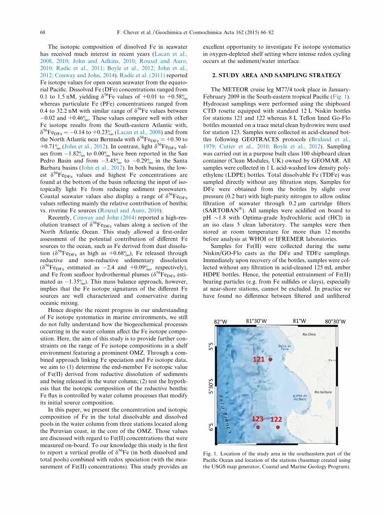
Fig. 1. Location of the study area in the southeastern part of thePacific Ocean and location of the stations (basemap created usingthe USGS map generator, Coastal and Marine Geology Program).

68 F. Chever et al. / Geochimica et Cosmochimica Acta 162 (2015) 66–82

The isotopic composition of dissolved Fe in seawaterhas received much interest in recent years (Lacan et al.,2008, 2010; John and Adkins, 2010; Rouxel and Auro,2010; Radic et al., 2011; Boyle et al., 2012; John et al.,2012; Conway and John, 2014). Radic et al. (2011) reportedFe isotope values for open ocean seawater from the equato-rial Pacific. Dissolved Fe (DFe) concentrations ranged from0.1 to 1.5 nM, yielding d56Fe values of +0.01 to +0.58&

whereas particulate Fe (PFe) concentrations ranged from0.4 to 32.2 nM with similar range of d56Fe values between�0.02 and +0.46&. These values compare well with otherFe isotope results from the South-eastern Atlantic with,d56FeDFe = �0.14 to +0.23& (Lacan et al., 2008) and fromthe North Atlantic near Bermuda with d56FeDFe = +0.30 to+0.71& (John et al., 2012). In contrast, light d56FeDFe val-ues from �1.82& to 0.00& have been reported in the SanPedro Basin and from �3.45& to �0.29& in the SantaBarbara basins (John et al., 2012). In both basins, the low-est d56FeDFe values and highest Fe concentrations arefound at the bottom of the basin reflecting the input of iso-topically light Fe from reducing sediment porewaters.Coastal seawater values also display a range of d56FeDFe

values reflecting mainly the relative contribution of benthicvs. riverine Fe sources (Rouxel and Auro, 2010).

Recently, Conway and John (2014) reported a high-res-olution transect of d56FeDFe values along a section of theNorth Atlantic Ocean. This study allowed a first-orderassessment of the potential contribution of different Fesources to the ocean, such as Fe derived from dust dissolu-tion (d56FeDFe as high as +0.68&), Fe released throughreductive and non-reductive sedimentary dissolution(d56FeDFe estimated as �2.4 and +0.09&, respectively),and Fe from seafloor hydrothermal plumes (d56FeDFe esti-mated as �1.35&). This mass balance approach, however,implies that the Fe isotope signatures of the different Fesources are well characterized and conservative duringoceanic mixing.

Hence despite the recent progress in our understandingof Fe isotope systematics in marine environments, we stilldo not fully understand how the biogeochemical processesoccurring in the water column affect the Fe isotope compo-sition. Here, the aim of this study is to provide further con-straints on the range of Fe isotope compositions in a shelfenvironment featuring a prominent OMZ. Through a com-bined approach linking Fe speciation and Fe isotope data,we aim to (1) determine the end-member Fe isotopic valueof Fe(II) derived from reductive dissolution of sedimentsand being released in the water column; (2) test the hypoth-esis that the isotopic composition of the reductive benthicFe flux is controlled by water column processes that modifyits initial source composition.

In this paper, we present the concentration and isotopiccomposition of Fe in the total dissolvable and dissolvedpools in the water column from three stations located alongthe Peruvian coast, in the core of the OMZ. Those valuesare discussed with regard to Fe(II) concentrations that weremeasured on-board. To our knowledge this study is the firstto report a vertical profile of d56Fe (in both dissolved andtotal pools) combined with redox speciation (with the mea-surement of Fe(II) concentrations). This study provides an

excellent opportunity to investigate Fe isotope systematicsin oxygen-depleted shelf setting where intense redox cyclingoccurs at the sediment/water interface.

2. STUDY AREA AND SAMPLING STRATEGY

The METEOR cruise leg M77/4 took place in January-February 2009 in the South-eastern tropical Pacific (Fig. 1).Hydrocast samplings were performed using the shipboardCTD rosette equipped with standard 12 L Niskin bottlesfor stations 121 and 122 whereas 8 L Teflon lined Go-Flobottles mounted on a trace metal clean hydrowire were usedfor station 123. Samples were collected in acid-cleaned bot-tles following GEOTRACES protocols (Bruland et al.,1979; Cutter et al., 2010; Boyle et al., 2012). Samplingwas carried out in a purpose built class 100 shipboard cleancontainer (Clean Modules, UK) owned by GEOMAR. Allsamples were collected in 1 L acid-washed low density poly-ethylene (LDPE) bottles. Total dissolvable Fe (TDFe) wassampled directly without any filtration steps. Samples forDFe were obtained from the bottles by slight overpressure (0.2 bar) with high-purity nitrogen to allow onlinefiltration of seawater through 0.2 lm cartridge filters(SARTOBAN�). All samples were acidified on board topH �1.8 with Optima-grade hydrochloric acid (HCl) inan iso class 5 clean laboratory. The samples were thenstored at room temperature for more than 12 monthsbefore analysis at WHOI or IFREMER laboratories.

Samples for Fe(II) were collected during the sameNiskin/GO-Flo casts as the DFe and TDFe samplings.Immediately upon recovery of the bottles, samples were col-lected without any filtration in acid-cleaned 125 mL amberHDPE bottles. Hence, the potential entrainment of Fe(II)bearing particles (e.g. from Fe sulfides or clays), especiallyat near-shore stations, cannot be excluded. In practice wehave found no difference between filtered and unfiltered

0

50

100

150

200

250

300

350

400

450

0 50 100 150 200 250

Dep

th(m

)

[O2] (µM)

121122123

11

12

13

14

15

16

17

1834.80 34.90 35.00 35.10

Tem

pera

ture

(°C

)

Salinity (‰)

121122123

(a) (b)

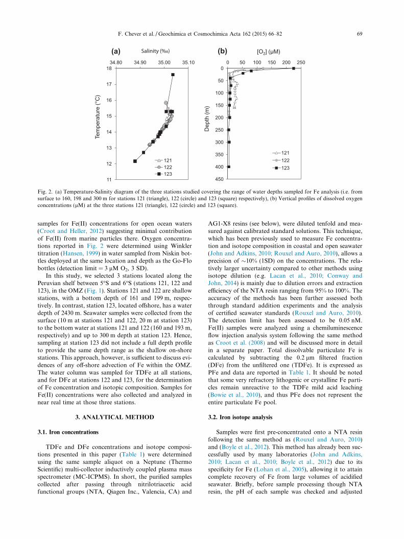
Fig. 2. (a) Temperature-Salinity diagram of the three stations studied covering the range of water depths sampled for Fe analysis (i.e. fromsurface to 160, 198 and 300 m for stations 121 (triangle), 122 (circle) and 123 (square) respectively), (b) Vertical profiles of dissolved oxygenconcentrations (lM) at the three stations 121 (triangle), 122 (circle) and 123 (square).


samples for Fe(II) concentrations for open ocean waters(Croot and Heller, 2012) suggesting minimal contributionof Fe(II) from marine particles there. Oxygen concentra-tions reported in Fig. 2 were determined using Winklertitration (Hansen, 1999) in water sampled from Niskin bot-tles deployed at the same location and depth as the Go-Flobottles (detection limit = 3 lM O2, 3 SD).

In this study, we selected 3 stations located along thePeruvian shelf between 5�S and 6�S (stations 121, 122 and123), in the OMZ (Fig. 1). Stations 121 and 122 are shallowstations, with a bottom depth of 161 and 199 m, respec-tively. In contrast, station 123, located offshore, has a waterdepth of 2430 m. Seawater samples were collected from thesurface (10 m at stations 121 and 122, 20 m at station 123)to the bottom water at stations 121 and 122 (160 and 193 m,respectively) and up to 300 m depth at station 123. Hence,sampling at station 123 did not include a full depth profileto provide the same depth range as the shallow on-shorestations. This approach, however, is sufficient to discuss evi-dences of any off-shore advection of Fe within the OMZ.The water column was sampled for TDFe at all stations,and for DFe at stations 122 and 123, for the determinationof Fe concentration and isotopic composition. Samples forFe(II) concentrations were also collected and analyzed innear real time at those three stations.

3. ANALYTICAL METHOD

3.1. Iron concentrations

TDFe and DFe concentrations and isotope composi-tions presented in this paper (Table 1) were determinedusing the same sample aliquot on a Neptune (ThermoScientific) multi-collector inductively coupled plasma massspectrometer (MC-ICPMS). In short, the purified samplescollected after passing through nitrilotriacetic acidfunctional groups (NTA, Qiagen Inc., Valencia, CA) and

AG1-X8 resins (see below), were diluted tenfold and mea-sured against calibrated standard solutions. This technique,which has been previously used to measure Fe concentra-tion and isotope composition in coastal and open seawater(John and Adkins, 2010; Rouxel and Auro, 2010), allows aprecision of �10% (1SD) on the concentrations. The rela-tively larger uncertainty compared to other methods usingisotope dilution (e.g. Lacan et al., 2010; Conway andJohn, 2014) is mainly due to dilution errors and extractionefficiency of the NTA resin ranging from 95% to 100%. Theaccuracy of the methods has been further assessed boththrough standard addition experiments and the analysisof certified seawater standards (Rouxel and Auro, 2010).The detection limit has been assessed to be 0.05 nM.Fe(II) samples were analyzed using a chemiluminescenceflow injection analysis system following the same methodas Croot et al. (2008) and will be discussed more in detailin a separate paper. Total dissolvable particulate Fe iscalculated by subtracting the 0.2 lm filtered fraction(DFe) from the unfiltered one (TDFe). It is expressed asPFe and data are reported in Table 1. It should be notedthat some very refractory lithogenic or crystalline Fe parti-cles remain unreactive to the TDFe mild acid leaching(Bowie et al., 2010), and thus PFe does not represent theentire particulate Fe pool.

3.2. Iron isotope analysis

Samples were first pre-concentrated onto a NTA resinfollowing the same method as (Rouxel and Auro, 2010)and (Boyle et al., 2012). This method has already been suc-cessfully used by many laboratories (John and Adkins,2010; Lacan et al., 2010; Boyle et al., 2012) due to itsspecificity for Fe (Lohan et al., 2005), allowing it to attaincomplete recovery of Fe from large volumes of acidifiedseawater. Briefly, before sample processing though NTAresin, the pH of each sample was checked and adjusted

Table 1Fe(II), DFe, PFe and TDFe concentrations and d56Fe values in the water column of Stations 121, 122 and 123 from the Peru margin.

Depth(m)

Fe(II)(nM)

DFe(nM)

d56FeDFe

2SD TDFe(nM)

d56FeTDFe

2SD PFe*

(nM)2SD d56Fe

PFe$2SD$ Fe(II)/

DFeFe(II)/TDFe

Fe(II)/PFe

DFe/TDFe

D d56Fe(PFe–DFe)£

2SD

Station 121 (5�10.010 S; 81�21.020 W; 161 m water depth)10 0.24 – – – 14.6 �0.81 0.06 – – – – 0.02 – – – –50 0.34 – – – 115 �0.24 0.04 – – – – 0.00 – – – –

100 1.3 – – – 456 0.04 0.04 – – – – 0.00 – – – –154 6.3 – – – 201 0.01 0.04 – – – – 0.03 – – – –157 7.0 – – – 191 �0.04 0.04 – – – – 0.04 – – – –160 7.7 – – – 197 �0.03 0.04 – – – – 0.04 – – – –

Station 122 (6�0.010 S; 81�15.440 W; 198 m water depth)10 0.59 7.3 �0.68 0.06 32.9 �0.64 0.04 25.6 4.0 �0.63 0.09 0.08 0.02 0.02 0.22 0.05 0.1150 0.39 4.1 �0.32 0.12 7.3 �0.40 0.06 3.2 1.1 �0.51 0.38 0.09 0.05 0.12 0.56 �0.19 0.40

100 1.4 7.8 �0.83 0.12 29.2 �0.54 0.04 21.4 3.7 �0.44 0.15 0.18 0.05 0.06 0.27 0.39 0.19187 12.2 15.0 �1.08 0.06 63.4 �0.52 0.04 48.4 7.8 �0.35 0.11 0.81 0.19 0.25 0.24 0.73 0.12190 16.4 15.4 �1.15 0.06 62.8 �0.58 0.04 47.3 7.8 �0.39 0.08 1.00 0.26 0.35 0.25 0.76 0.10193 14.2 15.0 �1.25 0.06 59.2 �0.53 0.04 44.1 7.4 �0.29 0.09 0.94 0.24 0.32 0.25 0.96 0.11

Station 123 (5�59.990 S; 81�30.090 W; 2430 m water depth)20 1.05 5.4 �0.97 0.12 14.3 �0.91 0.06 9.0 2.0 �0.87 0.26 0.20 0.07 0.12 0.38 0.10 0.2950 0.83 2.5 �0.43 0.12 3.7 �0.66 0.12 <DL – – – – – – – – –80 0.83 1.9 �0.71 0.11 7.7 �0.29 0.06 5.8 1.0 �0.15 0.18 0.43 0.11 0.14 0.25 0.56 0.21

120 0.93 2.0 �0.60 0.11 7.3 �0.15 0.06 5.3 0.9 0.02 0.21 0.46 0.13 0.17 0.28 0.62 0.24200 1.23 1.9 �0.31 0.11 4.4 �0.21 0.12 2.5 0.6 �0.13 0.42 0.63 0.28 0.50 0.44 0.18 0.43250 2.25 3.0 �0.66 0.12 22.8 �0.36 0.04 19.8 2.6 �0.32 0.09 0.75 0.10 0.11 0.13 0.34 0.15300 2.59 2.8 �0.47 0.12 24.0 �0.34 0.04 21.2 2.7 �0.32 0.07 0.92 0.11 0.12 0.12 0.15 0.14

Bold values refer to isotope composition data discussed in the text.Concentration DFe and PFe data are given with a precision of 10%.– ‘not determined’.<DL: below detection limits.

* Total dissolvable particles (PFe) have been calculated subtracting the DFe to the TDFe. Precision is given.$ Fe isotope composition of PFe has been calculated using isotope mass balance relationships between DFe and PFe. Error (2SD) has been obtained after error propagation.£ Fe isotope fractionation factor D d56Fe * (PFe � DFe) determined as d56Fe PFe � d56Fe DFe.

70F

.C

hever

etal./

Geo

chim

icaet

Co

smo

chim

icaA

cta162

(2015)66–82


using ultra-clean HCl (optima grade, Fisher) to obtain a pHbetween 1.7 and 1.8. Hydrogen peroxide (30% v/v Optimagrade, Fisher) was then added to a concentration of1 mL/L to oxidize any ferrous Fe present in the sampleprior to sample processing. The NTA resin was packed intoacid-cleaned chromatographic columns (Poly-Prep col-umns, Bio-Rad Inc.) with a wet volume of 1.8 mL. Priorto sample loading, the resin was resuspended and rinsedwith 25 mL of a 0.7 M nitric acid (HNO3) + 0.6 M HClmixture followed by 50 mL of 18.2 MO-cm purified wateracidified to pH 1.8 with ultra-clean HCl. Between 900 and950 mL of water sample were passed through the NTAchromatographic columns and the remaining volume wasarchived. A peristaltic pump operating at a constant flowrate between 2.5 and 5 mL/min was used to slowly drawthe samples through the chromatographic columns. Afterthe water sample was passed through the resin, 15 mL ofpH 1.8 Milli-Q water was used to elute the remaining sam-ple matrix from the column walls and resin. Fe was finallyeluted with 7 mL of 1.4 M HNO3, recovered in acid-cleaned8 mL polytetrafluoroethylene (PTFE) vials and evaporatedon an all-Teflon hot plate. Evaporated samples were thenredissolved in 6 M HCl for further purification throughAG1-X8 (Bio-Rad, Inc.) anion resin following previouslyestablished methods (e.g. Rouxel et al., 2008b; Escoubeet al., 2009).

Analyzes of 56Fe/54Fe and 57Fe/54Fe ratios were carriedout using a Thermo Scientific Neptune MC-ICP-MS atIFREMER (Brest, France). The medium mass resolutionmode was used to resolve isobaric interferences, such as40Ar16O+ on 56Fe+, 40Ar16O1H+ on 57Fe+, and 40Ar14N+

on 54Fe+ (Weyer and Schwieters, 2003). Two blocks of 25integrations of 4 s were measured. Samples were introducedinto the plasma torch using an Apex-Q introduction system(Elemental Scientific) and a PFA micro-concentric nebulizeroperating at a flow rate of about 60 ll min�1. The Apex-Qsystem increases the instrument sensitivity by a factor of 5relative to conventional spray chambers. The instrumentsensitivity was further improved using X-cones whichresulted in a �twofold increase of instrument sensitivity rel-ative to normal cones. 54Fe, 56Fe, 57Fe, 60Ni and 62Ni iso-tope signals were acquired simultaneously on Faradaycups. Baseline corrections were made before acquisition ofeach data block by completely deflecting the ion beam.Although separated, isobaric Cr interference was alwayschecked and corrected during all analysis, using theNeptune’s peak jumping mode on 52Cr mass. A standardbracketing approach, which normalizes the Fe isotope ratioto the average measured composition of a standard(IRMM-14) was carried out before and after each sample.All sample and standard solutions were diluted with0.28 M ultra-clean HNO3 (Optima Grade, Fisher) in appro-priate concentrations so that the bracketing standard (i.e.IRMM-14) had approximately the same concentration asthe sample (±10%). Instrumental mass bias was correctedusing an internal Ni standard (SRM 986). The two methodscombined permit higher precision and the verification of anyinstrumental artefacts generated by residual matrix ele-ments. The internal precision of the data at 95% confidencelevels reported in Table 1 were calculated based on the

analysis of the bracketing standards. Analyses were carriedout using 2–3 mL of Fe solutions. The pure IRMM-14 stan-dard gave a d56Fe external precision of 0.04–0.13& (2r) forFe concentrations ranging from 400 to 70 ppb, respectively.We also used an internal Fe standard provided by NIST(SRM3126a) which yielded d56Fe values of +0.42 ± 0.07&

(2r, n = 10) relative to IRMM-14. This value is indistin-guishable, within uncertainty, from its nominal d56Fe valueof +0.39& (Rouxel and Auro, 2010). This standard is usedas external control of instrumental accuracy and is used rou-tinely throughout the entire chemical purification proce-dure. We also measured d57Fe values, but the values aregenerally less precise due to lower 57Fe abundances relativeto 56Fe. Since the relationship between d56Fe and d57Fe ofthe samples plots on a mass fractionation line, only d56Fevalues are discussed in this paper.

4. RESULTS

4.1. Hydrography

The temperature–salinity (T–S) diagram for the depthssampled for Fe analysis is plotted in Fig. 2a. The three sta-tions are composed of the same water masses, with a mixingof a surface layer (S > 35.0 and T > 15 �C) with a deeperwater mass (S < 34.7 and T < 10 �C). Potential differencesobserved between the vertical profiles cannot thus beexplained by differences in water masses.

Surface waters are characterized by dissolved oxygenconcentrations ranging from 57 lM (station 121) to225 lM (station 123) (Fig. 2b). Below the surface layer,O2 concentrations decrease sharply, reaching hypoxic con-centrations at just 10 m depth at stations 121 and 122 (23and 35 lM) and at 70 m at station 123 (11 lM). Bottomwater O2 concentrations of 23 and 4 lM were observed atstations 121 and 122, respectively. At the offshore station123, O2 concentration rapidly decreased to concentrations<10 lM below 40 m, reaching a minimum of 5 lM at300 m depth. In previous study areas of benthic Fe supplyled along the California Borderland Basins, similarly lowbottom O2 concentration of 3–4 lM have been alreadyreported (Severmann et al., 2010). In the same area as ours,Hong and Kester (1986) and Noffke et al. (2012) alsoobserved vertical O2 concentrations decreasing from morethan 200 to less than 10 lM from the surface to the bottomwaters. By comparison, in the hypoxic shelf waters offOregon and Washington, Lohan and Bruland (2008)observed a minimum oxygen concentration of 43 lMwithin the bottom boundary layer whereas Severmannet al. (2010) measured bottom water oxygen concentrationsranging between 30 and 50 lM along the southern Oregoncoast.

4.2. Vertical distribution of Fe and d56Fe

4.2.1. Iron concentrations

Vertical distributions of Fe are plotted in Fig. 3, whileconcentrations are reported in Table 1. In the total dissolv-able pool, the highest concentrations were observed at sta-tion 121. At this station, TDFe (Fig. 3a) concentrations

Dep

th (m

)

(a) (b) (c) (d)

0

50

100

150

200

250

300

350

0 10 20DFe (nM)

122123

0

50

100

150

200

250

300

350

0 20 40 60PFe (nM)

122123

0

50

100

150

200

250

300

350

0 10 20Fe(II) (nM)

121

122

123

0

50

100

150

200

250

300

350

0 100 200 300 400 500TDFe (nM)

123

121

122

Fig. 3. Vertical profiles of (a) total dissolvable Fe (TDFe), (b) dissolved Fe (DFe), (c) total dissolvable particles (PFe = TDFe � DFe) and (d)Fe(II) concentrations (nM) at stations 121 (triangle), 122 (circle) and 123 (square).


increased from the surface to 100 m (with values rangingfrom 14.6 to 456 nM) before decreasing to a bottom con-centration of 200 nM at 160 m. At stations 122 and 123, amaximum of TDFe was observed in the surface layer withvalues of 32.9 nM and 14.3 nM, respectively and a mini-mum was reached for both stations at 50 m (TDFe of 7.3and 3.7 nM at stations 122 and 123 respectively).Concentrations increased then with depth. At the station122, TDFe concentrations reached 61.8 ± 2.3 nM (1SD,n = 3) in the deepest water, 12 m above the seafloor. At sta-tion 123, located off the coast, TDFe concentrationsincreased to 24.0 nM at 300 m.

DFe vertical profiles followed the same trend as TDFeones (Fig. 3b and Table 1). A maximum was observed inthe surface layer, with values of 7.3 and 5.4 nM at stations122 and 123, respectively and a minimum was reached at50 m at station 122 with 4.1 nM. At station 122, DFe con-centrations also increased close to the sediment, with valuesreaching 15.2 ± 0.3 nM (1SD, n = 3) in the deepest water,12 m above the seafloor. At station 123, DFe concentra-tions increased to 3.0 nM below 250 m depth.

Vertical distributions of PFe (Fig. 3c) follow the sametrend as the DFe and TDFe. At station 122, PFe representsbetween 73% and 78% of the total Fe pool except at 50 mwhere it represented 44%. The same trend was observedat station 123, with particles representing 76 ± 14%(n = 7) of the total pool except at 50 m where it represented31%. The predominance of the particulate phase near con-tinental margin was already observed in numerous studies(Hong and Kester, 1986; Johnson et al., 1999; Chaseet al., 2005; Lohan and Bruland, 2008).

Such TDFe and DFe concentrations are in agreementwith previous studies led in coastal areas of the PacificOcean. Hong and Kester (1986) observed high total Fe con-centrations at coastal stations located near the Peruviancoasts with values reaching 533 nM at 15 m depth. In thebenthic boundary layer off Washington and Oregon,

Lohan and Bruland (2008) measured labile particulate Feconcentrations (defined by the leaching of the >0.4 lm par-ticulate samples) that reached 162 ± 25 nM. DFe concen-trations increased with depth until reaching 50 nM in thebottom water, which was also observed in the same regionby Bruland et al. (2005).

At the two shallowest stations, high Fe(II) concentrationswere encountered (Table 1 and Fig. 3d). Concentrationsincreased with depth, reaching maximum bottom values of7.72 and 16.40 nM at stations 121 and 122 respectively. Atstation 123, Fe(II) concentrations were lower. A maximumwas reached at 300 m ([Fe(II)] = 2.59 nM), where DFe andTDFe enrichment was also observed. As those depths arein the core of the OMZ, the supply of Fe is probably dueto advection from the shelf region. In a recent studyVedamati et al. (2014) also found elevated Fe(II) in bottomwaters along transects across continental shelf in the centraland southern sectors of the Peruvian coast with the offshorestations of the transects often having a mid water Fe(II)maxima coincident with the secondary nitrite maximum.

4.2.2. Iron isotopes

Vertical profiles of Fe isotopes in the total dissolvableand dissolved pools (d56FeTDFe and d56FeDFe, respectively)are plotted in Fig. 4a, b and data are reported in Table 1.For the three stations, either in the total dissolvable orthe dissolved pool, values are isotopically light relative toIRMM-14.

For all the stations, a minimum was observed in the sur-face layer with values ranging from �0.64& (station 122) to�0.91& (station 123) in the total dissolvable pool and from�0.68& (station 122) to �0.97& (station 123) in thedissolved pool (Table 1). Those surface d56Fe values areeven lighter than values observed below in the water col-umn. Several authors already highlighted light Fe isotopiccomposition in the surface layer (John and Adkins, 2010;Rouxel and Auro, 2010; John et al., 2012). However, other

0

50

100

150

200

250

300

350

-1.00 -0.50 0.00 0.50δ56Fe TDFe (‰)

123

121

122

0

50

100

150

200

250

300

350

-1.50 -1.00 -0.50 0.00 0.50δ56Fe PFe (‰)

123

122

0

50

100

150

200

250

300

350

-1.50 -0.50 0.50δ56Fe DFe (‰)

123

122

Dep

th (m

)

(a) (b) (c) (d)

0

50

100

150

200

250

300

350

-0.50 0.00 0.50 1.00 1.50Δδ56Fe PFe-DFe (‰)

123

122

Fig. 4. Vertical profiles of Fe isotope compositions in the (a) total dissolvable (TDFe), (b) dissolved (DFe) and (c) total dissolvable particles(PFe) pools at stations 121 (triangle), 122 (circle) and 123 (square) (in&). (d) represents the isotope fractionation factor between dissolved andparticulate Fe pool defined as Dd56FePFe–DFe = d56FePFe � d56FeDFe.


studies have also reported heavy compositions (Lacanet al., 2010; Radic et al., 2011). The environment wherethose stations were located (coastal or open ocean) as wellas the sources of Fe and the processes controlling its cyclemost likely explain the range of values measured.

Below the surface layer, the distribution of Fe isotopesin the dissolved and the total dissolvable pools is variablebut remains light (d56Fe from �0.03& to �1.25&). Closeto the bottom, the dissolved pool exhibits a minimum (i.e.at station 122) with d56Fe values down to �1.25&.Between 187 and 193 m, d56Fe values ranged from�1.08& to �1.25&. Such light values at the sediment–wa-ter interface have already been highlighted by severalauthors (Severmann et al., 2006, 2010; John et al., 2012).

At stations 122 and 123, knowing the proportion andthe isotopic composition of DFe and TDFe, an Fe isotopebudget can be established in order to estimate the isotopiccomposition of the dissolvable particulate phase, usingthe following mass balance Eq. (1):

d56FeTDFe ¼ XDFe � d56FeDFe þXPFe � d56FePFe ð1Þ

where XDFe and XPFe are the relative proportion of dis-solved and particulate Fe (PFe = TDFe � DFe). Verticalprofiles of calculated d56Fe values for PFe (d56FePFe) areplotted in Fig. 4c together with uncertainties determinedby error propagation using the Monte Carlo (i.e. stochasticsimulation) method also reported in Table 1. The resultsshow that d56FePFe values are all isotopically light withinuncertainties. At station 122, d56FePFe values range from�0.63 ± 0.10& (10 m) to �0.29 ± 0.12& (193 m) and atstation 123, they are in the range of �0.87 ± 0.91&

(20 m) to +0.02 ± 0.20& (120 m). The Fe isotope fraction-ation between dissolved and particulate Fe pool, defined asDd56FePFe–DFe = d56FePFe � d56FeDFe is positive withinerrors (Fig. 4d and Table 1), with values ranging from+0.05 ± 0.15& (10 m, Station 122) to +0.96 ± 0.18&

(193 m, station 122). Due to low concentrations of PFe in

several samples at Station 122 (50 m) and Station 123 (50,200 m), Dd56FePFe–DFe values could not be calculated accu-rately after error propagation (Table 1). Those samples willnot be including in the later discussion pertaining to partic-ulate Fe pool.

5. DISCUSSION

5.1. Surface waters

Several sources could explain the Fe enrichment in DFeand TDFe observed in the surface layer at stations 121 and122. First, atmospheric deposition and riverine inputs arecommonly considered the dominant surface sources of Fein coastal areas (Jickells et al., 2005). It has been shown thataerosols display d56Fe values indistinguishable from thecrustal value defined as �0.09& (Beard et al., 2003b;Waeles et al., 2007). Hence, the light d56Fe values observedfor TDFe at our three stations (Table 1) suggest that dustdeposition cannot explain light d56Fe values. For compar-ison, DFe isotope composition in the North Atlantic, a typ-ical region with high dust deposition, yields relativelyhomogeneous and heavy d56Fe values throughout the watercolumn (between +0.30& and +0.45&) (John et al., 2012).It has been demonstrated that Fe delivered from eolian dustflux accounts for less than a few percent of the Fe requiredfor the observed productivity in the Peru upwelling regime(Fung et al., 2000; Bruland et al., 2005). Considering fur-ther the south-eastern trade winds observed in this area(Fung et al., 2000), we suggest that the observed Fe enrich-ment in surface water is not related to dust deposition.

Total Fe carried by rivers, including both dissolved andsuspended fractions, has variable d56Fe values rangingessentially from +0.5& to �1& suggesting that riverineinput may, in some cases, be characterized by isotopicallylight d56Fe values relative to igneous rocks (Fantle andDePaolo, 2004; Bergquist and Boyle, 2006; Escoube et al.,


2009; Schroth et al., 2011; Poitrasson et al., 2014). The lar-gest river draining to the Pacific in South America, theGuayas River and the Guayaquil estuary in Ecuador, arelocated about 350 km north from Station 121 and 450 kmfrom Stations 122 and 123. Minor freshwater input between5� and 6�S include the Chira and Sechura-Piura riversdraining terrains of the northern desert of Peru. Althoughthis area was in a la Nina or ENSO-neutral stage at the timethe samples were collected, the salinity profiles at the threestations (Fig. 2) indicate that there is no freshwater input insurface water, either from river or groundwater input.Hence, it is unlikely that freshwater input could explainthe light d56Fe values of surface water that are observedin all stations.

Other mechanisms may potentially explain the light val-ues observed in both particulate and dissolved Fe pools. Inthe surface layer, heterotroph bacteria are known to pro-duce low-molecular weight ferric-specific chelators (sidero-phores) in Fe-depleted marine environments (Wilhelm andTrick, 1994) that allow the dissolution of Fe oxyhydroxideand lithogenic particles. Hence, Fe isotope fractionation insurface seawater can potentially be attributed to Fe-organicligand complexation and non-congruent dust dissolution,as recently suggested by Conway and John (2014).Experimental determination of the equilibrium isotopefractionation factor between Fe(III) bound to siderophoreand the dissolved inorganic Fe complex suggest enrichmentin heavier Fe isotopes in the organic complexes (Dideriksenet al., 2008; Morgan et al., 2010), which is opposite of themeasured d56FeDFe in the Peruvian system (Fig. 4).Another potential mechanism explaining light d56FeDFe val-ues in the surface layer is from biological fractionation pro-cesses as previously suggested by de Jong et al. (2007). Inthe Bothnian Sea, Staubwasser et al. (2013) explained heav-ier surface d56FeDFe values by biological uptake due to thepresence of a cyanobacterial bloom, and in the EquatorialPacific Ocean, Radic et al. (2011) hypothesized that phyto-plankton would favor the uptake of light Fe isotopes andthat the surrounding waters would get heavier as they getdepleted. In the Peru upwelling regime, large diatoms tendto dominate the biomass in phytoplankton blooms thatdevelop (Wilkerson et al., 2000; Bruland et al., 2005).Those diatom communities could thus play an importantrole in controlling the Fe isotope fractionation between dis-solved and particulate pools.

Despite the current limited knowledge of the biogeo-chemical processes affecting Fe isotopes in seawater, simpleisotopic mass balance consideration between DFe andTDFe suggests that the overall source of Fe to the upperocean in all stations is isotopically light. As shown inFig. 4d, Dd56FePFe–DFe values at 10–20 m depth forStations 122 and 123 are between +0.05& and +0.1&, thusidentical within uncertainty. The lack of Fe isotope frac-tionation between dissolved and particulate Fe in the upperwater column also preclude the identification of potentialFe isotope fractionation through photochemical reactions.Fe(II) concentrations in surface waters were 0.24, 0.59and 1.05 nM at stations 121, 122 and 123 respectively.Such concentrations could be reached with photoredoxcycling of particulate phases. Indeed, previous studies

showed that photoreduction of Fe(III) (oxyhydroxides, col-loids and particles) and photolysis of organic, colloidal andparticulate Fe are processes that occur in surface water(Waite and Morel, 1984; Kuma et al., 1992; Barbeauet al., 2001; Rijkenberg et al., 2006; Croot et al., 2008).Wiederhold et al. (2006) observed that Fe isotopes arefractionated during reductive dissolution of Fe oxidespromoted by photochemical processes. Enrichment of lightisotopes in the dissolved phase was observed.

Based on our current understanding of Fe isotope frac-tionation both photoreduction and ligand-promoted disso-lution could explain the low d56FeDFe values measured inthe surface waters but not in the particulate pool(Table 1). We propose that the most plausible explanationfor both light and similar d56FePFe and d56FeDFe in the sur-face layer is the advection and transport of isotopically lightFe from shallower near-shore sediments. The light d56FePFe

values measured in the Baltic Sea were hypothesized tocome from water diffusing up from the basin margin sedi-ments after suboxic early-diagenetic remineralization(Gelting et al., 2010; Staubwasser et al., 2013). Along thePeru margin, water masses within the OMZ show a signif-icant enrichment in Fe(II) which may be later oxidized toFe(III) as it is upwelled or laterally transported within oxy-genated surface waters. This freshly formed Fe(III) poolwould then record the light signature of Fe(II) when reach-ing the surface, explaining the light isotopic signatureobserved in the PFe pool. Processes arising in benthic zoneor in intermediate water masses can thus have an impact onthe isotopic composition observed in surface waters, asexplained in paragraph 5.3 below, using a simple isotopicmodel.

5.2. Benthic source

In coastal environments, sediments are an importantsource of Fe to the water column (Hutchins and Bruland,1998; Elrod et al., 2004). Along the Peruvian coasts, lowlevels of dissolved oxygen increase the rate of benthic fluxesand the amount of Fe(II) escaping from the sediments. Atthe bottom of station 122, the DFe pool is dominated byFe(II) (Table 1) (between 81% and 100%) and reaches15 nM, which is a typical benthic value of hypoxic condi-tions over the continental shelf (Lohan and Bruland,2008). To our knowledge, it is the first time that the redoxspeciation was determined at the same time as the isotopiccomposition in the water column. Our results clearly indi-cate that isotopically light DFe between �0.5& and�1.2& released from the Peruvian margin is almost entirelyin the form of Fe(II), with Fe(II)/DFe above 0.8.

Several techniques have previously been used to deter-mine the isotopic signature of the Fe originated from thesediment: porewater measurements, benthic chamber mea-surements or model (Severmann et al., 2006, 2010; Johnet al., 2012). In all those studies, an isotopically lightd56Fe signature of the sedimentary dissolved Fe of around�3& near the sediment–water interface has been deter-mined. Biotic processes involving redox changes arethought to explain the largest Fe isotope fractionationsobserved in marine sediment porewaters (Johnson et al.,


2008). Among those processes, reduction of Fe(III) by dis-similatory Fe-reducing bacteria (process known as dissimi-latory iron reduction “DIR”) is considered to beresponsible for large shifts in isotope compositions (downto �3&) (Crosby et al., 2007; Homoky et al., 2009).However, other mechanisms such as indirect reduction ofFe(III) by sulfide from microbial sulfate reduction, isotopicre-equilibration between Fe(II) and Fe(III) near the sedi-ment–water interface, and partial Fe(II) re-oxidation mayalso combine to produce such light isotopic values of ben-thic Fe(II) fluxes (Rouxel et al., 2008b; Severmann et al.,2010; John et al., 2012). In particular, John et al. (2012)suggested that the invariance in dissolved d56Fe measuredby different techniques reflect a single process (rapidFe(II)–Fe(III) isotopic equilibration) setting a characteristi-cally light d56Fe values for the flux from all reducing conti-nental margin sediment. Hence, it can be considered thatabiotic Fe redox cycling may contribute to most of Fe iso-tope fractionation. Regardless of the mechanisms of Fe iso-tope fractionation, our results confirm the existence of anisotopically light benthic Fe source.

The lowest d56FeDFe values (�1.16 ± 0.09&, 1SD,n = 3) found in the deepest water at Station 122, 12 mabove the seafloor are in the same range as those measuredin the San Pedro basin (from �1.1& to �1.8&) (Johnet al., 2012) but higher than the mean values ��3&

reported by (Severmann et al., 2010) for DFe at the sedi-ment/water interface. As shown in Fig. 5a, the d56Fe valuesfor Fe(II) (i.e. when Fe(II)/DFe � 1) estimated at Station123 is about �0.5&. The results suggest either (i) a substan-tial variation of the end-member isotopic composition ofFe(II) released from the sediments in our study area, forexample due to the development of sulfidic conditions inthe surface sediment driving the porewater isotope compo-sition to heavier values (Severmann et al., 2006; Roy et al.,2012); (ii) the isotopic composition of DFe (and Fe(II))released from sediments has been modified during its advec-tion off-shore.

Regardless of the processes controlling the supply andFe isotope signatures from benthic sediments, the data alsopoint out the importance of water-column processes

(a)

-1.40

-1.20

-1.00

-0.80

-0.60

-0.40

-0.20

0.00

0.00 0.50 1.00

δ56 F

eD

Fe

Fe(II) / DFe

123

122

Fig. 5. The relationship between (a) Fe(II)/DFe and d56FeDFe and betweeand 123 (square).

affecting Fe signatures of the dissolved and particulatepool, as discussed below. An important observation is thatFe isotopic composition of particles associated with isotopi-cally light Fe(II) is heavier, yielding systematically positiveDd56FePFe–DFe values up to +0.96 ± 0.18& in the suboxicwater column. The maximum enrichment in heavy Fe iso-topes in the particulate Fe pool is observed for the maxi-mum Fe(II) enrichment at depth, which is consistent withredox-driven Fe isotope fractionation. It is now widelyreported, both theoretically and experimentally, that partialFe(II) oxidation produces isotopically heavy Fe(III) oxides(e.g. Bullen et al., 2001; Welch et al., 2003; Dauphas andRouxel, 2006; Wu et al., 2011b). A maximum Dd56FePFe–

DFe values of about +0.96& is similar to Fe isotopefractionation during Fe(II) oxidation and precipitation offerrihydrite (Bullen et al., 2001), but lower than predicteddissolved Fe(III)–Fe(II) equilibrium isotope effect of 3.4&

at 6.5 �C (Welch et al., 2003). Additional experimentalwork has also determined the equilibrium Fe isotope frac-tionation factors between Fe(III) hydrous oxide andFe(II)aq of up to 3.2& (Wu et al., 2011b) reflecting funda-mental differences in bonding environments and/or kineticisotopic effects during natural ferrihydrite precipitation.Adsorption of isotopically heavier Fe (Icopini et al., 2004;Teutsch et al., 2005) onto Fe(III) particles and close vs.open system behavior during oxidative Fe precipitationmay also affect observed Dd56FePFe–DFe values (Dauphasand Rouxel, 2006). In all cases, the sign ofDd56FePFe–DFe > 0& is opposite to the isotope fractiona-tion found between dissolved and particulate Fe in the sub-oxic part of the water column in the Baltic Sea, EasternGotland Basin (Staubwasser et al., 2013). Together withprevious studies of Fe isotope fractionation during Fe(II)oxidation in subterranean estuaries (Rouxel et al., 2008b),our result suggest that ferrihydrite precipitation should leadto the enrichment in heavy isotopes relative to Fe(II) inmarine environments, with a range of fractionation factorscontrolled by isotope exchange kinetics and mineral phases.

As shown in Fig. 5b, Dd56FePFe–DFe values are corre-lated with Fe(II)/PFe ratios over the entire profile forStation 122 and 123. This suggests a strong relationship

(b)

R² = 0.7474

-0.40

-0.20

0.00

0.20

0.40

0.60

0.80

1.00

1.20

0.00 0.10 0.20 0.30 0.40

Δδ56

Fe P

Fe-D

Fe

Fe(II) / PFe

123

122

n (b) Dd56FePFe–DFe and the ratio Fe(II)/PFe at stations 122 (circle)


between the relative amount of Fe(II) oxidized in the watercolumn and Fe isotope composition. A preliminary Fe iso-tope model is presented below.

5.3. Chemical modeling of Fe speciation and isotope

composition

DFe in seawater, which is operationally defined as Fethat passes through a 0.2 lm or 0.45 lm filter, can be com-posed of several pools of Fe that are interacting with eachother. A schematic presentation of such Fe pools togetherwith major biogeochemical processes is presented inFig. 6. The predominant form of DFe, noted as DFe(III)-L, is Fe(III) strongly bound to organic ligands (Rue andBruland, 1995). DFe generally includes organic and inor-ganic colloidal forms of Fe (i.e. size range between0.02 lm to 0.2 lm), which may represent up to 80–90% ofDFe in near-surface waters and 30–70% in deep water,the remainder being defined as truly soluble Fe (Wuet al., 2001). As discussed above, DFe in OMZ such asthe Peru margin may also be composed of Fe(II) (referredas DFe(II)) (Millero and Sotolongo, 1989; Croot et al.,2001; Lohan and Bruland, 2008) which can itself be stabi-lized by organic ligands. The large range of Fe(II)/DFeratios obtained in the water column of the Peru margin(Fig. 7), from <0.1 to nearly 1, together with high DFe con-centrations suggests that all of these pools are present.Similarly, PFe may include several pools of Fe, including

DFe(III)-L PFe(III)

DFe(II)56Fe~

-1.2‰56Fe~ δδ0‰

PFe(litho+bio)

Sediment

Bottom water

Surface water Uptake / precipitation

Dissolution

Desorption / Reduction

Adsorption / Oxidation

Reductive sedimentary dissolution

Non reductive sediment dissolution and resuspension

Atmospheric Deposition

Fig. 6. Simplified schematic interpretation of processes affectingthe distribution and exchange of the different physico-chemicalforms of Fe in the Peruvian OMZ. For simplicity, the model doesnot consider lateral advection. Vertical bars are not drawn to scalebut thickness gradient is proportional to Fe abundance. Theincoming flux of Fe(II) result from the reductive dissolution ofsediment. The upward decrease of Fe(II) pool result from bothpartial Fe(II) oxidation and dilution during upwelling of water tothe surface. PFe is partitioning between biogenic, lithogenic andPFe(III) fraction. Dissolved Fe, initially exclusively present underFe(II) form, may also contain Fe(III) bound to organic ligands(Fe(III)-L) that formed during partial Fe(II) oxidation. A non-reductive source of DFe from the dissolution of sediments may alsocontribute to Fe(III)-L and/or Fe(II). Lithogenic PFe derive fromsediment resuspension and/or atmospheric deposition.

biogenic (e.g. planktonic organisms, organic debris andfecal pellets) and inorganic matter (e.g. lithogenic particles).For simplicity, these particulate pools are not distinguishedhere and are noted as PFeLith–Bio. In the case of Fe(II)-richwater, PFe may also contain newly precipitated Fe(III)formed after Fe(II) oxidation and colloid precipitation.This pool is referred to as PFe(III). All these forms interactthrough numerous processes such as biological uptake anddegradation, adsorption/desorption reactions, precipita-tion/dissolution and redox changes, as detailed in Fig. 6.Hence, the Fe isotope composition of DFe and PFe willbe controlled by the relative contributions of those differentpools (i.e. source effects) and biogeochemical processes inthe water column.

Presumably, the upward decrease of Fe(II)/DFethroughout the water column (Fig. 7) is best explained bya partial oxidation of Fe(II) during upwelling and /or lat-eral advection. To test this hypothesis, we set up a simpleisotopic model that includes: (1) isotopic mass balancebetween the different dissolved and particulate Fe poolsand (2) Fe isotope fractionation during Fe(II) oxidation.This model is aimed to evaluate the importance of Fe(II)vs. Fe(III) species in affecting Fe-isotope composition ofboth the dissolved and particulate Fe pools.

This translates into several equations (in addition to Eq.(1) defined above), assuming that all DFe present in the oxi-dized form is bound to organic ligands L:

DFe � d56FeDFe ¼ FeðIIÞ � d56FeFeðIIÞ þ FeðIIIÞ-L� d56FeFeðIIIÞ-L ð2Þ

PFe � d56FePFe ¼ PFeðIIIÞ � d56FePFeðIIIÞ þ PFeLith�Bio

� d56FeLith�Bio ð3Þ

Total Fe(III) is therefore considered to be distributed in theparticulate (PFe(III)) and dissolved (Fe(III)-L) pools, asillustrated in Fig. 6, such as:

0

50

100

150

200

250

300

350

0.0 0.5 1.0Fe(II) / DFe

122

123

Dep

th (m

)

Fig. 7. Vertical distribution of the ratio of Fe(II) over DFe atstation 122 (circle) and 123 (square).

-0.40-0.200.000.200.400.600.801.001.201.40

0.00 0.10 0.20 0.30 0.40

Δ56

FePF

e-D

Fe

FeII / PFe

122

123

Fig. 8. Results obtained when running the isotopic model detailedin Section 5.3. Eqs. (1–9) are solved with a spreadsheet softwareand f values (fraction of Fe(II) oxidized) ranging from 1 to 0. Thisapproaches allows calculating D56FePFe–DFe values (as well as Feisotopes values of the different Fe pools) as a function of Fe(II)/PFe. We obtained a good fit to the data, in particular for Station122, with Fe(III)-L/Fe(III) = 0.2 and aL = 0.9995 (i.e. Dd56FeFe(III)-

L–PFe(III) = �0.5&) (dashed line) and with Fe(III)-L/Fe(III) = 0.35and aL = 1.0 (solid line). The main interest for modelingDd56FePFe–DFe values is that the results are independent of the Feisotope composition assigned to the initial pool of Fe(II).


FeðIIIÞ ¼ FeðIIIÞ-Lþ PFeðIIIÞ ð4ÞTFe ¼ DFeþ PFe ð5ÞDFe ¼ FeðIIÞ þ FeðIIIÞ-L ð6ÞPFe ¼ PFeðIIIÞ þ PFeLith�Bio ð7Þ

The Fe isotope composition of Fe(II) is determined by theproportion f of initial Fe(II) pool being oxidized (i.e. Fe(II)/(Fe(II)+Fe(III))), such as:

d56FeFeðIIÞ ¼ d56FeFeðIIÞini þ 1000 � ðaox � 1Þ � lnðf Þ ð8Þ

In addition;d56FeFeðIIIÞ ¼ d56FeFeðIIIÞ-L � FeðIIIÞ-L=FeðIIIÞþ d56FePFeðIIIÞ � PFeðIIIÞ=FeðIIIÞ¼ 1000 � ðaox � 1Þ � d56FeFeðIIÞ ð9Þ

with d56FeFe(II)ini the Fe isotope composition of the initialpool of Fe(II) and aox the Fe isotope fractionation factorduring Fe(II) oxidation to Fe(III). Finally, the fractiona-tion factor between Fe(III)-L and PFe(III) has been definedas aL.

As a first approximation, we run the model without thecontribution of biogenic (FeBio) or lithogenic (FeLith) in theparticulate Fe pools considering the high concentration ofinitial Fe(II) in the system. In addition, we limited the num-ber of free parameters by assigning a value to several vari-ables, such as the fractionation factors during Fe(II)oxidation, aox, and between Fe(III)-L and PFe(III), aL,and the initial Fe isotope composition for Fe(II). The onlyparameter that cannot be a priori defined is the compositionof the Fe(III) pool in Eq. (4), i.e., the fraction of Fe(III)-Lvs. PFe(III).

Data for both aox and aL have been assigned using pre-viously published experimental data. First, as discussedabove, a value of aox = 1.001 has been used since it is con-sistent with both experimental results obtained by Bullenet al. (2001) during Fe(II) oxidation to goethite and maxi-mum Dd56FePFe–DFe values measured in our samples.Secondly, a value of aL = 0.9995 has been used to be con-sistent with the preferential partitioning of light Fe isotopesin organically bound Fe as determined by Brantley et al.(2004). Since this parameter is not well constrained, we alsorun the model using aL = 1.0 (i.e. no fractionation).

As presented in Fig. 8, the Eqs. (1–9) are solved with aspreadsheet software using the above parameters valuesand f values ranging from 1 to 0. This approach allows calcu-lating D56FePFe–DFe values (as well as Fe isotopes values ofthe different Fe pools) as a function of Fe(II)/PFe.Although a comprehensive modeling of the data and sensitiv-ity tests is beyond the scope of this paper, we obtained a goodfit to the data, in particular for Station 122, with Fe(III)-L /Fe(III) = 0.2 and aL = 0.9995 (i.e. Dd56FeFe(III)-L-PFe(III) =�0.5&) (dashed line in Fig. 8) and with Fe(III)-L/Fe(III) = 0.35 and aL = 1.0 (solid line in Fig. 8). The mainmotivation for modeling Dd56FePFe–DFe values is that theresults are independent of the Fe isotope compositionassigned to the initial pool of Fe(II).

The values obtained for Fe(III)-L/Fe(III) ratios rangingfrom 0.2 to 0.35, suggest that between 20% and 35% ofFe(III) produced during Fe(II) oxidation remain in the dis-solved Fe pool (at least in the colloidal form), while the

remainder precipitates due to the low solubility of Fe(III)in seawater (Liu and Millero, 2002). It has previously beensuggested that partial oxidation of Fe(II) in seawater (orporewater) may lead to the production of light d56FeDFe

values in seawater due to the partitioning of isotopicallyheavy Fe with Fe(III) precipitates (Rouxel et al., 2005,2008b). Since our model is using a Rayleigh-type distillationmodel (Eq. (8)) to determine the Fe isotope composition ofFe(II) and Fe(III), our results are generally consistent withprevious studies. However, it appears that even in the lowoxygen environments as those encountered in OMZ, a sig-nificant fraction of DFe is composed of Fe(III)-L, mutingthe expression of isotopically light DFe that is expectedduring Fe(II) partial oxidation following Rayleigh-type iso-tope fractionation processes.

5.4. Iron isotopes as tracers of lithogenic vs. diagenetic

sources and internal redox cycling in the water column

The three stations have contrasting Fe isotopic patternsreflecting both Fe sources and water column processes. Atthe shallowest station (121), yielding the highest TDFe con-centrations (up to 456 nM at 100 m), d56FeTDFe is close tothe crustal value (0.00 ± 0.04&, 1SD, n = 4) below 100 m.This suggests that lithogenic input from the continental pla-teau is the main source of Fe to the water column. Thislithogenic supply is so pronounced that it overwhelms thebenthic source of Fe(II) that should be observed in bottomwaters. At station 122, TDFe concentrations were oneorder of magnitude lower than station 121. Therefore,lithogenic inputs were less pronounced at the time of sam-pling, which explains the deviation of d56FeTDFe relative tocrustal value. As DFe, TDFe and Fe(II) concentrationsincreased with depth and reach their maximum close tothe sediment, the effect of benthic Fe source on Fe isotopebudget becomes preponderant. In all cases, this benthic


source induces a dissolved and a particulate Fe poolenriched in light isotopes. As presented in our model above,physical processes such as diffusion or upwelling of watermasses will transport this signature to the water columnabove the source, where Fe(II) will undergo partial oxida-tion, and produce a range of d56Fe values for both PFeand DFe. The deep station 123 shows a different verticaldistribution of DFe and PFe than the two other stationswith a maximum in TDFe, DFe and Fe(II) concentrationsbetween 250 and 300 m. Those depths correspond to thecore of the OMZ suggesting significant advection of benthicFe from sediments deeper than those encountered atStation 122.

At Station 123, no Fe isotopic compositions have beenobtained for depth below 300 m so we cannot rule out thepossibility of a deeper water column processes contributingto light Fe isotopes values below 200 m. Nevertheless, differ-ences in Fe isotope signatures of Fe(II) (i.e. when Fe(II)/DFe > 0.8) of the deeper waters of Stations 122 and 123 sug-gest that the isotope composition of the reductive benthic Fefluxes is not unique and may range from about�0.6& downto �1.2&. Hence, our results bear important implicationsfor the quantification of reductive sedimentary Fe sourcesto the ocean. Recently, Conway and John (2014) assigneda light end-member value of �2.4& to Fe released fromreductive dissolution of margin sediments, with an overallvariation of d56Fe values between �1.82& and �3.45&

(Homoky et al., 2009, 2013). In comparison, our estimatedd56Fe values of benthic Fe(II) between �0.6& and �1.2&

are significantly heavier, suggesting that previous estimatesof Fe sources from reductive sedimentary dissolution onthe African margin (Conway and John, 2014) may be signif-icantly underestimated.

Our results also bear important implications for themechanisms of Fe release and transfer within OMZ.Scholz et al. (2014) recently discussed Fe isotopes systemat-ics from a sediment core transect across the Peru upwellingarea, located slightly south of our study area. In contrast toexpected results (i.e. transfer of isotopically light Fe to thesediments below the OMZ), heaviest d56Fe values of thesurface sediments coincide with the greatest Fe enrichment.This implies that a fraction of the sediment-derived Fe(II)from within the OMZ is precipitated as Fe oxide in the rel-atively oxic water beneath the OMZ. In our study, we sys-tematically obtained positive Fe isotope fractionationfactors between DFe and PFe with Dd56FePFe–TDFe valuesup to +0.96& consistent with the oxidative precipitationof Fe(II) in the water column. We also reproduce the rela-tionships between Dd56FePFe–TDFe and Fe(II)/PFe observedthroughout the water column at Stations 122 and 123through partial oxidation. Hence, our data confirm thatheavier d56Fe values measured below the OMZ (Scholzet al., 2014) are best explained by the partial Fe(II) oxida-tion and precipitation of isotopically heavy Fe-oxyhydrox-ides in the water columns. Depending on the initial d56Fevalues for Fe(II) that could range between �0.6& and�1.2&, the Fe isotope fingerprint of precipitated Fe(III)would encompass a range of values either above or belowcrustal values.

6. CONCLUSION

In this study, we determined the Fe isotopic compositionof total dissolvable and dissolved Fe in the water column ofthree stations located in an Oxygen Minimum Zone nearthe Peruvian coast. This hypoxic environment allowed usto study Fe isotope systematics and the complex anddynamic redox cycle of Fe. Two main characteristics wereobserved in our water column profiles. Firstly, in the sur-face layer, as the dissolved and particulate Fe concentra-tions increase, the d56Fe decreases to lighter isotopecompositions relative to the samples collected deeper inthe water column. Upwelling and partial oxidation of Fefrom deeper layers as well as horizontal advection of iso-topically light Fe may explain such features, though we can-not rule out the potential for photo-reduction andbiological uptake to influence the light isotopic values ofDFe and PFe we observed in surface waters. More studiesin controlled environments are certainly needed to betterunderstand fractionation associated with the uptake of Feby phytoplankton as well as through photoreduction.Secondly, samples collected closest to the sediment showthe lightest isotope composition in the dissolved and theparticulate pools (�1.25& and �0.53& respectively) aswell as Fe(II)/DFe ratios between 0.8 and 1, consistent witha major benthic Fe sources that is transferred to the oceanwater column. To our knowledge it is the first time Fe iso-tope measurements were done for DFe occurring domi-nantly as Fe(II). These observations support the idea thatsedimentary Fe reduction fractionates Fe isotopes and pro-duces an isotopically light Fe(II) pool transferred to theocean water column. Imprint of the benthic iron fluxalready observed at the sediment-ocean boundary is clearlytransferred to the water column, but our results also suggestthat it will be further modified through partial Fe oxidationand complex interactions between its labile or colloidal andparticulate Fe(III) product. Results from the model devel-oped by John et al. (2012) suggest that continental marginscontribute 4–12% of world ocean dissolved Fe and makethe ocean’s Fe lighter by �0.08& to �0.26&. However,we obtained d56Fe values between �0.5& and �1.2& forthe benthic Fe(II) fluxes, which is notably heavier thanthe end-member value of �2.4& used by Conway andJohn (2014), suggesting that the quantification of Fesources to the North Atlantic remain poorly constrained.

In this study, we demonstrate that Fe isotopic composi-tion in OMZ regions are not only affected by the relativecontribution of reductive and non-reductive shelf sedimentinput but also by seawater-column processes during thetransport and oxidation of Fe from the source region toopen seawater. Although it is clear that Fe isotopes havegreat potential to trace and quantify the sources of dis-solved Fe to the oceans, our results also prompt for the con-sideration of biogeochemical processes throughout thewater column that could modify initial Fe isotope signa-tures of the sources. With the assumption of an expansionof the OMZ in the oceans, Fe isotopes should ultimatelyprovide useful tracers to assess the contribution of thereductive benthic Fe flux and its export to the global ocean.


ACKNOWLEDGMENTS

We thank the officers and crew of R.V. Meteor for their helpand cooperation during M77-4. Special thanks go to the ChiefScientist Dr. Lothar Stramma and to Frank Malien (shipboardNutrient Analysis) for their help during this expedition. We thankthe three anonymous reviewers and A.E. Silke Severmann for theirconstructive and detailed comments that significantly improved themanuscript. This work is a contribution to theSonderforschungsbereich 754 “Climate – BiogeochemistryInteractions in the Tropical Ocean” (www.sfb754.de). Financialsupport for this work was provided by the DeutscheForschungsgemeinschaft (DFG) via grants to PLC (SFB754 B5),and by Labex Mer (ANR-10-LABX-19-01), Europole Mer andFP7 (#247837) grants to OJR.

REFERENCES

Anderson M. and Morel F. (1980) Uptake of Fe(II) by a diatom inoxic culture medium. Mar. Biol. Lett. 1, 263–268.

Balci N., Bullen T. D., Witte-Lien K., Shanks W. C., Motelica M.and Mandernack K. W. (2006) Iron isotope fractionationduring microbially stimulated Fe(II) oxidation and Fe(III)precipitation. Geochim. Cosmochim. Acta 70, 622–639.

Barbeau K., Rue E. L., Bruland K. W. and Butler A. (2001)Photochemical cycling of iron in the surface ocean mediated bymicrobial iron(III)-binding ligands. Nature 413, 409–413.

Beard B. L., Johnson C. M., Skulan J. L., Nealson K. H., Cox L.and Sun H. (2003a) Application of Fe isotopes to tracing thegeochemical and biological cycling of Fe. Chem. Geol. 195, 87–117.

Beard B. L., Johnson C. M., Von Damm K. L. and Poulson R. L.(2003b) Iron isotope constraints on Fe cycling and massbalance in oxygenated Earth oceans. Geology 31, 629–632.

Bennett S. A., Achterberg E. P., Connelly D. P., Statham P. J.,Fones G. R. and German C. R. (2008) The distribution andstabilisation of dissolved Fe in deep-sea hydrothermal plumes.Earth Planet. Sci. Lett. 270, 157–167.

Bennett S. A., Rouxel O., Schmidt K., Garbe-Schonberg D.,Statham P. J. and German C. R. (2009) Iron isotope fraction-ation in a buoyant hydrothermal plume, 5 S Mid-AtlanticRidge. Geochim. Cosmochim. Acta 73, 5619–5634.

Bergquist B. A. and Boyle E. A. (2006) Iron isotopes in theAmazon River system: weathering and transport signatures.Earth Planet. Sci. Lett. 248, 54–68.

Blain S., Queguiner B., Armand L., Belviso S., Bombled B., BoppL., Bowie A., Brunet C., Brussaard C., Carlotti F., ChristakiU., Corbiere A., Durand I., Ebersbach F., Fuda J. L., GarciaN., Gerringa L., Griffiths B., Guigue C., Guillerm C., JacquetS., Jeandel C., Laan P., Lefevre D., Lo Monaco C., Malits A.,Mosseri J., Obernosterer I., Park Y. H., Picheral M., PondavenP., Remenyi T., Sandroni V., Sarthou G., Savoye N., ScouarnecL., Souhaut M., Thuiller D., Timmermans K., Trull T., Uitz J.,van Beek P., Veldhuis M., Vincent D., Viollier E., Vong L. andWagener T. (2007) Effect of natural iron fertilization on carbonsequestration in the Southern Ocean. Nature 446, U1070–U1071.

Bowie A. R., Townsend A. T., Lannuzel D., Remenyi T. A. andvan der Merwe P. (2010) Modern sampling andanalytical methods for the determination of trace elements inmarine particulate material using magnetic sector inductivelycoupled plasma-mass spectrometry. Anal. Chim. Acta 676, 15–27.

Boyd P. and Ellwood M. (2010) The biogeochemical cycle of ironin the ocean. Nat. Geosci. 3, 675–682.

Boyd P. W., Watson A. J., Law C. S., Abraham E. R., Trull T.,Murdoch R., Bakker D. C. E., Bowie A. R., Buesseler K. O.,Chang H., Charette M., Croot P., Downing K., Frew R., GallM., Hadfield M., Hall J., Harvey M., Jameson G., LaRoche J.,Liddicoat M., Ling R., Maldonado M. T., McKay R. M.,Nodder S., Pickmere S., Pridmore R., Rintoul S., Safi K.,Sutton P., Strzepek R., Tanneberger K., Turner S., Waite A.and Zeldis J. (2000) A mesoscale phytoplankton bloom in thepolar Southern Ocean stimulated by iron fertilization. Nature

407, 695–702.Boyd P. W., Jickells T., Law C. S., Blain S., Boyle E. A., Buesseler

K. O., Coale K. H., Cullen J. J., de Baar H. J. W., Follows M.,Harvey M., Lancelot C., Levasseur M., Owens N. P. J., PollardR., Rivkin R. B., Sarmiento J., Schoemann V., Smetacek V.,Takeda S., Tsuda A., Turner S. and Watson A. J. (2007)Mesoscale iron enrichment experiments 1993–2005: synthesisand future directions. Science 315, 612–617.

Boyle E. A., John S., Abouchami W., Adkins J. F., Echegoyen-Sanz Y., Ellwood M., Flegal A. R., Fornace K., Gallon C. andGaler S. (2012) GEOTRACES IC1 (BATS) contamination-prone trace element isotopes Cd, Fe, Pb, Zn, Cu, and Mointercalibration. Limnol. Oceanogr. Methods 10, 653–665.

Brantley S. L., Liermann L. J., Guynn R. L., Anbar A., Icopini G.A. and Barling J. (2004) Fe isotopic fractionation duringmineral dissolution with and without bacteria. Geochim.

Cosmochim. Acta 68, 3189–3204.Bruland K. W., Franks R. P., Knauer G. A. and Martin J. H.

(1979) Sampling and analytical method for the determination ofCopper, Cadmium, Zinc, and Nickel at the nanogram per literlevel in seawater. Anal. Chem. Acta 105, 233–245.

Bruland K. W., Rue E. L., Smith G. J. and DiTullio G. R. (2005)Iron, macronutrients and diatom blooms in the Peru upwellingregime: brown and blue waters of Peru. Mar. Chem. 93, 81–103.

Bucciarelli E., Blain S. and Treguer P. (2001) Iron and manganesein the wake of the Kerguelen Islands (Southern Ocean). Mar.

Chem. 73, 21–36.Bullen T. D., White A. F., Childs C. W., Vivit D. V. and Schulz M.

S. (2001) Demonstration of significant abiotic iron isotopefractionation in nature. Geology 29, 699–702.

Chase Z., Johnson K. S., Elrod V. A., Plant J. N., Fitzwater S. E.,Pickella L. and Sakamotob C. M. (2005) Manganese and irondistributions off central California influenced by upwelling andshelf width. Mar. Chem. 95, 235–254.

Coale K. H., Johnson K. S., Chavez F. P., Buesseler K. O., BarberR. T., Brzezinski M. A., Cochlan W. P., Millero F. J.,Falkowski P. G., Bauer J. E., Wanninkhof R. H., Kudela R.M., Altabet M. A., Hales B. E., Takahashi T., Landry M. R.,Bidigare R. R., Wang X. J., Chase Z., Strutton P. G.,Friederich G. E., Gorbunov M. Y., Lance V. P., Hilting A.K., Hiscock M. R., Demarest M., Hiscock W. T., Sullivan K.F., Tanner S. J., Gordon R. M., Hunter C. N., Elrod V. A.,Fitzwater S. E., Jones J. L., Tozzi S., Koblizek M., Roberts A.E., Herndon J., Brewster J., Ladizinsky N., Smith G., CooperD., Timothy D., Brown S. L., Selph K. E., Sheridan C. C.,Twining B. S. and Johnson Z. I. (2004) Southern ocean ironenrichment experiment: carbon cycling in high- and low-Siwaters. Science 304, 408–414.

Conway T. M. and John S. G. (2014) Quantification of dissolvediron sources to the North Atlantic Ocean. Nature 511, 212–215.

Croal L. R., Johnson C. M., Beard B. L. and Newman D. K. (2004)Iron isotope fractionation by Fe(II)-oxidizing photoau-totrophic bacteria. Geochim. Cosmochim. Acta 68, 1227–1242.

Croot P. L. and Heller M. I. (2012) The importance of kinetics andredox in the biogeochemical cycling of iron in the surface ocean.Front. Microbiol. 3. http://dx.doi.org/10.3389/fmicb.2012.00219. Article 219.

http://www.sfb754.de

http://refhub.elsevier.com/S0016-7037(15)00237-9/h0005













































































































http://dx.doi.org/10.3389/fmicb.2012.00219

http://dx.doi.org/10.3389/fmicb.2012.00219


Croot P. L. and Hunter K. A. (1998) Trace metal distributionsacross the continental shelf near Otago Peninsula, NewZealand. Mar. Chem. 62, 185–201.

Croot P. L., Bowie A. R., Frew R. D., Maldonado M. T., Hall J.A., Safi K. A., La R. J., Boyd P. W. and Law C. S. (2001)Retention of dissolved iron and Fe-II in an iron inducedSouthern Ocean phytoplankton bloom. Geophys. Res. Lett. 28,3425–3428.

Croot P. L., Bluhm K., Schlosser C., Streu P., Breitbarth E., FrewR. and Van Ardelan M. (2008) Regeneration of Fe(II) duringEIFeX and SOFeX. Geophys. Res. Lett., 35.

Crosby H. A., Roden E. E., Johnson C. M. and Beard B. L. (2007)The mechanisms of iron isotope fractionation produced duringdissimilatory Fe(III) reduction by Shewanella putrefaciens andGeobacter sulfurreducens. Geobiology 5, 169–189.

Cutter G., Anderson P., Codispoti L., Croot P., Francois R.,Lohan M., Obata H. and van der Loeff M. R. (2010) Samplingand sample-handling protocols for GEOTRACES Cruises,Tech. rep., GEOTRACES.

Dauphas N. and Rouxel O. (2006) Mass spectrometry and naturalvariations of iron isotopes. Mass Spectrom. Rev. 25, 515–550.

de Jong J., Schoemann V., Tison J.-L., Becquevort S., Masson F.,Lannuzel D., Petit J., Chou L., Weis D. and Mattielli N. (2007)Precise measurement of Fe isotopes in marine samples by multi-collector inductively coupled plasma mass spectrometry (MC-ICP-MS). Anal. Chim. Acta 589, 105–119.

Dideriksen K., Baker J. A. and Stipp S. L. S. (2008) Equilibrium Feisotope fractionation between inorganic aqueous Fe(III) andthe siderophore complex, Fe(III)-desferrioxamine B. Earth

Planet. Sci. Lett. 269, 280–290.Elrod V. A., Berelson W. M., Coale K. H. and Johnson K. S.

(2004) The flux of iron from continental shelf sediments: amissing source for global budgets. Geophys. Res. Lett. 31,L12307. http://dx.doi.org/10.1029/2004GL020216, 022004.

Escoube R., Rouxel O. J., Sholkovitz E. and Donard O. F. X.(2009) Iron isotope systematics in estuaries: the case of NorthRiver, Massachusetts (USA). Geochim. Cosmochim. Acta 73,4045–4059.

Fantle M. S. and DePaolo D. J. (2004) Iron isotopic fractionationduring continental weathering. Earth Planet. Sci. Lett. 228,547–562.

Fung I. Y., Meyn S. K., Tegen I., Doney S. C., John J. G. andBishop J. K. B. (2000) Iron supply and demand in the upperocean. Glob. Biogeochem. Cycles 14, 281–296.

Gelting J., Breitbarth E., Stolpe B., Hassellov M. and Ingri J.(2010) Fractionation of iron species and iron isotopes in theBaltic Sea euphotic zone. Biogeosciences 7, 2489–2508.

Gledhill M. and Buck K. N. (2012) The organic complexation ofiron in the marine environment: a review. In The microbial

ferrous wheel: iron cycling in terrestrial, freshwater, and marine

environments, 29.Gledhill M. and van den Berg C. M. (1994) Determination of

complexation of iron(III) with natural organic complexingligands in seawater using cathodic stripping voltammetry. Mar.

Chem. 47, 41–54.Gonzalez-Davila M., Santana-Casiano J. M. and Millero F. J.

(2005) Oxidation of iron(II) nanomolar with H2O2 in seawater.Geochim. Cosmochim. Acta 69, 83–93.

Hansen H. P. (1999) Determination of oxygen. In Methods of

Seawater Analysis (eds. K. K. K. Grasshoff and M. Ehrhardt).Verlag Chemie, Weinheim, pp. 75–89.

Helly J. J. and Levin L. A. (2004) Global distribution of naturallyoccurring marine hypoxia on continental margins. Deep Sea

Res. Part I 51, 1159–1168.Homoky W., Severmann S., Mills R., Statham P. and Fones G.

(2009) Pore-fluid Fe isotopes reflect the extent of benthic Fe

redox recycling: evidence from continental shelf and deep-seasediments. Geology 37, 751–754.

Homoky W. B., John S. G., Conway T. M. and Mills R. A. (2013)Distinct iron isotopic signatures and supply from marine sediment

dissolution. Nat. Commun., 4.Hong H. and Kester D. R. (1986) Redox state of iron in the

offshore waters of Peru. Limnol. Oceanogr. 31, 512–524.Hutchins D. A. and Bruland K. W. (1998) Iron-limited diatom

growth and Si: N uptake ratios in a coastal upwelling regime.Nature 393, 561–564.

Icopini G. A., Anbar A. D., Ruebush S. S., Tien M. and BrantleyS. L. (2004) Iron isotope fractionation during microbialreduction of iron: the importance of adsorption. Geology 32,205–208.

Jickells T. D., An Z. S., Andersen K. K., Baker A. R., BergamettiG., Brooks N., Cao J. J., Boyd P. W., Duce R. A., Hunter K.A., Kawahata H., Kubilay N., laRoche J., Liss P. S.,Mahowald N., Prospero J. M., Ridgwell A. J., Tegen I. andTorres R. (2005) Global iron connections between desert dust,ocean biogeochemistry, and climate. Science 308, 67–71.

John S. G. and Adkins J. F. (2010) Analysis of dissolved ironisotopes in seawater. Mar. Chem. 119, 65–76.

John S. G., Mendez J., Moffett J. and Adkins J. (2012) The flux ofiron and iron isotopes from San Pedro Basin sediments.Geochim. Cosmochim. Acta 93, 14–29.

Johnson K. S., Chavez F. P. and Friederich G. E. (1999)Continental shelf sediments as a primary source of iron tocoastal phytoplankton. Nature 398, 697–700.

Johnson K. S., Chavez F. P., Elrod V. A., Fitzwater S. E.,Pennington J. T., Buck K. R. and Walz P. M. (2001) Theannual cycle of iron and the biological response in centralCalifornia coastal waters. Geophys. Res. Lett. 28, 1247–1250.

Johnson C. M., Beard B. L., Roden E. E., Newman D. K. andNealson K. H. (2004) Isotopic constraints on biological cyclingof Fe. Rev. Mineral. Geochem. 55, 359–408.

Johnson C. M., Beard B. L. and Roden E. E. (2008) The ironisotope fingerprints of redox and biogeochemical cycling inmodern and ancient Earth. Annu. Rev. Earth Planet. Sci. 36,457–493.

Kuma K., Nakabayashi S., Suzuki Y., Kudo I. and Matsunaga K.(1992) Photoreduction of Fe(III) by dissolved organic sub-stances and existence of Fe(II) in seawater during springblooms. Mar. Chem. 37, 15–27.

Lacan F., Radic A., Jeandel C., Poitrasson F., Sarthou G.,Pradoux C. and Freydier R. (2008) Measurement of theisotopic composition of dissolved iron in the open ocean.Geophysical Res. Lett. 35. http://dx.doi.org/10.1029/2008GL035841.

Lacan F., Radic A., Labatut M., Jeandel C., Poitrasson F.,Sarthou G., Pradoux C., Chmeleff J. and Freydier R. (2010)High-precision determination of the isotopic composition ofdissolved iron in iron depleted seawater by double spikemulticollector-ICPMS. Anal. Chem. 82, 7103–7111.

Lam P. J. and Bishop J. K. B. (2008) The continental margin is akey source of iron to the HNLC North Pacific Ocean. Geophys.

Res. Lett. 35, L07608. http://dx.doi.org/10.1029/2008GL033294.

Liu X. W. and Millero F. J. (2002) The solubility of iron inseawater. Mar. Chem. 77, 43–54.

Lohan M. C. and Bruland K. W. (2008) Elevated Fe(II) anddissolved Fe in hypoxic shelf waters off Oregon andWashington: an enhanced source of iron to coastal upwellingregimes. Environ. Sci. Tech. 42, 6462–6468.

Lohan M. C., Aguilar-Islas A. M., Franks R. P. and Bruland K.W. (2005) Determination of iron and copper in seawater at pH



























http://dx.doi.org/10.1029/2004GL020216,022004











































































http://dx.doi.org/10.1029/2008GL035841

http://dx.doi.org/10.1029/2008GL035841






http://dx.doi.org/10.1029/2008GL033294

http://dx.doi.org/10.1029/2008GL033294










1.7 with a new commercially available chelating resin, NTASuperflow. Analyt. Chim. Acta 530, 121–129.

Maldonado M. T. and Price N. M. (2001) Reduction and transportof organically bound iron by Thalassiosira oceanica

(Bacillariophyceae). J. Phycol. 37, 298–309.Martin J. H. and Fitzwater S. E. (1988) Iron deficiency limits

phytoplankton growth in the north-east Pacific subarctic.Nature 331, 341–343.

Millero F. J. (1998) Solubility of Fe(III) in seawater. Earth Planet.

Sci. Lett. 154, 323–329.Millero F. J. and Sotolongo S. (1989) The oxidation of Fe(II) with

H2O2 in seawater. Geochim. Cosmochim. Acta 53, 1867–1873.Millero F. J., Sotolongo S. and Izaguirre M. (1987) The oxidation

kinetics of Fe(II) in seawater. Geochim. Cosmochim. Acta 51,793–801.

Moore J. K., Doney S. C., Glover D. M. and Fung I. Y. (2002)Iron cycling and nutrient limitation patterns in surface watersof the World Ocean. Deep Sea Res. II 49, 463–507.

Morgan J. L. L., Wasylenki L. E., Nuester J. and Anbar A. D.(2010) Fe isotope fractionation during equilibration of Fe-organic complexes. Environ. Sci. Technol. 44, 6095–6101.

Nishioka J., Ono T., Saito H., Sakaoka K. and Yoshimura T.(2011) Oceanic iron supply mechanisms which support thespring diatom bloom in the Oyashio region, western subarcticPacific. J. Geophys. Res., 116.

Nishioka J., Obata H. and Tsumune D. (2013) Evidence of anextensive spread of hydrothermal dissolved iron in the IndianOcean. Earth Planet. Sci. Lett. 361, 26–33.

Noffke A., Hensen C., Sommer S., Scholz F., Bohlen L., Mosch T.,Graco M. and Wallmann K. (2012) Benthic iron and phospho-rus fluxes across the Peruvian oxygen minimum zone. Limnol.

Oceanogr. 57, 851.Pennington J. T., Mahoney K. L., Kuwahara V. S., Kolber D. D.,

Calienes R. and Chavez F. P. (2006) Primary production in theeastern tropical Pacific: a review. Prog. Oceanogr. 69, 285–317.

Poitrasson F., Cruz Vieira L., Seyler P., Marcia dos SantosPinheiro G., Santos Mulholland D., Bonnet M.-P., Martinez J.-M., Alcantara Lima B., Resende Boaventura G. and ChmeleffJ. (2014) Iron isotope composition of the bulk waters andsediments from the Amazon River Basin. Chem. Geol. 377, 1–11.

Pollard R. T., Salter I., Sanders R. J., Lucas M. I., Moore C. M.,Mills R. A., Statham P. J., Allen J. T., Baker A. R., Bakker D.C. E., Charette M. A., Fielding S., Fones G. R., French M.,Hickman A. E., Holland R. J., Hughes J. A., Jickells T. D.,Lampitt R. S., Morris P. J., Nedelec F. H., Nielsdottir M.,Planquette H., Popova E. E., Poulton A. J., Read J. F., SeeyaveS., Smith T., Stinchcombe M., Taylor S., Thomalla S., VenablesH. J., Williamson R. and Zubkov M. V. (2009) Southern Oceandeep-water carbon export enhanced by natural iron fertiliza-tion. Nature 457, U577–U581.

Radic A., Lacan F. and Murray J. W. (2011) Iron isotopes in theseawater of the equatorial Pacific Ocean: new constraints forthe oceanic iron cycle. Earth Planet. Sci. Lett. 306, 1–10.

Rijkenberg M. J. A., Gerringa L. J. A., Carolus V. E., Velzeboer I.and de Baar H. J. W. (2006) Enhancement and inhibition ofiron photoreduction by individual ligands in open oceanseawater. Geochim. Cosmochim. Acta 70, 2790–2805.

Rouxel O. and Auro M. (2010) Iron isotope variations in coastalseawater determined by multicollector ICP-MS. Geostand.

Geoanal. Res. 34, 135–144.Rouxel O., Bekker A. and Edwards K. J. (2005) Iron isotope

constraints on the Archean and Paleoproterozoic ocean redoxstate. Science 307, 1088–1091.

Rouxel O., Shanks W. C., Bach W. and Edwards K. J. (2008a)Integrated Fe- and S-isotope study of seafloor hydrothermal

vents at East Pacific rise 9–10 degrees N. Chem. Geol. 252, 214–227.

Rouxel O., Sholkovitz E., Charette M. and Edwards K. J. (2008b)Iron isotope fractionation in subterranean estuaries. Geochim.

Cosmochim. Acta 72, 3413–3430.Roy M., Rouxel O., Martin J. B. and Cable J. E. (2012) Iron

isotope fractionation in a sulfide-bearing subterranean estuaryand its potential influence on oceanic Fe isotope flux. Chem.

Geol. 300, 133–142.Rue E. L. and Bruland K. W. (1995) Complexation of iron(III) by

natural organic ligands in the Central North Pacific asdetermined by a new competitive ligand equilibration/adsorp-tive cathodic stripping voltammetric method. Mar. Chem. 50,117–138.

Santana-Casiano J. M., Gonzaalez-Davila M. and Millero F. J.(2005) Oxidation of nanomolar levels of Fe(II) with oxygen innatural waters. Environ. Sci. Technol. 39, 2073–2079.

Sarthou G., Bucciarelli E., Chever F., Hansard S. P., Gonzalez-Davila M., Santana-Casiano J. M., Planchon F. and Speich S.(2011) Labile Fe(II) concentrations in the Atlantic sector of theSouthern Ocean along a transect from the subtropical domainto the Weddell Sea Gyre. Biogeosciences 8, 2461–2479.

Scholz F., Severmann S., McManus J. and Hensen C. (2014)Beyond the Black Sea paradigm: the sedimentary fingerprint ofan open-marine iron shuttle. Geochim. Cosmochim. Acta 127,368–380.

Schroth A. W., Crusius J., Chever F., Bostick B. C. and Rouxel O.J. (2011) Glacial influence on the geochemistry of riverine ironfluxes to the Gulf of Alaska and effects of deglaciation.Geophys. Res. Lett. 38.

Sell K. S. and Morse J. W. (2006) Dissolved Fe2+ and Sigma H2Sbehavior in sediments seasonally overlain by hypoxic-to-anoxicwaters as determined by CSV microelectrodes. Aquat. Geochem.

12, 179–198.Severmann S., Johnson C., Beard B., German C., Edmonds H.,

Chiba H. and Green D. (2004) The effect of plume processes onthe Fe isotope composition of hydrothermally derived Fe in thedeep ocean as inferred from the Rainbow vent site,Mid-Atlantic Ridge, 36 140 N. Earth Planet. Sci. Lett. 225,63–76.

Severmann S., Johnson C. M., Beard B. L. and McManus J. (2006)The effect of early diagenesis on the Fe isotope compositions ofporewaters and authigenic minerals in continental marginsediments. Geochim. Cosmochim. Acta 70.

Severmann S., McManus J., Berelson W. M. and Hammond D. E.(2010) The continental shelf benthic iron flux and its isotopecomposition. Geochim. Cosmochim. Acta 74, 3984–4004.

Sharma M., Polizzotto M. and Anbar A. D. (2001) Iron isotopes inhot springs along the Juan de Fuca Ridge. Earth Planet. Sci.

Lett. 194, 39–51.Staubwasser M., Schoenberg R., von Blanckenburg F., Kruger S.

and Pohl C. (2013) Isotope fractionation between dissolved andsuspended particulate Fe in the oxic and anoxic water columnof the Baltic Sea. Biogeosciences 10, 233–245.

Stramma L., Johnson G. C., Sprintall J. and Mohrholz V. (2008)Expanding oxygen-minimum zones in the tropical oceans.Science 320, 655–658.

Stramma L., Johnson G. C., Firing E. and Schmidtko S. (2010)Eastern Pacific oxygen minimum zones: supply paths andmultidecadal changes. J. Geophys. Res.-Oceans 115.

Tagliabue A., Bopp L. and Aumont O. (2009) Evaluating theimportance of atmospheric and sedimentary iron sources toSouthern Ocean biogeochemistry. Geophys. Res. Lett. 36.

Tagliabue A., Bopp L., Dutay J. C., Bowie A. R., Chever F., Jean-Baptiste P., Bucciarelli E., Lannuzel D., Remenyi T., SarthouG., Aumont O., Gehlen M. and Jeandel C. (2010)













































































































































Hydrothermal contribution to the oceanic dissolved ironinventory. Nat. Geosci. 3, 252–256.

Teutsch N., vonGunten U., Porcelli D., Cirpka O. A. and HallidayA. N. (2005) Adsorption as a cause for iron isotope fraction-ation in reduced groundwater. Geochim. Cosmochim. Acta 17,4175–4185.

Toner B. M., Fakra S. C., Manganini S. J., Santelli C. M., MarcusM. A., Moffett J., Rouxel O., German C. R. and Edwards K. J.(2009) Preservation of iron(II) by carbon-rich matrices in ahydrothermal plume. Nat. Geosci. 2, 197–201.

Vedamati J., Goepfert T. and Moffett J. W. (2014) Iron speciationin the eastern tropical South Pacific oxygen minimum zone offPeru. Limnol. Oceanogr. 59, 1945–1957.

Waeles M., Baker A. R., Jickells T. and Hoogewerff J. (2007)Global dust teleconnections: aerosol iron solubility and stableisotope composition. Environ. Chem. 4, 233–237.

Waite T. D. and Morel F. M. M. (1984) Photoreductive dissolutionof colloidal iron oxides in natural waters. Env. Sci. Technol. 18,860–868.

Welch S. A., Beard B. L., Johnson C. M. and Braterman P. S.(2003) Kinetic and equilibrium Fe isotope fractionationbetween aqueous Fe(II) and Fe(III). Geochim. Cosmochim.

Acta 67, 4231–4250.Weyer S. and Schwieters J. B. (2003) High precision Fe isotope

measurements with high mass resolution MC-ICPMS. Int. J.

Mass Spectrom. 226, 355–368.

Wiederhold J. G., Kraemer S. M., Teutsch N., Borer P. M.,Halliday A. N. and Kretzschmar R. (2006) Iron isotopefractionation during proton-promoted, ligand-controlled, andreductive dissolution of goethite. Environ. Sci. Tech. 40, 3787–3793.

Wilhelm S. W. and Trick C. G. (1994) Iron-limited growth incyanobacteria: multiple siderophore production is a commonresponse. Limnol. Oceanogr. 39, 1979–1984.

Wilkerson F. P., Dugdale R. C., Kudela R. M. and Chavez F. P.(2000) Biomass and productivity in Monterey Bay, California:contribution of the large phytoplankton. Deep-Sea Res. Part II-

Top. Stud. Oceanogr. 47, 1003–1022.Wu J., Boyle E., Sunda W. and Wen L.-S. (2001) Soluble and

colloidal iron in the Oligotrophic North Atlantic and NorthPacific. Science 293, 847–849.

Wu J. F., Wells M. L. and Rember R. (2011a) Dissolved ironanomaly in the deep tropical-subtropical Pacific: evidence forlong-range transport of hydrothermal iron. Geochim.

Cosmochim. Acta 75, 460–468.Wu L., Beard B. L., Roden E. E. and Johnson C. M. (2011b) Stable

iron isotope fractionation between aqueous Fe(II) and hydrousferric oxide. Environ. Sci. Tech. 45, 1847–1852.

Associate editor: Silke Severmann

















































Total dissolvable and dissolved iron isotopes in the … · Total dissolvable and dissolved iron...

Documents

Transcript of Total dissolvable and dissolved iron isotopes in the … · Total dissolvable and dissolved iron...