Tortugas I Dam Breach and Inundation...
60
New Mexico State University Department of Civil Engineering Water Resources Tortugas I Dam Breach and Inundation Analysis CE 482 Hydraulic Structures Capstone Project Prepared by Dennis Charles McCarville Hamed Zamani Jesus Chavarria for Hvelox Hydrology Analysis November 27, 2012
Transcript of Tortugas I Dam Breach and Inundation...
New Mexico State University Department of Civil Engineering
Water Resources
Tortugas I Dam Breach and Inundation Analysis
CE 482 Hydraulic Structures
Capstone Project
Prepared by
Dennis Charles McCarville
Hamed Zamani
Jesus Chavarria
for
Hvelox Hydrology Analysis
November 27, 2012

800 ¾ East University Avenue
Las Cruces, New Mexico, 88003
November 27, 2012
J. Phillip King
Associate Dept. Head
Dept. Of Civil Engineering
New Mexico State University
P.O. Box 30001 MSC-3CE
Las Cruces, NM 88003-8001
Dear Sir:
This report, entitled "Tortugas I Dam Breach and Inundation Analysis", was prepared as our Capstone
Project for the fulfillment of the course CE 482 requirements at New Mexico State University. The
purpose of this report is 1) to demonstrate the use of modeling software to analyze precipitation
events that can result in the breach of the Tortugas I Dam, 2) to model the dam breach, 3) to model
the inundation areas that could occur as a result of the breach, and 4) to gain a better perspective on
the background work that goes into designing an emergency evacuation plan. This report is also
intended to provide the groundwork for a grant proposal aimed at obtaining funding for a
comprehensive study of the Tortugas I Dam from the Federal Emergency Management Agency.
We would like to thank you for your advice and assistance during the course of our investigation. We
would also like to thank Zack Libbin of the Elephant Butte Irrigation District (EBID) and EBIDs
consulting engineer, Jim Covey for advice, comments, and information regarding the construction of
the Tortugas I Dam. In addition, we would like to thank Paul Dugie, Flood Commission Director, and
Tambri L. Hunteman, GIS Mapping specialist of the Doña Ana County Flood Commission for advice
and the generous contribution of spatial data for the inundation area analysis. Thanks are also directed
towards the FLO-2D company for their contribution of a trial version of their modeling software
which provided a very useful addition to the inundation analysis.
Sincerely,
Hamed Zamani Dennis McCarville Jesus Chavarria
Hvelox Hydrology Analysis, Las Cruces, New Mexico

iii
Disclaimer
This document was prepared by students for the CE 482 Hydraulic Structures course at New Mexico
State University, Las Cruces, NM, USA. This document is intended for illustration purposes only. Do
not use this document or any material from this document for planning, management, engineering,
legal evidence, or any other purpose.

iv
Contributions
The study team was comprised of Dennis C. McCarville, Hamed Zamani, and Jesus Chavarria,
Hvelox Hydrology Analysis.
This study is based on knowledge and skills obtained in previous coursework at New Mexico State
University, on personal research and study by the team members in the course of this investigation,
and on advice received from Dr. J. Phillip King, Zack Libbin, Paul Dugie and others.
The objectives of the team were to:
1. Provide a hydrological analysis of the Tortugas I watershed.
2. Provide Tortugas I Dam outflow hydrograph for 24 hour precipitation events with a 10, 50,
100, and 500 year return period.
3. Provide Tortugas I Dam outflow hydrograph for 24 hour Probable Maximum Precipitation
event and a 24 hour Critical Precipitation event dam breaches.
4. Provide inundation maps estimating the inundation area in the event of a dam breach from
the 24 hour Probable Maximum Precipitation event and Critical Precipitation event
a) Using HEC-RAS
b) Using FLO-2D
5. Provide a complete engineering report describing methods and assumptions used to generate
the charts and maps as well as conclusions and recommendations related to the project
findings.
This project has increased the team’s knowledge of watershed and floodplain analysis software and
methods, and increased the appreciation we have for the background work that is involved in
emergency evacuation planning.
Additional information may be obtained from the project website at:
http://web.nmsu.edu/~dennismc/Tortugas/

v
Executive Summary
The main purpose of the report was to provide a hydrological analysis of the Tortugas I watershed by
providing hydrographs of 24 hour precipitation events with a 10 year, 50 year, 100 year and 500 year
return period along with an outflow hydrograph for 24 hour Probable Maximum Precipitation event
and a 24 hour Critical Precipitation Event dam breaches.
Along with the hydrographs, inundation maps estimating the areas affected by the breach of the dam
due to the 24 hour Probable Maximum Precipitation and the 24 hour Critical Precipitation events
were provided.
The major point covered in this report is the severity of the impact that the Probable Maximum
Precipitation and Critical Precipitation events would have on the surrounding areas. Extensive
flooding with relatively little warning would occur for either event. The 100 year and 500 year
frequency storms also produce enough rainfall that water will flow over the spillway and flood the
surrounding area; however, these events will not cause an overtopping of the dam like the Probable
Maximum Precipitation and the Critical Precipitation Event would.
The major conclusions in this report are that there will be severe flooding in the southern part of Las
Cruces and at New Mexico State University in the event of a dam breach. There will be very little or
no time between the peak inflow and the breach of the dam for ordering evacuations. To fully
understand the true flooding potential more information will need to be generated for the area
immediately above the dam. Recent development of a new high school and the extension of a
roadway with box culverts over previously undisturbed arroyos have modified the watershed since the
dam was constructed. Excavation, material removal (e.g., gravel pits) and widening of channels
leading into the reservoir have also altered the watershed flow paths.
The major recommendations in this report are that evacuation planning should not be limited to the
Probable Maximum Precipitation and Critical Precipitation events and that the Critical Precipitation
Event may provide a useful alternative for evacuation planning based on the Probable Maximum
Precipitation. It is also recommended that a closed landfill on NMSU property be investigated
regarding its potential to aggravate the flooding consequences by releasing potentially hazardous
materials. A separate inundation analysis of the areas adjacent to the Memorial Medical Center and
the State Police Headquarters should be performed using a truncated outflow hydrograph to evaluate
the potential for prolonged flooding and interruption of access to these vital facilities.

vi
Table of Contents
Disclaimer ............................................................................................................................................. iii Contributions ......................................................................................................................................... iv Executive Summary ............................................................................................................................... v List of Figures ...................................................................................................................................... vii List of Tables ....................................................................................................................................... viii List of Files on Disk ............................................................................................................................ viii List of Abbreviations ............................................................................................................................. ix 1 Introduction .................................................................................................................................... 1 2 Methodology .................................................................................................................................. 4
2.1 Data ........................................................................................................................................ 4
2.2 Watershed and Breach Model ................................................................................................ 5
2.2.1 Watershed and Subbasin Designation ............................................................................ 6
2.2.2 Channel Extraction and Reach Definition ...................................................................... 7
2.2.3 Calculating Lag Times ................................................................................................... 8
2.2.4 Reach Cross Section Sensitivity Analysis using HEC-RAS .......................................... 9
2.2.5 Curve Number Definition ............................................................................................. 10
2.2.6 Storm Definition ........................................................................................................... 11
2.2.7 Reservoir Elevation/Storage Relationship .................................................................... 15
2.2.8 Additional Watershed Parameters ................................................................................ 17
2.2.9 Dam Breach Parameters ............................................................................................... 20
2.2.10 Non-Breaching Reservoir Model .................................................................................. 21
2.3 Inundation Models ................................................................................................................ 23
2.3.1 FLO-2D Model ............................................................................................................. 23
2.3.2 HEC-RAS Model .......................................................................................................... 24
3 Results and Discussion ................................................................................................................. 31 3.1 Watershed and Dam Breach ................................................................................................. 31
3.2 Non-Breaching Outflow Hydrographs ................................................................................. 33
3.2.1 The 10 Year 24 Hour Storm ......................................................................................... 33
3.2.2 The 50 Year 24 Hour Storm ......................................................................................... 33
3.2.3 The 100 Year 24 Hour Storm ....................................................................................... 33
3.2.4 The 500 Year 24 Hour Storm ....................................................................................... 33
3.3 Inundation Mapping ............................................................................................................. 36
3.3.1 FLO-2D Model ............................................................................................................. 36
3.3.2 HEC-RAS Model .......................................................................................................... 39
4 Conclusions and Recommendations ............................................................................................. 41 References ............................................................................................................................................ 44 Appendix .............................................................................................................................................. 46
vii
List of Figures
Figure 1. Tortugas Watershed, Las Cruces, NM, USA. ......................................................................... 2 Figure 2. Close-up of Tortugas I Dam and surroundings. ...................................................................... 2 Figure 3. General workflow overview. ................................................................................................... 3 Figure 4. Watershed development work flow. ....................................................................................... 5 Figure 5. Example flow direction grid with pour points. ....................................................................... 6 Figure 6. Example Excel™ profile used as a guide to define the cross sections in HEC-RAS. ............ 8 Figure 7. (a) Extracted cross section, and (b) equivalent trapezoidal cross section, Reach 27. ............. 9 Figure 8. Soil map with the subbasins outlined (not available for higher elevations). ......................... 10 Figure 9. PMP map and subbasins inset. .............................................................................................. 12 Figure 10. SCS Types for the United States (U.S. Type Storms map, 2012). ...................................... 13 Figure 11. Standard SCS Type rainfall distribution (Rainfall Distribution Curve, 2012). ................... 13 Figure 12. The filtered LIDAR data points (dam subset). .................................................................... 15 Figure 13. (a) Defining the retention area and (b) adding contours. .................................................... 16 Figure 14. Manning’s n: (a) 0.12, (b) 0.035, (c) 0.030, (d) 0.025 ........................................................ 19 Figure 15. Final HEC-HMS watershed configurations. ....................................................................... 19 Figure 16. Tortugas 1 Outflow structure: (a) inlet, and (b) outlet with Parshall Flume. ...................... 22 Figure 17. DTM layer used for the floodplain analysis (Las Cruces). ................................................. 25 Figure 18. Probable flow path using the flow direction and ArcGIS hydrology tools. ........................ 26 Figure 19. Development of the model using HEC-RAS and HEC-Geo-RAS. .................................... 27 Figure 20. Cross sections of the flood path at two locations using HEC-RAS. ................................... 28 Figure 21. Various cross sections of flood path in in HEC-RAS showing the velocity distribution. .. 29 Figure 22. Flow rate vs. the depth of the flow. ..................................................................................... 29 Figure 23. Flood channel water surface profile, steady flow. .............................................................. 29 Figure 24. Varying flood channel water surface profile, unsteady flow. ............................................. 30 Figure 25. Dam storage and breach outflow for the CPE. .................................................................... 32 Figure 26. Dam storage and breach outflow for the PMP. ................................................................... 32 Figure 27. Dam storage and outflow for the 10 year 24 hour storm. ................................................... 34 Figure 28. Dam storage and outflow for the 50 year 24 hour storm. ................................................... 34 Figure 29. Dam storage and outflow for the 100 year 24 hour storm. ................................................. 35 Figure 30. Dam storage and outflow for the 500 year 24 hour storm. ................................................. 35 Figure 31. Preliminary PMP inundation analysis using DTMs. ........................................................... 36 Figure 32. PMP inundation map using LIDAR data. ........................................................................... 37 Figure 33. CPE inundation map using LIDAR data. ............................................................................ 38 Figure 34. Floodplain developed using steady flow methods. ............................................................. 39 Figure 35. Floodplain developed using unsteady flow methods. ......................................................... 40 Figure 36. Floodplain developed using steady flow methods. ............................................................. 40 Figure 37. (a) Extracted channel and (b) equivalent channel data (HEC-RAS). .................................. 49 Figure 38. Precipitation Frequency Table (NOAA, 2012). .................................................................. 51
viii
List of Tables
Table 1. Soil types present in the watershed. ....................................................................................... 11 Table 2. Storm frequency and exceedence probability. ........................................................................ 14 Table 3. Dam Breach Parameters. ........................................................................................................ 21 Table 4. Outflow Structure Parameters. ............................................................................................... 22 Table 5. Results for the 10, 50, 100, and 500 year 24 hour storms. ..................................................... 35 Table 6. Subbasin data. ......................................................................................................................... 46 Table 7. HEC-HMS calculated channel properties. ............................................................................. 47 Table 8. Subbasin lag times (Tl) in minutes. ........................................................................................ 48 Table 9. Dam volume calculations. ...................................................................................................... 50 Table 10. PMP calculations. ................................................................................................................. 51
List of Files on Disk
Contents File Name
FLO-2D CPE Inundation Model FLO_2D_CPE_Inundation_Model.zip
FLO-2D PMP Inundation Model FLO_2D_PMP_Inundation_Model.zip
HEC-HMS Watershed and Dam Breach Model HEC_HMS_Watershed_and_Dam_Breach_Model.zip
HEC-HMS Watershed Non-Breach Model HEC_HMS_Watershed_Non_Breach_Model.zip
HEC-RAS Steady Flow Inundation Model HEC_RAS_Steady_Flow_Inundation_Model.zip
HEC-RAS Unsteady Flow Inundation Model HEC_RAS_Unsteady_Flow_Inundation_Model.zip
Tortugas I Dam Breach and Inundation Analysis Tortugas_I_Dam_Breach_and_Inundation_Analysis.pdf
Tortugas I Dam PowerPoint Presentation Tortugas_I_Dam_PowerPoint_Presentation.zip

ix
List of Abbreviations
ArcGIS: A commercial Geographical Information System software package
CE: Civil Engineer, civil engineering
CN: Curve Number
CPE: Critical Precipitation Event
DEM: Digital Elevation Model, similar to a DTM
DTM: Digital Terrain Model, similar to a DEM
EBID: Elephant Butte Irrigation District
EPA: Environmental Protection Agency
FEMA: Federal Emergency Management Agency
FLO-2D: Software company; also, a two dimensional water flow analysis software
GIS: Geographical Information System
GRASS GIS: An open source Geographical Information System software package
HEC-HMS: U.S. Army Hydrologic Engineering Center, Hydrologic Modeling System
HEC-RAS: U.S. Army Hydrologic Engineering Center, River Analysis System
LIDAR: Light Detection and Ranging, a remote sensing technology
NOAA: National Oceanic and Atmospheric Administration
NRCS: Natural Resource Conservation Service
NMSU: New Mexico State University
PMP: Probable Maximum Precipitation
1
1 Introduction
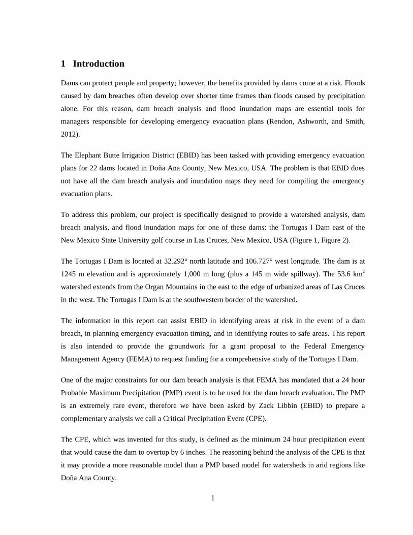
Dams can protect people and property; however, the benefits provided by dams come at a risk. Floods
caused by dam breaches often develop over shorter time frames than floods caused by precipitation
alone. For this reason, dam breach analysis and flood inundation maps are essential tools for
managers responsible for developing emergency evacuation plans (Rendon, Ashworth, and Smith,
2012).
The Elephant Butte Irrigation District (EBID) has been tasked with providing emergency evacuation
plans for 22 dams located in Doña Ana County, New Mexico, USA. The problem is that EBID does
not have all the dam breach analysis and inundation maps they need for compiling the emergency
evacuation plans.
To address this problem, our project is specifically designed to provide a watershed analysis, dam
breach analysis, and flood inundation maps for one of these dams: the Tortugas I Dam east of the
New Mexico State University golf course in Las Cruces, New Mexico, USA (Figure 1, Figure 2).
The Tortugas I Dam is located at 32.292° north latitude and 106.727° west longitude. The dam is at
1245 m elevation and is approximately 1,000 m long (plus a 145 m wide spillway). The 53.6 km2
watershed extends from the Organ Mountains in the east to the edge of urbanized areas of Las Cruces
in the west. The Tortugas I Dam is at the southwestern border of the watershed.
The information in this report can assist EBID in identifying areas at risk in the event of a dam
breach, in planning emergency evacuation timing, and in identifying routes to safe areas. This report
is also intended to provide the groundwork for a grant proposal to the Federal Emergency
Management Agency (FEMA) to request funding for a comprehensive study of the Tortugas I Dam.
One of the major constraints for our dam breach analysis is that FEMA has mandated that a 24 hour
Probable Maximum Precipitation (PMP) event is to be used for the dam breach evaluation. The PMP
is an extremely rare event, therefore we have been asked by Zack Libbin (EBID) to prepare a
complementary analysis we call a Critical Precipitation Event (CPE).
The CPE, which was invented for this study, is defined as the minimum 24 hour precipitation event
that would cause the dam to overtop by 6 inches. The reasoning behind the analysis of the CPE is that
it may provide a more reasonable model than a PMP based model for watersheds in arid regions like
Doña Ana County.

2
Figure 1. Tortugas Watershed, Las Cruces, NM, USA.
Figure 2. Close-up of Tortugas I Dam and surroundings.
3
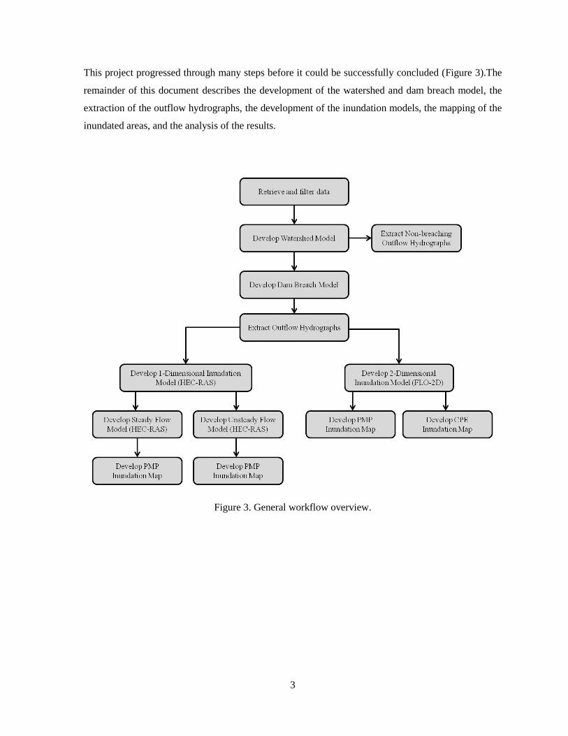
This project progressed through many steps before it could be successfully concluded (Figure 3).The
remainder of this document describes the development of the watershed and dam breach model, the
extraction of the outflow hydrographs, the development of the inundation models, the mapping of the
inundated areas, and the analysis of the results.
Figure 3. General workflow overview.
4
2 Methodology
There are three main parts to this project: 1) the watershed analysis, 2) the dam breach analysis, and
3) the inundation analysis. Each of these parts has its own series of questions that need to be
addressed and data to be collected before an engineering solution can be realized. The following
sections detail the data and preparation for the analyses along with the assumptions behind the
methods used in this study.
2.1 Data
Several types of data were essential for performing the analyses including:
Digital Terrain Model (DTM) data
Light Detection and Ranging (LIDAR) data
Orthophotos
Soil data
Land cover data, and
Precipitation data
The DTM data were downloaded from the New Mexico Resource Geographic Information System
program website maintained by the University of New Mexico (RGIS, 2012). The DTM data
included six New Mexico Digital Terrain Model 7.5-minute Quadrangles (2007) 10M enhanced
DEMs. The quadrangles used were:
Organ Peak, 32106-C5
Tortugas Mountain, 32106-C6
Las Cruces, 32106-C7
Bishop Cap, 32106-B5
San Miguel, 32106-B6
Black Mesa, 32106-B7
The New Mexico Digital Terrain Model Enhanced DEMs were specifically intended to be used for
water modeling, floodplain analysis, and environmental studies (RGIS, 2012). The six DTMs were
mosaiced into a single DTM using GRASS Geographic Information Systems (GIS) software
(GRASS, 2012). The DTMs were primarily used for the watershed analysis and the inundation
analysis using the HEC-RAS model. One FLO-2D model (FLO-2D, 2012) was run using DTMs to
get a rough estimate of the inundation area.
LIDAR data and orthophotos from 2010 covering most of the inundation area were provided by the
Doña Ana County Flood Commission. The LIDAR data were comprised of filtered bare earth points
showing the ground elevation. The orthophotos were received in .ecw format with a one foot
5
resolution. The orthophoto projection is New Mexico State Plane, Central Zone (FIPS 3002), U.S.
Feet with horizontal datum NAD 83 HARN and Vertical datum NAVD 88.
Soil data were extracted from maps provided by the Natural Resource Conservation Service (NRCS)
soil survey (NRCS, 2012). Land cover data were extracted from Environmental Protection Agency
2006 National Land Cover Data maps (EPA, 2012; Fry et al., 2011). Precipitation data and reference
materials were obtained from the National Oceanic and Atmospheric Administration, National
Weather Service Hydrometeorological Design Studies Center (NOAA, 2012).
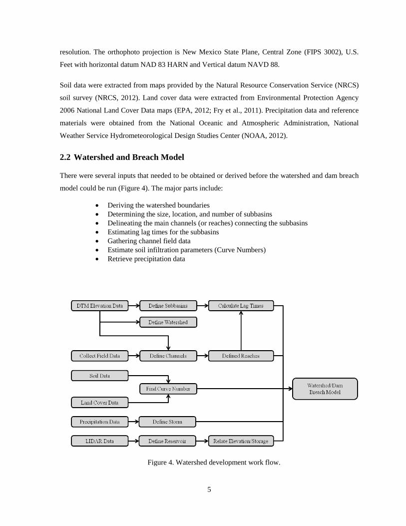
2.2 Watershed and Breach Model
There were several inputs that needed to be obtained or derived before the watershed and dam breach
model could be run (Figure 4). The major parts include:
Deriving the watershed boundaries
Determining the size, location, and number of subbasins
Delineating the main channels (or reaches) connecting the subbasins
Estimating lag times for the subbasins
Gathering channel field data
Estimate soil infiltration parameters (Curve Numbers)
Retrieve precipitation data
Figure 4. Watershed development work flow.
6
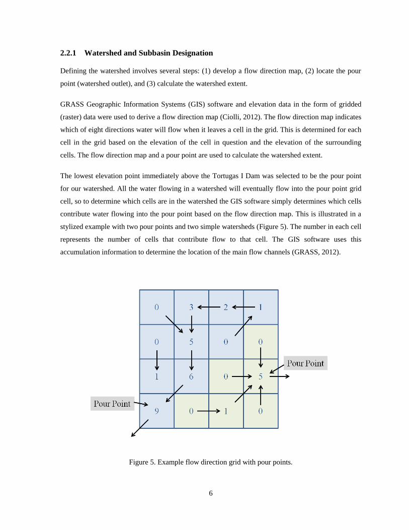
2.2.1 Watershed and Subbasin Designation
Defining the watershed involves several steps: (1) develop a flow direction map, (2) locate the pour
point (watershed outlet), and (3) calculate the watershed extent.
GRASS Geographic Information Systems (GIS) software and elevation data in the form of gridded
(raster) data were used to derive a flow direction map (Ciolli, 2012). The flow direction map indicates
which of eight directions water will flow when it leaves a cell in the grid. This is determined for each
cell in the grid based on the elevation of the cell in question and the elevation of the surrounding
cells. The flow direction map and a pour point are used to calculate the watershed extent.
The lowest elevation point immediately above the Tortugas I Dam was selected to be the pour point
for our watershed. All the water flowing in a watershed will eventually flow into the pour point grid
cell, so to determine which cells are in the watershed the GIS software simply determines which cells
contribute water flowing into the pour point based on the flow direction map. This is illustrated in a
stylized example with two pour points and two simple watersheds (Figure 5). The number in each cell
represents the number of cells that contribute flow to that cell. The GIS software uses this
accumulation information to determine the location of the main flow channels (GRASS, 2012).
Figure 5. Example flow direction grid with pour points.
7
We used GRASS GIS software (GRASS 2012) for the watershed analysis because the ESRI®
ArcGIS hydrology tools could not calculate the flow direction correctly (ArcGIS sometimes fails in
flat areas or areas with very low slope). GRASS GIS uses an AT least-cost search algorithm to
overcome this difficulty (GRASS, 2011).
The target number of subbasins for this study was 25. We determined that this would provide enough
subbasins to reflect the diversity of the watershed without creating data management problems (due to
having too many subbasins with corresponding parameters). We attempted to select basins that
reflected the changes in soil type, land cover, and slope variation. This was not always possible as the
water flow boundaries and the other subbasin characteristics did not always align.
We compromised by selecting subbasins that balanced the flow length and changes in slope: this
required compensating for overlapping soil classes by using a weighted average (described later in
this document). Our final decision was to use 28 subbasins instead of 25 because some of the
subbasins were too long and narrow and needed to be divided (Appendix, Table 6).
2.2.2 Channel Extraction and Reach Definition
We used GRASS GIS to compute the accumulated number of cells that contribute water to each cell
in the grid. Grids cells with high accumulations of water (from other upstream cells) were designated
as channels. We only used stream sections that connected the pour points of upstream subbasins with
the pour points of downstream subbasins. GIS tools were used to measure the length and elevation
change of the channels connecting the subbasins (Appendix, Table 7).
We physically visited several channels in the watershed to get representative data about the
vegetation density and to measure the width and side slopes of the selected channels. We inspected 12
channels that we thought would be representative for the majority of the channels in the watershed.
We also use Google Earth to estimate some of the channel characteristic for channels we could not
reach physically (due to restricted access) or that could not be assessed from the ground (due to
channel complexity or because the channels were too extensive to view from the ground).
Google Earth (Google, 2009) was particularly useful for the lower reaches of the watershed where
construction and irregular shapes of the channels made the channels hard to identify from ground
level. For the watershed model we used cross section data extracted from DTMs and modified the
cross sections into simple trapezoidal shapes based on our field data (Figure 6).
8
Figure 6. Example Excel™ profile used as a guide to define the cross sections in HEC-RAS.
2.2.3 Calculating Lag Times
Once the subbasins and channels were defined, we needed to calculate the lag time associated with
each subbasin (Appendix, Table 8). Lag times for the subbasins were estimated by multiplying 0.6
times the Kirpich Equation (Chin, 2006) described as:
(1)
where is the lag time, L is the flow length, and So is the average slope along the flow path. We used
the Kirpich equation because it is easy to understand and implement and it is one of the methods
commonly used (Chin, 2006).
When the flow path used for calculating the lag time traversed large changes in slope, the path was
divided into subsections. This was mainly necessary for the basins at the highest elevations, where the
path left the valley channels and followed smaller channels towards the ridges and peaks in the Organ
Mountains. The lengths of the paths were measured using GIS tools. The longest path was estimated
by first following the subbasins main channel (or reach) from the pour point to near the top of the
subbasin, then visually continuing the flow path overland towards the most distant part of the
subbasin upstream of the channel.
9
2.2.4 Reach Cross Section Sensitivity Analysis using HEC-RAS
In an effort to fine tune the watershed model, elevation data were extracted from the DTM mosaic to
create a reach cross-sections in HEC-RAS. A contour map with 2 m contour intervals was created in
GRASS GIS and layered over the DTM to help visualize the reach. We selected a representative cross
section near the half way point of the reach. A GRASS GIS tool was used to extract the cross section
channel profile at the selected location. The extracted cross section was then used as input to a HEC-
RAS model to simulate the reach properties.
In HEC-RAS we defined a reach using the cross section profile. We then created a simple trapezoid
channel cross section which we added to a different part of the reach. We adjusted the trapezoid
dimensions until the friction losses per unit length of channel were similar for both cross sections
(Figure 7, and Appendix, Figure 37). The kinetic energy was not identical; however, this was only a
preliminary investigation so we ignored the difference.
(a)
(b)
Figure 7. (a) Extracted cross section, and (b) equivalent trapezoidal cross section, Reach 27.
10
We substituted the new trapezoidal cross section developed in HEC-RAS for the original cross
section in the HEC-HMS model and compared the results. The resulting change in flow for the tested
reach was less than 1 m3/s. Since the flow difference for the tested reach was so small, we decided to
abandon this extra procedure.
2.2.5 Curve Number Definition
Watershed runoff is not only determined by spatial characteristics; runoff is also influenced by the
soil properties. We began our analysis of the soil properties by downloading soil survey maps (Figure
8) for Doña Ana County from the Natural Resource Conservation Service (NRCS 2012). The most
important information we obtained from these maps was the soil hydrologic group (Table 1).
We also used national land cover maps to classify the watershed land cover (EPA, 2012). We
classified the majority of the watershed as desert shrub/scrub in poor condition with some isolated
areas in the Organ Mountains classified as woodland in poor condition.
The soil hydrologic group data and the land cover classification were combined to determine the
Curve Number (CN) from tables in the WinTR-55 Watershed Hydrology software (USDA, 2012).
Curve numbers are used as input in the HEC-HMS watershed modeling software. Since most of the
subbasins included more than one soil type (and thus more than one CN) we used an area weighted
average to calculate the representative CN for each subbasin.
Figure 8. Soil map with the subbasins outlined (not available for higher elevations).
11
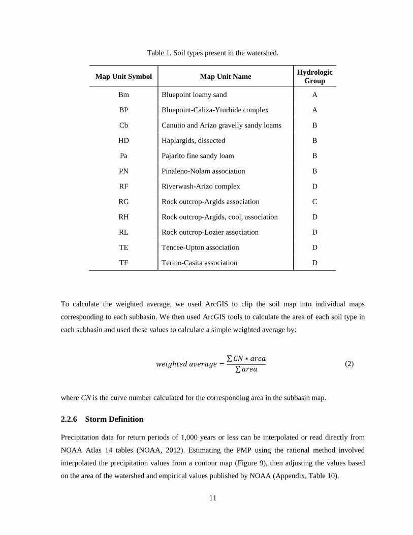
Table 1. Soil types present in the watershed.
Map Unit Symbol Map Unit Name Hydrologic
Group
Bm Bluepoint loamy sand A
BP Bluepoint-Caliza-Yturbide complex A
Cb Canutio and Arizo gravelly sandy loams B
HD Haplargids, dissected B
Pa Pajarito fine sandy loam B
PN Pinaleno-Nolam association B
RF Riverwash-Arizo complex D
RG Rock outcrop-Argids association C
RH Rock outcrop-Argids, cool, association D
RL Rock outcrop-Lozier association D
TE Tencee-Upton association D
TF Terino-Casita association D
To calculate the weighted average, we used ArcGIS to clip the soil map into individual maps
corresponding to each subbasin. We then used ArcGIS tools to calculate the area of each soil type in
each subbasin and used these values to calculate a simple weighted average by:
(2)
where CN is the curve number calculated for the corresponding area in the subbasin map.
2.2.6 Storm Definition
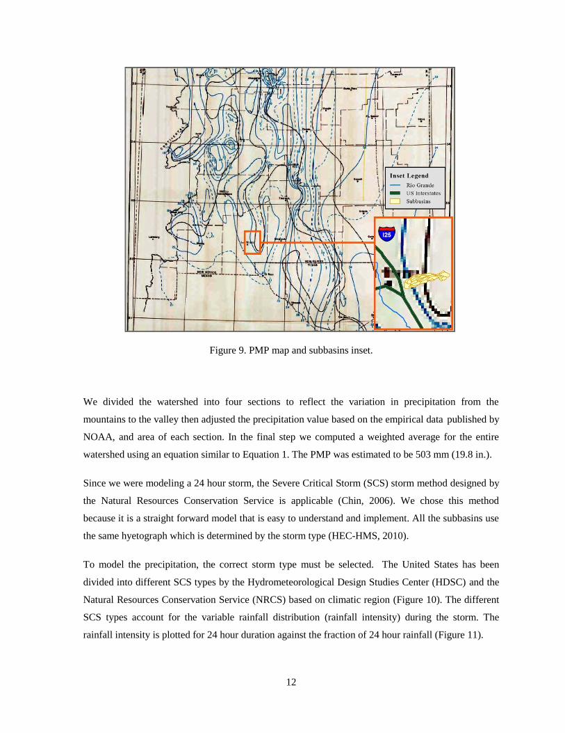
Precipitation data for return periods of 1,000 years or less can be interpolated or read directly from
NOAA Atlas 14 tables (NOAA, 2012). Estimating the PMP using the rational method involved
interpolated the precipitation values from a contour map (Figure 9), then adjusting the values based
on the area of the watershed and empirical values published by NOAA (Appendix, Table 10).
12
Figure 9. PMP map and subbasins inset.
We divided the watershed into four sections to reflect the variation in precipitation from the
mountains to the valley then adjusted the precipitation value based on the empirical data published by
NOAA, and area of each section. In the final step we computed a weighted average for the entire
watershed using an equation similar to Equation 1. The PMP was estimated to be 503 mm (19.8 in.).
Since we were modeling a 24 hour storm, the Severe Critical Storm (SCS) storm method designed by
the Natural Resources Conservation Service is applicable (Chin, 2006). We chose this method
because it is a straight forward model that is easy to understand and implement. All the subbasins use
the same hyetograph which is determined by the storm type (HEC-HMS, 2010).
To model the precipitation, the correct storm type must be selected. The United States has been
divided into different SCS types by the Hydrometeorological Design Studies Center (HDSC) and the
Natural Resources Conservation Service (NRCS) based on climatic region (Figure 10). The different
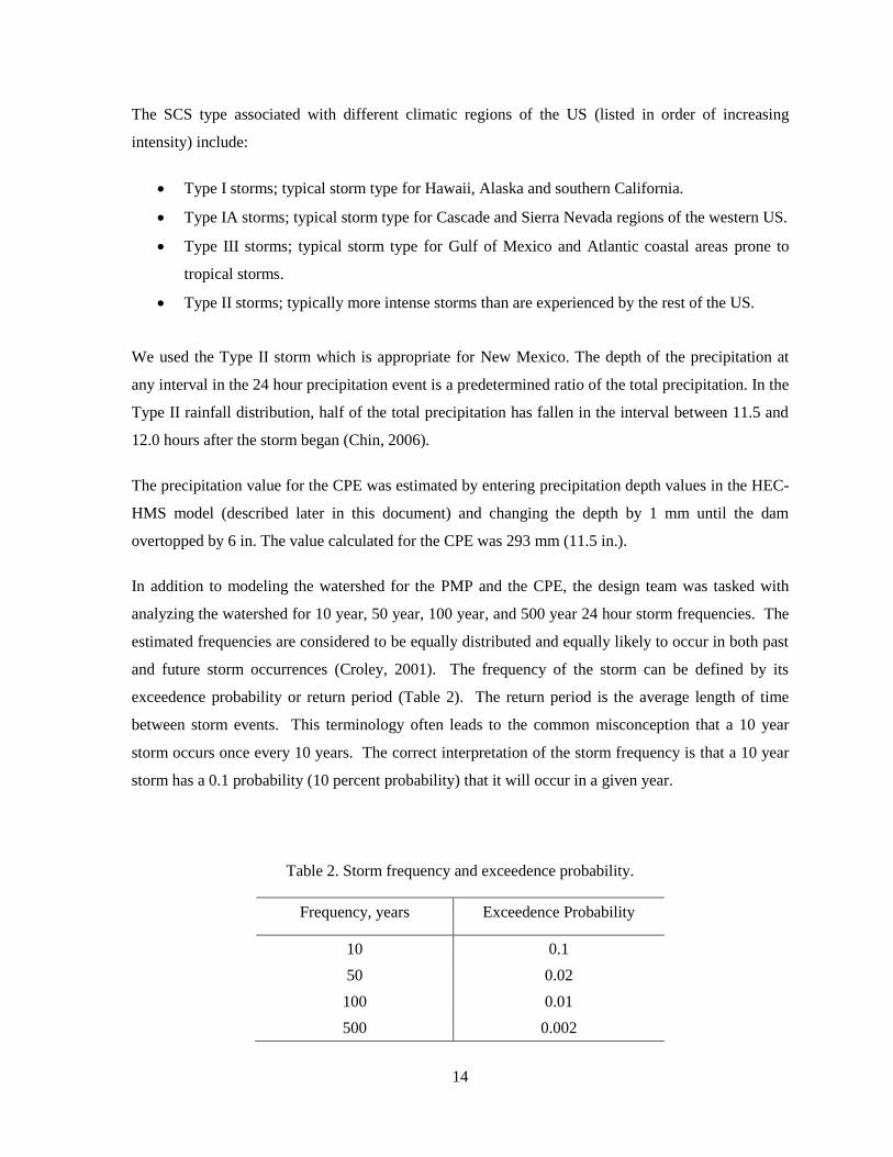
SCS types account for the variable rainfall distribution (rainfall intensity) during the storm. The
rainfall intensity is plotted for 24 hour duration against the fraction of 24 hour rainfall (Figure 11).
13
Figure 10. SCS Types for the United States (U.S. Type Storms map, 2012).
Figure 11. Standard SCS Type rainfall distribution
(Rainfall Distribution Curve, 2012).
14
The SCS type associated with different climatic regions of the US (listed in order of increasing
intensity) include:
Type I storms; typical storm type for Hawaii, Alaska and southern California.
Type IA storms; typical storm type for Cascade and Sierra Nevada regions of the western US.
Type III storms; typical storm type for Gulf of Mexico and Atlantic coastal areas prone to
tropical storms.
Type II storms; typically more intense storms than are experienced by the rest of the US.
We used the Type II storm which is appropriate for New Mexico. The depth of the precipitation at
any interval in the 24 hour precipitation event is a predetermined ratio of the total precipitation. In the
Type II rainfall distribution, half of the total precipitation has fallen in the interval between 11.5 and
12.0 hours after the storm began (Chin, 2006).
The precipitation value for the CPE was estimated by entering precipitation depth values in the HEC-
HMS model (described later in this document) and changing the depth by 1 mm until the dam
overtopped by 6 in. The value calculated for the CPE was 293 mm (11.5 in.).
In addition to modeling the watershed for the PMP and the CPE, the design team was tasked with
analyzing the watershed for 10 year, 50 year, 100 year, and 500 year 24 hour storm frequencies. The
estimated frequencies are considered to be equally distributed and equally likely to occur in both past
and future storm occurrences (Croley, 2001). The frequency of the storm can be defined by its
exceedence probability or return period (Table 2). The return period is the average length of time
between storm events. This terminology often leads to the common misconception that a 10 year
storm occurs once every 10 years. The correct interpretation of the storm frequency is that a 10 year
storm has a 0.1 probability (10 percent probability) that it will occur in a given year.
Table 2. Storm frequency and exceedence probability.
Frequency, years Exceedence Probability
10 0.1
50 0.02
100 0.01
500 0.002
15
2.2.7 Reservoir Elevation/Storage Relationship
Before the dam breach analysis could be started, a relationship between the volume of water and the
elevation of the water stored by the dam needed to be established. In this study LIDAR data were first
converted to elevation data (DTMs), then GIS tools were used to convert calculate the reservoir
volumes based on the elevation and spatial data represented by the DTMs.
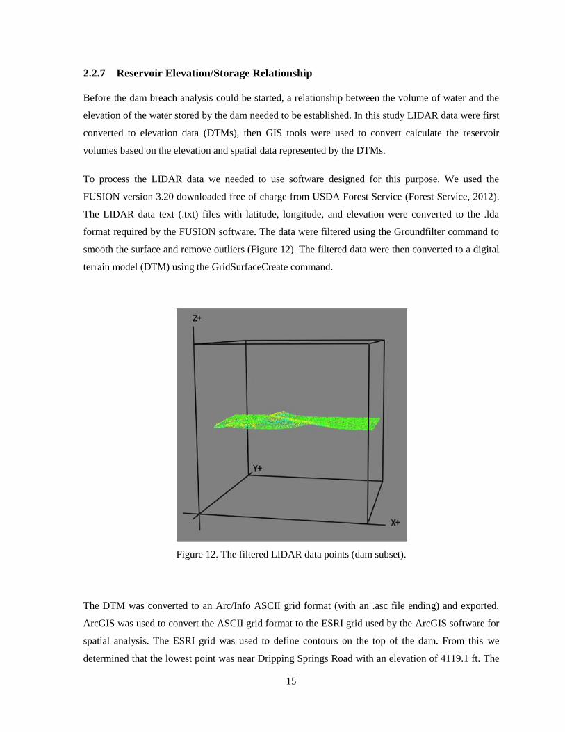
To process the LIDAR data we needed to use software designed for this purpose. We used the
FUSION version 3.20 downloaded free of charge from USDA Forest Service (Forest Service, 2012).
The LIDAR data text (.txt) files with latitude, longitude, and elevation were converted to the .lda
format required by the FUSION software. The data were filtered using the Groundfilter command to
smooth the surface and remove outliers (Figure 12). The filtered data were then converted to a digital
terrain model (DTM) using the GridSurfaceCreate command.
Figure 12. The filtered LIDAR data points (dam subset).
The DTM was converted to an Arc/Info ASCII grid format (with an .asc file ending) and exported.
ArcGIS was used to convert the ASCII grid format to the ESRI grid used by the ArcGIS software for
spatial analysis. The ESRI grid was used to define contours on the top of the dam. From this we
determined that the lowest point was near Dripping Springs Road with an elevation of 4119.1 ft. The
16
elevations we obtained using the LIDAR data were approximately 1.5 ft higher than the elevations
described in the old engineering documents we received from EBID. This could be the result of
undocumented changes in the dam construction; however, it is more likely that the differences are the
result of using different vertical datums. We concluded that the differences would be consistent for all
the reservoir volume calculations and therefore choose to overlook the difference. We later confirmed
that the volumes we calculated and the original engineering volume calculation were only 2.3%
different, so we were satisfied with this decision.
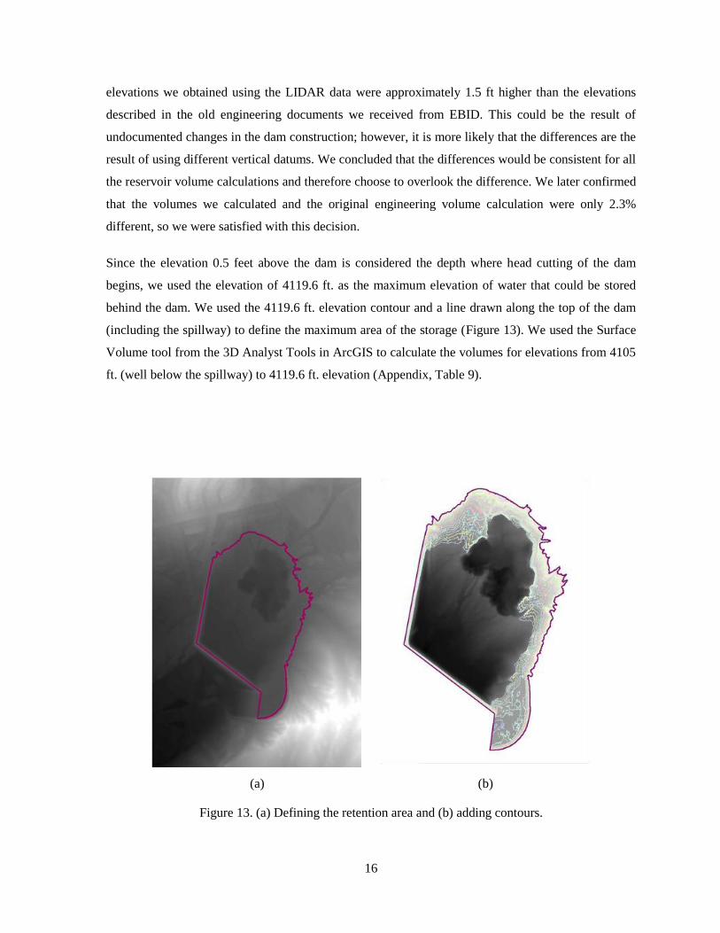
Since the elevation 0.5 feet above the dam is considered the depth where head cutting of the dam
begins, we used the elevation of 4119.6 ft. as the maximum elevation of water that could be stored
behind the dam. We used the 4119.6 ft. elevation contour and a line drawn along the top of the dam
(including the spillway) to define the maximum area of the storage (Figure 13). We used the Surface
Volume tool from the 3D Analyst Tools in ArcGIS to calculate the volumes for elevations from 4105
ft. (well below the spillway) to 4119.6 ft. elevation (Appendix, Table 9).
(a) (b)
Figure 13. (a) Defining the retention area and (b) adding contours.
17
2.2.8 Additional Watershed Parameters
Version 3.5 of the Hydrologic Modeling System HEC-HMS, developed by the Hydrologic
Engineering Center of the U.S. Army Corps of Engineers, was used to model the watershed (HEC-
HMS, 2010). This model can use the watershed physical properties and meteorological data to model
the accumulated runoff due to precipitation in a watershed. It also incorporates software that can use
dam physical properties to model a dam breach and the subsequent outflow hydrograph. The
hydrograph can be used in other software to model the inundation and produce inundation maps.
There are several addition decisions that must be made before running the HEC-HMS model:
Canopy method
Evapotranspiration
Surface method
Loss method
Transform method
Baseflow method
Impervious percent
Routing method
Loss/gain method
Manning’s roughness coefficient
Precipitation method
Time frame
The vegetation in this watershed is sparse, therefore we considered the moisture intercepted by the
canopy to be negligible in relation to the total precipitation and set the canopy method to none. We
considered plant transpiration to be negligible as well. Evaporation from the soil surface could be
factor, particularly in the beginning of the storm; however, to simplify the model and implement the
worst case scenario, evaporation was neglected as well.
The surface method accounts for water storage in depressions found in the watershed surface. We did
not have enough information to implement a surface method so it was neglected in this study. This is
something that could be investigated in a comprehensive study of the Tortugas I Dam.
The loss method accounts for infiltration losses that reduce runoff. For this study we used the SCS
Curve Number loss. This method calculates the amount of precipitation that infiltrates into the soil
profile based on the CN numbers for each time step in the model. We did not enter an initial
abstraction, so HEC-HMS added an abstraction equal to 0.2 times the potential retention calculated
from the CN (HEC-HMS, 2010).

18
We used the SCS Unit Hydrograph transform method because it is easy to use and understand. The
runoff is calculated using a unit hydrograph where the runoff at any point in the storm is calculated
using the ration of the time in question and the time to peak runoff. This ratio points to another ratio
between the runoff and the peak runoff (Chin, 2010). The HEC-HMS software calculates the time to
peak run-off and the peak runoff, so we only needed to provide the lag time for each subbasin
(Equation 1).
We set the baseflow to zero which is reasonable since the watershed is located in an arid region where
the valleys and arroyos are normally dry (unless there has been a recent precipitation event). The
watershed is also relatively undeveloped, so we considered the percent impervious surface (e.g.,
rooftops and parking lots) to be negligible and set this parameter to zero for all the subbasins.
We selected the Kinematic Wave routing method to model the flow in the reaches. The Kinematic
Wave method is best suited to steep streams, which are typical for this watershed. The number of
subreaches parameter was set to the length of the reach divided by 1,000 to reflect that some of the
reaches were quite long (Appendix, Table 7). The HEC-HMS program will automatically determine
the correct number of subreaches, so the subreaches parameter is treated as a suggestion and may be
overridden by HEC-HMS when the simulation is run (HEC-HMS, 2010).
Because of a lack of data, we set the Loss/Gain method for the reaches to none. The loss of runoff to
infiltration may be negligible; however, this should be addressed in future investigations.
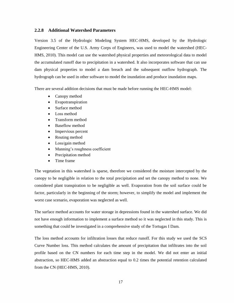
The Manning’s roughness coefficient we selected for the reaches varied according to location (Figure
14). The majority of the reaches had scattered brush and weeds so we used a Manning’s roughness
coefficient of 0.030. In areas we judged to have denser growth we increased this to 0.035. Some mid
elevation areas were mostly sparse grass and weeds, so we used a coefficient of 0.025.
A small set of reaches in the higher elevations had very dense trees and shrubs with large boulders,
and we assumed the flow would reach the lower branches of the trees. For these reaches we used a
coefficient of 0.12. We did not consider whether a PMP storm would uproot all the vegetation and
develop a scoured reach with a reduced Manning’s coefficient.
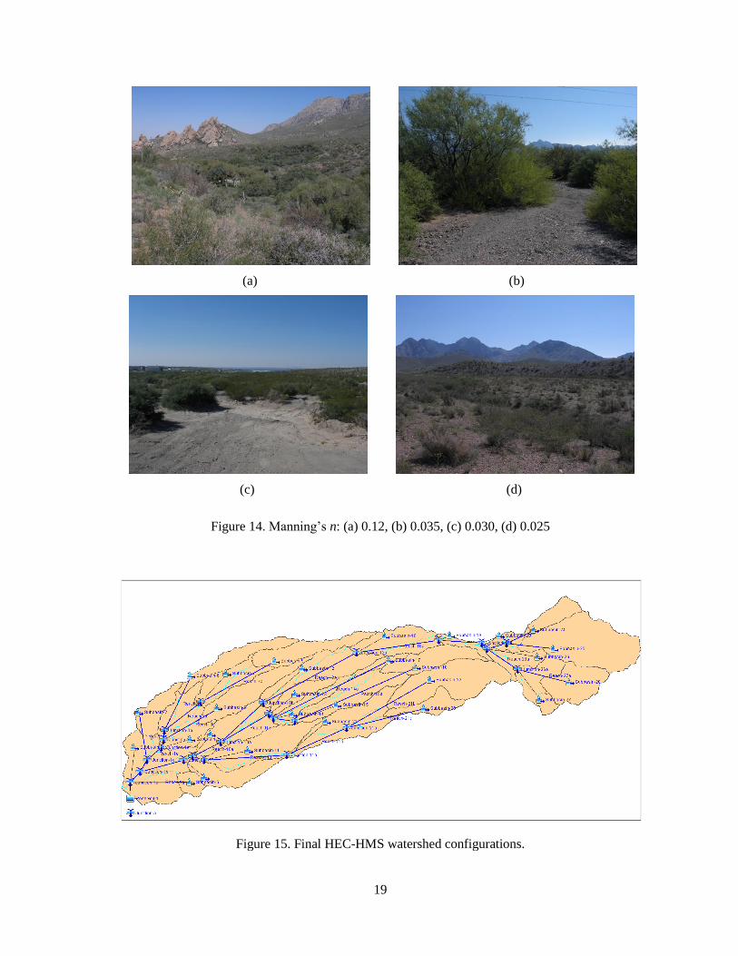
To ensure the model would run to completion we set the model time to three days. Since the lag time
for some of the basins was very short we set the time interval to two minutes, which is less than one
third of the shortest lag time (Appendix, Table 8). The final watershed model had 28 subbasins and 27
reaches (Figure 15). After the watershed model was completed we added the dam breach parameters.
19
(a) (b)
(c) (d)
Figure 14. Manning’s n: (a) 0.12, (b) 0.035, (c) 0.030, (d) 0.025
Figure 15. Final HEC-HMS watershed configurations.
20
2.2.9 Dam Breach Parameters
To model the dam breach, a reservoir component was added to the HEC-HMS model (Table 3). We
selected the Elevation-Storage routing method for modeling the reservoir because we could use GIS
to calculate the elevation storage relationship for the reservoir. We set the initial conditions for the
reservoir to zero initial storage because the reservoir is normally empty. We added the Outflow
Structures method to account for the spillway flow prior to dam breach.
The outflow assumptions that we used were: (1) the water level in the reservoir is level, (2) the
spillway flow is a function of the reservoir elevation, and (3) the outlet pipe under the dam is not
functioning. We selected the Broad-Crested Spillway method and set the coefficient to 2.6 to account
for energy losses as the water enters the spillway. Typical values range from 2.6 to 4.0, so we selected
the lower end to maximize flow over the spillway before the dam breach (HEC-HMS, 2010). This
parameter should be checked in follow-up investigations to see whether this assumption is valid.
For the dam breach, we selected the elevations trigger method based on the assumption that the dam
would fail because of overtopping and face head erosion (HEC-HMS, 2010). We also assumed that
the water elevation in the reservoir would still be increasing rapidly (and the breach would occur
quickly) so we set the development time to 0.125 hours (8 minutes).
The lowest part of the dam is directly east of Dripping Springs Road. Immediately after the breach
begins, water could flow directly down the road; however, since we assume the dam will breach
quickly, the majority of the water should soon be flowing down the valley through the golf course.
We assumed that the dam breach would assume a roughly trapezoidal shape with the dimensions
approximately the same as the shape above the dam as determined from the LIDAR based contour
maps (Table 3). The lowest area just above the dam was a roughly level stretch 450 m wide. The
south slope is steeper than the north slope because of the concrete spillway.
Our assumptions may be excessive and future work related to the Tortugas I Dam should investigate
this aspect of the model design more thoroughly. Another aspect we did not consider is whether the
dam breach would remove the spillway.
21
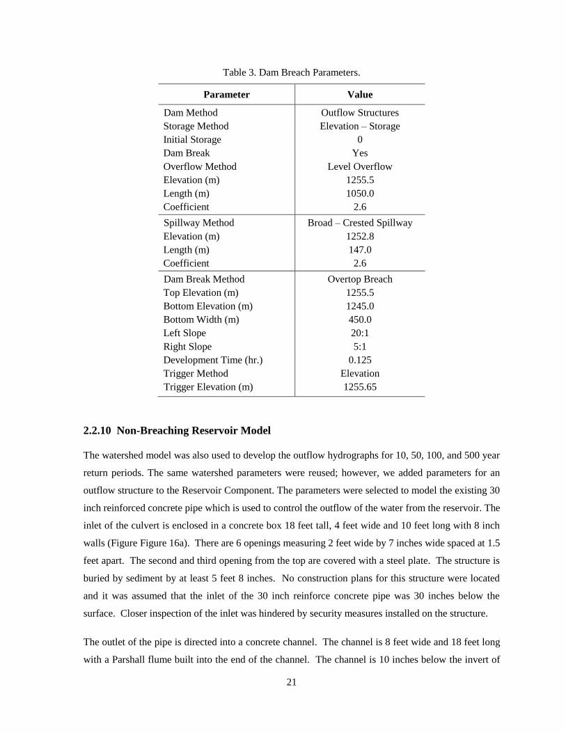
Table 3. Dam Breach Parameters.
Parameter Value
Dam Method Outflow Structures
Storage Method Elevation – Storage
Initial Storage 0
Dam Break Yes
Overflow Method Level Overflow
Elevation (m) 1255.5
Length (m) 1050.0
Coefficient 2.6
Spillway Method Broad – Crested Spillway
Elevation (m) 1252.8
Length (m) 147.0
Coefficient 2.6
Dam Break Method Overtop Breach
Top Elevation (m) 1255.5
Bottom Elevation (m) 1245.0
Bottom Width (m) 450.0
Left Slope 20:1
Right Slope 5:1
Development Time (hr.) 0.125
Trigger Method Elevation
Trigger Elevation (m) 1255.65
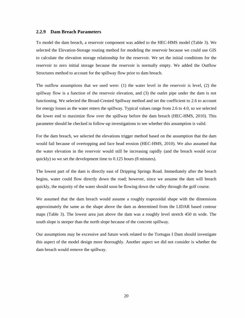
2.2.10 Non-Breaching Reservoir Model
The watershed model was also used to develop the outflow hydrographs for 10, 50, 100, and 500 year
return periods. The same watershed parameters were reused; however, we added parameters for an
outflow structure to the Reservoir Component. The parameters were selected to model the existing 30
inch reinforced concrete pipe which is used to control the outflow of the water from the reservoir. The
inlet of the culvert is enclosed in a concrete box 18 feet tall, 4 feet wide and 10 feet long with 8 inch
walls (Figure Figure 16a). There are 6 openings measuring 2 feet wide by 7 inches wide spaced at 1.5
feet apart. The second and third opening from the top are covered with a steel plate. The structure is
buried by sediment by at least 5 feet 8 inches. No construction plans for this structure were located
and it was assumed that the inlet of the 30 inch reinforce concrete pipe was 30 inches below the
surface. Closer inspection of the inlet was hindered by security measures installed on the structure.
The outlet of the pipe is directed into a concrete channel. The channel is 8 feet wide and 18 feet long
with a Parshall flume built into the end of the channel. The channel is 10 inches below the invert of
22
the pipe and the invert of the pipe is 35 inches above ground elevation (Figure 16b). The inlet and
outlet elevations were determined using ArcGIS and the DTM for the Tortugas I Dam. The invert
elevation was then subtracted from the surface elevations.
(a) (b)
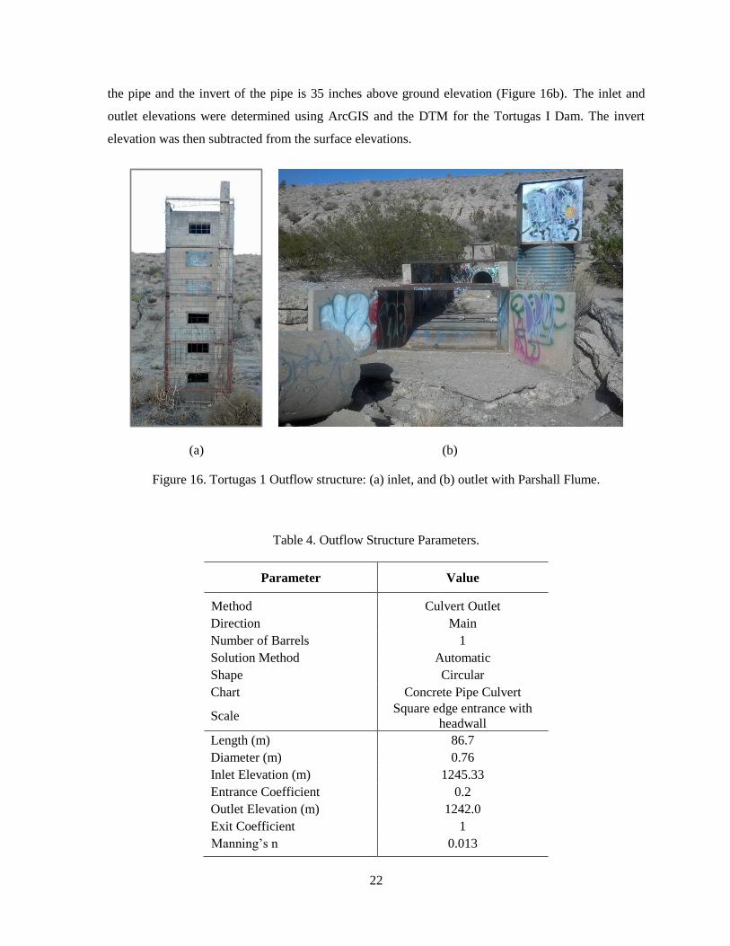
Figure 16. Tortugas 1 Outflow structure: (a) inlet, and (b) outlet with Parshall Flume.
Table 4. Outflow Structure Parameters.
Parameter Value
Method Culvert Outlet
Direction Main
Number of Barrels 1
Solution Method Automatic
Shape Circular
Chart Concrete Pipe Culvert
Scale Square edge entrance with
headwall
Length (m) 86.7
Diameter (m) 0.76
Inlet Elevation (m) 1245.33
Entrance Coefficient 0.2
Outlet Elevation (m) 1242.0
Exit Coefficient 1
Manning’s n 0.013
23
The precipitations data were added to HEC-HMS by using the Meteorologic Model Manager.
Separate meteorologic models were created for the 10, 50, 100, and 500 years return periods. Several
parameters were entered:
The precipitation parameter was set to “SCS Storm”
Evapotranspiration was set to “None” under the same logic that evaporation will occur at the
onset of the storm but to obtain worst case scenario, it should be ignored
Snowmelt parameter was set to “None” since the area rarely encounters significant amounts
of snow pack that will result in runoff
Unit System set to “Metric”
The Method was set to “Type 2”
The precipitation depth was set to the value corresponded to the return period for a 24 hour
storm period obtained from the HDSC Precipitation Frequency Data Server website
(Appendix, Figure 38).
After the setting up the meteorologic models, simulations were performed for each storm frequency.
The simulations painted a picture of what can be expected based on the parameters and assumptions
made in the creation of the model. These simulations should be rerun when additional data are
acquired.
2.3 Inundation Models
2.3.1 FLO-2D Model
FLO-2D is a two dimensional flood routing model that uses a finite difference model and volume
conservation to route unconfined surface water flow over complex topography. We used FLO-2D
Version 2009.06 which is on FEMA’s list of approved hydraulic models for riverine and unconfined
alluvial fan flood studies. Newer versions of FLO-2D are available.
The LIDAR data and the flow hydrographs generated by the watershed models were the only inputs
used for the FLO-2D models described in this report. Future work should include: (1) channels
representing the accelerated flow along major roads, (2) cross sections representing the constrictions
of flow caused by Interstates I-10 and I-25, and (3) localized data on Manning’s roughness
coefficient. It may also be interesting to include larger structures in the inundated areas (e.g., large
building on the NMSU campus) to see if they deflect the modeled flow.

24
The FLO-2D model was based on the LIDAR data and the watershed outflow hydrographs. The
LIDAR data were separated into 31 files, so we could not open a new FLO-2D project using them
directly. To overcome this problem we created a simple polygon outlining the extent of the combined
LIDAR data in ArcGIS and used the polygon as the basis for a new simulation project.
The polygon was also used as a guide to create a project grid and define the computation area for the
simulation. The LIDAR data could then be used to populate the grid with elevation information. FLO-
2D extracted and averaged the point data from the LIDAR files for each cell within the computation
area of the grid. One thing that may introduce error is that areas with roads may be missing LIDAR
data points so the road surfaces will not contribute to the average elevation for the related grid cells.
We decided to use 200 foot square grid cells for the simulation as this configuration would produce
simulation results in less than an hour using a 10 minute time step (the 150 foot square grid took so
long we canceled the simulation to try a larger grid). We also filtered the outflow hydrographs to 10
minute intervals from the original 2 minute intervals to speed up the processing. We reasoned that
since the hydrograph represents flow rates and not total flow quantities, the results of the simulation
would be similar for both time steps. Models were run for both the PMP and CPE.
Given the opportunity, the models should be re-run using (1) cross sections to represent major flow
constrictions such as those caused by the interstate highways, (2) adding channels following the major
roads to simulate the accelerated flow of water along these paths, and (3) modifying the Manning’s
roughness coefficients to model changes in the flow characteristics from urban to rural areas. Future
analysis should also consider manually adding elevation adjustments to model the flow deflection
caused by major structures (e.g., the Pan American Center, the Football Stadium).
2.3.2 HEC-RAS Model
HEC-RAS is a one-dimensional model designed to model stream flow. For this project we wanted to
compare the HEC-RAS inundations results with the FLO-2D results. We were specifically interested
in how well each model represented the likely inundation conditions as well as how difficult each
model was to implement. HEC-RAS was used to model the extent of the flooding and impact of dam
break parameters on the downstream water surface elevation. Some of the data were processed using
HEC-Geo-RAS (Meyer and Olivera, 2012) which is a flood plain analysis add-on module for ArcGIS
that is specifically designed to complement HEC-RAS. ArcGIS was also used to create the inundation
maps following the model runs.
25
HEC-RAS can be used to model both steady and unsteady flow conditions. The process for modeling
steady flow involved the following steps:
• Create RAS (Geospatial) Layers in ArcGIS for the flood stream
• Export the GIS Data to HEC-RAS
• Create the river hydraulics model in HEC-RAS
• Simulate the flood using the peak flow from the outflow hydrograph
• Complete the hydraulic Analysis in HEC-RAS
• Export the HEC-RAS data to ArcGIS
• Create the inundation map using ArcGIS
The process was repeated using the entire outflow hydrograph to simulate unsteady flow conditions.
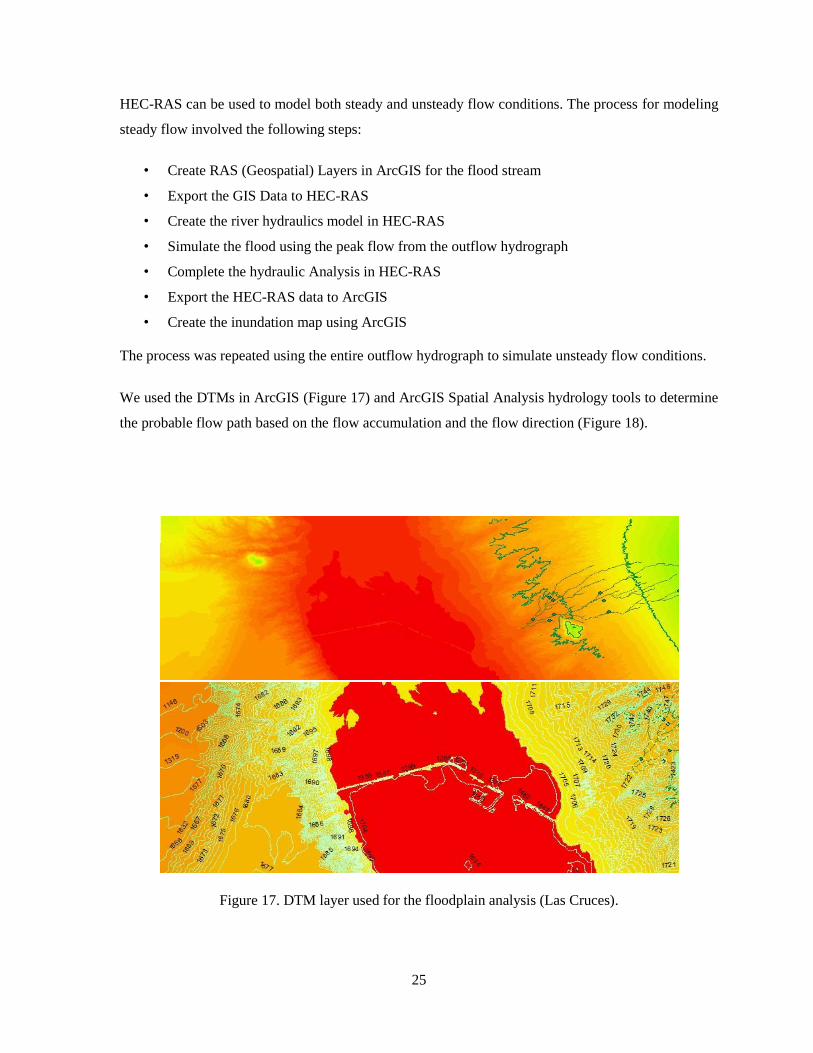
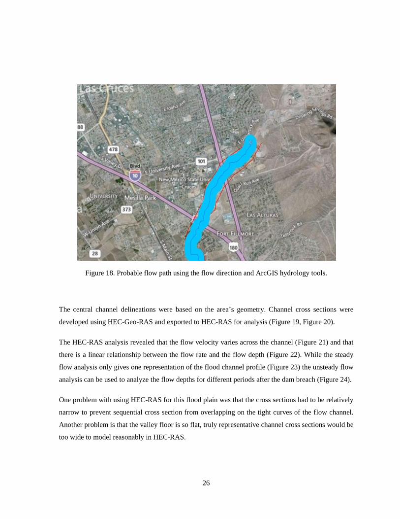
We used the DTMs in ArcGIS (Figure 17) and ArcGIS Spatial Analysis hydrology tools to determine
the probable flow path based on the flow accumulation and the flow direction (Figure 18).
Figure 17. DTM layer used for the floodplain analysis (Las Cruces).
26
Figure 18. Probable flow path using the flow direction and ArcGIS hydrology tools.
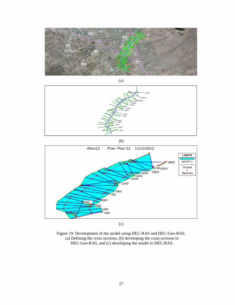
The central channel delineations were based on the area’s geometry. Channel cross sections were
developed using HEC-Geo-RAS and exported to HEC-RAS for analysis (Figure 19, Figure 20).
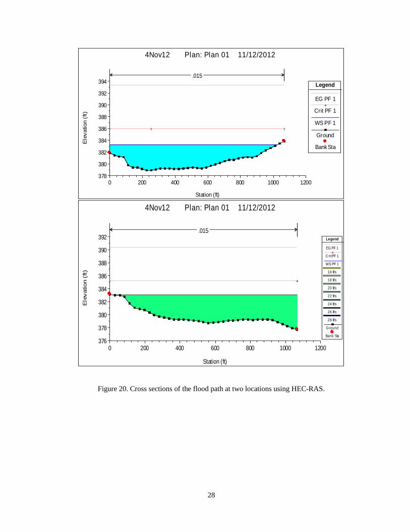
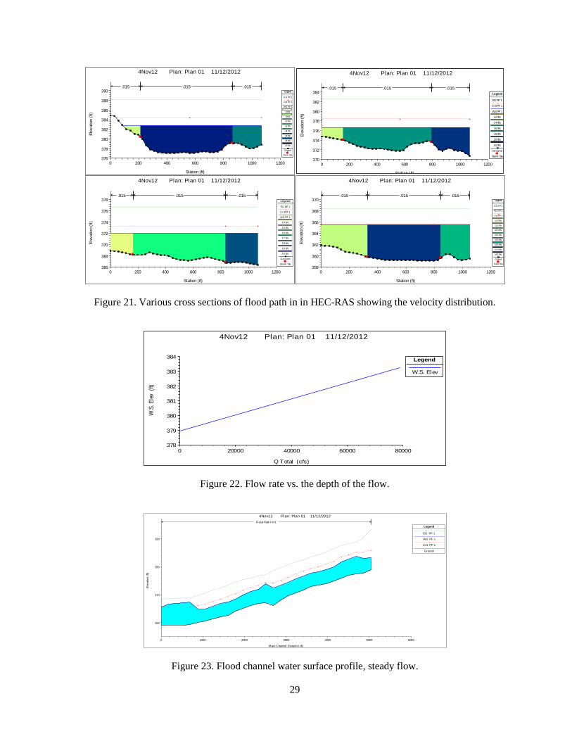
The HEC-RAS analysis revealed that the flow velocity varies across the channel (Figure 21) and that
there is a linear relationship between the flow rate and the flow depth (Figure 22). While the steady
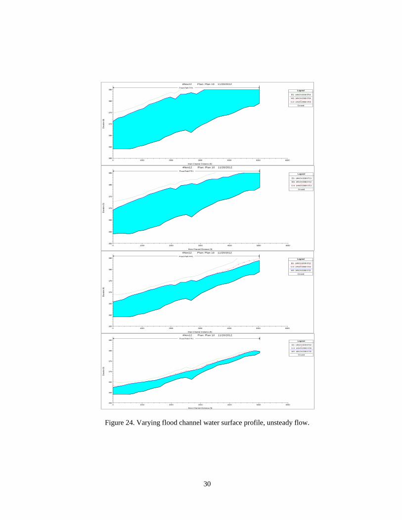
flow analysis only gives one representation of the flood channel profile (Figure 23) the unsteady flow
analysis can be used to analyze the flow depths for different periods after the dam breach (Figure 24).
One problem with using HEC-RAS for this flood plain was that the cross sections had to be relatively
narrow to prevent sequential cross section from overlapping on the tight curves of the flow channel.
Another problem is that the valley floor is so flat, truly representative channel cross sections would be
too wide to model reasonably in HEC-RAS.
27
(a)
(b)
(c)
Figure 19. Development of the model using HEC-RAS and HEC-Geo-RAS.
(a) Defining the cross sections, (b) developing the cross sections in
HEC-Geo-RAS, and (c) developing the model in HEC-RAS.
FR1
17400
16800
16200
15600
14400
13200
12600
11400
9600
9000
8400
7800
6600
5400
4800
2400
1800
1200
Flood Path
17400
16800
16200
15600
14400 13200
12600
11400
8400 7200
6600
4800
2400
1800
1200
4Nov12 Plan: Plan 01 11/12/2012
Legend
WS PF 1
Ground
Bank Sta
28
Figure 20. Cross sections of the flood path at two locations using HEC-RAS.
0 200 400 600 800 1000 1200378
380
382
384
386
388
390
392
394
4Nov12 Plan: Plan 01 11/12/2012
Station (ft)
Ele
vation (
ft)
Legend
EG PF 1
Crit PF 1
WS PF 1
Ground
Bank Sta
.015
0 200 400 600 800 1000 1200376
378
380
382
384
386
388
390
392
4Nov12 Plan: Plan 01 11/12/2012
Station (ft)
Ele
vation (
ft)
Legend
EG PF 1
C rit PF 1
WS PF 1
16 ft/s
18 ft/s
20 ft/s
22 ft/s
24 ft/s
26 ft/s
28 ft/s
Ground
Bank Sta
.015
29
Figure 21. Various cross sections of flood path in in HEC-RAS showing the velocity distribution.
Figure 22. Flow rate vs. the depth of the flow.
Figure 23. Flood channel water surface profile, steady flow.
0 200 400 600 800 1000 1200376
378
380
382
384
386
388
390
4Nov12 Plan: Plan 01 11/12/2012
Station (ft)
Ele
vatio
n (
ft)
Legend
EG PF 1
Crit PF 1
WS PF 1
6 ft/s
8 ft/s
10 ft/s
12 ft/s
14 ft/s
16 ft/s
18 ft/s
20 ft/s
Ground
Bank Sta
.015 .015 .015
0 200 400 600 800 1000 1200370
372
374
376
378
380
382
384
4Nov12 Plan: Plan 01 11/12/2012
Station (ft)
Ele
vatio
n (
ft)
Legend
EG PF 1
Crit PF 1
WS PF 1
12 ft/s
14 ft/s
16 ft/s
18 ft/s
20 ft/s
22 ft/s
Ground
Bank Sta
.015 .015 .015
0 200 400 600 800 1000 1200366
368
370
372
374
376
378
4Nov12 Plan: Plan 01 11/12/2012
Station (ft)
Ele
vatio
n (
ft)
Legend
EG PF 1
C rit PF 1
WS PF 1
14 ft/s
15 ft/s
16 ft/s
17 ft/s
18 ft/s
19 ft/s
20 ft/s
Ground
Bank Sta
.015 .015 .015
0 200 400 600 800 1000 1200358
360
362
364
366
368
370
4Nov12 Plan: Plan 01 11/12/2012
Station (ft)
Ele
vatio
n (
ft)
Legend
EG PF 1
WS PF 1
Crit PF 1
11.0 ft/s
11.5 ft/s
12.0 ft/s
12.5 ft/s
13.0 ft/s
13.5 ft/s
14.0 ft/s
14.5 ft/s
Ground
Bank Sta
.015 .015 .015
0 20000 40000 60000 80000378
379
380
381
382
383
384
4Nov12 Plan: Plan 01 11/12/2012
Q Total (cfs)
W.S
. Ele
v (
ft)
Legend
W.S. Elev
0 1000 2000 3000 4000 5000 6000
360
370
380
390
4Nov12 Plan: Plan 01 11/12/2012
Main Channel Distance (ft)
Ele
vatio
n (
ft)
Legend
EG PF 1
WS PF 1
Crit PF 1
Ground
Flood Path FR1
30
Figure 24. Varying flood channel water surface profile, unsteady flow.
0 1000 2000 3000 4000 5000 6000355
360
365
370
375
380
385
4Nov12 Plan: Plan 10 11/20/2012
Main Channel Distance (ft)
Ele
vatio
n (f
t)
Legend
EG 14NOV2008 0704
WS 14NOV2008 0704
Crit 14NOV2008 0704
Ground
Flood Path FR1
0 1000 2000 3000 4000 5000 6000355
360
365
370
375
380
385
4Nov12 Plan: Plan 10 11/20/2012
Main Channel Distance (ft)
Ele
vatio
n (
ft)
Legend
EG 14NOV2008 0713
WS 14NOV2008 0713
Crit 14NOV2008 0713
Ground
Flood Path FR1
0 1000 2000 3000 4000 5000 6000355
360
365
370
375
380
385
4Nov12 Plan: Plan 10 11/20/2012
Main Channel Distance (ft)
Ele
vatio
n (f
t)
Legend
EG 14NOV2008 0722
Crit 14NOV2008 0722
WS 14NOV2008 0722
Ground
Flood Path FR1
0 1000 2000 3000 4000 5000 6000355
360
365
370
375
380
385
4Nov12 Plan: Plan 10 11/20/2012
Main Channel Distance (ft)
Ele
vatio
n (f
t)
Legend
EG 14NOV2008 0730
Crit 14NOV2008 0730
WS 14NOV2008 0730
Ground
Flood Path FR1
31
3 Results and Discussion
This section reviews the results of the watershed, dam breach, and inundation analysis. The watershed
analysis results are primarily an inflow hydrograph for the reservoir, a dam storage curve, and a
spillway outflow hydrograph. The spill way outflow hydrograph shifts to a dam breach outflow
hydrograph after the dam breaks. The results of the inundation analysis include maps of the inundated
areas.
3.1 Watershed and Dam Breach
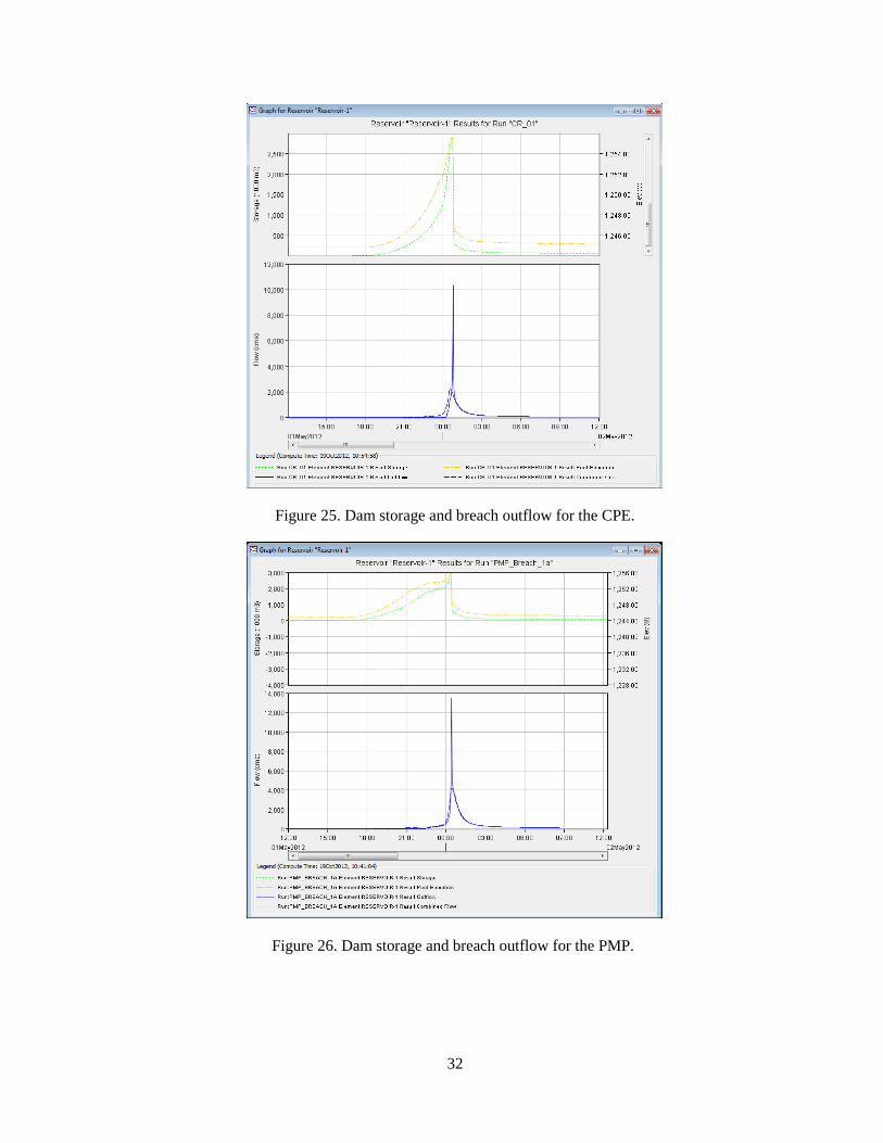
The CPE produced a peak flow of 2,240 m3/s into the reservoir with the peak occurring at 12 hours
and 32 minutes after the beginning of the storm. The total calculated inflow was 12.5∙106 m
3. The
peak outflow from the reservoir (after the dam breach) occurred at 12 hour and 46 minutes after the
storm began. The inflow and surge of stored water escaping the dam caused a spike with a peak
outflow of 10,300 m3/s. The total outflow was 12.2∙10
6 m
3 indicating that a small amount of water
was retained behind the broken dam. The peak storage of the reservoir was 2.89∙106 m
3 (Figure 25).
The PMP produced a peak flow of 4,200 m3/s into the reservoir with the peak occurring at 12 hours
and 28 minutes after the beginning of the storm. The total calculated inflow was 23.5∙106 m
3. The
peak outflow from the reservoir (after the dam breach) occurred at 12 hour and 26 minutes after the
storm began. The inflow and surge of stored water escaping the dam caused a spike with a peak
outflow of 13,500 m3/s. The total outflow was 23.2∙10
6 m
3 indicating that a small amount of water
was retained behind the broken dam. The peak storage of the reservoir was 2.95∙106 m
3 (Figure 26).
For the CPE the peak outflow occurred 14 minutes after the peak inflow. For the PMP the peak
outflow occurred two minutes before peak inflow. Although we expected large outflows from the
dam breach simulations, these coincident occurrences and the subsequent massive outflows were
unexpected. It must be remembered that part of the timing in these models is the result of the storm
method chosen.
Another thing worth noting is that the majority of the runoff occurs in a two hour time frame. This
indicates that the large flow volumes result in a rapid transport of the water from the highest
elevations to the outlet. According to the simulation results, the dam appears to have been over
designed. Notably, the CPE occurred at 293 mm (11.5 in.). This is nearly twice the precipitation depth
for a 24 hour storm with a 1,000 year return period (157 mm /6.2 in.) as published by NOAA Atlas 14
(NOAA, 2012) for the State University weather station.
32
Figure 25. Dam storage and breach outflow for the CPE.
Figure 26. Dam storage and breach outflow for the PMP.
33
3.2 Non-Breaching Outflow Hydrographs
This section presents the results of the 10, 50, 100, and 500 year 24 hour storm simulations.
3.2.1 The 10 Year 24 Hour Storm
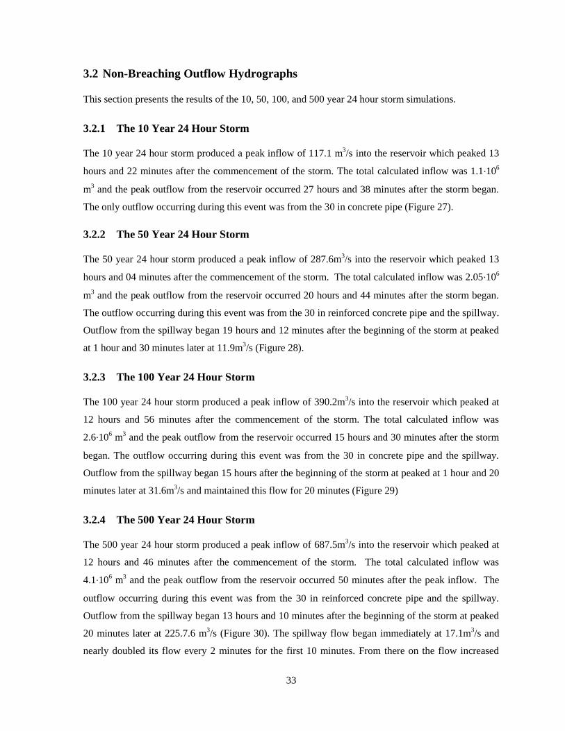
The 10 year 24 hour storm produced a peak inflow of 117.1 m3/s into the reservoir which peaked 13
hours and 22 minutes after the commencement of the storm. The total calculated inflow was 1.1·106
m3 and the peak outflow from the reservoir occurred 27 hours and 38 minutes after the storm began.
The only outflow occurring during this event was from the 30 in concrete pipe (Figure 27).
3.2.2 The 50 Year 24 Hour Storm
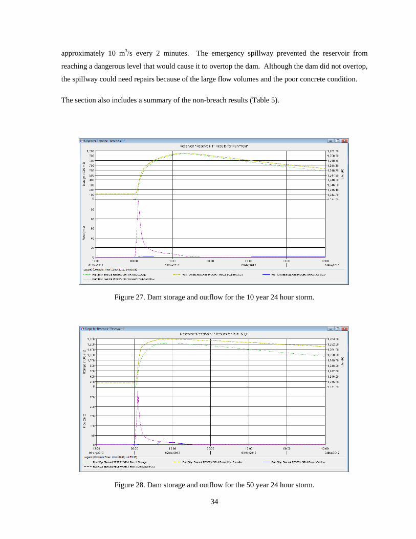
The 50 year 24 hour storm produced a peak inflow of 287.6m3/s into the reservoir which peaked 13
hours and 04 minutes after the commencement of the storm. The total calculated inflow was 2.05·106
m3 and the peak outflow from the reservoir occurred 20 hours and 44 minutes after the storm began.
The outflow occurring during this event was from the 30 in reinforced concrete pipe and the spillway.
Outflow from the spillway began 19 hours and 12 minutes after the beginning of the storm at peaked
at 1 hour and 30 minutes later at 11.9m3/s (Figure 28).
3.2.3 The 100 Year 24 Hour Storm
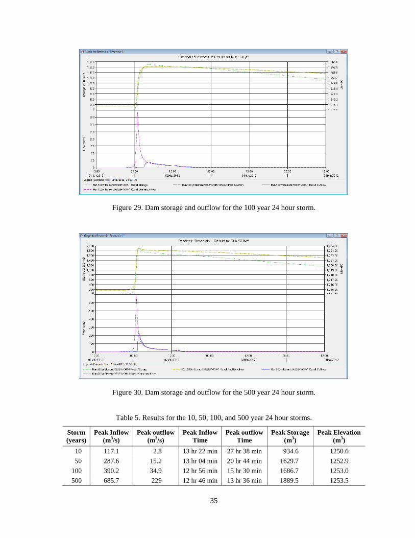
The 100 year 24 hour storm produced a peak inflow of 390.2m3/s into the reservoir which peaked at
12 hours and 56 minutes after the commencement of the storm. The total calculated inflow was
2.6·106 m
3 and the peak outflow from the reservoir occurred 15 hours and 30 minutes after the storm
began. The outflow occurring during this event was from the 30 in concrete pipe and the spillway.
Outflow from the spillway began 15 hours after the beginning of the storm at peaked at 1 hour and 20
minutes later at 31.6m3/s and maintained this flow for 20 minutes (Figure 29)
3.2.4 The 500 Year 24 Hour Storm
The 500 year 24 hour storm produced a peak inflow of 687.5m3/s into the reservoir which peaked at
12 hours and 46 minutes after the commencement of the storm. The total calculated inflow was
4.1·106 m
3 and the peak outflow from the reservoir occurred 50 minutes after the peak inflow. The
outflow occurring during this event was from the 30 in reinforced concrete pipe and the spillway.
Outflow from the spillway began 13 hours and 10 minutes after the beginning of the storm at peaked
20 minutes later at 225.7.6 m3/s (Figure 30). The spillway flow began immediately at 17.1m
3/s and
nearly doubled its flow every 2 minutes for the first 10 minutes. From there on the flow increased
34
approximately 10 m3/s every 2 minutes. The emergency spillway prevented the reservoir from
reaching a dangerous level that would cause it to overtop the dam. Although the dam did not overtop,
the spillway could need repairs because of the large flow volumes and the poor concrete condition.
The section also includes a summary of the non-breach results (Table 5).
Figure 27. Dam storage and outflow for the 10 year 24 hour storm.
Figure 28. Dam storage and outflow for the 50 year 24 hour storm.
35
Figure 29. Dam storage and outflow for the 100 year 24 hour storm.
Figure 30. Dam storage and outflow for the 500 year 24 hour storm.
Table 5. Results for the 10, 50, 100, and 500 year 24 hour storms.
Storm
(years)
Peak Inflow
(m3/s)
Peak outflow
(m3/s)
Peak Inflow
Time
Peak outflow
Time
Peak Storage
(m3)
Peak Elevation
(m3)
10 117.1 2.8 13 hr 22 min 27 hr 38 min 934.6 1250.6
50 287.6 15.2 13 hr 04 min 20 hr 44 min 1629.7 1252.9
100 390.2 34.9 12 hr 56 min 15 hr 30 min 1686.7 1253.0
500 685.7 229 12 hr 46 min 13 hr 36 min 1889.5 1253.5
36
3.3 Inundation Mapping
3.3.1 FLO-2D Model
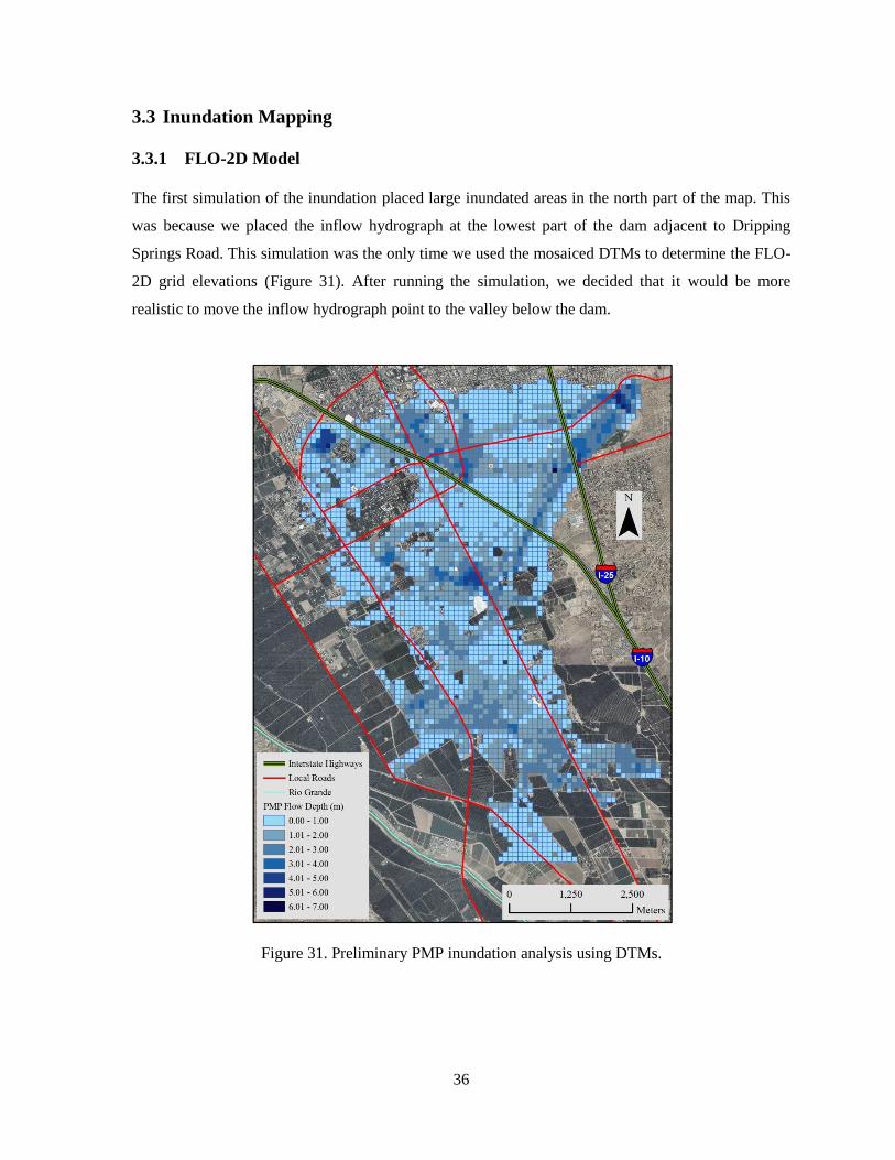
The first simulation of the inundation placed large inundated areas in the north part of the map. This
was because we placed the inflow hydrograph at the lowest part of the dam adjacent to Dripping
Springs Road. This simulation was the only time we used the mosaiced DTMs to determine the FLO-
2D grid elevations (Figure 31). After running the simulation, we decided that it would be more
realistic to move the inflow hydrograph point to the valley below the dam.
Figure 31. Preliminary PMP inundation analysis using DTMs.
37
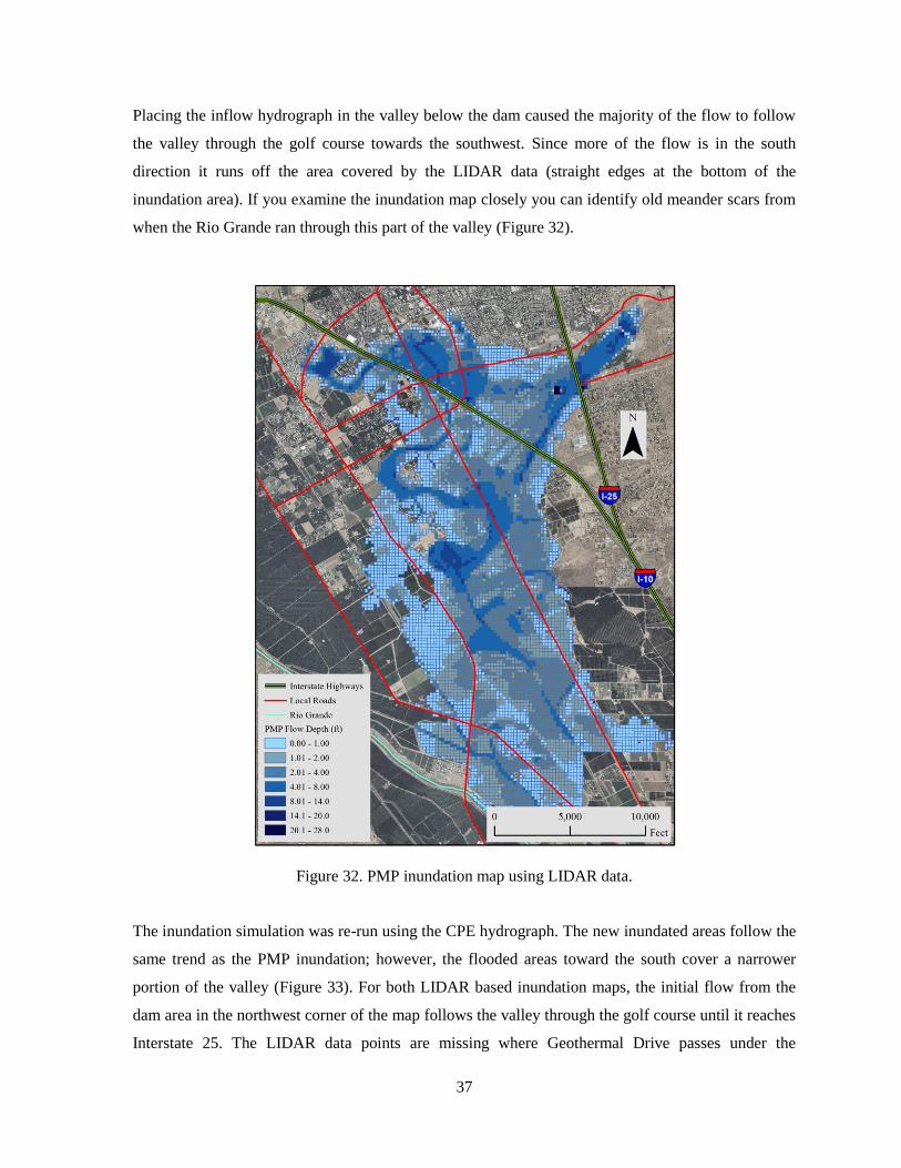
Placing the inflow hydrograph in the valley below the dam caused the majority of the flow to follow
the valley through the golf course towards the southwest. Since more of the flow is in the south
direction it runs off the area covered by the LIDAR data (straight edges at the bottom of the
inundation area). If you examine the inundation map closely you can identify old meander scars from
when the Rio Grande ran through this part of the valley (Figure 32).
Figure 32. PMP inundation map using LIDAR data.
The inundation simulation was re-run using the CPE hydrograph. The new inundated areas follow the
same trend as the PMP inundation; however, the flooded areas toward the south cover a narrower
portion of the valley (Figure 33). For both LIDAR based inundation maps, the initial flow from the
dam area in the northwest corner of the map follows the valley through the golf course until it reaches
Interstate 25. The LIDAR data points are missing where Geothermal Drive passes under the
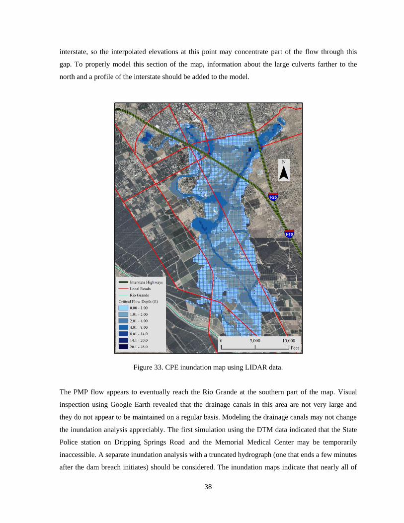
38
interstate, so the interpolated elevations at this point may concentrate part of the flow through this
gap. To properly model this section of the map, information about the large culverts farther to the
north and a profile of the interstate should be added to the model.
Figure 33. CPE inundation map using LIDAR data.
The PMP flow appears to eventually reach the Rio Grande at the southern part of the map. Visual
inspection using Google Earth revealed that the drainage canals in this area are not very large and
they do not appear to be maintained on a regular basis. Modeling the drainage canals may not change
the inundation analysis appreciably. The first simulation using the DTM data indicated that the State
Police station on Dripping Springs Road and the Memorial Medical Center may be temporarily
inaccessible. A separate inundation analysis with a truncated hydrograph (one that ends a few minutes
after the dam breach initiates) should be considered. The inundation maps indicate that nearly all of
39
New Mexico State University would need to be evacuated for both the PMP and CPE. The areas that
appear safe from inundation are the triangle formed by the intersection of Interstate 10 and Interstate
25 in the southeast part of the NMSU campus, and areas north of University Avenue between Locust
Street and Interstate 10.
The areas on both sides of Interstate 25 would need to be evacuated from NMSU west to Avenida de
Mesilla for the PMP; however, only on the north side of the interstate for the CPE. Mesilla Park and
the valley towards the south would need to be evacuated for both the PMP and CPE. Old Mesilla
lives up to its name (little table) and escapes inundation. Perhaps public schools or other public
buildings in Old Mesilla could be used as refuges for evacuees. There are also high areas paralleling
Interstate 10 along the south valley.
3.3.2 HEC-RAS Model
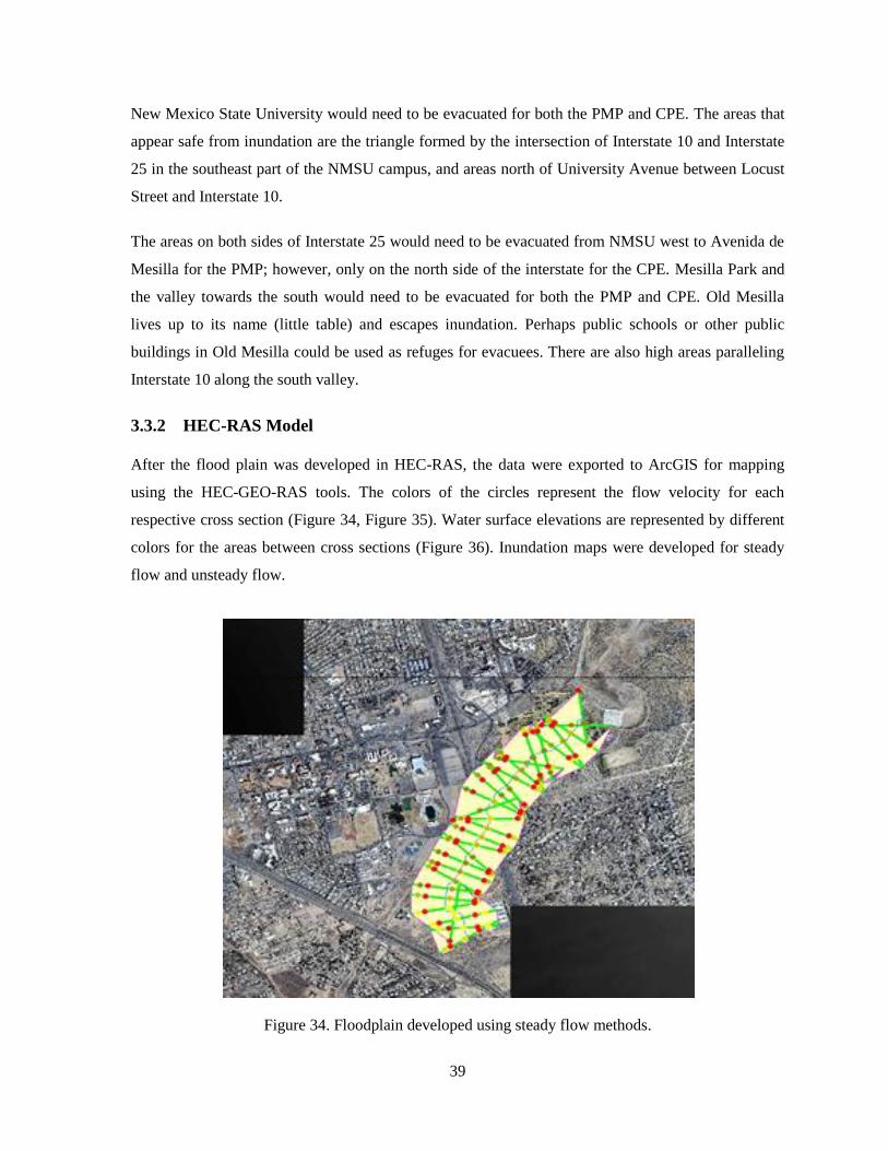
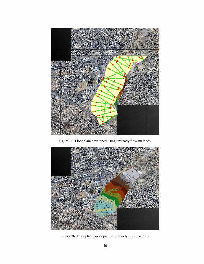
After the flood plain was developed in HEC-RAS, the data were exported to ArcGIS for mapping
using the HEC-GEO-RAS tools. The colors of the circles represent the flow velocity for each
respective cross section (Figure 34, Figure 35). Water surface elevations are represented by different
colors for the areas between cross sections (Figure 36). Inundation maps were developed for steady
flow and unsteady flow.
Figure 34. Floodplain developed using steady flow methods.
40
Figure 35. Floodplain developed using unsteady flow methods.
Figure 36. Floodplain developed using steady flow methods.
41
4 Conclusions and Recommendations
This project was intended to:
Provide Tortugas I Dam outflow hydrograph for 24 hour precipitation events with a 10, 50,
100, and 500 year return period.
Provide Tortugas I Dam outflow hydrograph for 24 hour Probable Maximum Precipitation
event and a 24 hour Critical Precipitation event dam breaches.
Provide inundation maps estimating the inundation area in the event of a dam breach from
the 24 hour Probable Maximum Precipitation event
Provide a complete engineering report describing methods and assumptions used to generate
the charts and maps as well as conclusions and recommendations related to the project
findings.
Complete a complementary CPE analysis for consideration as an alternative to the PMP
analysis.
The hydrological analysis for the 10, 50, 100, and 500 year return period precipitations events
provided useful information for local flood plain managers. The analysis reveals that at low volumes
(10 year) there is a 15 hour lag time from peak inflow to peak outflow that will allow sufficient time
for any management programs that need to be implemented. The analysis also shows that the lag time
for peak inflow and peak outflow decreases as the storm intensity increases. This means that
management plans must in place to minimize loss of property and life before these events occur. An
inundation analysis was not performed for these storms. We recommend that an inundation analysis
also be performed for the 100 and 500 year return period storms since significant road and building
development has occurred in nearby areas since the dam was constructed.
The hydrological analysis for the PMP and CPE models provided useful hydrographs which were
then used to model the dam breach and produce inundation maps. The watershed and dam breach
analysis revealed that the timing of the watershed runoff and the dam breach nearly coincide. This
indicates that an early warning system associated with dam storage elevations may not give adequate
time for an evacuation order to be issued. We recommend that an alternative method for predicting a
dam breach be implemented.
Inundation maps were produced using both HEC-RAS and FLO-2D. There were many difficulties
encountered while developing the HEC-RAS model, including the use of unrealistically narrow cross
sections at sharp channel bends and the impossibility of extending the cross section far enough for flat
regions of the flood plain. In contrast, FLO-2D appears to produce more realistic inundation maps
42
with considerably less effort (and using the same type s of data as HEC-RAS). We recommend that a
2-dimensional model of the flood plain be used in any future work.
There was no sensitivity analysis performed in this project with the exception of the comparison for
channel profiles in the watershed model. Even this was only a modest effort on one reach in the PMP
model. Several channels from the PMP and CPE should have been checked as the sensitivity of the
flow to changes in the reach cross section may vary according to flow and location in the watershed
model. Future work should include a sensitivity analysis to determine which model parameters are
most significant.
There are several assumptions we made for this study that should be revisited in future investigations.
We did not have enough information to implement a surface method in the watershed analysis so it
was neglected in this study and the discharge coefficients for the spillway flow and the dam overflow
used in the dam breach analysis were not verified.
The reaches in subbasin 1 were grossly simplified because of time constraints. This area has been
substantially modified since the DTMs were produced because of channel widening, construction of a
new high school, extension of the Sonoma Ranch Road (including bridges and culverts which can
delay flow), and the modification of the areas around the Farm and Ranch Museum. Since LIDAR
data are available for this area, we recommend running an additional FLO-2D simulation with
multiple inflow hydrographs (representing the 5 reaches contributing to the flow across the subbasin).
We initially modeled the inundation areas with FLO-2D expecting the breach to occur just east of
Dripping Springs Road. In this scenario, the Memorial Medical Center and surrounding facilities
would be flooded. We later realized that the breach would quickly erode a channel closer to the center
of the valley and shift the flow towards the golf course. Even though the duration of the flow towards
the medical center would be relatively brief, the large quantities of water spilling through the breach
could still threaten the medical facilities. We recommend that a separate inundation analysis be
performed for this area using a truncated outflow hydrograph.
One frightening aspect revealed by the analysis is that any dam breach will cause major water flows
to come in contact with a closed landfill on the New Mexico State University property. We
recommend that an investigation be initiated to determine whether hazardous materials are stored in
the landfill, and to determine what the consequences would be if the landfill were disturbed by a
flood.

43
The inundation maps produced using the FLO-2D model for the PMP and the CPE had similar
inundation areas. This initial observation indicates that using the CPE may be a useful alternative to
using the PMP for inundation mapping, and evacuation planning. We recommend that future work
include an investigation into the consequences of using the CPE instead of the PMP for evacuation
planning.
44
References
Aquaveo. SMS Learning Center. http://www.aquaveo.com/sms-learning (Accessed September, 2012).
Chin, David. (2006). Water-resources engineering. (2nd ed.). Upper Saddle River, NJ: Prentice Hall.
Ciolli, M. Grass tutorial. Universita Degli Studi Di Trento.
http://www.ing.unitn.it/~grass/docs/tutorial_62_en/htdocs/esercitazione/dtm/dtm4.html
(Accessed September 2012).
Croley II, Thomas E., (2001). Climate-Biased Storm-Frequency Estimation. Journal of Hydrologic
Engineering. Retrieved from http://www.glerl.noaa.gov/pubs/fulltext/2001/20010002.pdf
EPA. Environmental Protection Agency 2006 National Land Cover Data maps.
http://www.epa.gov/mrlc/nlcd-2006.html (Accessed September, 2012).
ESRI® ArcMap™ 10.0. ESRI Inc. Redmond, CA, USA.
Forest Service. Fusion version 3.20. [Software]. USDA Forest Service.
http://forsys.cfr.washington.edu/fusion/fusion320.html (Accessed September, 2012).
Fry, J., Xian, G., Jin, S., Dewitz, J., Homer, C., Yang, L., Barnes, C., Herold, N., and Wickham, J.,
(2011). Completion of the 2006 National Land Cover Database for the Conterminous United
States, PE&RS, Vol. 77(9):858-864.
Google Inc. (2009). Google Earth (Version 5.1.3533.1731) [Software]. Available from
http://www.linguistics.ucla.edu/people/hayes/otsoft/
GRASS Development Team, 2011. GRASS 6.4 Users Manual. Open Source Geospatial Foundation,
USA. Electronic document: http://grass.osgeo.org/grass64/manuals/html64_user/ (Accessed
September 2012).
GRASS Development Team, 2012. Geographic Resources Analysis Support System (GRASS)
Software, Version 6.4. [Software].
FLO-2D. (2012). FLO-2D Version 2009.06. FLO-2D Software, Inc. [Software].
HEC-HMS. (2010). Hydrologic modeling system HEC-HMS. Davis, CA: U.S. Army Corps of
Engineers Hydrologic Engineering Center, HEC.
HEC-RAS. (2010). HEC-RAS river analysis system. Davis, CA: U.S. Army Corps of Engineers,
Institute for Water Resources, Hydrologic Engineering Center, HEC.
Meyer, S., and F. Olivera. (2007). Floodplain Mapping & Hydraulic Analysis with HEC-GeoRAS
4.1.1 and ArcGIS 9.1.

45
NRCS. Natural Resource Conservation Service soil survey. (n.d.). Retrieved from
http://websoilsurvey.nrcs.usda.gov/app/WebSoilSurvey.aspx (Accessed September, 2012).
NRCS. U.S. Department of Agriculture, Natural Resource Conservation Service (n.d.). SCS
Engineering Field Handbook. (Chapter 2) Retrieved from
http://policy.nrcs.usda.gov/OpenNonWebContent.aspx?content=17541.wba (Accessed October,
2012).
NOAA. U.S. Department of Commerce, National Oceanic and Atmospheric Administration, National
Weather Service. Hydrometeorological Design Studies Center.
http://www.nws.noaa.gov/oh/hdsc/index.html (Accessed September, 2012).
[Rainfall Distribution Curve] Retrieved October 2012, from
http://forest.mtu.edu/pcforestry/resources/studentprojects/scs/
Rendon, S.H., Ashworth, C.E., and Smith, S.J. (2012). Dam-breach analysis and flood-inundation
mapping for Lakes Ellsworth and Lawtonka near Lawton, Oklahoma: U.S. Geological Survey
Scientific Investigations Report 2012–5026, 56 p.
RGIS. New Mexico Resource Geographic Information System Program. http://rgis.unm.edu/
(Accessed September, 2012).
USDA. WinTR-55 Watershed Hydrology [Software].
http://www.nrcs.usda.gov/wps/portal/nrcs/detailfull/national/water/quality/?&cid=stelprdb104290
1 (Accessed September, 2012).
[U.S. Type Storms map] Retrieved October 2012, from http://www.ems-
i.com/wmshelp/Hydrologic_Models/Models/HMS/Meteorological_Parameters/SCS_Hypothetical
_Storm.htm
46
Appendix
Table 6. Subbasin data.
Subbasin
Outlet
Easting (m) Northing (m) Area (km2)
Tortugas_I_Subbasin_1 337215.72 3574145.13 4.13
Tortugas_I_Subbasin_1_2 338235.58 3575744.49 1.19
Tortugas_I_Subbasin_1_3 338505.62 3575465.94 2.49
Tortugas_I_Subbasin_1_4 339505.68 3575134.67 1.64
Tortugas_I_Subbasin_1_5 339085.64 3574603.84 0.56
Tortugas_I_Subbasin_1_3_6 339195.65 3577266.47 1.57
Tortugas_I_Subbasin_1_3_7 339805.48 3576856.31 1.65
Tortugas_I_Subbasin_1_3_8 339787.09 3576344.77 2.16
Tortugas_I_Subbasin_1_3_7_9 341636.18 3578274.79 1.83
Tortugas_I_Subbasin_1_4_10 339564.93 3575124.69 2.40
Tortugas_I_Subbasin_1_4_11 339623.35 3575065.79 3.01
Tortugas_I_Subbasin_1_4_10_12 341924.72 3576865.14 2.70
Tortugas_I_Subbasin_1_4_10_13 342156.29 3576584.77 1.00
Tortugas_I_Subbasin_1_4_10_13_14 342305.32 3576465.00 1.02
Tortugas_I_Subbasin_1_4_10_13_14_15 343025.37 3576383.53 2.46
Tortugas_I_Subbasin_1_4_10_12_16 344885.22 3578805.16 2.05
Tortugas_I_Subbasin_1_4_10_13_14_17 345055.20 3577924.77 0.38
Tortugas_I_Subbasin_1_4_10_13_14_15_18 345884.01 3578025.07 1.72
Tortugas_I_Subbasin_1_4_10_12_16_19 347753.98 3579185.19 0.49
Tortugas_I_Subbasin_1_4_10_12_16_19_20 349315.86 3578834.73 0.60
Tortugas_I_Subbasin_1_4_11_21 342774.80 3575164.97 3.07
Tortugas_I_Subbasin_1_4_11_21_22 346095.56 3576875.46 3.75
Tortugas_I_Subbasin_1_4_11_21_23 346004.62 3576535.18 1.05
Tortugas_I_Subbasin_1_4_10_12_16_19_20_24 350885.79 3579285.25 0.93
Tortugas_I_Subbasin_1_4_10_12_16_19_20_25 350500.91 3578835.56 4.91
Tortugas_I_Subbasin_1_4_10_12_16_19_20_26 349444.11 3578765.04 1.05
Tortugas_I_Subbasin_1_4_10_12_16_19_20_26_27 350474.93 3578074.84 1.65
Tortugas_I_Subbasin_1_4_10_12_16_19_20_26_28 351445.66 3577304.07 2.08
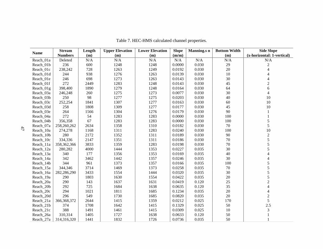
47
Table 7. HEC-HMS calculated channel properties.
Name Stream
Numbers
Length
(m)
Upper Elevation
(m)
Lower Elevation
(m)
Slope
(m/m)
Manning.s n Bottom Width
(m)
Side Slope
(x-horizontal: 1-vertical)
Reach_01a Deleted N/A N/A N/A N/A N/A N/A N/A
Reach_01b 236 600 1248 1248 0.0000 0.030 29 2
Reach_01c 238,242 728 1263 1249 0.0192 0.030 20 4
Reach_01d 244 938 1276 1263 0.0139 0.030 10 4
Reach_01e 246 698 1273 1263 0.0143 0.030 30 4
Reach_01f 272 2449 1283 1248 0.0143 0.030 45 2
Reach_01g 398,400 1890 1279 1248 0.0164 0.030 64 6
Reach_03a 246,248 260 1275 1273 0.0077 0.030 30 4
Reach_03b 250 98 1277 1275 0.0203 0.030 40 10
Reach_03c 252,254 1841 1307 1277 0.0163 0.030 60 10
Reach_03d 258 1808 1309 1277 0.0177 0.030 45 10
Reach_03e 264 1566 1304 1276 0.0179 0.030 90 1
Reach_04a 272 54 1283 1283 0.0000 0.030 100 1
Reach_04b 356,358 67 1283 1283 0.0000 0.030 100 5
Reach_07a 258,260,262 2634 1358 1310 0.0182 0.030 70 5
Reach_10a 274,278 1168 1311 1283 0.0240 0.030 100 10
Reach_10b 280 2172 1352 1311 0.0189 0.030 90 2
Reach_10c 334,336 2147 1351 1311 0.0186 0.030 70 5
Reach_11a 358,362,366 3833 1359 1283 0.0198 0.030 70 5
Reach_12a 280,282 4000 1444 1353 0.0227 0.035 30 5
Reach_13a 340 177 1356 1353 0.0169 0.035 40 4
Reach_14a 342 3462 1442 1357 0.0246 0.035 30 4
Reach_14b 344 961 1373 1357 0.0166 0.035 100 5
Reach_15a 344,346 3714 1469 1373 0.0258 0.035 70 5
Reach_16a 282,286,290 3433 1554 1444 0.0320 0.035 30 5
Reach_19a 290 1803 1630 1554 0.0422 0.035 20 5
Reach_20a 290 143 1637 1631 0.0419 0.120 25 2
Reach_20b 292 725 1684 1638 0.0635 0.120 35 4
Reach_20c 294 1021 1811 1685 0.1234 0.035 20 4
Reach_20d 296 549 1730 1685 0.0820 0.035 20 2
Reach_21a 366,368,372 2644 1415 1359 0.0212 0.025 170 5
Reach_21b 374 1708 1642 1415 0.1329 0.025 50 2.5
Reach_21c 388 1491 1461 1415 0.0309 0.025 10 3
Reach_26a 310,314 1405 1727 1638 0.0633 0.120 50 1
Reach_27a 314,316,320 1441 1832 1726 0.0736 0.035 50 1
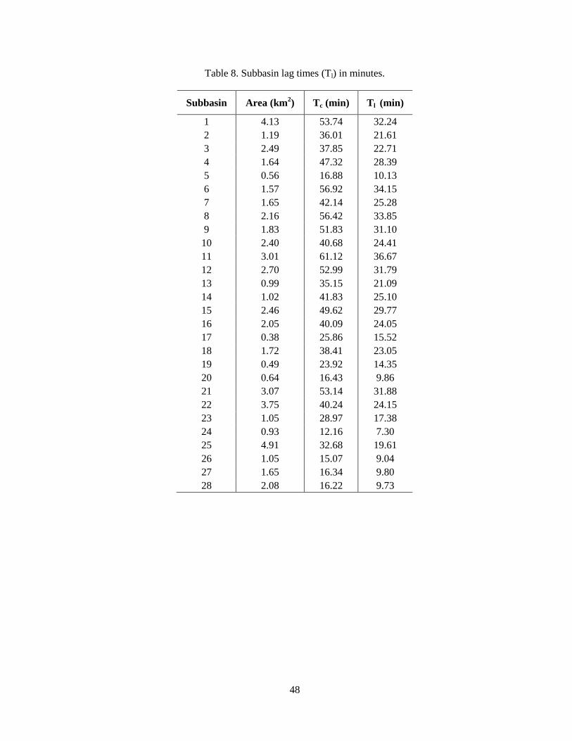
48
Table 8. Subbasin lag times (Tl) in minutes.
Subbasin Area (km2) Tc (min) Tl (min)
1 4.13 53.74 32.24
2 1.19 36.01 21.61
3 2.49 37.85 22.71
4 1.64 47.32 28.39
5 0.56 16.88 10.13
6 1.57 56.92 34.15
7 1.65 42.14 25.28
8 2.16 56.42 33.85
9 1.83 51.83 31.10
10 2.40 40.68 24.41
11 3.01 61.12 36.67
12 2.70 52.99 31.79
13 0.99 35.15 21.09
14 1.02 41.83 25.10
15 2.46 49.62 29.77
16 2.05 40.09 24.05
17 0.38 25.86 15.52
18 1.72 38.41 23.05
19 0.49 23.92 14.35
20 0.64 16.43 9.86
21 3.07 53.14 31.88
22 3.75 40.24 24.15
23 1.05 28.97 17.38
24 0.93 12.16 7.30
25 4.91 32.68 19.61
26 1.05 15.07 9.04
27 1.65 16.34 9.80
28 2.08 16.22 9.73
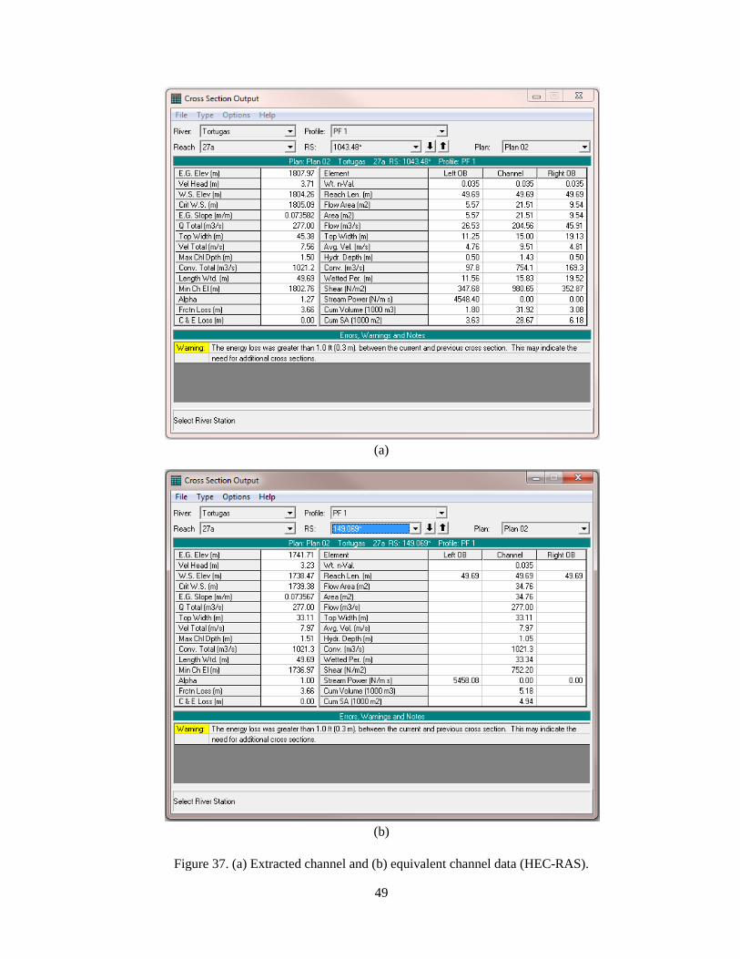
49
(a)
(b)
Figure 37. (a) Extracted channel and (b) equivalent channel data (HEC-RAS).
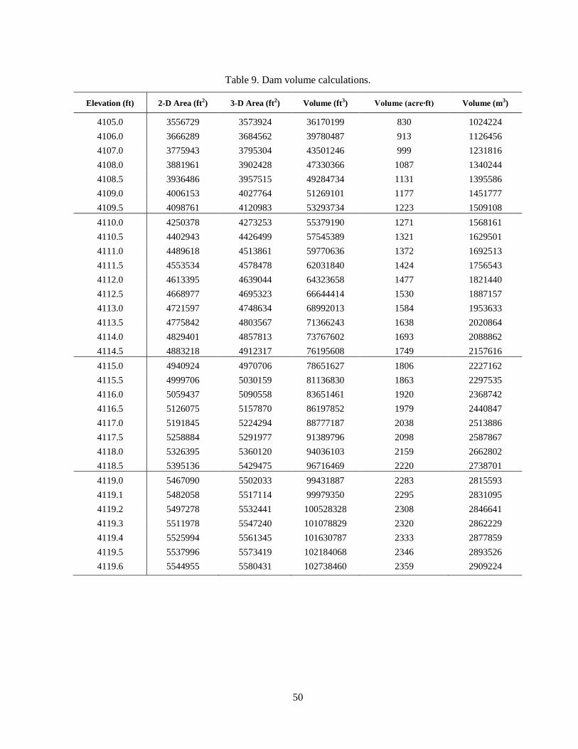
50
Table 9. Dam volume calculations.
Elevation (ft) 2-D Area (ft2) 3-D Area (ft2) Volume (ft3) Volume (acre∙ft) Volume (m3)
4105.0 3556729 3573924 36170199 830 1024224
4106.0 3666289 3684562 39780487 913 1126456
4107.0 3775943 3795304 43501246 999 1231816
4108.0 3881961 3902428 47330366 1087 1340244
4108.5 3936486 3957515 49284734 1131 1395586
4109.0 4006153 4027764 51269101 1177 1451777
4109.5 4098761 4120983 53293734 1223 1509108
4110.0 4250378 4273253 55379190 1271 1568161
4110.5 4402943 4426499 57545389 1321 1629501
4111.0 4489618 4513861 59770636 1372 1692513
4111.5 4553534 4578478 62031840 1424 1756543
4112.0 4613395 4639044 64323658 1477 1821440
4112.5 4668977 4695323 66644414 1530 1887157
4113.0 4721597 4748634 68992013 1584 1953633
4113.5 4775842 4803567 71366243 1638 2020864
4114.0 4829401 4857813 73767602 1693 2088862
4114.5 4883218 4912317 76195608 1749 2157616
4115.0 4940924 4970706 78651627 1806 2227162
4115.5 4999706 5030159 81136830 1863 2297535
4116.0 5059437 5090558 83651461 1920 2368742
4116.5 5126075 5157870 86197852 1979 2440847
4117.0 5191845 5224294 88777187 2038 2513886
4117.5 5258884 5291977 91389796 2098 2587867
4118.0 5326395 5360120 94036103 2159 2662802
4118.5 5395136 5429475 96716469 2220 2738701
4119.0 5467090 5502033 99431887 2283 2815593
4119.1 5482058 5517114 99979350 2295 2831095
4119.2 5497278 5532441 100528328 2308 2846641
4119.3 5511978 5547240 101078829 2320 2862229
4119.4 5525994 5561345 101630787 2333 2877859
4119.5 5537996 5573419 102184068 2346 2893526
4119.6 5544955 5580431 102738460 2359 2909224
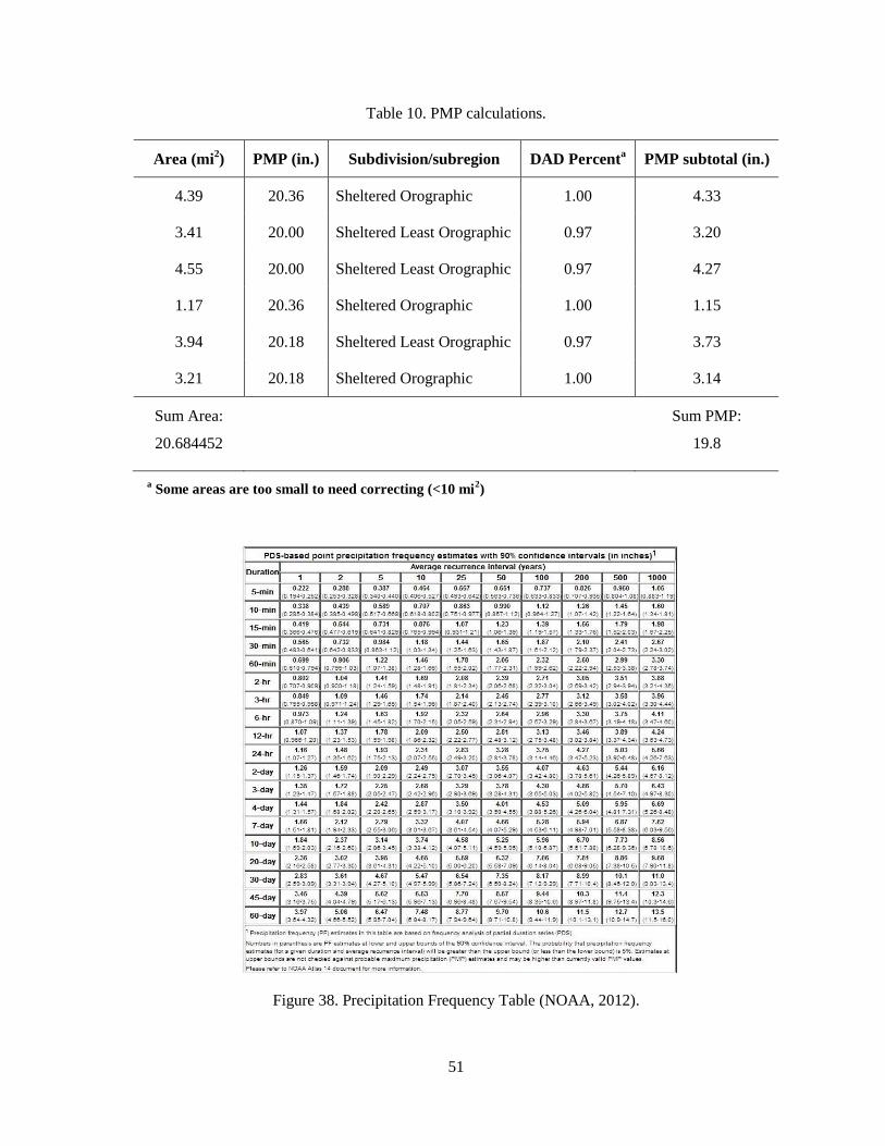
51
Table 10. PMP calculations.
Area (mi2) PMP (in.) Subdivision/subregion DAD Percent
a PMP subtotal (in.)
4.39 20.36 Sheltered Orographic 1.00 4.33
3.41 20.00 Sheltered Least Orographic 0.97 3.20
4.55 20.00 Sheltered Least Orographic 0.97 4.27
1.17 20.36 Sheltered Orographic 1.00 1.15
3.94 20.18 Sheltered Least Orographic 0.97 3.73
3.21 20.18 Sheltered Orographic 1.00 3.14
Sum Area:
20.684452
Sum PMP:
19.8
a Some areas are too small to need correcting (<10 mi
2)
Figure 38. Precipitation Frequency Table (NOAA, 2012).