A (very) shortintroduction to R

Paul Torfs & Claudia BrauerHydrology and Quantitative Water Management Group

Wageningen University, The Netherlands

16 April 2012

1 Introduction

R is a powerful language and environment for sta-tistical computing and graphics. It is a public do-main (a so called “GNU”) project which is similarto the commercial S language and environmentwhich was developed at Bell Laboratories (for-merly AT&T, now Lucent Technologies) by JohnChambers and colleagues. R can be considered asa different implementation of S, and is much usedin as an educational language and research tool.

The main advantages of R are the fact that Ris freeware and that there is a lot of help avail-able. It is quite similar to other programmingpackages such as MatLab (not freeware), but moreuser-friendly than programming languages such asC++ or Fortran. You can use R as it is, but foreducational purposes we prefer to use R in combi-nation with the RStudio interface (also freeware),which has an organized layout and several extraoptions.

2 Getting started

2.1 Install R

To install R on your computer (legally for free!),go to the home website of R:

http://www.r-project.org/

and do the following (assuming you work on awindows computer):• click download CRA in the left bar• choose a download site• choose Windows as target operation system• click base

• choose Download R 2.14.1 for Windows ∗

and choose default answers for all questions

It is also possible to run R and RStudio froma USB stick instead of installing them. Thiscould be useful when you don’t have administra-tor rights on your computer. See our separate note“How to use portable versions of R and RStudio”for help on this topic.

2.2 Install RStudio

After finishing this setup, you should see an ”R”icon on you desktop. Clicking on this would startup the standard interface. We recommend, how-ever, to use the RStudio interface. † To installRStudio, go to:

http://www.rstudio.org/

and do the following (assuming you work on a win-dows computer):• click Download RStudio

• click Download RStudio Desktop

• click Recommended For Your System

• download the .exe file and run it (choose defaultanswers for all questions)

2.3 RStudio layout

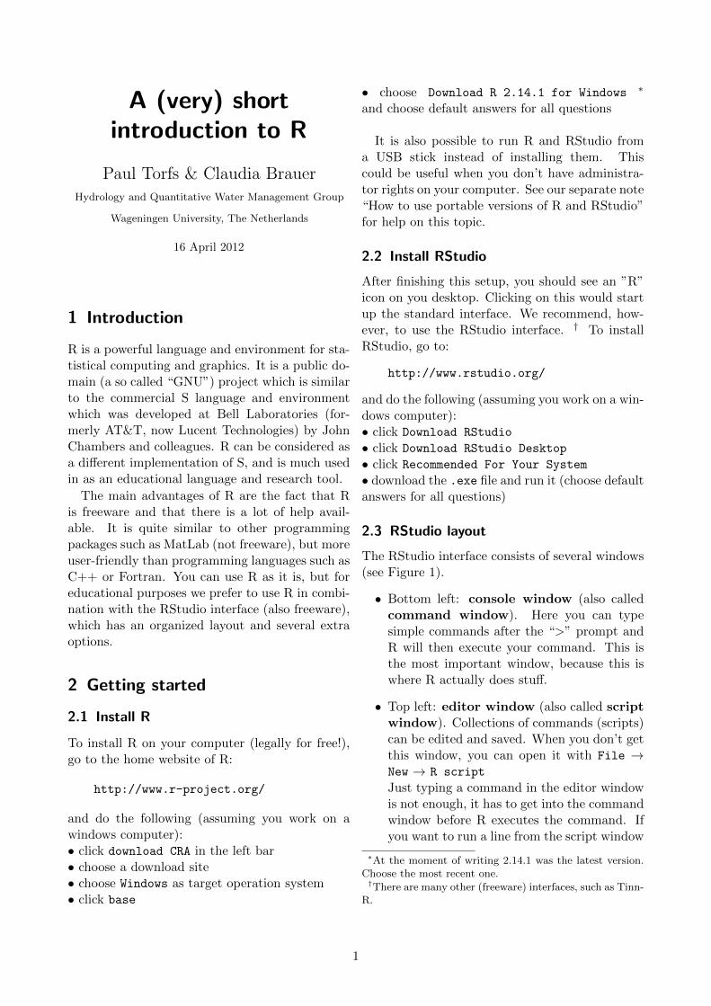
The RStudio interface consists of several windows(see Figure 1).

• Bottom left: console window (also calledcommand window). Here you can typesimple commands after the “>” prompt andR will then execute your command. This isthe most important window, because this iswhere R actually does stuff.

• Top left: editor window (also called scriptwindow). Collections of commands (scripts)can be edited and saved. When you don’t getthis window, you can open it with File →New → R script

Just typing a command in the editor windowis not enough, it has to get into the commandwindow before R executes the command. Ifyou want to run a line from the script window

∗At the moment of writing 2.14.1 was the latest version.Choose the most recent one.†There are many other (freeware) interfaces, such as Tinn-

R.

1

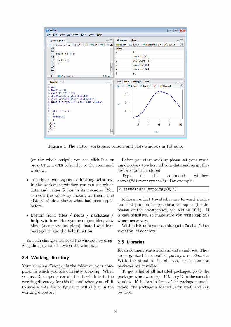
Figure 1 The editor, workspace, console and plots windows in RStudio.

(or the whole script), you can click Run orpress CTRL+ENTER to send it to the commandwindow.

• Top right: workspace / history window.In the workspace window you can see whichdata and values R has in its memory. Youcan edit the values by clicking on them. Thehistory window shows what has been typedbefore.

• Bottom right: files / plots / packages /help window. Here you can open files, viewplots (also previous plots), install and loadpackages or use the help function.

You can change the size of the windows by drag-ging the grey bars between the windows.

2.4 Working directory

Your working directory is the folder on your com-puter in which you are currently working. Whenyou ask R to open a certain file, it will look in theworking directory for this file and when you tell Rto save a data file or figure, it will save it in theworking directory.

Before you start working please set your work-ing directory to where all your data and script filesare or should be stored.

Type in the command window:setwd("directoryname"). For example:

> setwd("M:/Hydrology/R/")

Make sure that the slashes are forward slashesand that you don’t forget the apostrophes (for thereason of the apostrophes, see section 10.1). Ris case sensitive, so make sure you write capitalswhere necessary.

Within RStudio you can also go to Tools / Set

working directory.

2.5 Libraries

R can do many statistical and data analyses. Theyare organized in so-called packages or libraries.With the standard installation, most commonpackages are installed.

To get a list of all installed packages, go to thepackages window or type library() in the consolewindow. If the box in front of the package name isticked, the package is loaded (activated) and canbe used.

2

There are many more packages available on theR-website. If you want to install and use a pack-age (for example, the package called “geometry”)you should:• Install the package: click install packages

in the packages window and type geometry

or type install.packages("geometry") in thecommand window.• Load the package: check box in front ofgeometry or type library("geometry") in thecommand window.

3 Some first examples of Rcommands

3.1 Calculator

R can be used as an calculator. You can just typeyour equation in the command window after the“>”:

> 10^2 + 36

and R will give the answer

[1] 136

ToDo

Compute the difference between 2012 and theyear you started at this university and dividethis by the difference between 2012 and the yearyou were born. Multiply this with 100 to getthe percentage of your life you have spent atthis university. Use brackets if you need them.

If you use brackets and forget to add the closingbracket, the “>” on the command line changesinto a “+”. The “+” can also mean that R is stillbusy with some heavy computation. If you wantR to quit what it was doing and give back the “>”,press ESC.

3.2 Workspace

You can also give numbers a name. By doing so,they become so-called variables which can be usedlater. For example, you can type in the commandwindow:

> a = 4

You can see that a appears in the workspacewindow, which means that R now rememberswhat a is. You can also ask R what a is (justtype a ENTER in the command window):

> a

[1] 4

or do calculations with a:

> a * 5

[1] 20

If you specify a again, it will forget what valueit had before. You can also assign a new value toa using the old one.

> a = a + 1

> a

[1] 21

To remove all variables from R’s memory, type

> rm(list=ls())

or click “clear all” in the workspace window. Youcan see that RStudio then empties the workspacewindow. If you only want to remove the variablea, you can type rm(a).

ToDo

Repeat the previous ToDo, but with severalsteps in between. You can give the variablesany name you want, but the name has to startwith a letter.

3.3 Scalars, vectors and matrices

Like in many other programs, R organizes num-bers in scalars (a single number — 0-dimensional),vectors (a row of numbers, also called arrays —1-dimensional) and matrices (like a table — 2-dimensional).

The a you defined before was a scalar. To definea vector with the numbers 3, 4 and 5, you need thefunction‡ c, which is short for concatenate (pastetogether).

b=c(3,4,5)

Matrices and other 2-dimensional structureswill be introduced in Section 6.‡See next Section for the explanation of functions.

3

3.4 Functions

If you would like to compute the mean of all theelements in the vector b from the example above,you could type

> (3+4+5)/3

But when the vector is very long, this is very bor-ing and time-consuming work. This is why thingsyou do often are automated in so-called functions.Some functions are standard in R or in one of thepackages. You can also program your own func-tions (Section 11.3). When you use a function tocompute a mean, you’ll type:

> mean(x=b)

Within the brackets you specify the arguments.Arguments give extra information to the function.In this case, the argument x says of which setof numbers (vector) the mean should computed(namely of b). Sometimes, the name of the argu-ment is not necessary: mean(b) works as well.

ToDo

Compute the sum of 4, 5, 8 and 11 by first com-bining them into a vector and then using thefunction sum.

The function rnorm, as another example, is astandard R function which creates random sam-ples from a normal distribution. Hit the ENTER

key and you will see 10 random numbers as:

1 > rnorm(10)

2 [1] -0.949 1.342 -0.474 0.403

3 [5] -0.091 -0.379 1.015 0.740

4 [9] -0.639 0.950

• Line 1 contains the command: rnorm is the func-tion and the 10 is an argument specifying the num-ber of random numbers you want — in this case10 numbers (typing n=10 instead of just 10 wouldalso work).• Lines 2-4 contain the results: 10 random num-bers organised in a vector with length 10.

Entering the same command again produces 10new random numbers. Instead of typing the sametext again, you can also press the upward arrowkey (↑). If you want 10 random numbers out ofnormal distribution with mean 1.2 and standarddeviation 3.4 you can type

> rnorm(10, mean=1.2, sd=3.4)

showing that the same function (rnorm) may havedifferent interfaces and that R has so called namedarguments’ (in this case mean and sd). By the way,the spaces around the “,” and “=” do not matter.

Comparing this example to the previous onealso shows that for the function rnorm only thefirst argument (the number 10) is compulsory, andthat R gives default values to the other so-calledoptional arguments.§

RStudio has a nice feature: when you typernorm( in the command window and press TAB,RStudio will show the possible arguments (Fig-ure 2).

3.5 Plots

R can make graphs. The following is a very sim-ple ¶ example:

1 > x = rnorm(100)

2 > x

3 > plot(x)

• In the first line, 100 random numbers areassigned to the variable x, which becomes avector by this operation.• The second line will show these numbers on thescreen.• In the third line, all these values are plotted inthe plots window.

ToDo

Plot 100 normal random numbers.

4 Help and documentation

There is a large amount of (free) documentationand help available. Some help is automaticallyinstalled. Typing in the console window the com-mand

> help(rnorm)

§Use the help function (Section 4) to see which values areused as default.¶See Section 7 for slightly less trivial examples.

4

Figure 2 RStudio shows possible arguments when you press TAB after the function name and bracket.

gives help on the rnorm function. It gives a de-scription of the function, possible arguments andthe values that are used as default for optionalarguments. Typing

> example(rnorm)

gives some examples of how the function can beused.

An HTML-based global help can be called with:

> help.start()

or by going to the help window.The following links can also be very useful:• http://cran.r-project.org/doc/manuals/

R-intro.pdf A full manual.• http://cran.r-project.org/doc/contrib/

Short-refcard.pdf A short reference card.• http://zoonek2.free.fr/UNIX/48 R/all.html

A very rich source of examples.• http://rwiki.sciviews.org/doku.phpA typical user wiki.• http://www.statmethods.net/Also called Quick-R. Gives very productivedirect help. Also for users coming from otherprogramming languages.• http://mathesaurus.sourceforge.net/Dictionary for programming languages (e.g. R forMatlab users).• Just using Google (type e.g. “R rnorm” in thesearch field) can also be very productive.

ToDo

Find help for the sqrt function.

5 Scripts

R is an interpreter that uses a command linebased environment. This means that you have totype commands, rather than using the mouse andmenus. This has the advantage that you do notalways have to retype all commands and are lesslikely to get RSI.

You can store your commands in files, the so-called scripts. These scripts have typically filenames with the extension .R, e.g. foo.R. You canopen an editor window to edit these files by click-ing File and New or Open file... ‖.

You can run (send to the console window)part of the code by selecting lines and pressingCTRL+ENTER or click Run in the editor window.You can always run the whole script with the con-sole command source, so e.g. for the script in thefile foo.R you type:

> source("foo.R")

You can also click Run all in the editor windowto run the whole script at once.

ToDo

Make a file called firstscript.R containing R-code that generates 300 random normal num-bers and plots them, and run this script severaltimes.

‖Where also the options Save and Save as are available.

5

6 Data structures

If you are unfamiliar with R, it makes sense tojust retype the commands listed in this section.Maybe you will not need all these structures inthe beginning, but it is always good to have atleast a first glimpse of the terminology and use ofthese.

6.1 Vectors

Vectors were already introduced, but they can domore:

1 > vec1 = c(1,4,6,8,10)

2 > vec1

3 [1] 1 4 6 8 10

4 > vec1[5]

5 [1] 10

6 > vec1[3] = 12

7 > vec1

8 [1] 1 4 12 8 10

9 > vec2 = seq(from=0, to=1, length=5)

10 > vec2

11 [1] 0.00 0.25 0.50 0.75 1.00

12 > sum(vec2)

13 [1] 29

14 > vec1 + vec2

15 [1] 1.00 4.25 12.50 8.75 11.00

• In line 1, a vector vec1 is explicitly constructedby the concatenation function c(), which was in-troduced before. Elements in vectors can be ad-dressed by standard [i] indexing, as shown inlines 4-5.• In line 6, one of the elements is replaced with anew number. The result is shown in line 8.• Line 9 demonstrates another useful way of con-structing a vector: the seq() (sequence) function.• Lines 10-15 show some typical vector orientedcalculations. Note that the function sum sums upthe elements within a vector, where if you add uptwo vectors of the same length, the first elementsof both vectors are summed, and the second ele-ments, etc., leading to a new vector of length 5(just like in regular vector calculus).

6.2 Matrices

Matrices are nothing more than 2-dimensionalvectors. To define a matrix, use the functionmatrix:

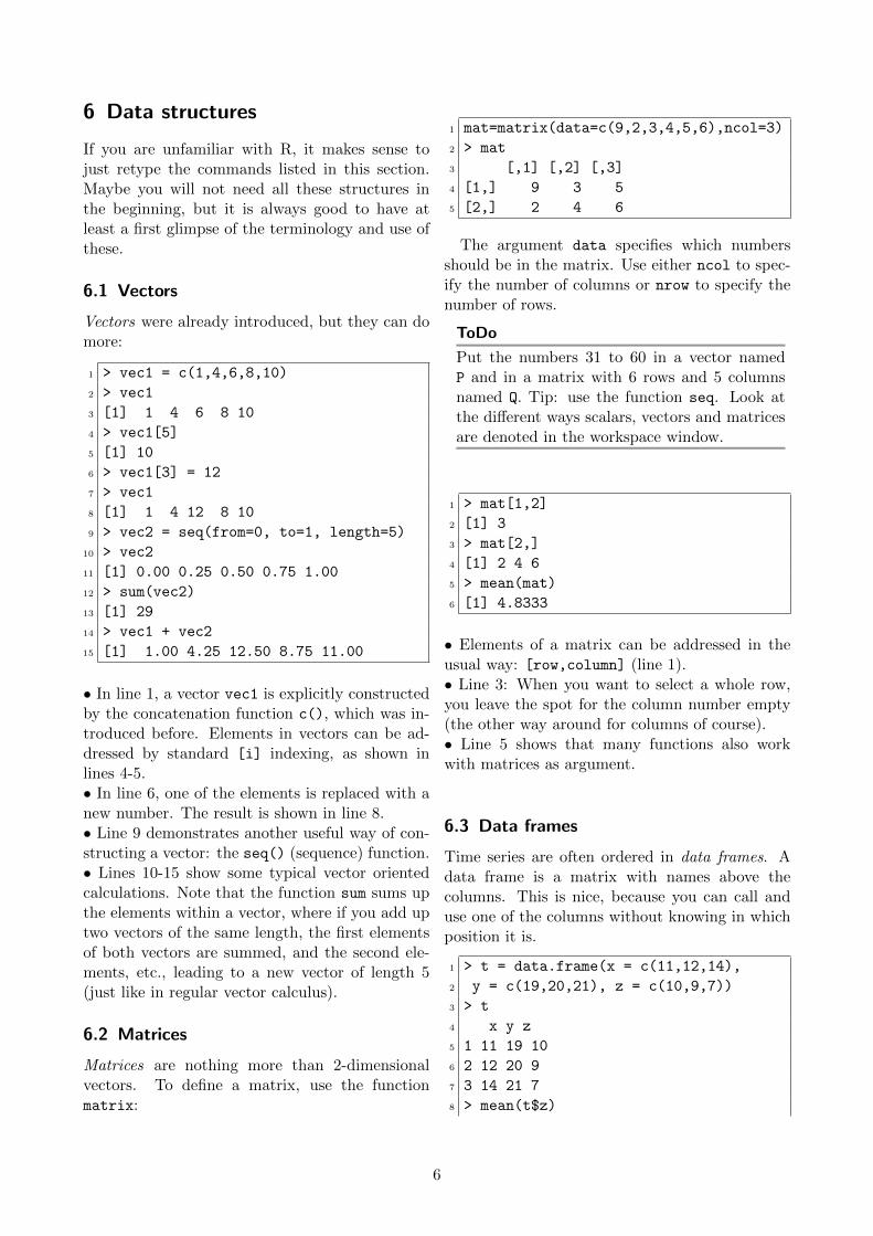
1 mat=matrix(data=c(9,2,3,4,5,6),ncol=3)

2 > mat

3 [,1] [,2] [,3]

4 [1,] 9 3 5

5 [2,] 2 4 6

The argument data specifies which numbersshould be in the matrix. Use either ncol to spec-ify the number of columns or nrow to specify thenumber of rows.

ToDo

Put the numbers 31 to 60 in a vector namedP and in a matrix with 6 rows and 5 columnsnamed Q. Tip: use the function seq. Look atthe different ways scalars, vectors and matricesare denoted in the workspace window.

1 > mat[1,2]

2 [1] 3

3 > mat[2,]

4 [1] 2 4 6

5 > mean(mat)

6 [1] 4.8333

• Elements of a matrix can be addressed in theusual way: [row,column] (line 1).• Line 3: When you want to select a whole row,you leave the spot for the column number empty(the other way around for columns of course).• Line 5 shows that many functions also workwith matrices as argument.

6.3 Data frames

Time series are often ordered in data frames. Adata frame is a matrix with names above thecolumns. This is nice, because you can call anduse one of the columns without knowing in whichposition it is.

1 > t = data.frame(x = c(11,12,14),

2 y = c(19,20,21), z = c(10,9,7))

3 > t

4 x y z

5 1 11 19 10

6 2 12 20 9

7 3 14 21 7

8 > mean(t$z)

6

9 [1] 8.666667

10 > mean(t[["z"]])

11 [1] 8.666667

• In lines 1-2 a typical data frame is constructed.The columns have the names x, y and z.• Line 8-11 show two ways of how you can selectone of the columns.

ToDo

Make a script file which constructs three ran-dom normal vectors of length 100. Call thesevectors x1, x2 and x3. Make a data frame calledt with three columns (called a, b and c) con-taining respectively x1, x1+x2 and x1+x2+x3.Call the following functions for this data frame:plot(t) and sd(t). Can you understand theresults? Rerun this script a few times.

6.4 Lists

Another basic structure in R is a list. The mainadvantage of lists is that the “columns” (they’renot really ordered in columns any more, but aremore a collection of vectors) don’t have to be ofthe same length, unlike matrices and data frames.

1 > L = list(one=1, two=c(1,2),

2 five=seq(1, 4, length=5))

3 > L

4 $one

5 [1] 1

6 $two

7 [1] 1 2

8 $five

9 [1] 1.00 1.75 2.50 3.25 4.00

10 > names(L)

11 [1] "one" "two" "five"

12 > L$five + 10

13 [1] 11.00 11.75 12.50 13.25 14.00

• Lines 1-2 construct a list by giving names andvalues. The list also appears in the workspacewindow.• Lines 3-9 show a typical printing.• Line 10 illustrates how to get all the names.• Line 12 shows how to use the numbers.

7 Graphics

The following lines show a simple plot:

> plot(rnorm(100), type="l", col="gold")

Hundred random numbers are plotted by connect-ing the points by lines (the symbol between quotesafter the type=, is the letter l, not the number 1)in a gold color.

Plotting is an important statistical activity. Soit should not come as a surprise that R has manyplotting facilities.

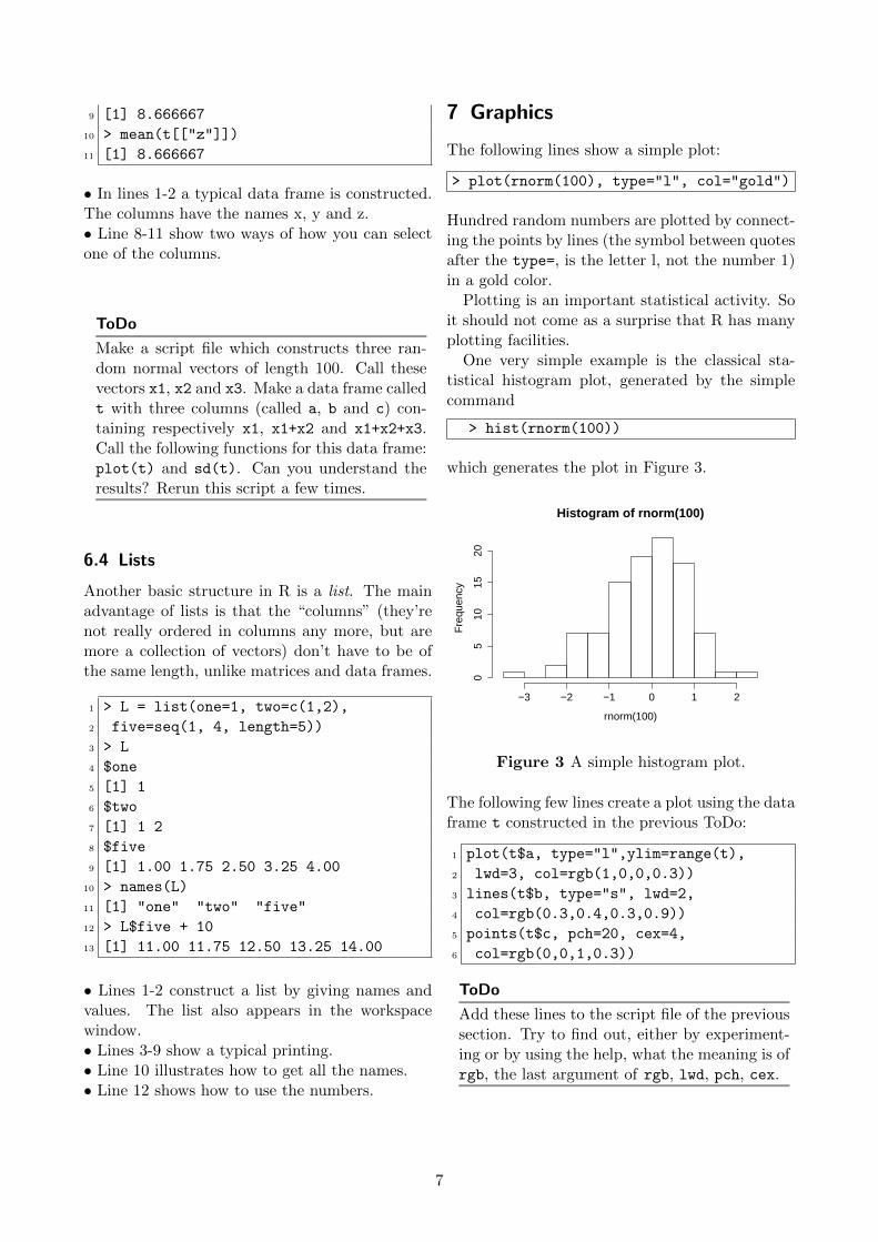
One very simple example is the classical sta-tistical histogram plot, generated by the simplecommand

> hist(rnorm(100))

which generates the plot in Figure 3.

Histogram of rnorm(100)

rnorm(100)

Fre

quen

cy

−3 −2 −1 0 1 2

05

1015

20

Figure 3 A simple histogram plot.

The following few lines create a plot using the dataframe t constructed in the previous ToDo:

1 plot(t$a, type="l",ylim=range(t),

2 lwd=3, col=rgb(1,0,0,0.3))

3 lines(t$b, type="s", lwd=2,

4 col=rgb(0.3,0.4,0.3,0.9))

5 points(t$c, pch=20, cex=4,

6 col=rgb(0,0,1,0.3))

ToDo

Add these lines to the script file of the previoussection. Try to find out, either by experiment-ing or by using the help, what the meaning is ofrgb, the last argument of rgb, lwd, pch, cex.

7

To learn more about formatting plots, searchfor par in the R help. Google “R color chart” fora pdf file with a wealth of color options.

To copy your plot to a document, go to the plotswindow, click the “Export” button, choose thenicest width and height and click Copy or Save.

8 Reading and writing data files

There are many ways to write data from within theR environment to files, and to read data from files.We will illustrate one way here. The followinglines illustrate the essential:

1 > d = data.frame(a = c(3,4,5),

2 b = c(12,43,54))

3 > d

4 a b

5 1 3 12

6 2 4 43

7 3 5 54

8 > write.table(d, file="tst0.txt",

9 row.names = FALSE)

10 > d2 = read.table(file="tst0.txt",

11 header=TRUE)

12 > d2

13 a b

14 1 3 12

15 2 4 43

16 3 5 54

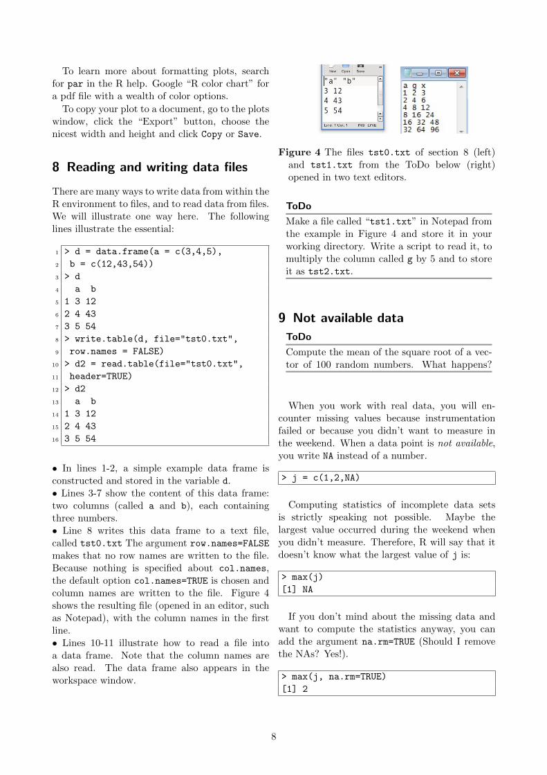
• In lines 1-2, a simple example data frame isconstructed and stored in the variable d.• Lines 3-7 show the content of this data frame:two columns (called a and b), each containingthree numbers.• Line 8 writes this data frame to a text file,called tst0.txt The argument row.names=FALSEmakes that no row names are written to the file.Because nothing is specified about col.names,the default option col.names=TRUE is chosen andcolumn names are written to the file. Figure 4shows the resulting file (opened in an editor, suchas Notepad), with the column names in the firstline.• Lines 10-11 illustrate how to read a file intoa data frame. Note that the column names arealso read. The data frame also appears in theworkspace window.

Figure 4 The files tst0.txt of section 8 (left)and tst1.txt from the ToDo below (right)opened in two text editors.

ToDo

Make a file called “tst1.txt” in Notepad fromthe example in Figure 4 and store it in yourworking directory. Write a script to read it, tomultiply the column called g by 5 and to storeit as tst2.txt.

9 Not available data

ToDo

Compute the mean of the square root of a vec-tor of 100 random numbers. What happens?

When you work with real data, you will en-counter missing values because instrumentationfailed or because you didn’t want to measure inthe weekend. When a data point is not available,you write NA instead of a number.

> j = c(1,2,NA)

Computing statistics of incomplete data setsis strictly speaking not possible. Maybe thelargest value occurred during the weekend whenyou didn’t measure. Therefore, R will say that itdoesn’t know what the largest value of j is:

> max(j)

[1] NA

If you don’t mind about the missing data andwant to compute the statistics anyway, you canadd the argument na.rm=TRUE (Should I removethe NAs? Yes!).

> max(j, na.rm=TRUE)

[1] 2

8

10 Classes

The exercises you did before were nearly all withnumbers. Sometimes you want to specify some-thing which is not a number, for example the nameof a measurement station or data file. In that caseyou want the variable to be a character string in-stead of a number.

An object in R can have several so-calledclasses. The most important three are numeric,character and POSIX (date-time combinations).You can ask R what class a certain variable is bytyping class(...).

10.1 Characters

To tell R that something is a character string, youshould type the text between apostrophes, other-wise R will start looking for a defined variable withthe same name:

> m = "apples"

> m

[1] "apples"

> n = pears

Error: object ‘pears’ not found

Of course, you cannot do computations withcharacter strings:

> m + 2

Error in m + 2 : non-numeric argument to

binary operator

10.2 Dates

Dates and times are complicated. R has to knowthat 3 o’clock comes after 2:59 and that Februaryhas 29 days in some years. The easiest way to tellR that something is a date-time combination iswith the function strptime:

1 > date1=strptime( c("20100225230000",

2 "20100226000000", "20100226010000"),

3 format="%Y%m%d%H%M%S")

4 > date1

5 [1] "2010-02-25 23:00:00"

6 [2] "2010-02-26 00:00:00"

7 [3] "2010-02-26 01:00:00"

• In lines 1-2 you create a vector with c(...).The numbers in the vectors are between apostro-phes because the function strptime needs char-acter strings as input.• In line 3 the argument format specifies how thecharacter string should be read. In this case theyear is denoted first (%Y), then the month (%m),day (%d), hour (%H), minute (%M) and second(%S). You don’t have to specify all of them, aslong as the format corresponds to the characterstring.

ToDo

Make a graph with on the x-axis: today, Sin-terklaas 2012 and your next birthday and onthe y-axis the amount of presents you expect oneach of these days. Tip: make two vectors first.

11 Programming tools

When you are building a larger program than inthe examples above or if you’re using someoneelse’s scripts, you may encounter some program-ming statements. In this Section we describe afew tips and tricks.

11.1 If-statement

The if-statement is used when certain computa-tions should only be done when a certain condi-tion is met (and maybe something else should bedone when the condition is not met). An example:

1 > w = 3

2 > if( w < 5 )

3 {

4 d=2

5 }else{

6 d=10

7 }

8 > d

9 2

• In line 2 a condition is specified: w should beless than 5.• If the condition is met, R will execute what isbetween the first brackets in line 4.• If the condition is not met, R will execute whatis between the second brackets, after the else inline 6. You can leave the else{...}-part out if

9

you don’t need it.• In this case, the condition is met and d has beenassigned the value 2 (lines 8-9).

To get a subset of points in a vector for whicha certain condition holds, you can use a shortermethod:

1 > a = c(1,2,3,4)

2 > b = c(5,6,7,8)

3 > f = a[b==5 | b==8]

4 > f

5 [1] 1 4

• In line 1 and 2 two vectors are made.• In line 3 you say that f is composed of thoseelements of vector a for which b equals 5 or b

equals 8.

Note the double = in the condition. Other con-ditions (also called logical or Boolean operators)are != ( 6=), <= (≤) and >= (≥). To test more thanone condition in one if-statement, use & if bothconditions have to be met (“and”) and | if one ofthe conditions has to be met (“or”).

11.2 For-loop

If you want to model a time series, you usually dothe computations for one time step and then forthe next and the next, etc. Because nobody wantsto type the same commands over and over again,these computations are automated in for-loops.

In a for-loop you specify what has to be doneand how many times. To tell “how many times”,you specify a so-called counter. An example:

1 > h = seq(from = 1, to = 8)

2 > s = c()

3 > for(i in 2:10)

4 {

5 s[i] = h[i] * 10

6 }

7 > s

8 [1] NA 20 30 40 50 60 70 80 NA NA

• First a vector is made.• In line 2 an empty vector is created. This isnecessary because when you introduce a variablewithin the for-loop, R will not remember it whenit has gotten out of the for-loop.• In line 3 the for-loop starts. In this case, i is

the counter and runs from 2 to 10.• Everything between the curly brackets (line 5) isprocessed 9 times. The first time i=2, the secondelement of h is multiplied with 10 and placed inthe second position of the vector s. The secondtime i=3, etc. The last two times elements of h

are requested that do not exist. Note that thesestatements are evaluated without any explicit er-ror messages.

ToDo

Make a vector from 1 to 100. Make a for-loopwhich runs through the whole vector. Multiplythe elements which are smaller than 5 and largerthan 90 with 10 and the other elements with 0.1.

11.3 Writing your own functions

Functions you program yourself work in the sameway as pre-programmed R functions.

1 > fun1 = function(arg1, arg2 )

2 {

3 w = arg1 ^ 2

4 return(arg2 + w)

5 }

6 > fun1(arg1 = 3, arg2 = 5)

7 [1] 14

8

• In line 1 the function name (fun1) and its argu-ments (arg1 and arg2) are defined.• Lines 2-5 specify what the function should do ifit is called. The return value (arg2+w) is shownon the screen.• In line 6 the function is called with arguments 3and 5.

ToDo

Write a function for the previous ToDo, sothat you can feed it any vector you like(as argument). Use the standard R func-tion length in the specification of the counter.

10

12 Some useful references

12.1 Functions

This is a subset of the functions explained in theR reference card.

Data creation• read.table: read a table from file. Arguments:header=TRUE: read first line as titles of thecolumns; sep=",": numbers are separated bycommas; skip=n: don’t read the first n lines.• write.table: write a table to file• c: paste numbers together to create a vector• array: create a vector, Arguments: dim: length• matrix: create a matrix, Arguments: ncol

and/or nrow: amount of rows/columns• data.frame: create a data frame• list: create a list• rbind and cbind: combine vectors into amatrix by row or column

Extracting data

• x[n]: the nth element• x[m:n]: the mth to nth element• x[c(k,m,n)]: specific elements• x[x>m & x<n]: elements between m and n

• x$n: element of list or data frame named n

• x[["n"]]: idem• [i,j]: element at ith row and jth column• [i, ]: row i

Information on variables• length: length of a vector• ncol or nrow: number of columns or rows in amatrix• class: class of a variable• names: names of objects in a list• print: show variable or character string on thescreen (used in scripts or for-loops)• return: show variable on the screen (used infunctions)• is.na: test if variable is NA

• as.numeric or as.character: change class tonumber or character string• strptime: change class from character todate-time (POSIX)

Statistics• sum: sum of a vector• mean: mean of a vector

• sd: standard deviation of a vector• rowSums (or rowMeans, colSums and colMeans):sums (or means) of all numbers in each row (orcolumn) of a matrix. The result is a vector.• max or min: largest or smallest element• range: min and max together• quantile(x,c(0.1,0.5)): sample the 0.1 and0.5th quantiles of vector x• cumsum: cumulative sum. Result is a vector.• lm(v1∼v2): linear fit (regression line) betweenvector v1 on the y-axis and v2 on the x-axis• nls(v1∼a+b*v2, start=ls(a=1,b=0)): non-linear fit. Should contain equation with variables(here v1 and v2 and parameters (here a and b)with starting values• coef: returns coefficients from a fit• summary: returns all results from a fit

Data processing• seq: create a vector with equal steps betweenthe numbers• rnorm: create a vector with random numberswith normal distribution (other distributions arealso available)• sort: sort elements in increasing order• t: transpose a matrix• aggregate(x,by=ls(y),FUN="mean"): splitdata set x into subsets (defined by y) and com-putes means of the subsets. Result: a new vector.• approx: interpolate. Argument: vector withNAs. Result: vector without NAs.• paste: paste character strings together• substr: extract part of a character string

Plotting• plot(x): plot x (y-axis) versus index number(x-axis) in a new window• plot(x,y): plot y (y-axis) versus x (x-axis) ina new window• image(x,y,z): plot z (x-axis, color scale)versus x (x-axis) and y (y-axis) in a new window• lines or points: add lines or points to aprevious plot• hist: plot histogram of the numbers in a vector• barplot: bar plot of vector or data frame• contour(x,y,z): contour plot• abline: draw line (segment). Arguments: a,b

for intercept a and slope b; or h=y for horizontalline at y; or v=x for vertical line at x.• curve: add function to plot. Needs to have an

11

x in the expression. Example: curve(x^2)• legend: add legend with given symbols (ltyor pch and col) and text (legend) at location(x="topright")• axis: add axis. Arguments: side (1=bottom,2=left, 3=top, 4=right)• mtext: add text on axis. Arguments: text

(character string) and side

• grid: add grid• par: plotting parameters to be specified beforethe plots. Arguments: e.g. mfrow(c(1,3)):amount of figures per page (1 row, 3 columns);new: add plot to previous plot - TRUE/FALSE

Plotting parametersThese can be added as arguments to plot, lines,image, etc. For help see par.• type: "l"=lines, "p"=points, etc.• col: color - "blue", "red", etc• lty: line type - 1=solid, 2=dashed, etc.• pch: point type - 1=circle, 2=triangle, etc.• main: title - character string• xlab and ylab: axis labels - character• log: logarithmic axis - "x", "y" or "xy"

Programming• function(arglist){expr}: function defini-tion: do expr with list of arguments arglist

• if(cond){expr1}else{expr2}: if-statement:if cond is true, then expr1, else expr2

• for(var in vec) {expr}: for-loop: thecounter var runs through the vector vec and doesexpr each run• while(cond){expr}: while-loop: while cond istrue, do expr each run

12.2 Keyboard shortcuts

There are several useful keyboard shortcuts forRStudio (see Help → Keyboard Shortcuts):• CRL+ENTER: send commands from script windowto command window• ↑ or ↓ in command window: previous or nextcommand• CTRL+1, CTRL+2, etc.: change between thewindows

Not R-specific, but very useful keyboard short-cuts:• CTRL+C, CTRL+X and CTRL+V: copy, cut and

paste• ALT+TAB: change to another program window• ↑, ↓, ← or →: move cursor• HOME or END: move cursor to begin or end of line• Page Up or Page Down: move cursor one pageup or down• SHIFT+↑/↓/←/→/HOME/END/PgUp/PgDn: selecttext

12.3 Error messages

• No such file or directory or Cannot

change working directory

Make sure the working directory and file namesare correct.• Object ‘x’ not found

The variable x has not been defined yet. Definex or write apostrophes if x should be a characterstring.• Argument ‘x’ is missing without default

You didn’t specify the compulsory argument x.• +R is still busy with something or you forgotclosing brackets. Wait, type } or ) or press ESC.• Unexpected ’)’ in ")" or Unexpected ’}’

in "}"

The opposite of the previous. You try to closesomething which hasn’t been opened yet. Addopening brackets.• Unexpected ‘else’ in "else"

Put the else of an if-statement on the same lineas the last bracket of the “then”-part: }else{.• Missing value where TRUE/FALSE needed

Something goes wrong in the condition-part(if(x==1)) of an if-statement. Is x NA?• The condition has length > 1 and only

the first element will be used

In the condition-part (if(x==1)) of an if-statement, a vector is compared with a scalar. Isx a vector? Did you mean x[i]?• Non-numeric argument to binary operator

You are trying to do computations with somethingwhich is not a number. Use class(...) to findout what went wrong or use as.numeric(...) totransform the variable to a number.• Argument is of length zero or Replacementis of length zero

The variable in question is NULL, which meansthat it is empty, for example created by c().Check the definition of the variable.

12