Toponym Resolution with Deep Neural Networks

Ricardo Jorge Barreira Custódio

Thesis to obtain the Master of Science Degree in

Telecommunications and Computer Engineering

Supervisors: Prof. Doutor Bruno Emanuel da Graça Martins

Prof. Miguel Daiyen Carvalho Won

Examination Committee

Chairperson: Prof. Doutor Luís Eduardo Teixeira RodriguesSupervisor: Prof. Doutor Bruno Emanuel da Graça Martins

Members of the Committee: Prof. Doutor David Martins de Matos

October 2017

Acknowledgements

First, I would like to thank Professor Bruno Emanuel da Graca Martins for his guidance

during this last and challenging year. His knowledge and constant motivation were a major

contribution to the work that we developed together.

Second, I would also like to thank my family, in particular my parents and my sister, for their

constant support and for giving me the opportunity to learn in such a distinguished institute as

Instituto Superior Tecnico.

Finally, I have to thank all my friends and colleagues for the constant support during

the hard, although also amazing, time spent at Instituto Superior Tecnico. A special word of

gratitude for my colleagues under the tutelage of Professor Bruno Martins, who went through

this last year experience with me. The countless hours we spent together, helping and making

fun of each other is something I will never forget. I share this achievement with you.

Ricardo Jorge Barreira Custodio

For my parents and sister,

Resumo

Resolucao de toponimos, i.e., inferir as coordenadas geograficas de uma string que representa

o nome de um local, e um problema fundamental no contexto de varias aplicacoes relacionadas

com extracao de informacao geografica e das ciencias de informacao geografica. O estado-da-

arte actual depende de regras heurısticas, combinadas com metodos de aprendizagem automatica

favorecendo metodos lineares simples. Esta dissertacao apresenta uma abordagem que favorece

Gated Recurrent Units (GRUs), um tipo de rede neuronal recorrente que pode ser utilizada

para modelar dados sequenciais, para construir representacoes das sequencias de palavras e

caracteres que correspondem as strings que serao associadas as suas respectivas coordenadas

geograficas. Estas representacoes sao posteriormente combinadas e passadas como input para

nos de feed-forward levando a sua previsao. O modelo pode ser treinado end-to-end com um

conjunto de ocurrencias de locais rotuladas, e.g., extraidas da Wikipedia. Esta dissertacao

apresenta os resultados de uma vasta avaliacao da performance do metodo proposto, usando

datasets de outros trabalhos na area. O modelo conseguiu alcancar resultados interessantes, por

vezes melhores do que alguns metodos do estado-da-arte de resolucao de toponimos.

Abstract

Toponym resolution, i.e. inferring the geographic coordinates of a given string that rep-

resents a placename, is a fundamental problem in the context of several applications related

to geographical information retrieval and to the geographical information sciences. The current

state-of-the-art relies on heuristic rules, together with machine learning methods leveraging sim-

ple linear methods. This dissertation advances an approach leveraging Gated Recurrent Units

(GRUs), a type of recurrent neural network architecture that can be used for modeling sequential

data, to build representations from the sequences of words and characters that correspond to the

strings that are to be associated with the coordinates, together with their usage context (i.e., the

surrounding words). These representations are then combined and passed to feed-forward nodes,

finally leading to a prediction decision. The entire model can be trained end-to-end with a set

of labeled placename occurrences, e.g., collected from Wikipedia. This dissertation presents the

results of a wide-ranging evaluation of the performance of the proposed method, using previous

works datasets. The model achieved some interesting results, sometimes even outperforming

state-of-the-art toponym resolution methods.

Palavras Chave

Keywords

Palavras Chave

resolucao de toponimos; redes neuronais; redes neuronais recorrentes; recuperacao de

informacao geografica

Keywords

toponym resolution; deep neural networks; recurrent neural networks; geographic

information retrieval

Contents

1 Introduction 1

1.1 Objectives . . . . . . . . . . . . . . . . . . . . . . . . . . . . . . . . . . . . . . . . 1

1.2 Methodology . . . . . . . . . . . . . . . . . . . . . . . . . . . . . . . . . . . . . . 2

1.3 Results and Contributions . . . . . . . . . . . . . . . . . . . . . . . . . . . . . . . 3

1.4 Dissertation Outline . . . . . . . . . . . . . . . . . . . . . . . . . . . . . . . . . . 3

2 Concepts and Related Work 5

2.1 Fundamental Concepts . . . . . . . . . . . . . . . . . . . . . . . . . . . . . . . . 5

2.1.1 Representing Textual Documents for Classification . . . . . . . . . . . . . 5

2.1.2 Naive Bayes Classifiers . . . . . . . . . . . . . . . . . . . . . . . . . . . . . 8

2.1.3 Discriminative Classifiers . . . . . . . . . . . . . . . . . . . . . . . . . . . 9

2.1.4 Convolutional Neural Network Classifiers . . . . . . . . . . . . . . . . . . 11

2.1.5 Recurrent Neural Network Classifiers . . . . . . . . . . . . . . . . . . . . . 12

2.2 Related Work . . . . . . . . . . . . . . . . . . . . . . . . . . . . . . . . . . . . . . 14

2.2.1 Toponym Recognition Methods . . . . . . . . . . . . . . . . . . . . . . . . 14

2.2.2 Heuristic Methods for Toponym Resolution . . . . . . . . . . . . . . . . . 15

2.2.3 Machine Learning Methods . . . . . . . . . . . . . . . . . . . . . . . . . . 20

2.2.4 Grid-Based Methods . . . . . . . . . . . . . . . . . . . . . . . . . . . . . . 24

2.3 Overview . . . . . . . . . . . . . . . . . . . . . . . . . . . . . . . . . . . . . . . . 28

3 Toponym Resolution Using a Deep Neural Network 29

3.1 The Proposed Approach . . . . . . . . . . . . . . . . . . . . . . . . . . . . . . . 29

3.2 Processing Input Data Using GRUs . . . . . . . . . . . . . . . . . . . . . . . . . 29

i

3.3 Predicting the Coordinates and Training the Network . . . . . . . . . . . . . . . 31

3.4 Summary . . . . . . . . . . . . . . . . . . . . . . . . . . . . . . . . . . . . . . . . 31

4 Experimental Evaluation 33

4.1 Datasets and Evaluation Metrics . . . . . . . . . . . . . . . . . . . . . . . . . . . 33

4.2 Experiments with Previous Works Datasets . . . . . . . . . . . . . . . . . . . . . 35

4.3 Experimental Results with Wikipedia Data . . . . . . . . . . . . . . . . . . . . . 37

4.4 Overview . . . . . . . . . . . . . . . . . . . . . . . . . . . . . . . . . . . . . . . . 38

5 Conclusions 41

5.1 Overview on the Contributions . . . . . . . . . . . . . . . . . . . . . . . . . . . . 41

5.2 Future Work . . . . . . . . . . . . . . . . . . . . . . . . . . . . . . . . . . . . . . 42

Bibliography 49

ii

List of Figures

2.1 Visualization generated with the t-SNE projection method for words close to the

word job from the embedding method proposed by Turian et al. (2010). . . . . . 6

2.2 CBoW and skip-gram model architectures . . . . . . . . . . . . . . . . . . . . . . 7

2.3 Graphical representation of the perceptron model. . . . . . . . . . . . . . . . . . 10

2.4 Graphical representation of an MLP . . . . . . . . . . . . . . . . . . . . . . . . . 10

2.5 Graphical representation of a convolutional neural network architecture with two

convolutional layers and a max-pooling layer. . . . . . . . . . . . . . . . . . . . . 12

2.6 Graphical representation of the processing done by a max-pooling node . . . . . 12

2.7 Graphical representation of a RNN. . . . . . . . . . . . . . . . . . . . . . . . . . 13

2.8 Illustration of a gated recurrent unit . . . . . . . . . . . . . . . . . . . . . . . . . 14

3.1 The neural network architecture proposed to address toponym resolution. . . . . 30

3.2 Detailed graphical representation of the GRUs bi-directional layers . . . . . . . . 31

4.1 Toponym distribution on the WOTR dataset . . . . . . . . . . . . . . . . . . . . 34

4.2 Toponym distribution on the Wikipedia dataset. . . . . . . . . . . . . . . . . . . 35

iii

iv

List of Tables

4.1 Detailed statistics of the datasets . . . . . . . . . . . . . . . . . . . . . . . . . . . 35

4.2 Experimental results obtained by the proposed method, compared with state-of-

the-art results . . . . . . . . . . . . . . . . . . . . . . . . . . . . . . . . . . . . . . 36

4.3 Experimental results obtained by the proposed method when trained with

Wikipedia data and evaluated on other datasets. . . . . . . . . . . . . . . . . . . 38

v

vi

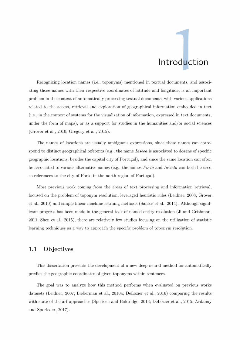
1IntroductionRecognizing location names (i.e., toponyms) mentioned in textual documents, and associ-

ating those names with their respective coordinates of latitude and longitude, is an important

problem in the context of automatically processing textual documents, with various applications

related to the access, retrieval and exploration of geographical information embedded in text

(i.e., in the context of systems for the visualization of information, expressed in text documents,

under the form of maps), or as a support for studies in the humanities and/or social sciences

(Grover et al., 2010; Gregory et al., 2015).

The names of locations are usually ambiguous expressions, since these names can corre-

spond to distinct geographical referents (e.g., the name Lisboa is associated to dozens of specific

geographic locations, besides the capital city of Portugal), and since the same location can often

be associated to various alternative names (e.g., the names Porto and Invicta can both be used

as references to the city of Porto in the north region of Portugal).

Most previous work coming from the areas of text processing and information retrieval,

focused on the problem of toponym resolution, leveraged heuristic rules (Leidner, 2008; Grover

et al., 2010) and simple linear machine learning methods (Santos et al., 2014). Although signif-

icant progress has been made in the general task of named entity resolution (Ji and Grishman,

2011; Shen et al., 2015), there are relatively few studies focusing on the utilization of statistic

learning techniques as a way to approach the specific problem of toponym resolution.

1.1 Objectives

This dissertation presents the development of a new deep neural method for automatically

predict the geographic coordinates of given toponyms within sentences.

The goal was to analyze how this method performs when evaluated on previous works

datasets (Leidner, 2007; Lieberman et al., 2010a; DeLozier et al., 2016) comparing the results

with state-of-the-art approaches (Speriosu and Baldridge, 2013; DeLozier et al., 2015; Ardanuy

and Sporleder, 2017).

Data collected from the latest dump of English Wikipedia1 articles collection, available from

Wikimedia Foundation2, was also employed to create a dataset to train the model. The final

goal was to assess if such training data would improve the overall method’s performance.

1.2 Methodology

The first stage of the work consisted on studying related work regarding similar toponym

resolution problems. This research gave particular attention to the machine learning approaches

chosen by the different authors on this task. Although there are many interesting previous

studies that have reported on high quality results, the absence of approaches based on modern

artificial neural networks suggested the opportunity to evaluate how deep learning methods

could be employed to predict geographic coordinates. Ideas from several previous publications,

addressing text classification problems and that have described innovative mechanisms based on

deep neural networks, were taken into consideration and subsequently incorporated in the final

network architecture that has been proposed.

After defining a deep neural network as the approach to the toponym resolution problem,

the technologies to use in this dissertation were considered. Due to its popularity and vast public

documentation, Python was the selected programming language to develop the project. Also,

the decision of using Python enabled the implementation of the deep neural network to rely on

Keras3 , a deep learning library that uses either Theano4 or TensorFlow5 as the computational

backend.

In order to train the deep neural network, previous works datasets were considered(Leidner,

2008; Lieberman et al., 2010a; DeLozier et al., 2016), plus a dataset created for the purpose of

this dissertation, containing data extracted from the English Wikipedia.

The predictive capability of the model was measured in terms of mean error distance, median

error distance and A@161(Leidner, 2008; Eisenstein et al., 2010; Wing and Baldridge, 2011;

Santos et al., 2014).

1https://en.wikipedia.org2https://dumps.wikimedia.org/3http://keras.io4http://deeplearning.net/software/theano/5http://www.tensorflow.org

2

1.3 Results and Contributions

The proposed architecture is the main contribution resulting from this dissertation. The

solution leverages a deep neural network, with parameters learned from training data (Schmid-

huber, 2015; LeCun et al., 2015; Goodfellow et al., 2016). The network uses bi-directional Gated

Recurrent Units (GRUs), a type of recurrent neural network architecture for modeling sequential

data, that was originally proposed by Chung et al. (2014) to build representations from the se-

quences of words and characters, that correspond to the strings that are to be associated with the

coordinates. These representations are then combined and passed to a sequence of feed-forward

nodes, finally leading to a prediction. The entire model can be trained end-to-end through the

back-propagation algorithm in conjunction with the Adam optimization method (Rumelhart

et al., 1988; Kingma and Ba, 2015), provided access to a training set of labeled sentences.

Three sets of experiments were considered, in an attempt to leverage how different training

data could affect the results. These correspond to:

• Experiments with the model trained with data from the same corpus used for evaluation;

• Experiments with the model trained with data from the Wikipedia and evaluated on

another corpus;

• Finally, experiments with a model trained with data from the Wikipedia, subsequently

adjusted with data from the same corpus used for evaluation.

The proposed model achieved interesting results in most of the experiments. In some cases,

state-of-the-art results were obtained in terms of mean error distance. One can therefore argue

that, deep neural networks such as the one developed in this dissertation, can be effective on

the difficult problem that is toponym resolution.

1.4 Dissertation Outline

This dissertation is organized as follows:

• Chapter 2 surveys important concepts and previous related work. First, an overview of

relevant topics (e.g., simple machine learning and deep neural networks) is made on Section

2.1. Then, a review of the approaches and techniques used in similar toponym resolution

tasks is presented in Section 2.2. The related work is divided in four categories: studies

3

focused on the task of recognizing toponyms; studies that leverage sets of heuristics to aid

toponym resolution; studies that leverage heuristics as features on simple linear machine

learning methods, and finally, studies focused on grid-based methods (i.e., divide the

Earth’s surface in a grid of cells and predict the cell that corresponds to a given toponym).

• Chapter 3 details the proposed approach, presenting the architecture of the deep neural

network that was considered for addressing toponym resolution.

• Chapter 4 presents the experimental evaluation of the proposed method. The chapter

starts by presenting the datasets used in the experiments, together with the experimental

methodology and evaluation metrics. Next, the chapter gives a detailed analysis of the

results obtained in the experiments.

• Chapter 5 outlines the main conclusions of this work, and it also presents possible devel-

opments for future work.

4

2Concepts and Related

Work

2.1 Fundamental Concepts

This section presents techniques related to modeling and classifying textual documents.

It begins with a subsection explaining how documents can be represented for computational

processing, and it then presents modern machine learning methods for building classifiers (Se-

bastiani, 2002; P. Murphy, 2012).

2.1.1 Representing Textual Documents for Classification

In order to perform computations with textual documents, one requires methods to prepro-

cess text data and transform it to structured data. One of those methods is the vector space

model (Salton et al., 1975). It is used for representing each document dj , from a given collec-

tion, as a vector containing one dimension per unique term from the vocabulary used within the

collection. This representation can be written formally as:

dj = (w1,j , w2,j , ..., wt,j) (2.1)

In the previous expression, wt,j represents the weight of a term t in the context of document

j. A term can be a single word or a phrase. The best way of determining these weights is by

using the numerical statistic known as the tf-idf (i.e., term frequency times inverse document

frequency) method, where each wt,j is given by the following equation:

wt,d = tft,d · log

(|D|

| {d′ ∈ D|t ∈ d′} |

)(2.2)

The tft,d component is the term frequency of term t in document d and is usually determined

as the number of times the term occurs in the document (i.e., raw frequency). The inverse

document frequency, given by log(

|D||{d′∈D|t∈d′}|

)determines how rare or common the term is

across all documents D. The component | {d′ ∈ D|t ∈ d′} | is the number of documents where

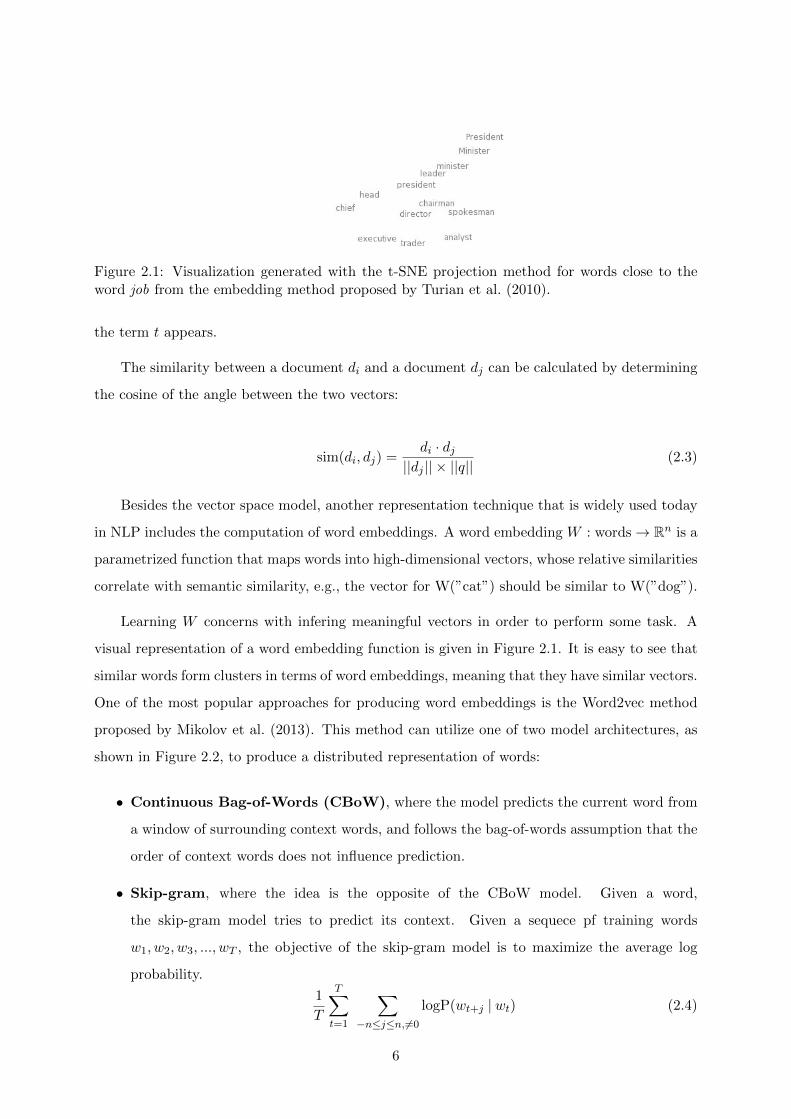
Figure 2.1: Visualization generated with the t-SNE projection method for words close to theword job from the embedding method proposed by Turian et al. (2010).

the term t appears.

The similarity between a document di and a document dj can be calculated by determining

the cosine of the angle between the two vectors:

sim(di, dj) =di · dj

||dj || × ||q||(2.3)

Besides the vector space model, another representation technique that is widely used today

in NLP includes the computation of word embeddings. A word embedding W : words→ Rn is a

parametrized function that maps words into high-dimensional vectors, whose relative similarities

correlate with semantic similarity, e.g., the vector for W(”cat”) should be similar to W(”dog”).

Learning W concerns with infering meaningful vectors in order to perform some task. A

visual representation of a word embedding function is given in Figure 2.1. It is easy to see that

similar words form clusters in terms of word embeddings, meaning that they have similar vectors.

One of the most popular approaches for producing word embeddings is the Word2vec method

proposed by Mikolov et al. (2013). This method can utilize one of two model architectures, as

shown in Figure 2.2, to produce a distributed representation of words:

• Continuous Bag-of-Words (CBoW), where the model predicts the current word from

a window of surrounding context words, and follows the bag-of-words assumption that the

order of context words does not influence prediction.

• Skip-gram, where the idea is the opposite of the CBoW model. Given a word,

the skip-gram model tries to predict its context. Given a sequece pf training words

w1, w2, w3, ..., wT , the objective of the skip-gram model is to maximize the average log

probability.

1

T

T∑t=1

∑−n≤j≤n, 6=0

logP(wt+j | wt) (2.4)

6

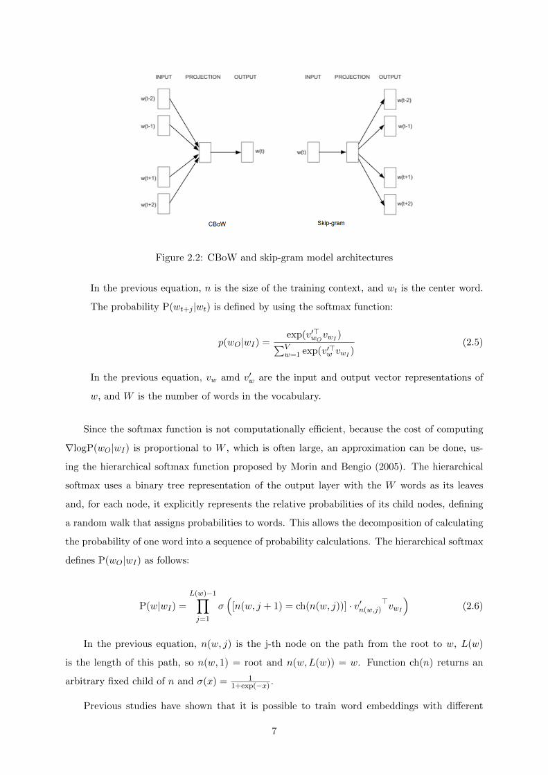
Figure 2.2: CBoW and skip-gram model architectures

In the previous equation, n is the size of the training context, and wt is the center word.

The probability P(wt+j |wt) is defined by using the softmax function:

p(wO|wI) =exp(v′>wO

vwI )∑Vw=1 exp(v′>w vwI )

(2.5)

In the previous equation, vw amd v′w are the input and output vector representations of

w, and W is the number of words in the vocabulary.

Since the softmax function is not computationally efficient, because the cost of computing

∇logP(wO|wI) is proportional to W , which is often large, an approximation can be done, us-

ing the hierarchical softmax function proposed by Morin and Bengio (2005). The hierarchical

softmax uses a binary tree representation of the output layer with the W words as its leaves

and, for each node, it explicitly represents the relative probabilities of its child nodes, defining

a random walk that assigns probabilities to words. This allows the decomposition of calculating

the probability of one word into a sequence of probability calculations. The hierarchical softmax

defines P(wO|wI) as follows:

P(w|wI) =

L(w)−1∏j=1

σ(

[n(w, j + 1) = ch(n(w, j))] · v′n(w,j)>vwI

)(2.6)

In the previous equation, n(w, j) is the j-th node on the path from the root to w, L(w)

is the length of this path, so n(w, 1) = root and n(w,L(w)) = w. Function ch(n) returns an

arbitrary fixed child of n and σ(x) = 11+exp(−x) .

Previous studies have shown that it is possible to train word embeddings with different

7

languages and produce a shared space where similar words from different languages are close

together (Zou et al., 2013; Ferreira et al., 2016).

For instance Hermann and Blunsom (2013) trained two models to produce sentence rep-

resentations of aligned sentences in two languages and use the distance between the sentence

representations as the learning objective. The authors minimize the following loss:

Edist(a, b) = ‖aroot − broot‖2 (2.7)

In the previous equation aroot and broot are the representations of two aligned sentences from

different languages. The authors compose aroot and broot as the sum of the embeddings of the

words in the corresponding sentence.

Concluding, word embeddings can be used as a way of computing similarities between terms,

or as representational basis for NLP tasks (e.g. text classification, named entity recognition,

entity linking, etc.).

2.1.2 Naive Bayes Classifiers

Naive Bayes classifiers are generative models based on Bayes’ theorem. Given two random

variables x and y, the theorem states that:

P(y|x) =P(x|y)× P(y)

P(x)(2.8)

The random variable y can represent the class we want to atribute to a given textual

document x. Naive Bayes classifiers explore the assumption that all the features describing the

document x are independent from each other in order to facilitate estimating P(x|y).

Because the denominator in Equation 2.8 is constant for all possible values of y, it can also

be ignored. To classify a document, the Naive Bayes classifier needs to determine the class with

the highest probability, according to:

y = arg maxk∈{1,...,k}

P(Ck)n∏i=1

P(xi|Ck) (2.9)

The component P(xi|Ck) is the probability of a term xi occurring in a document belonging

to a class Ck. This probability is determined in the training phase through a smoothed maximum

likelihood estimate (Lidstone, 1920; Juan and Ney, 2002), according to the following formula:

8

P(xi|Ck) =ni + 1

n+ |vocabulary|(2.10)

In the previous equation, ni is the total number of times the word xi appears in document

from class Ck, and n is the total number of words that the documents from class Ck have. The

|vocabulary| parameter corresponds to the number of different words in the document collection.

2.1.3 Discriminative Classifiers

Linear discriminative classifiers are a popular approach to address binary classification prob-

lems within NLP. These models receive a vector of input features x =< x1, ..., xn >, and they

consider that each input feature has an associated weight wj . The classifier computesn∑i=1

xiwi+b,

where b is a bias term, and then decides the output class with basis on the following activation

function:

y =

1 if

n∑i=1

xiwi + b ≥ 0

0 otherwise

(2.11)

The perceptron algorithm is one of the most frequently used methods for training linear

discriminative classifiers, operating in an on-line fashion (Rosenblatt, 1958). The weight of each

input feature is first initialized as a random value. At each iteration of the perceptron algorithm,

the weights are updated in the direction of correctly classifying the training instances, until the

classifier reaches a state where the following term is negligible.

∆wi = η(y − y)xi (2.12)

In the previous equation η is a learning rate (i.e., a constant value between 0.1 and 1). The

variable y is the class label and the y is the predicted class by the previous activation function.

Each time the perceptron fails to classify a training sample, it updates the weights, according

to:

wi := wi + ∆wi (2.13)

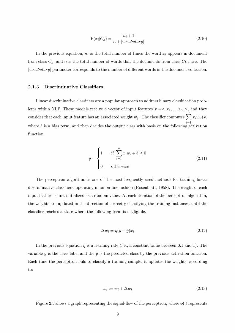
Figure 2.3 shows a graph representing the signal-flow of the perceptron, where φ(.) represents

9

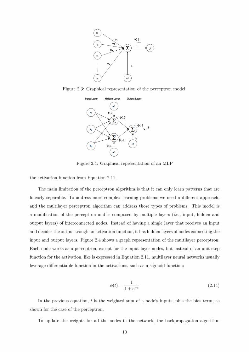
Figure 2.3: Graphical representation of the perceptron model.

Figure 2.4: Graphical representation of an MLP

the activation function from Equation 2.11.

The main limitation of the perceptron algorithm is that it can only learn patterns that are

linearly separable. To address more complex learning problems we need a different approach,

and the multilayer perceptron algorithm can address those types of problems. This model is

a modification of the perceptron and is composed by multiple layers (i.e., input, hidden and

output layers) of interconnected nodes. Instead of having a single layer that receives an input

and decides the output trough an activation function, it has hidden layers of nodes connecting the

input and output layers. Figure 2.4 shows a graph representation of the multilayer perceptron.

Each node works as a perceptron, except for the input layer nodes, but instead of an unit step

function for the activation, like is expressed in Equation 2.11, multilayer neural networks usually

leverage differentiable function in the activations, such as a sigmoid function:

φ(t) =1

1 + e−t(2.14)

In the previous equation, t is the weighted sum of a node’s inputs, plus the bias term, as

shown for the case of the perceptron.

To update the weights for all the nodes in the network, the backpropagation algorithm

10

(Lippmann, 1987) is used. If the output is an error, the algorithm back-propagates the error

trough the network, updating the weights. The output error of a node j can be given by:

ε(n) =1

2

∑j

(yj − yj)2 (2.15)

In the previous equation yj is the target value for the node j and y is the value produced by

the activation function of node j. The factor of 12 is conveniently added to cancel the exponent

when the error function is differentiated.

Finding the new updated weight wij value in each node is accomplished by using the

gradient-descent algorithm (Kelley, 1960). For each node, the following term is computed:

∆wi,j =∂ε(n)

∂wi,j(2.16)

In the previous equation, the parameter wi,j refers to the connection weight between j-th

node in a given layer and i-th node in the following layer. If the node is on the output layer of

the network, the previous equation is equivalent to the following:

∆wi,j = η(yi − yi)φ′(ti)yj (2.17)

For the nodes in inner layers, the multiple connections have to be taken into account. Let

wjk be the weight between k-th node in the previous layer (either inner or input layer) and j-th

node in the topmost hidden layer, the update is given by:

∆wi,j = η

(∑n

wnj(yn − yn)φ′(tn)

)φ′(tj)xk (2.18)

2.1.4 Convolutional Neural Network Classifiers

Convolutional neural networks (CNNs) are variations of multilayer perceptrons. They are

also trained trough backpropagation, but have a different architecture. A CNN uses copies of

the same neuron, making it easier to express computationally large models. Each neuron will

handle a subset of the input data and, together, these neurons will form a convolutional layer.

One can use as many convolutional layers in a network as it is necessary, depending on the

complexity of the classification or regression problem. Convolutional layers can be connected

11

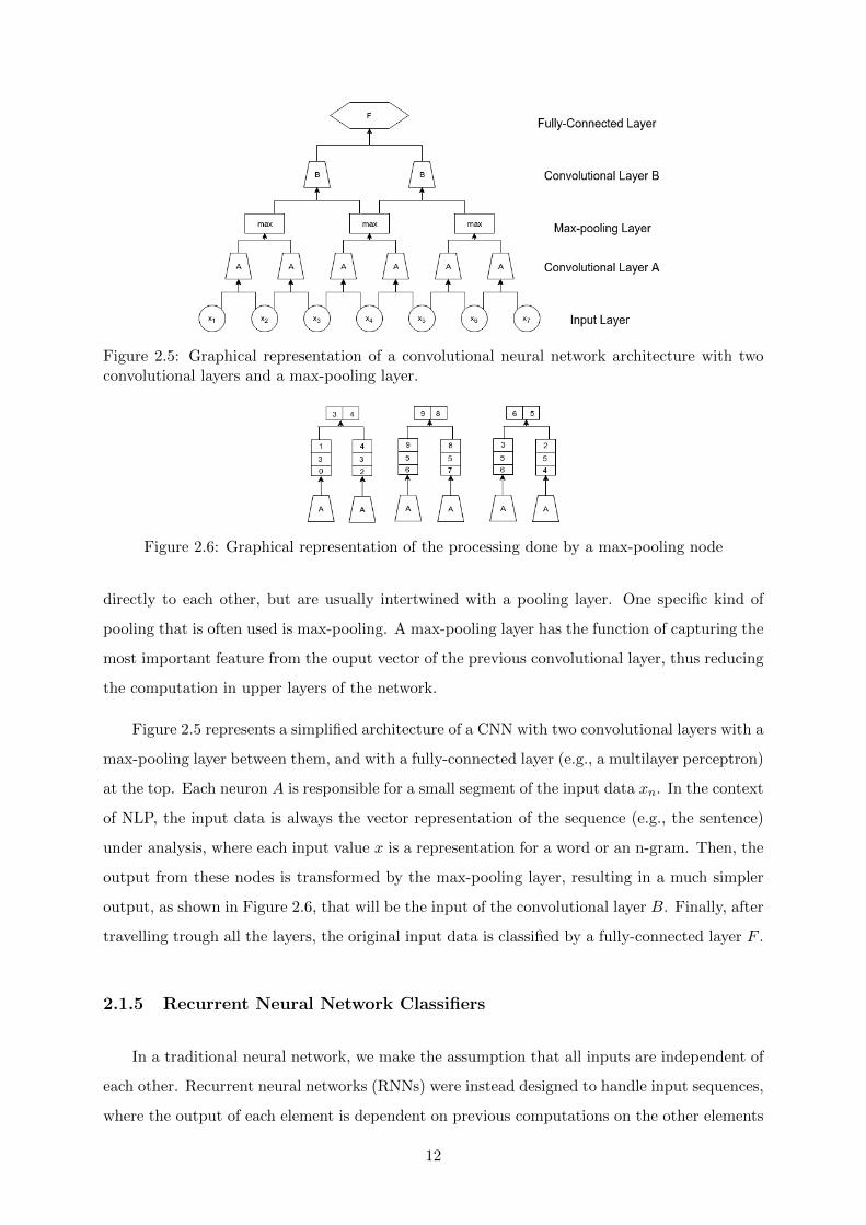
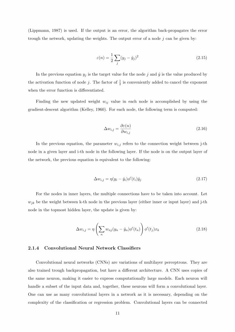
Figure 2.5: Graphical representation of a convolutional neural network architecture with twoconvolutional layers and a max-pooling layer.

Figure 2.6: Graphical representation of the processing done by a max-pooling node

directly to each other, but are usually intertwined with a pooling layer. One specific kind of

pooling that is often used is max-pooling. A max-pooling layer has the function of capturing the

most important feature from the ouput vector of the previous convolutional layer, thus reducing

the computation in upper layers of the network.

Figure 2.5 represents a simplified architecture of a CNN with two convolutional layers with a

max-pooling layer between them, and with a fully-connected layer (e.g., a multilayer perceptron)

at the top. Each neuron A is responsible for a small segment of the input data xn. In the context

of NLP, the input data is always the vector representation of the sequence (e.g., the sentence)

under analysis, where each input value x is a representation for a word or an n-gram. Then, the

output from these nodes is transformed by the max-pooling layer, resulting in a much simpler

output, as shown in Figure 2.6, that will be the input of the convolutional layer B. Finally, after

travelling trough all the layers, the original input data is classified by a fully-connected layer F .

2.1.5 Recurrent Neural Network Classifiers

In a traditional neural network, we make the assumption that all inputs are independent of

each other. Recurrent neural networks (RNNs) were instead designed to handle input sequences,

where the output of each element is dependent on previous computations on the other elements

12

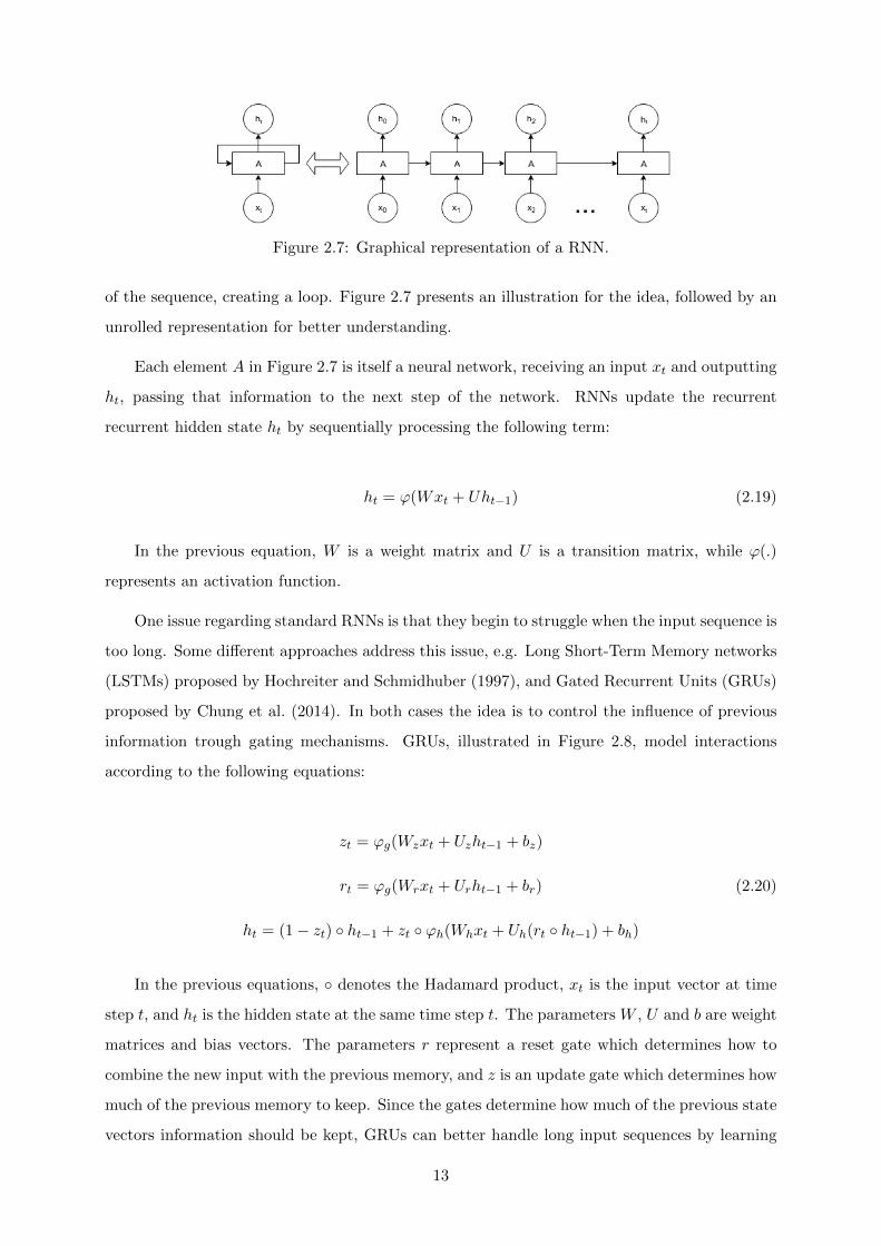
Figure 2.7: Graphical representation of a RNN.

of the sequence, creating a loop. Figure 2.7 presents an illustration for the idea, followed by an

unrolled representation for better understanding.

Each element A in Figure 2.7 is itself a neural network, receiving an input xt and outputting

ht, passing that information to the next step of the network. RNNs update the recurrent

recurrent hidden state ht by sequentially processing the following term:

ht = ϕ(Wxt + Uht−1) (2.19)

In the previous equation, W is a weight matrix and U is a transition matrix, while ϕ(.)

represents an activation function.

One issue regarding standard RNNs is that they begin to struggle when the input sequence is

too long. Some different approaches address this issue, e.g. Long Short-Term Memory networks

(LSTMs) proposed by Hochreiter and Schmidhuber (1997), and Gated Recurrent Units (GRUs)

proposed by Chung et al. (2014). In both cases the idea is to control the influence of previous

information trough gating mechanisms. GRUs, illustrated in Figure 2.8, model interactions

according to the following equations:

zt = ϕg(Wzxt + Uzht−1 + bz)

rt = ϕg(Wrxt + Urht−1 + br) (2.20)

ht = (1− zt) ◦ ht−1 + zt ◦ ϕh(Whxt + Uh(rt ◦ ht−1) + bh)

In the previous equations, ◦ denotes the Hadamard product, xt is the input vector at time

step t, and ht is the hidden state at the same time step t. The parameters W , U and b are weight

matrices and bias vectors. The parameters r represent a reset gate which determines how to

combine the new input with the previous memory, and z is an update gate which determines how

much of the previous memory to keep. Since the gates determine how much of the previous state

vectors information should be kept, GRUs can better handle long input sequences by learning

13

Figure 2.8: Illustration of a gated recurrent unit

how the internal memory should behave.

2.2 Related Work

This section overviews important related work in the area of toponym resolution. Previous

publications are divided into toponym recognition methods, heuristic methods, machine learning

methods, and grid-based methods.

2.2.1 Toponym Recognition Methods

Toponym recognition is the specific named entity recognition (NER) subtask of finding

all textual references to geographic locations (i.e., toponyms), that precedes every toponym

resolution method. The task can be addressed by standard NER methods (Al-Rfou et al., 2015;

Finkel et al., 2005).

Given the low recall in standard NER systems, Lieberman and Samet (2011) saw the need

for a comprehensive, multifaceted toponym recognition method designed for streaming news.

This method is divided in two stages. In the first stage the authors generated a dictionary of

possible entities using many sources of evidence. In the second stage, the aim was trying to

resolve entity types using post-processing filters.

The entities in the dictionary are extracted from the document’s text through gazetteer

matching, parts-of-speech (POS) tagging, and standard NER techniques. The results contain

not only locations but also proper nouns and cue words. Cue words are useful for resolving

geo/non-geo ambiguities, and these include words like county (geo) and professor (non-geo).

14

After finding the entities, a series of post-processing filters are applied, according to the

following order:

• Toponym refactoring: The aim of this filter is to address the issue of the same location

being referred in different ways, depending on who is writing it. For example, the word

county can be written before or after the location name, or it can be even abbreviated as

co..

• Active verbs: This filter distinguishes toponyms from non-toponyms based on the idea

that locations tend to be passive, i.e. they do not perform actions. An entity followed by

an active verb will be disqualified from being a toponym.

• Noun adjuncts: This filter finds entities that function has adjectives by modifying other

nearby nouns. For example in the sentence U.S. officials, the name U.S. is a noun adjunct,

and therefore it will not be qualified as a toponym by this filter.

• Type propagation: This filter addresses the issue that entities found using the POS tagger

have an unknown type, whilst entities found using the NER system have specific types.

Type propagation within each group will make the types consistent.

The authors incorporated their methods into the NewsStand system (Teitler et al., 2008) and

compared them with the toponym recognition methods of OpenCalais1 and Yahoo! Placemaker2

on two different corpora: LGL (Lieberman et al., 2010a) and Clust, which is a corpus created by

Lieberman and Samet (2011), composed by clusters of news articles obtained from NewsStand.

Their methods achieved high values for toponym recall, outperforming the competitors, and

showed very consistent results when tested with weekly samples of articles, which means it is

well suited for streaming news.

2.2.2 Heuristic Methods for Toponym Resolution

Most previous work in the area follows the idea that, given a document with identified

toponyms, a series of pre-defined rules can be used over each toponym to determine which

location it corresponds to. These rules usually rely on gazetteers, which are dictionaries for

locations (e.g., Geonames or the Getty Thesaurus) that contain several metadata fields in each

1http://opencalais.com2http://developer.yahoo.com/geo/placemaker

15

entry (e.g., population, area, administration level, etc.). Occasionally, gazetteers are specifically

created by the authors for the context of their toponym resolution work.

Leidner (2007) applied several heuristics in his toponym resolution method, considering a

particular ordering. Those heuristics were:

• Resolve unambiguous, when there’s only one candidate location for a given toponym,

this heuristic simply assign that location.

• ”Contained-in” qualifier following, match patterns that resolve some toponyms based

on local context (e.g. Oxford, England, UK).

• Superordinate mention, applied on the state, country and continent levels, that dis-

ambiguate toponyms according to the following example: A mention of Tennessee in the

same document where the resolution of Memphis is attempted, triggers the interpretation

Memphis, TN, USA.

• Largest population, assigns the referent with the largest population size, given by an

authority list.

• One-referent-per-discourse, is inspired on the work of Gale et al. (1992), and it as-

sumes that a place name mentioned in a discourse refers to the same location throughout

the discourse, i.e., a resolved toponym can be seen to propagate its interpretation to other

instances of the same toponym in the same discourse or discourse segment (e.g., ...Lon-

don...London,UK...London... all refer to the city of London, capital of England)

• Spatial minimality, assumes that, the smallest region that is able to ground a whole set

of toponyms mentioned in some span of text is the one that gives them their interpretation.

• Textual distance to unambiguous neighbors (in tokens), for a given ambiguous

toponym t, considers the surrounding unambiguous toponyms and assign the referent

which is geographically the closest to all of them as the interpretation for t.

• Discard off-threshold, computes the geographic focus (centroid) for the toponyms men-

tioned in the document, and eliminate all candidate referents that are more than 2 standard

deviations away from it.

• Frequency weighting, gives higher importance to more frequent toponyms in a text.

• Prefer higher-level referents, resolves a toponym to the candidate referent that has

the higher-level of importance in a hierarchy, such as countries over cities, or continents

16

over countries (e.g., Africa is assigned to the continent Africa rather than the cities Africa,

Mexico, Africa, IN., or Africa, OH, USA).

Lieberman et al. (2009) addressed the issue of toponym resolution in spreadsheets via spatial

coherence, i.e, cells with spatial data that are nearby in the spreadsheet contain data that

share spatial characteristics in the real world. The strategy implemented for recognizing spatial

cells employed several heuristic methods modeled after place recognition techniques for natural

language text (Amitay et al., 2004). The authors used the Geonames gazetteer for candidate

extraction and, in addition, they perform a search for cue-words, prominent places, and political

regions, as well as textually-specified hierarchies. To recognize addresses, the authors used the

Yahoo! address geocoding API3.

To disambiguate the resulting cells with multiple gazetteer candidate locations and other

types of spatial data assigned to them, the authors noted that data in spreadsheets is usually

organized so that each data record corresponds to a row in the spreadsheet, and each data

attribute, spatial or non-spatial, corresponds to a column. Therefore, the first step of their

resolving methodology is classifying every column in the spreadsheet as spatial or non-spatial,

and assigning a spatial data type to respective columns, which will be useful for filtering the

gazetteer records assigned to the cells in each column. In the second step, the authors noted that

when a spreadsheet contains multiple spatial columns, they usually tend to exhibit a containment

relationship (e.g. Paris, Texas, USA each in the same row within different columns).

Comma groups refer to lists of toponyms found in documents, separated by some sort of

token (e.g. ”and”, ”or”, ”,”, etc.). The motivation for understanding comma groups within the

context of toponym resolution is that, usually, toponyms in comma groups share some kind of

attribute with each other. For example, in the comma group Rome, Paris, Berlin and Brussels

all the toponyms share a common thread of large, prominent capital cities. Lieberman et al.

(2010b) presented three heuristics to identify these common threads and therefore resolve comma

groups:

• Prominence: Checks if all toponyms in the group have a prominent location interpretation

(i.e. population ≥ 100k) and, if so, resolve the toponyms in the group accordingly.

• Proximity: Uses an iterative method to measure the distances between all possible in-

terpretations for every toponym and chooses the resulting group that minimizes those

3http://developer.yahoo.com/

17

distances. The authors determined that for this heuristic, two locations are close to each

other if the distance between them is less than 50 miles.

• Sibling: Checks if all toponyms in the group share a parent in a geographical hierarchy,

e.g. states in the same country, counties in the same state, etc.

To evaluate their method, the authors implemented these heuristics in a geotagger and

measured how often they were used and the precision of their method when resolving comma

groups. To perform their experiments, the authors created a dataset of news articles extracted

from the NewsStand system (Teitler et al., 2008). A comma group was considered correct if all

its toponyms were recognized and resolved correctly. The overall precision of the heuristics used

was about 95% or higher, indicating that inferring common threads of comma groups can be a

source of highly accurate evidence for geotagging toponyms. From the heuristic usage statistics

it is also easy to conclude that sibling (49%) and prominence (39%) play an important role in

recognizing and resolving comma groups.

Lieberman et al. (2010a) proposed that understanding local lexicons in news documents can

be relevant when disambiguating toponyms. The key premise is that for readers in different

places, the same placename can refer to different locations. For example, a Texas reader might

identify Paris as Paris, Texas rather than Paris, France, which is more prominent but less

relevant in the reader’s local lexicon. To automatically infer a local lexicon, the authors analyze

toponyms in a collection of articles from a news source and determine a convex hull of the

geographic coordinates of the toponyms extracted. This local lexicon is then used as one of

the heuristics in their toponym resolution method, by computing the geographic centroid of the

source’s inferred local lexicon and resolving toponyms that are geographically proximate to the

centroid. The authors concluded that this heuristic is irrelevant when the corpus is composed

by articles with more prominent toponyms (e.g. the ACE 2005 English SpatialML corpus (Mani

et al., 2008)) but is specially effective when the corpus is composed by articles from smaller and

geographically-constrained newspapers, namely in the LGL (Local-Global Lexicon) corpus, which

is a dataset created by the authors that consists of news articles extracted from the NewsStand

system.

To evaluate their toponym resolution method, the authors used precision and recall mea-

sures. Using a toponym oracle that ensures perfect toponym recognition, their method achieved

a precision of 0.968 and recall of 0.890 in the ACE SpatialML corpus, and a precision of 0.964

and recall 0.817 on the LGL corpus, outperforming the baseline methods implemented for the

experiments. Those methods were inspired in methods from MetaCarta (Rauch et al., 2003),

18

Web-a-Where (Amitay et al., 2004) and a system developed by Volz et al. (2007).

Grover et al. (2010) integrated an heuristic georesolution method for into two distinct

projects, namely GeoDigRef and Embedding GeoCrosswalk to address the problem of georefer-

encing digitized historical collections. The georesolution method consists in two main stages.

In the first stage, named gazetteer place names lookup, duplicate place names that were

previously recognized are reduced to a single representative. The place names are then passed

to a gazetteer lookup script, which outputs the candidates for each place name extracted from

either Geonames or the Ordnance Survey-derived GeoCrossWalk gazetteer, along with their

respective geospatial coordinates and other features related to the candidate.

The second stage, i.e., the resolution stage, takes the output from the lookup and applies

heuristics in order to rank the candidate entries. The heuristics used by the authors were as

follows:

• Feature type: Leverages populated places to facilities (e.g., buildings).

• Population: Gives preference to more populated places, and the authors found out this

heuristic is particularly relevant in newspaper text.

• Contextual information: Looks for containment and proximity information to favour can-

didates (e.g., the containment relation in Leith, Edimburg).

• A locality parameter from the user: The georesolver cam be called with a parameter that

specifies the geographic focus of a document as a latitude, longitude and radius.

• Clustering: Follows the intuition that many of the places in a document are close to each

other. For each candidate for a place name, the authors compute its distance from the

nearest candidate for each other place names in the same document. Candidates with

smaller average distance to the nearest five other places are preferred.

The authors scaled the value for each heuristic to be in the range 0-1, using logarithmic

scaling for the population and clustering. The scaled values are combined to produce a single

score for each candidate. In the GeoDigRef project, the authors worked with two collections,

namely, the Online Historical Population Reports for Britain and Ireland from 1801 to 1937

(Histpop4), and the Journals of the House of Lords (1688 to 1854) from the BOPCRIS 18th

4http://www.histpop.org.uk/

19

Century Parliamentary Publications BOPCRIS5. In the Embedding GeoCrosswalk project, the

authors worked with the Stormont Papers6, which are 84 volumes of parliamentary debates from

the start of the Northern Irish Parliament from 1921 to 1972.

To create the test data, the authors hand annotated the correct interpretation for each place

name. For Histpop and BOPCRIS, they did it twice, once using the GeoCrossWalk gazetteer

and a second time using Geonames. For Stormont, the authors only used Geonames because

the GeoCrossWalk gazetteer does not cover Northern Ireland. Two kinds of comparisons were

considered: strict matching, where hand annotated and system choices should be identical, and

within 5 km matching, where each hand annotation and a candidate would be counted the

same if their grid references were within 5 km of each other. The authors also tested the effect

that the locality parameter heuristic had on the results of their method, turning it on and off.

Given that the evaluation corpora contains mainly locations in the United Kingdom, the input

of the locality parameter corresponded to that specific region. The results show significant

improvement when this heuristic is considered, mainly in the Geonames gazetteer, given the

fact that this gazetteer outputs more worldwide candidates than the GeoCrossWalk gazetteer,

where the locality parameter heuristic becomes a bit redundant.

2.2.3 Machine Learning Methods

Another approach to resolve toponyms includes using heuristics, such as those from the

previous section, as features in machine learning algorithms.

Lieberman and Samet (2012) addressed the use of adaptive context features in geotagging

algorithms for streaming news. Those adaptive context features are based on computing features

within a window of context around each toponym.

The framework used by the authors to test their adaptive context features was originally

developed for and is an integral component of the NewsStand (Teitler et al., 2008) and Twit-

terStand (Sankaranarayanan et al., 2009) systems. The toponym resolution method assigns a

decision on whether for a given toponym/interpretation pair (t, lt), the disambiguation candi-

dates lt are drawn from a gazetteer, is a correct or incorrect disambiguation. To this purpose,

random forests (Breiman, 2001) were used for classifying each pair, according to descriptive

features. This method constructs many decision trees based on different random subsets of the

dataset, sampled with replacement. Each decision tree is constructed using random subsets of

5http://www.parl18c.soton.ac.uk6http://stormontpapers.ahds.ac.uk

20

features from the training feature vectors. To classify a new feature vector, each tree in the

forest votes for the vector’s class, and the consensus is taken as the result.

The authors considered several baseline toponym resolution features in their methods,

namely:

• Number of interpretations for toponym t.

• The population of lt, where a larger population indicates that lt is more well-known, and

should thus perhaps be preferred.

• Number of alternate names for lt in various languages. More names also indicates that lt,

is more well-known.

• Geographic distance between lt and an interpretation of a dateline toponym (i.e., toponym

in the dateline of the news article), which establishes a general location context for a news

article.

• Geographic distance between lt and the newspaper’s local lexicon (Lieberman et al., 2010a),

which encodes the expected location of its primary audience, expressed as a lat/long point.

Adaptive context features reflect two aspects of toponym coocurrence, and also the evidence

that interpretations for different toponyms bring to each other:

• Proximate interpretations features are based on geographic distance. To compute

them, for each other toponym o in the context window around t, the closest interpretation

lo to lt is found. Then, the average of the geographic distances to the other interpretations

is calculated. The learning procedure can learn appropriate distance thresholds from its

training data.

• Sibling interpretations features capture the relationships between textually proximate

toponyms that share the same country, state, or other administrative division. For each

toponym/interpretation pair (t, lt), sibling features value the number of other toponyms o

in the window around t with an interpretation that is a sibling of lt at a given resolution.

These two classes of interpretation relationships are captured and encoded in features. When

computing these features, two variables are taken into account:

• Window breadth: size of the window around t (i.e., controls how many toponyms around

t are to be used in aiding its resolution).

21

• Window depth: maximum number of interpretations to be considered for each toponym in

the window. These interpretations are ranked using various factors, namely, the number

of alternate names for the location in other languages, population of the location, or

geographic distance.

In the experiments, the adaptive method was put in competition against other geotagging

methods, namely Thomson Reuter’s OpenCalais 7 and Yahho!’s Placemaker8. Three different

datasets were used in the tests, namely ACE SpatialML, LGL and CLUST. A given interpreta-

tion is considered correct if the geographic distance between its geospatial coordinates and the

ground truth coordinates lies within a threshold of 10 miles. The adaptive method has the best

overall precision, especially for the LGL and CLUST datasets, proving that adaptive context

features can be a flexible and useful addition to geotagging algorithms.

Santos et al. (2014) addressed the problem of toponym resolution by first identifying to-

ponyms using Standford’s NER system, and then ranking the candidates through a procedure

inspired on previous work in entity linking, which involves the following steps:

Query expansion: Given a reference, expansion techniques are apllied to try to identify

other names in the source document that reference the same entity. For example, NY is a

reference for New York and US for United Sates.

Candidate generation: This step looks for similar entries as the query in a gazetteer built

from Wikipedia and returns the top 50 most likely entries, according to an n-gram retrieval model

supported by a Lucene9 index. The gazetteer is based on English Wikipedia10 subset containing

all the geotagged pages, plus all pages categorized in DBPedia11 as corresponding to either

persons, organizations and locations.

Candidate ranking: The LambdaMART learning to rank algorithm (Burges, 2010), as

implemented in the RankLib12 library, is used to sort the retrieved candidates according to the

likelihood of begin the correct referent. The ranking model leverages on a total of 58 different

ranking features for representing each candidate. These features vary from authority features

(e.g., the PageRank score of the candidate, computed over Wikipedia’s link graph) to textual

similarity (e.g., cosine similarity between tf-idf representations for the query document and for

7http://opencalais.com8http://developer.yahoo.com/geo/placemaker9http://lucene.apache.org/index.html

10https://dumps.wikimedia.org/index.html11http://dbpedia.org/index.html12http://people.cs.umass.edu/ vdang/ranklib.html

22

the candidate’s textual description in Wikipedia), including also geographical features. The

geographical features are particularly important given the purpose of toponym resolution, and

the ones used by the authors were the following:

• Number of times that the candidate appears also as a disambiguation candidate for other

place references in the same document, or in a window of 50 tokens surrounding the

reference.

• Number of inhabitants of a given candidate place.

• Area of the region corresponding to the candidate place in squared kilometers.

• Number of place references that are shared by both the query’s source text and the can-

didate’s textual description from Wikipedia.

• Jaccard similarity coefficient, computed between the set of place references occurring in the

query document, and the set of place references from the candidate’s textual description.

• Number of place references in the source text that are not mentioned in the candidate’s

textual description from Wikipedia.

• Geospatial distance between the coordinates of the document, assigned by an automated

document geocoding method based on min-hash and locality sensitive hashing (Broder,

1997), and the candidate’s coordinates, using the geodetic formulae from Vincenty (1975).

• Geospatial containment, i.e., assigning the entire contents of the query document to a

geospatial region defined over the surface of the Earth, and then verifying if the candidate’s

coordinates are contained within that region.

• Mean and minimum geospatial distance between the candidate disambiguation, and the

best candidate disambiguations for other place references in the same document.

• Geospatial distance between the candidate disambiguation, and the best candidate for the

place reference that appears closer in the same query document.

• Area of the convex hull and of the concave hull obtained from the geospatial coordinates

of the candidate disambiguation and the best candidates for other place references made

in the same document.

Candidate validation: It may be the case that the correct referent is not given in the

gazetteer, this step decides if the top ranked referent is an error, trough a random forest classifier

23

that reuses the features from the previous step, and considers additional features for representing

the top ranked referent, such as the candidate ranking score, or the results from well known

outlier detection tests, that try to see if the top ranked candidate is significantly different from

the others.

To evaluate their approach, besides Wikipedia documents, the authors also used the local-

global lexicon (LGL) dataset (Lieberman et al., 2010a) and the ACE SpatialML dataset (Mani

et al., 2008). The authors compared two different configurations of the proposed place reference

disambiguation approach, namely one configuration corresponding to a standard name entity

disambiguation setting, without geographic features and another introducing the usage of the ge-

ographic features they proposed in their work. The authors used the geospatial distance between

the coordinates returned as the disambiguation, and the correct geospatial coordinates, as the

main evaluation metric. The results show that although not having significant improvements,

the system’s performance benefits from the introduction of the geographic features.

Similarly to Santos et al. (2014), Ardanuy and Sporleder (2017) proposed a weakly-

supervised method named GeoSem that combines the strengths of previous work on toponym

resolution and entity linking, by exploiting both geographic and semantic features. The au-

thors start by building a knowledge base of locations, composed by georeferenced articles from

Wikipedia complemented with information from Geonames. Each location has a list of alterna-

tive names, selected geographic features (e.g., latitude, longitude, population and the country

where the location is situated) and semantic features (e.g. context of words extracted from parts

of the body of the Wikipedia article). Leveraging the knowledge base, the authors attempt to

select the right candidate location with the given toponym. Their method distinguishes be-

tween local features (i.e., features that measure the compatibility of a candidate location with

the referent of a toponym in a text without regard to compatibility with co-occurring toponyms)

and global features (i.e., features that take into account the interdependence between entities

to measure the compatibility of a candidate), taking inspiration on previous work by Han et al.

(2011). The local and global features are then combined and fed into the method, that decides

which is the most likely candidate for a given toponym.

2.2.4 Grid-Based Methods

Grid-based toponym resolution methods, divide the Earth’s surface in a grid of cells and

classify toponyms according to which cell they belong to.

24

Speriosu and Baldridge (2013) proposed 3 different grid-based toponym resolvers, namely

TRIPD, WISTR and TRAWL.

TRIPDL is an acronym for Toponym Resolution Informed by Predicted Document Loca-

tions and this method divides the Earth’s surface according to a 1Ao by 1Ao grid of cells, and

then learns language models for each cell from Wikipedia geolocated articles (i.e., from a col-

lection of Wikipedia pages refered to as the GeoWiki dataset). It then computes the similarity

between a document d, represented as a distribution over words, against each cell, and chooses

the closest one, using the Kullback-Lieber (KL) divergence (Kullback and Leibler, 1951). Then,

the authors normalize the values of the KL-divergence to obtain a probability P(c|d) that is used

for all toponyms t in d to define the following distribution:

PDL(l|t, d) =P(cl|d)∑

t′∈G(t) P(ct′ |d)(2.21)

In the previous equation, G(t) is the set of the locations l for toponym t in the Geonames

gazetteer, and cl is the cell that contains l. To disambiguate a toponym, TRIPDL chooses the

location that maximizes P(c|d).

WISTR is an acronym for Wikipedia Indirectly Supervised Toponym Resolve, and this

method extracts training instances automatically from the Geowiki dataset to learn text clas-

sifiers. It begins by detecting toponyms in Geowiki using the OpenNLP NER13 system. Then,

for each toponym, it gets all candidate locations from the geonames gazetteer. The candidate

location that is closest to the Wikipedia article’s location is used as the label for the training

instance. Context windows of twenty words w to each side of each toponym are used as features.

After all the relevant instances are extracted, they are used to train logistic regression classifiers

P(l|t, w) for location l and toponym t. The location that maximizes this probability is chosen

to disambiguate a new toponym.

TRAWL is an acronym for Toponym Resolution via Administrative levels and Wikipedia

Locations and this last approach corresponds to a hybrid of TRIPDL and WISTR that gives

preference to locations more administratively prominent. This means that, for example, if a

country and a city have the same name, the method will give preference to the country. TRAWL

selects the optimal candidate location l according to:

l = arg maxlP (al|t)(λtP (l|t, ct) + (1− λt)PDL(l|t, d) (2.22)

13http://opennlp.apache.org

25

In the previous equation, P(al|t) is the administrative level component and is given by the

fraction of the representative points of location l and representative points for all locations l ∈ t.

All cities have only one representative point in geonames, so this will give higher probability to

states and countries because they contain usually thousands of points. The rest of the Equation

2.22 is a linear combination of WISTR and TRIPDL. Since the authors are more confident that

WISTR will give the right prediction, they assign a weight λt to the local context distribution

that is given by:

λt =f(t)

f(t) + C(2.23)

In the previous equation, f(t) is the fraction of training instances for toponym t of all

instances extracted from Geowiki, while the constant C is set experimentally.

To evaluate the results, the authors used yet another resolver (i.e., a method named Spatial

Prominence via Iterative Distance Evaluation and Reweighting, with the acronym SPIDER)

as a baseline. SPIDER assumes that toponyms in the same document tend to refer to nearby

locations and gives preference to more prominent locations (i.e. locations that tend to get se-

lected more often in a corpus). The authors also used two simpler baseline resolvers: RANDOM

(i.e., randomly select a location in the candidate locations) and POPULATION (i.e., select the

candidate location with the highest population).

To evaluate the different resolvers, the authors computed the mean and median of the

distance between the correct and predicted locations for each toponym. Precision and recall

were also used when dealing with NER-identified toponyms. The authors used the TR-CoNLL

(i.e., articles about international events, used primarily in the CoNLL-02 competition on NER)

and CWar (collection of documents about the American Civil War14) corpora to support their

experiments.

The authors concluded that their resolvers outperformed standard minimality resolvers.

Overall, the resolver with the best results, both in accuracy, precision and recall, was the WISTR

resolver, although in the CWar corpus this method had to be combined with SPIDER to achieve

a better accuracy.

To address the dependency on gazetteers when addressing the task of toponym resolution,

DeLozier et al. (2015) developed a language modeling method which they named TopoCluster.

Their approach identifies geographic clusters for every word, learned from Wikipedia articles

14http://www.perseus.tufts.edu/hopper/

26

extracted from the Geowiki dataset, and then selects the strongest overlapping point with the

clusters for all words in a toponym’s context.

Like in other previous works (Speriosu and Baldridge, 2013), the authors divide the Earth’s

surface in a grid of cells. Their grid cells are spaced with .5Ao and they cover an area that spans

from latitude 70AoN to 70AoS. The method also ignores every cell that is not within .25Ao from

a land mass.

The authors start by computing the Local Getis-Ord Gi∗ statistic (Ord and Getis, 1995) to

measure the strength of association between words and geographic space, i.e, creates a geograph-

ically aggregated and smoothed likelihood of seeing each word at certain points in geographic

space. The Gi∗ is given by:

G∗i (x) =

n∑j=1

wijxj

n∑j=1

xj

(2.24)

In the previous equation, wij is a kernel defining the association between a cell i and a

document location j. This has the effect of smoothing the contributions from each document

according to their proximity to i. The parameter xj is a measure of strength between a word x

a document location j.

The output of these calculations is a matrix of statistics where columns are grid cells and

rows are vectors g∗(x) of each word in the vocabulary.

The corpora used in the experiments were the TR-CoNLL, CWar and LGL datasets. To

disambiguate a toponym z, context windows c were extracted from the different corpora, com-

posed by 15 words left and right from z. Those context windows, contained toponyms t and

non-toponym words x that were separated from each other. Then, the following weighted sum

was computed:

g∗(z, c) = θ1~g∗(z) + θ2

∑t∈c

~g∗(t) + θ3∑x∈c

~g∗(x) (2.25)

In the previous equation, the parameters θ1, θ2 and θ3 weight the contribution of the different

types of words (z, t, x). The chosen location is the cell i that maximizes the value of g ∗ (z, c).

These weights are determined by trial and error and the combination that gets the best accuracy

results is chosen. The chosen location is the grid cell with the largest value in g∗(z, c), which

27

represents the most strongly overlapped point in the grid given all words in the context.

A version of TopoCluster using a gazetteer was also created and named TopoClusterGaz.

This method forces place names to match entries in an hybrid gazetteer built from Geonames

Natural Earth15 data.

A domain adaptation (i.e., suit a model learned from a source data distribution to a dif-

ferent target data distribution) of the Gi∗ statistic can be done for the different corpora. This

corresponds to the following equation:

~g∗ = λ~g∗InDomain + (1− λ)~g∗GeoWiki (2.26)

To determine the λ values for the different corpora, the authors varied the value between 0

and 1 and verified if there is an improvement in the system’s accuracy. The λ value is then set

accordingly.

The authors concluded that the base TopoClusterλ=0 performed poorly on every corpus,

but there was a substantial improve on its results when combined with in-domain data. Overall,

TopoClusterGaz with domain adaptation got the best results in every corpus.

2.3 Overview

Although many different approaches for toponym resolution have been proposed in the

literature, the current state-of-the-art is still relying on methods that are much simpler than

those that constitute the current best practice on other text classification problems.

The motivation for this work is also related with the fact that most of the previous studies

in the literature have focused on the usage of heuristics, gazetteers and/or the division of the

Earth’s surface in a grid of cells, approaching the toponym resolution problem as a classification

task. This dissertation tries to infer if a new method that does not rely on any of the previous

referred techniques to aid the resolution of toponyms, can achieve similar or better performances.

15http://www.naturalearthdata.com/

28

3Toponym Resolution

Using a Deep Neural

Network

In contrast to most previous work on toponym resolution, which leveraged heuristic rules

as features within machine learning methods, in this dissertation, a novel approach is proposed,

which leverages the supervised training of a deep neural network that can directly predict the

geographic coordinates of a given toponym. A large set of sentences, each one containing a

toponym associated with its geographic coordinates is used to infer the parameters of the neural

network. This network takes a sentence (represented by embeddings of words and another repre-

sentation as a sequence of characters) and a toponym (represented by a sequence of characters)

belonging to that sentence as input, and outputs the geographic coordinates. After training, the

model can be used to predict the coordinates of a given toponym, occurring in a previously un-

seen document. This section describes the specific architecture that was proposed for toponym

resolution.

3.1 The Proposed Approach

The specific neural network architecture that is proposed in this dissertation for addressing

the toponym resolution problem, where recurrent nodes are perhaps the most important com-

ponents, is illustrated in Figure 3.1. This architecture takes its inspiration on models that have

been previously proposed for natural language inference and for computing sentence similarities

(Bowman et al., 2015; Rocktaschel et al., 2016; Yin and Schutze, 2015; Wan et al., 2016; Liu

et al., 2016; Mueller and Thyagarajan, 2016), as well as for computing toponym similarity in

the context of duplicate detection (Santos et al., 2017)

3.2 Processing Input Data Using GRUs

The input to the network consists of three sequences. One represents the toponym as a

sequence of embeddings of characters; the context in which the toponym appears (i.e., the words

surrounding the toponym) is represented with embeddings of words, and finally a representation

of the context as embeddings of characters. For the sentence representation as a sequence

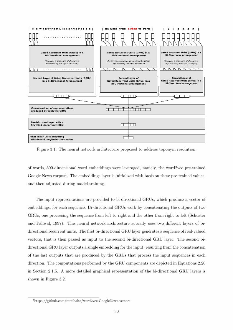
Figure 3.1: The neural network architecture proposed to address toponym resolution.

of words, 300-dimensional word embeddings were leveraged, namely, the word2vec pre-trained

Google News corpus1. The embeddings layer is initialized with basis on these pre-trained values,

and then adjusted during model training.

The input representations are provided to bi-directional GRUs, which produce a vector of

embeddings, for each sequence. Bi-directional GRUs work by concatenating the outputs of two

GRUs, one processing the sequence from left to right and the other from right to left (Schuster

and Paliwal, 1997). This neural network architecture actually uses two different layers of bi-

directional recurrent units. The first bi-directional GRU layer generates a sequence of real-valued

vectors, that is then passed as input to the second bi-directional GRU layer. The second bi-

directional GRU layer outputs a single embedding for the input, resulting from the concatenation

of the last outputs that are produced by the GRUs that process the input sequences in each

direction. The computations performed by the GRU components are depicted in Equations 2.20

in Section 2.1.5. A more detailed graphical representation of the bi-directional GRU layers is

shown in Figure 3.2.

1https://github.com/mmihaltz/word2vec-GoogleNews-vectors

30

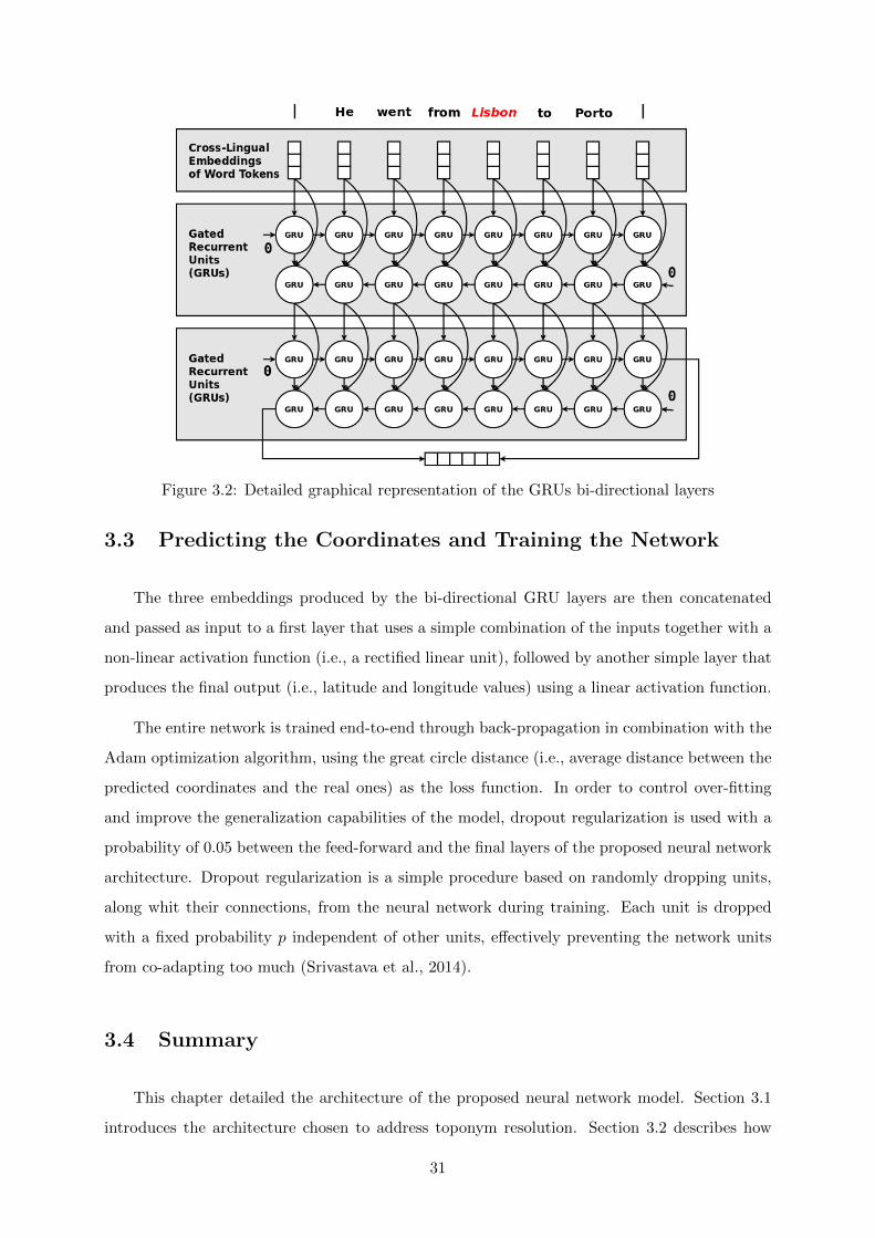
Figure 3.2: Detailed graphical representation of the GRUs bi-directional layers

3.3 Predicting the Coordinates and Training the Network

The three embeddings produced by the bi-directional GRU layers are then concatenated

and passed as input to a first layer that uses a simple combination of the inputs together with a

non-linear activation function (i.e., a rectified linear unit), followed by another simple layer that

produces the final output (i.e., latitude and longitude values) using a linear activation function.

The entire network is trained end-to-end through back-propagation in combination with the

Adam optimization algorithm, using the great circle distance (i.e., average distance between the

predicted coordinates and the real ones) as the loss function. In order to control over-fitting

and improve the generalization capabilities of the model, dropout regularization is used with a

probability of 0.05 between the feed-forward and the final layers of the proposed neural network

architecture. Dropout regularization is a simple procedure based on randomly dropping units,

along whit their connections, from the neural network during training. Each unit is dropped

with a fixed probability p independent of other units, effectively preventing the network units

from co-adapting too much (Srivastava et al., 2014).

3.4 Summary

This chapter detailed the architecture of the proposed neural network model. Section 3.1

introduces the architecture chosen to address toponym resolution. Section 3.2 describes how

31

the input sequences are processed to produce representations. The usage of bi-directional GRUs

ensures that the context of each toponym is captured. Finally, Section 3.3 explains how the

prediction of the geographic coordinates is done and describes the process behind training the

model.

32

4Experimental Evaluation

Deep neural network architectures, such as the one proposed in this dissertation, have

successfully been applied to difficult challenges involving modeling sequences of text, such as

language modeling, machine translation, or even measuring semantic similarity. Through ex-

periments, the goal was to assess if indeed one such model could improve performance over

state-of-the-art toponym resolution techniques. A Python library named Keras1 was used for

implementing the neural network architecture introduced in Chapter 3, and then leveraged some

previous works datasets and also some created for the purpose of this work, to evaluate its per-

formance.

This chapter describes the experimental evaluation of the proposed method. Section 4.1

presents a statistical characterization of the datasets that supported the tests, together with

the considered evaluation metrics. Sections 4.2 and 4.3 present and discuss the obtained results

with the different approaches over the datasets used. Finally, Section 4.4 gives an overview of

the results that were obtained.

4.1 Datasets and Evaluation Metrics

The experiments relied on multiple datasets, each one consisting in annotated sentences

containing toponyms with their respective geographic coordinates. The datasets used in the

experiments were the following:

• TR-CoNLL: The TR-CoNLL corpus (Leidner, 2008) contains 946 REUTERS news ar-

ticles published in August 1996. Since this is a relatively small dataset, three-fold cross-

validation was performed to avoid overfiting. This corpus were provided by the author.

• WOTR: The WarOfTheRebellion (DeLozier et al., 2016) corpus consists in geoannotated

data from the War Of The Rebellion (a large set of American Civil War archives). The

1https://keras.io

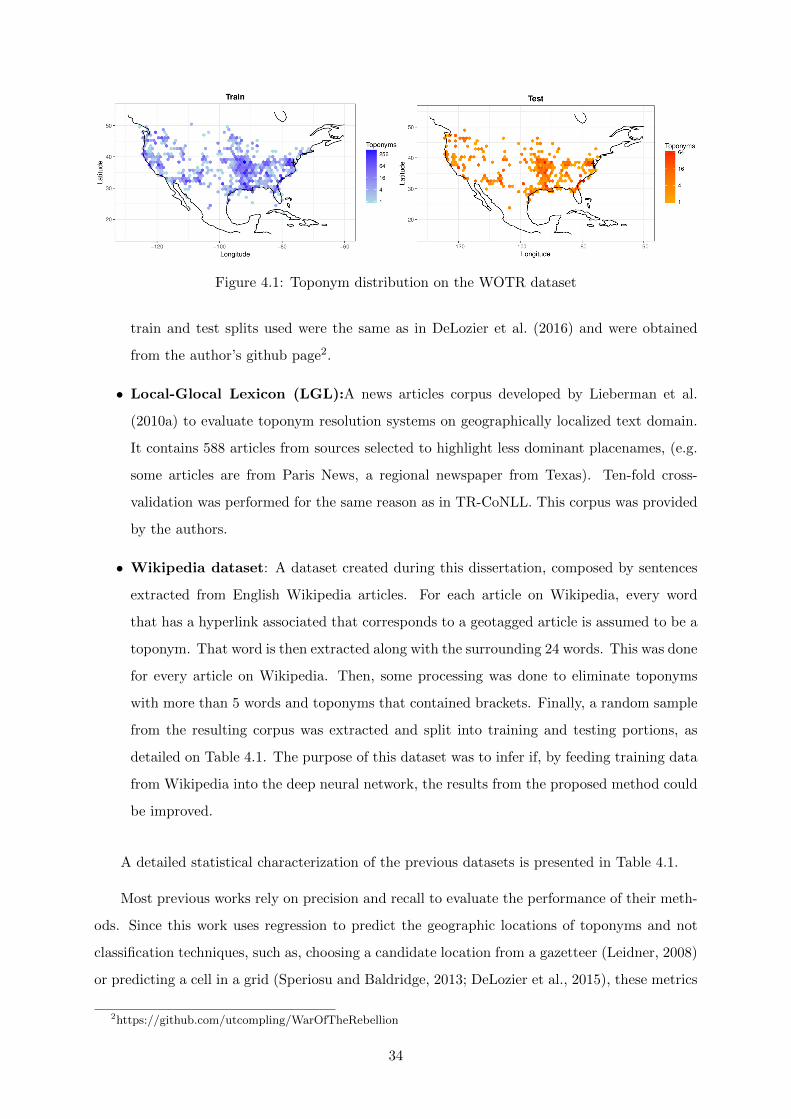
Figure 4.1: Toponym distribution on the WOTR dataset

train and test splits used were the same as in DeLozier et al. (2016) and were obtained

from the author’s github page2.

• Local-Glocal Lexicon (LGL):A news articles corpus developed by Lieberman et al.

(2010a) to evaluate toponym resolution systems on geographically localized text domain.

It contains 588 articles from sources selected to highlight less dominant placenames, (e.g.

some articles are from Paris News, a regional newspaper from Texas). Ten-fold cross-

validation was performed for the same reason as in TR-CoNLL. This corpus was provided

by the authors.

• Wikipedia dataset: A dataset created during this dissertation, composed by sentences

extracted from English Wikipedia articles. For each article on Wikipedia, every word

that has a hyperlink associated that corresponds to a geotagged article is assumed to be a

toponym. That word is then extracted along with the surrounding 24 words. This was done

for every article on Wikipedia. Then, some processing was done to eliminate toponyms

with more than 5 words and toponyms that contained brackets. Finally, a random sample

from the resulting corpus was extracted and split into training and testing portions, as

detailed on Table 4.1. The purpose of this dataset was to infer if, by feeding training data

from Wikipedia into the deep neural network, the results from the proposed method could

be improved.

A detailed statistical characterization of the previous datasets is presented in Table 4.1.

Most previous works rely on precision and recall to evaluate the performance of their meth-

ods. Since this work uses regression to predict the geographic locations of toponyms and not

classification techniques, such as, choosing a candidate location from a gazetteer (Leidner, 2008)

or predicting a cell in a grid (Speriosu and Baldridge, 2013; DeLozier et al., 2015), these metrics

2https://github.com/utcompling/WarOfTheRebellion

34

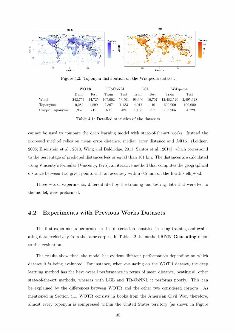
Figure 4.2: Toponym distribution on the Wikipedia dataset.

WOTR TR-CoNLL LGL Wikipedia

Train Test Train Test Train Test Train Test

Words 242,754 44,725 107,002 53,501 96,366 10,707 12,482,520 2,495,628

Toponyms 10,280 1,899 2,867 1,433 4,017 446 600,000 100,000

Unique Toponyms 1,952 712 608 424 1,138 297 108,965 34,729

Table 4.1: Detailed statistics of the datasets

cannot be used to compare the deep learning model with state-of-the-art works. Instead the

proposed method relies on mean error distance, median error distance and A@161 (Leidner,

2008; Eisenstein et al., 2010; Wing and Baldridge, 2011; Santos et al., 2014), which correspond

to the percentage of predicted distances less or equal than 161 km. The distances are calculated

using Vincenty’s formulae (Vincenty, 1975), an iterative method that computes the geographical

distance between two given points with an accuracy within 0.5 mm on the Earth’s ellipsoid.

Three sets of experiments, differentiated by the training and testing data that were fed to

the model, were preformed.

4.2 Experiments with Previous Works Datasets

The first experiments performed in this dissertation consisted in using training and evalu-

ating data exclusively from the same corpus. In Table 4.2 the method RNN-Geocoding refers

to this evaluation.

The results show that, the model has evident different performances depending on which

dataset it is being evaluated. For instance, when evaluating on the WOTR dataset, the deep

learning method has the best overall performance in terms of mean distance, beating all other

state-of-the-art methods, whereas with LGL and TR-CoNNL it performs poorly. This can

be explained by the differences between WOTR and the other two considered corpora. As

mentioned in Section 4.1, WOTR consists in books from the American Civil War, therefore,

almost every toponym is compressed within the United States territory (as shown in Figure

35

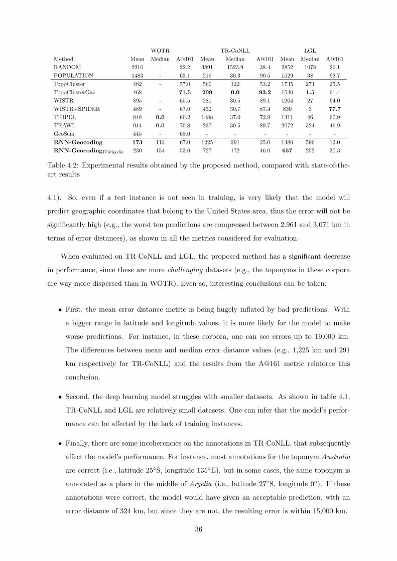
WOTR TR-CoNLL LGL

Method Mean Median A@161 Mean Median A@161 Mean Median A@161

RANDOM 2216 - 22.2 3891 1523.9 38.4 2852 1078 26.1

POPULATION 1483 - 63.1 219 30.3 90.5 1529 38 62.7

TopoCluster 482 - 57.0 560 122 53.2 1735 274 25.5

TopoClusterGaz 468 - 71.5 209 0.0 93.2 1540 1.5 61.4

WISTR 895 - 65.5 281 30.5 89.1 1264 27 64.0

WISTR+SPIDER 489 - 67.0 432 30.7 87.4 830 3 77.7

TRIPDL 848 0.0 60.2 1488 37.0 72.9 1311 46 60.9

TRAWL 944 0.0 70.8 237 30.5 89.7 2072 324 46.9

GeoSem 445 - 68.0 - - - - - -

RNN-Geocoding 173 113 67.0 1225 291 25.0 1480 596 12.0

RNN-GeocodingWikipedia 230 154 53.0 727 172 46.0 657 252 30.3

Table 4.2: Experimental results obtained by the proposed method, compared with state-of-the-art results

4.1). So, even if a test instance is not seen in training, is very likely that the model will

predict geographic coordinates that belong to the United States area, thus the error will not be

significantly high (e.g., the worst ten predictions are compressed between 2.961 and 3,071 km in

terms of error distances), as shown in all the metrics considered for evaluation.

When evaluated on TR-CoNLL and LGL, the proposed method has a significant decrease

in performance, since these are more challenging datasets (e.g., the toponyms in these corpora

are way more dispersed than in WOTR). Even so, interesting conclusions can be taken:

• First, the mean error distance metric is being hugely inflated by bad predictions. With

a bigger range in latitude and longitude values, it is more likely for the model to make

worse predictions. For instance, in these corpora, one can see errors up to 19,000 km.

The differences between mean and median error distance values (e.g., 1,225 km and 291

km respectively for TR-CoNLL) and the results from the A@161 metric reinforce this

conclusion.

• Second, the deep learning model struggles with smaller datasets. As shown in table 4.1,

TR-CoNLL and LGL are relatively small datasets. One can infer that the model’s perfor-

mance can be affected by the lack of training instances.

• Finally, there are some incoherencies on the annotations in TR-CoNLL, that subsequently

affect the model’s performance. For instance, most annotations for the toponym Australia

are correct (i.e., latitude 25◦S, longitude 135◦E), but in some cases, the same toponym is

annotated as a place in the middle of Argelia (i.e., latitude 27◦S, longitude 0◦). If these

annotations were correct, the model would have given an acceptable prediction, with an

error distance of 324 km, but since they are not, the resulting error is within 15,000 km.

36

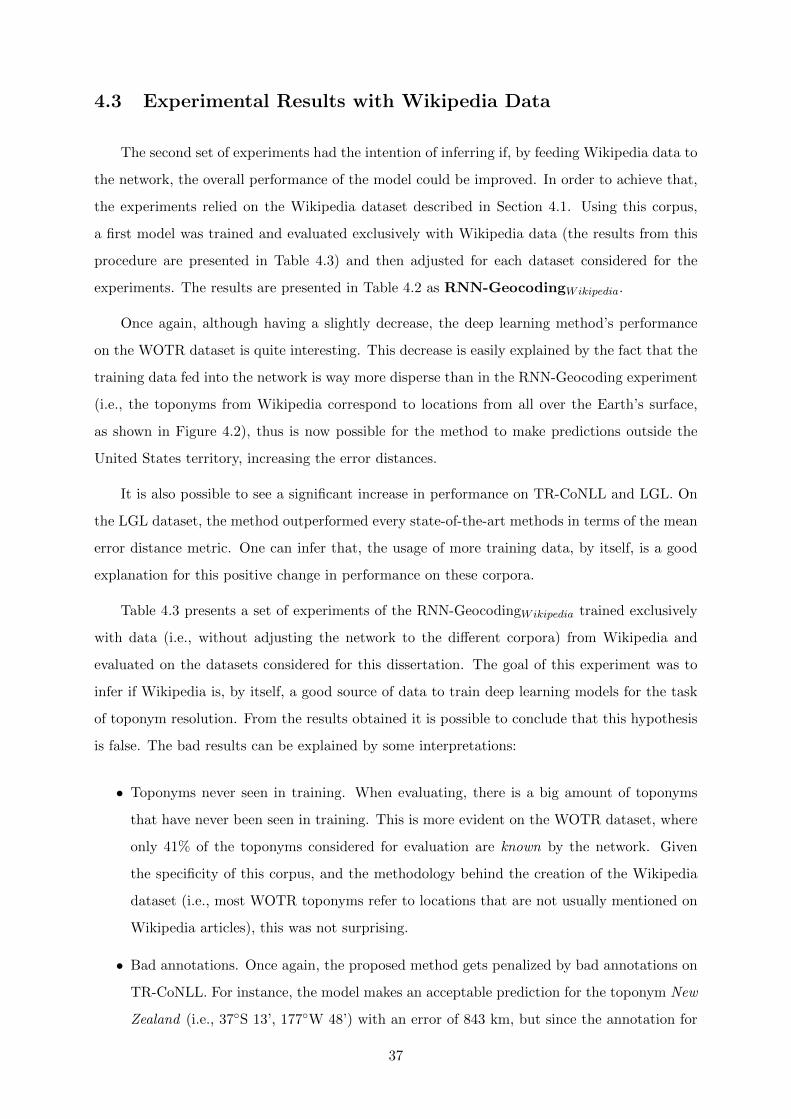
4.3 Experimental Results with Wikipedia Data

The second set of experiments had the intention of inferring if, by feeding Wikipedia data to

the network, the overall performance of the model could be improved. In order to achieve that,

the experiments relied on the Wikipedia dataset described in Section 4.1. Using this corpus,

a first model was trained and evaluated exclusively with Wikipedia data (the results from this

procedure are presented in Table 4.3) and then adjusted for each dataset considered for the

experiments. The results are presented in Table 4.2 as RNN-GeocodingWikipedia.

Once again, although having a slightly decrease, the deep learning method’s performance

on the WOTR dataset is quite interesting. This decrease is easily explained by the fact that the

training data fed into the network is way more disperse than in the RNN-Geocoding experiment

(i.e., the toponyms from Wikipedia correspond to locations from all over the Earth’s surface,

as shown in Figure 4.2), thus is now possible for the method to make predictions outside the

United States territory, increasing the error distances.

It is also possible to see a significant increase in performance on TR-CoNLL and LGL. On

the LGL dataset, the method outperformed every state-of-the-art methods in terms of the mean

error distance metric. One can infer that, the usage of more training data, by itself, is a good

explanation for this positive change in performance on these corpora.

Table 4.3 presents a set of experiments of the RNN-GeocodingWikipedia trained exclusively

with data (i.e., without adjusting the network to the different corpora) from Wikipedia and

evaluated on the datasets considered for this dissertation. The goal of this experiment was to

infer if Wikipedia is, by itself, a good source of data to train deep learning models for the task

of toponym resolution. From the results obtained it is possible to conclude that this hypothesis

is false. The bad results can be explained by some interpretations:

• Toponyms never seen in training. When evaluating, there is a big amount of toponyms

that have never been seen in training. This is more evident on the WOTR dataset, where

only 41% of the toponyms considered for evaluation are known by the network. Given

the specificity of this corpus, and the methodology behind the creation of the Wikipedia

dataset (i.e., most WOTR toponyms refer to locations that are not usually mentioned on

Wikipedia articles), this was not surprising.

• Bad annotations. Once again, the proposed method gets penalized by bad annotations on

TR-CoNLL. For instance, the model makes an acceptable prediction for the toponym New

Zealand (i.e., 37◦S 13’, 177◦W 48’) with an error of 843 km, but since the annotation for

37

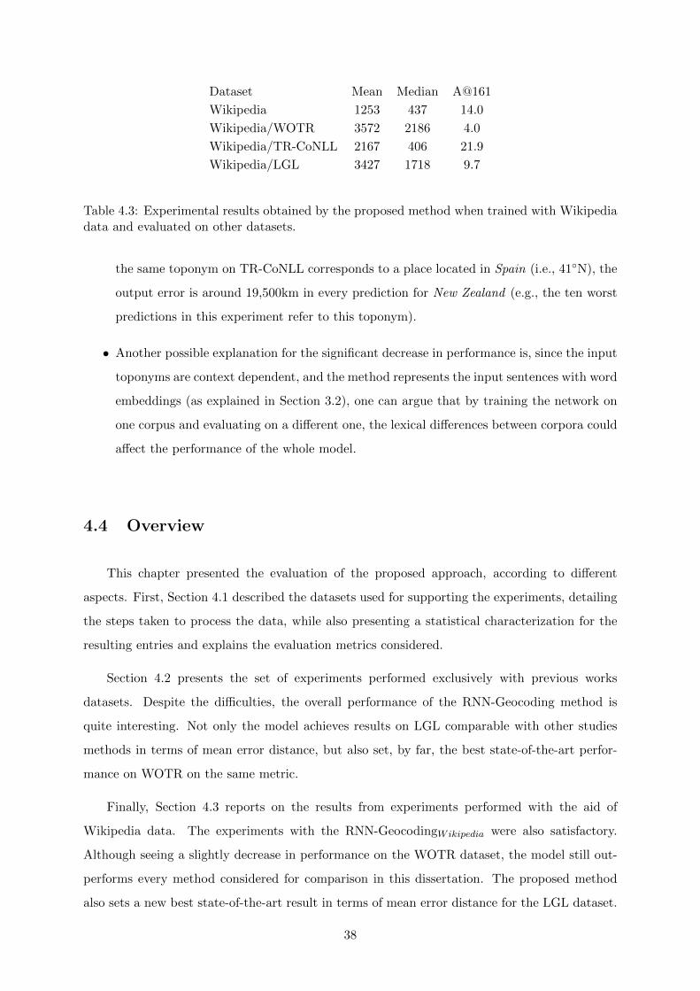
Dataset Mean Median A@161

Wikipedia 1253 437 14.0

Wikipedia/WOTR 3572 2186 4.0

Wikipedia/TR-CoNLL 2167 406 21.9

Wikipedia/LGL 3427 1718 9.7

Table 4.3: Experimental results obtained by the proposed method when trained with Wikipediadata and evaluated on other datasets.

the same toponym on TR-CoNLL corresponds to a place located in Spain (i.e., 41◦N), the

output error is around 19,500km in every prediction for New Zealand (e.g., the ten worst

predictions in this experiment refer to this toponym).

• Another possible explanation for the significant decrease in performance is, since the input

toponyms are context dependent, and the method represents the input sentences with word

embeddings (as explained in Section 3.2), one can argue that by training the network on

one corpus and evaluating on a different one, the lexical differences between corpora could

affect the performance of the whole model.

4.4 Overview

This chapter presented the evaluation of the proposed approach, according to different

aspects. First, Section 4.1 described the datasets used for supporting the experiments, detailing

the steps taken to process the data, while also presenting a statistical characterization for the

resulting entries and explains the evaluation metrics considered.

Section 4.2 presents the set of experiments performed exclusively with previous works

datasets. Despite the difficulties, the overall performance of the RNN-Geocoding method is

quite interesting. Not only the model achieves results on LGL comparable with other studies

methods in terms of mean error distance, but also set, by far, the best state-of-the-art perfor-

mance on WOTR on the same metric.

Finally, Section 4.3 reports on the results from experiments performed with the aid of

Wikipedia data. The experiments with the RNN-GeocodingWikipedia were also satisfactory.

Although seeing a slightly decrease in performance on the WOTR dataset, the model still out-

performs every method considered for comparison in this dissertation. The proposed method

also sets a new best state-of-the-art result in terms of mean error distance for the LGL dataset.

38

The results from this method also prove that feeding Wikipedia data into deep learning models,

can have significant impact on NLP tasks such as toponym resolution.

39

40

5ConclusionsThis dissertation presented a deep learning method for predicting geographic coordinates of

placenames (i.e. toponyms) given their context (i.e. surrounding words). This chapter overviews

the main contributions, and highlights possible directions for future work.

5.1 Overview on the Contributions

Results show that although toponym resolution is a difficult task, due to the large number

of placenames and their ambiguity, the method obtained interesting performances in terms of

mean and median error distances. Given the results, it is possible to argue that this approach

can indeed, in some cases, contribute to better predictions of geographic coordinates.

The main contributions of this dissertation are as follow:

• English Wikipedia dataset: This new dataset was collected from the data dump from

Wikimedia Foundation. It is composed by 600,000 geotagged sentences extracted from

Wikipedia articles (as detailed in Section 4.1). This dataset is oriented for NLP studies,

focused on geotagging tasks, since every sentence is labeled with the corresponding geo-

graphic coordinates. With free distribution, other authors can use this corpus to aid their

methods and try to improve the obtained results in this work.

• A new method for toponym resolution: The proposed methodology introduces a new

model in the automatic toponym resolution task. As stated before, this model achieved

interesting results when compared with state-of-the-art performances. Despite this results,

it is possible that with some future adjustments (e.g. as stated in Section 5.2), the proposed

model performance can be improved.

• Experiments with different datasets: The experiments performed on WOTR, TR-

CoNLL and LGL datasets, prove that the proposed model can achieve and surpass state-

of-the-art results. Specifically, on WOTR and LGL datasets, new best performances in

terms of mean error distance were set as a result of this dissertation.

5.2 Future Work

Despite the interesting results there are also many ideas for future work, since different

options can be considered for improving the neural network architecture. The proposed neural

architecture leverages GRUs to encode sequences of words, but other types of recurrent nodes

have also recently been proposed. For instance, the Minimal Gated Unit approach Zhou et al.

(2016); Heck and Salem (2017) relies on a simplified model with just a single gate. Having less

parameters to train can contribute to improving the model effectiveness. In contrast, Multi-

Function Recurrent Units (Mu-FuRUs) adopt an elaborate gating mechanism that allows for

additional differentiable functions as composition operations, leading to models that can better

capture the nuances involved in encoding word sequences (Weissenborn and Rocktaschel, 2016).

Other alternatives include Long Short-Term Memory (LSTM) networks with coupled gates (Greff

et al., 2016), Structurally Constrained Recurrent Networks (Mikolov et al., 2014), IRNNs (Le

et al., 2015), and many other LSTM or GRU variants (Greff et al., 2016; Jozefowicz et al., 2015).

Recent studies had relevant results with the usage of attention mechanisms on deep neural

networks for document classification (Shimaoka et al., 2016; Yang et al., 2016). The attention

mechanism provides a way of giving more or less importance to each word, allowing a model to

focus on those that matter th most to the classification of each instance. It would be interesting to

apply this technique on the proposed method, in addition to approaching the toponym resolution

problem as a classification task (e.g., by predicting a cell on the Earth’s surface) similarly to

Speriosu and Baldridge (2013) and DeLozier et al. (2015).

Another addition to the deep learning model proposed in this dissertation would be following

the inspiration of Rahimi et al. (2017), by using mixed density networks (MDNs: Bishop (1994))

to generate a mixture model in the form of a probability distribution over all toponyms.

Due to limited resources, the Wikipedia dataset had to be randomly sampled to the size

presented in Table 4.1. However, it is possible to create bigger datasets from the Wikipedia data

dump (e.g., the initial dataset had more than 16 million sentences). It would be interesting to

use a bigger dataset and infer if the overall model’s performance is improved. Also, Wikipedia

dumps from other languages could be used to train the model to have the ability for resolving

toponyms in different dialects. In order to perform such training, multilingual embeddings could

be leveraged, such as the ones provided by Ferreira et al. (2016).

42

Bibliography

Al-Rfou, R., Kulkarni, V., Perozzi, B., and Skiena, S. (2015). Polyglot-ner: Massive multilingual

named entity recognition. In Proceedings of the Society for Industrial and Applied Mathematics

Conference on Data Mining.

Amitay, E., Har’El, N., Sivan, R., and Soffer, A. (2004). Web-a-Where: Geotagging Web

Content. In Proceedings of the Association for Computing Machinery SIGIR Conference on

Research and Development in Information Retrieval.

Ardanuy, M. C. and Sporleder, C. (2017). Toponym Disambiguation in Historical Documents

Using Semantic and Geographic Features. In Proceedings of the International Conference on

Digital Access to Textual Cultural Heritage.

Bishop, C. M. (1994). Mixture density networks.

Bowman, S. R., Angeli, G., Potts, C., and Manning, C. D. (2015). A Large Annotated Corpus

for Learning Natural Language Inference. arXiv preprint arXiv:1508.05326.

Breiman, L. (2001). Random Forests. Machine learning, 45(1).

Broder, A. Z. (1997). On the Resemblance and Containment of Documents. In Proceedings of

the Compression and Complexity of Sequences.

Burges, C. J. C. (2010). From Ranknet to Lambdarank to Lambdamart: An Overview. Learning,

11.

Chung, J., Gulcehre, C., Cho, K., and Bengio, Y. (2014). Empirical Evaluation of Gated

Recurrent Neural Networks on Sequence Modeling. arXiv preprint arXiv:1412.3555.

DeLozier, G., Baldridge, J., and London, L. (2015). Gazetteer-Independent Toponym Resolution

Using Geographic Word Profiles. In Proceedings of the Conference of the Association for the

Advancement of Artificial Intelligence.

DeLozier, G., Wing, B., Baldridge, J., and Nesbit, S. (2016). Creating a Novel Geolocation

Corpus from Historical Texts. In Proceedings of the Linguistic Annotation Workshop of the

Association for Computational Linguistics.

43

Eisenstein, J., O’Connor, B., Smith, N. A., and Xing, E. P. (2010). A Latent Variable Model

for Geographic Lexical Variation. In Proceedings of the Conference on Empirical Methods in

Natural Language Processing. Association for Computational Linguistics.

Ferreira, D. C., Martins, A. F. T., and Almeida, M. S. C. (2016). Jointly Learning to Embed

and Predict with Multiple Languages. Association for Computational Linguistics, 1.

Finkel, J. R., Grenager, T., and Manning, C. (2005). Incorporating Non-local Information into

Information Extraction Systems by Gibbs Sampling. In Proceedings of the Annual Meeting of

the Association for Computational Linguistics.

Gale, W. A., Church, K. W., and Yarowsky, D. (1992). One Sense Per Discourse. In Proceedings

of the Workshop on Speech and Natural Language.

Goodfellow, I., Bengio, Y., and Courville, A. (2016). Deep Learning. MIT Press.

Greff, K., Srivastava, R. K., Koutnık, J., Steunebrink, B. R., and Schmidhuber, J. (2016). LSTM:

A Search Space Odyssey. IEEE Transactions on Neural Networks and Learning Systems,

PP(99).

Gregory, I., Donaldson, C., Murrieta-Flores, P., and Rayson, P. (2015). Geoparsing, GIS, and

Textual Analysis: Current Developments in Spatial Humanities Research. International Jour-

nal of Humanities and Arts Computing, 9(1).

Grover, C., Tobin, R., Byrne, K., Woollard, M., Reid, J., Dunn, S., and Ball, J. (2010). Use

of the Edinburgh Geoparser for Georeferencing Digitized Historical Collections. Philosophical

Transactions. Series A, Mathematical, Physical, and Engineering Sciences, 368(1925).

Han, X., Sun, L., and Zhao, J. (2011). Collective Entity Linking in Web Text: A Graph-based

Method. In Proceedings of the International Association for Computing Machinery SIGIR

Conference on Research and Development in Information Retrieval.

Heck, J. and Salem, F. M. (2017). Simplified Minimal Gated Unit Variations for Recurrent

Neural Networks. arXiv preprint arXiv:1701.03452.

Hermann, K. M. and Blunsom, P. (2013). Multilingual Distributed Representations Without

Word Alignment. arXiv preprint arXiv:1312.6173.

Hochreiter, S. and Schmidhuber, J. (1997). Long Short-Term Memory. Neural Computing, 9(8).

44

Ji, H. and Grishman, R. (2011). Knowledge Base Population: Successful Approaches and Chal-

lenges. In Proceedings of the Annual Meeting of the Association for Computational Linguistics:

Human Language Technologies.

Jozefowicz, R., Zaremba, W., and Sutskever, I. (2015). An Empirical Exploration of Recurrent

Network Architectures. In Proceedings of the International Conference on Machine Learning.

Juan, A. and Ney, H. (2002). Reversing and Smoothing the Multinomial Naive Bayes Text

Classifer. In Proceedings of the International Workshop on Pattern Recognition in Information

Systems.

Kelley, H. J. (1960). Gradient Theory of Optimal Flight Paths. Ars Journal, 30(10).

Kingma, D. and Ba, J. (2015). Adam: A Method for Stochastic Optimization. In Proceedings

of the International Conference for Learning Representations.

Kullback, S. and Leibler, R. A. (1951). On Information and Sufficiency. The annals of mathe-

matical statistics, 22(1).

Le, Q. V., Jaitly, N., and Hinton, G. E. (2015). A Simple Way to Initialize Recurrent Networks

of Rectified Linear Units. arXiv preprint arXiv:1504.00941.

LeCun, Y., Bengio, Y., and Hinton, G. (2015). Deep learning. Nature, 521(7553).

Leidner, J. L. (2007). Toponym Resolution in Text: Annotation, Evaluation and Applications

of Spatial Grounding. In Proceedings of Association for Computing Machinery.

Leidner, J. L. (2008). Toponym Resolution in Text: Annotation, Evaluation and Applications

of Spatial Grounding of Place Names. School of Informatics University of Edinburgh.

Lidstone, G. (1920). Note on the General Case of the Bayes–Laplace Formula for Inductive or

a Posteriori Probabilities. Transactions of the Faculty of Actuaries, 8.

Lieberman, M. D. and Samet, H. (2011). Multifaceted Toponym Recognition for Streaming

News. In Proceedings of the International Association for Computing Machinery SIGIR Con-

ference on Research and Development in Information Retrieval.

Lieberman, M. D. and Samet, H. (2012). Adaptive Context Features for Toponym Resolution in

Streaming News. In Proceedings of the International Association for Computing Machinery

SIGIR Conference on Research and Development in Information Retrieval.

45

Lieberman, M. D., Samet, H., and Sankaranarayanan, J. (2010a). Geotagging with Local Lexi-

cons to Build Indexes for Textually-specified Spatial Data. In Proceedings of the International

Conference on Data Engineering.

Lieberman, M. D., Samet, H., Sankaranarayanan, J., and Sperling, J. (2009). Spatio-textual

Spreadsheets: Geotagging via Spatial Coherence. In Proceedings of the annual Association

for Computing Machinery SIGSPATIAL International Conference on Advances in Geographic

Information Systems.

Lieberman, M. D., Samet, H., and Sankaranayananan, J. (2010b). Geotagging: Using Proximity,

Sibling, and Prominence Clues to Understand Comma Groups. In Proceedings of the Workshop

on Geographic Information Retrieval.

Lippmann, R. (1987). An Introduction to Computing with Neural Nets. IEEE ASSP magazine,

4(2).

Liu, Y., Sun, C., Lin, L., and Wang, X. (2016). Learning Natural Language Inference using

Bidirectional LSTM Model and Inner-Attention. arXiv preprint arXiv:1605.09090.

Mani, I., Hitzeman, J., Richer, J., Harris, D., Quimby, R., and Wellner, B. (2008). SpatialML:

Annotation Scheme, Corpora, and Tools. In Proceedings of the International Conference on

Language Resources and Evaluation.

Mikolov, T., Joulin, A., Chopra, S., Mathieu, M., and Ranzato, M. (2014). Learning Longer

Memory in Recurrent Neural Networks. arXiv preprint arXiv:1412.7753.

Mikolov, T., Sutskever, I., Chen, K., Corrado, G. S., and Dean, J. (2013). Distributed Represen-

tations of Words and Phrases and their Compositionality. In Proceedings of the International

Conference on Neural Information Processing Systems.

Morin, F. and Bengio, Y. (2005). Hierarchical Probabilistic Neural Network Language Model.

In Proceedings of the Artificial Intelligence and Statistics Conference.

Mueller, J. and Thyagarajan, A. (2016). Siamese Recurrent Architectures for Learning Sentence

Similarity. In Proceedings of the Association for the Advancement of Artificial Intelligence.

Ord, J. K. and Getis, A. (1995). Local Spatial Autocorrelation Statistics: Distributional Issues

and an Application. Geographical analysis, 27(4).

P. Murphy, K. (2012). Machine Learning: A Probabilistic Perspective.

46

Rahimi, A., Baldwin, T., and Cohn, T. (2017). Continuous Representation of Location for

Geolocation and Lexical Dialectology using Mixture Density Networks. arxiv preprint arXiv:

arXiv:1708.04358.

Rauch, E., Bukatin, M., and Baker, K. (2003). A Confidence-based Framework for Disambigua-

tion Geographic Terms. In Proceedings of the Conference of the North American Chapter of

the Association for Computational Linguistics on Human Language Technology.

Rocktaschel, T., Grefenstette, E., Hermann, K. M., Kocisky, T., and Blunsom, P. (2016). Rea-

soning About Entailment with Neural Attention. In Proceedings of the International Confer-

ence on Learning Representations.

Rosenblatt, F. (1958). The Perceptron: a Probabilistic Model for Information Storage and

Organization in the Brain. Psychological Review, 65(6).

Rumelhart, D. E., Hinton, G. E., and Williams, R. J. (1988). Learning Representations by

Back-propagating Errors. Cognitive modeling, 5(3).

Salton, G., Wong, A., and Yang, C. S. (1975). A Vector Space Model for Automatic Indexing.

Communications of the Association for Computing Machinery, 18(11).

Sankaranarayanan, J., Samet, H., Teitler, B. E., Lieberman, M. D., and Sperling, J. (2009).

TwitterStand: News in Tweets. In Proceedings of the Association for Computing Machinery

SIGSPATIAL International Conference on Advances in Geographic Information Systems.

Santos, J., Anastacio, I., and Martins, B. (2014). Using Machine Learning Methods for Disam-

biguating Place References in Textual Documents. GeoJournal, 80(3).

Santos, R., Murrieta-Flores, P., and Martins, B. (2017). Learning to Combine Multiple String

Similarity Metrics for Effective Toponym Matching. (currently under review).

Schmidhuber, J. (2015). Deep Learning in Neural Networks: An Overview. Neural Networks,

61(1).

Schuster, M. and Paliwal, K. K. (1997). Bidirectional Recurrent Neural Networks. IEEE Trans-

actions on Signal Processing, 45(11).

Sebastiani, F. (2002). Machine Learning in Automated Text Categorization. Association for

Computing Machinery Computing Surveys, 34(1).

Shen, W., Wang, J., and Han, J. (2015). Entity Linking with a Knowledge Base: Issues,

Techniques, and Solutions. IEEE Transactions on Knowledge and Data Engineering, 27(2).

47

Shimaoka, S., Stenetorp, P., Inui, K., and Riedel, S. (2016). Neural Architectures for Fine-

grained Entity Type Classification. arXiv preprint arXiv:1606.01341.

Speriosu, M. and Baldridge, J. (2013). Text-Driven Toponym Resolution using Indirect Supervi-

sion. In Proceedings of the Annual Meeting of the Association for Computational Linguistics.

Srivastava, N., Hinton, G., Krizhevsky, A., Sutskever, I., and Salakhutdinov, R. (2014). Dropout:

A Simple Way to Prevent Neural Networks from Overfitting. Journal of Machine Learning

Research, 15(1).

Teitler, B. E., Lieberman, M. D., Panozzo, D., Sankaranarayanan, J., Samet, H., and Sperling,

J. (2008). NewsStand: A New View on News. In Proceedings of the Association for Computing

Machinery SIGSPATIAL International Conference on Advances in Geographic Information

Systems.

Turian, J., Ratinov, L., and Bengio, Y. (2010). Word Representations: a Simple and General

Method for Semi-supervised Learning. In Proceedings of the annual meeting of the Association

for Computational Linguistics.

Vincenty, T. (1975). Direct and Inverse Solutions of Geodesics on the Ellipsoid with Application

of Nested Equations. Survey Review, 22(176).

Volz, R., Kleb, J., and Mueller, W. (2007). Towards Ontology-based Disambiguation of Geo-

graphical Identifiers. In Proceedings of CEUR Workshop.

Wan, S., Lan, Y., Guo, J., Xu, J., Pang, L., and Cheng, X. (2016). A Deep Architecture for

Semantic Matching with Multiple Positional Sentence Representations. In Proceedings of the

Association for the Advancement of Artificial Intelligence.

Weissenborn, D. and Rocktaschel, T. (2016). MuFuRU: The Multi-Function Recurrent Unit.

In Proceedings of the Association for Computational Linguistics Workshop on Representation

Learning for NLP.

Wing, B. P. and Baldridge, J. (2011). Simple Supervised Document Geolocation with Geodesic

Grids. In Proceedings of the Annual Meeting of the Association for Computational Linguistics.

Yang, Z., Yang, D., Dyer, C., He, X., Smola, A. J., and Hovy, E. H. (2016). Hierarchical

Attention Networks for Document Classification. In Proceedings of the Conference of the

North American Chapter of the Association for Computational Linguistic.

48

Yin, W. and Schutze, H. (2015). Convolutional Neural Network for Paraphrase Identification.

In Proceedings of the Conference of the North American Chapter of the Association for Com-

putational Linguistics.

Zhou, G.-B., Wu, J., Zhang, C.-L., and Zhou, Z.-H. (2016). Minimal Gated Unit for Recurrent

Neural Networks. International Journal of Automation and Computing, 13(3).

Zou, W. Y., Socher, R., Cer, D. M., and Manning, C. D. (2013). Bilingual Word Embeddings for

Phrase-Based Machine Translation. In Proceedings of Empirical Methods on Natural Language

Processing.

49