Topology Optimization of Energy Harvesting Devices – The ...
26
D. Hoffmann / 28.05.10 / Slide 1 www.hsg-imit.de Topology Optimization of Energy Harvesting Devices – The Quest for Maximum Power Output Daniel Hoffmann Institut für Mikro- und Informationstechnik der Hahn-Schickard Gesellschaft e.V. HSG-IMIT Wilhelm-Schickard-Str. 10, D-78052 Villingen-Schwenningen, Germany phone: +49 7721 943-187 fax: +49 7721 943-210 email: [email protected]
Transcript of Topology Optimization of Energy Harvesting Devices – The ...

D. Hoffmann / 28.05.10 / Slide 1www.hsg-imit.de
Topology Optimization of Energy Harvesting Devices –
The Quest for Maximum Power Output
Daniel HoffmannInstitut für Mikro- und Informationstechnik der Hahn-Schickard Gesellschaft e.V.
HSG-IMITWilhelm-Schickard-Str. 10, D-78052 Villingen-Schwenningen, Germany
phone: +49 7721 943-187 fax: +49 7721 943-210 email: [email protected]

D. Hoffmann / 28.05.10 / Slide 2www.hsg-imit.de
Outline
Introduction to energy harvesting• Motivation• Examples of demonstrators• Energy harvesting from vibrations• Energy conversion principles• Workflow
Optimization of electrostatic energy harvesting devices• Active principle• Design constraints• Optimization using modeFRONTIER• Conclusions
D. Hoffmann / 28.05.10 / Slide 3www.hsg-imit.de
Motivation
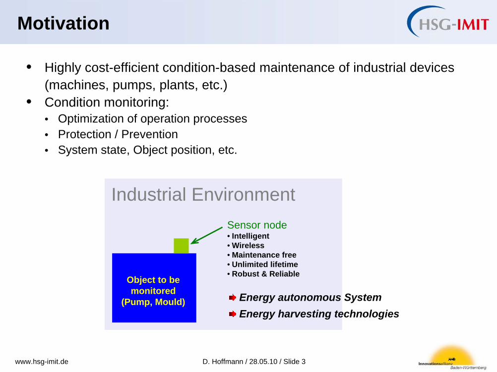
Industrial Environment
Object to be monitored
(Pump, Mould)
Sensor node• Intelligent• Wireless• Maintenance free• Unlimited lifetime• Robust & Reliable
• Highly cost-efficient condition-based maintenance of industrial devices (machines, pumps, plants, etc.)
• Condition monitoring:• Optimization of operation processes• Protection / Prevention• System state, Object position, etc.
Energy autonomous SystemEnergy harvesting technologies

D. Hoffmann / 28.05.10 / Slide 4www.hsg-imit.de
Motivation
• Energy Harvesting Harvesting of electrical energy through conversion of ambient non-electrical energy
Radiation (light), thermal gradients, kinetic motions (vibrations)
• Research and Development at HSG-IMITDevelopment of application specific vibration generators
Continuous improvement of performance (effectiveness & efficiency)
Broadband systems, adaptive systems

D. Hoffmann / 28.05.10 / Slide 5www.hsg-imit.de
Intelligent Fluid Quick Connector
Vibration transducer

D. Hoffmann / 28.05.10 / Slide 6www.hsg-imit.de
Concrete Products Mould

D. Hoffmann / 28.05.10 / Slide 7www.hsg-imit.de
Energy Harvesting in Railroad Applications

D. Hoffmann / 28.05.10 / Slide 8www.hsg-imit.de
• Coupling of kinetic vibration energy• Mechanical to electrical energy conversion• High effectiveness of energy conversion• High efficiency of power management circuits• Minimum output ratings: voltage, current, power (given by application)• Size limited to available construction volume (given by application)• Adjustable to the specific conditions of the target environment• Self adaptation to changes in the vibration profile (frequency)• Dynamic long-term stability (reliability, durability)• No affection by environmental influences (temperature, materials,
moisture, )• …
General requirements
Energy Harvesting from Vibrations

D. Hoffmann / 28.05.10 / Slide 9www.hsg-imit.de
Vibration Source
Vibration Generator Electronics Energy
Storage Consumer
Losses LossesLosses
Optimization Efficiency
Optimization Effectiviness
Energy Harvesting from Vibrations
m
me ccc +=k
)(tx
)(tz
)(ty
Generator components• Oscillating mass• Suspension springs• Transduction mechanism

D. Hoffmann / 28.05.10 / Slide 10www.hsg-imit.de
Parameter Electromagnetic Piezoelectric Electrostatic
Voltage (AC Peak) 1 V … 10 V 5 V … 50 V 0.5 V … 5 V Current (AC Peak) 1 mA … 15 mA 10 µA … 200 µA 0.5 µA … 10 µA Power (AC Peak) 1 mW … 150 mW 50 µW … 10 mW 0.2 µW … 50 µW Operation frequency 30 Hz … 500 Hz 50 Hz … 500 Hz 1000 Hz … 5000 Hz Size 3 cm³ … 250 cm³ 5 cm³ … 50 cm³ 0.2 cm³ … 0.5 cm³ Mass of proof mass 10 g … 500 g 1 g … 10 g 500 µg … 1000 µg Displacement limit 0.5 mm … 3 mm 0.5 mm … 1 mm 10 µm … 40 µm
Energy Conversion Principles
+ + + + ++ + + + +
+ ++ +
--
--
--
--
--
--
--m
me ccc +=k
)(tx
)(tz
)(ty
Performance strongly dependent on excitation conditions!

D. Hoffmann / 28.05.10 / Slide 11www.hsg-imit.de
0.2cm³, 1-10µW
200cm³, 100-800mWParameter Electromagnetic Piezoelectric Electrostatic
Excitation 39 m/s² 13 m/s² 59 m/s² Voltage (AC) 9 V 39 V 1.1 V Current (AC) 90 mA 385 µA 1.9 µA Power (AC) 800 mW 15 mW 2.2 µW Frequency 30 Hz 150 Hz 1220 Hz Size 190 cm³ 18 cm³ 0.2 cm³
Energy harvesting from vibrations
Device Range & Examples

D. Hoffmann / 28.05.10 / Slide 12www.hsg-imit.de
Analysis of the target environment
Choice of a transduction mechanism
Modelling, Design and Optimization
Workflow
Manufacturing and Characterization
86 87 88 89 90 91 92 93 94
-200
0
200
Time (s)
acc
(m/s
²)
Acceleration Profile
0 10 20 30 40 50 60 70 80 90 1000
20
40
60
80
Frequency (Hz)
PSD
(dB
/Hz)
Power Spectral Density
86 87 88 89 90 91 92 93 94
-200
0
200
Time (s)
acc
(m/s
²)
Acceleration Profile
0 10 20 30 40 50 60 70 80 90 1000
20
40
60
80
Frequency (Hz)
PSD
(dB
/Hz)
Power Spectral Density
0
0.2
0.4
0.6
0.8
1
1.2
1.4
1.6
1.8
2
40 45 50 55 60 65
Frequency (Hz)
Pow
er (m
W)
Excitation: 2 m/s²
Excitation: 3 m/s²
Excitation: 4 m/s²
N
S I II III IV V VI VII VIII0
2
4
6
8
P opt (m
W)
0 20 40 60 80 100 120 140 160 180 200-60
-40
-20
0
20
40
60
Time (s)
acc
(m/s
²)
Acceleration Profile
0 50 100 150 200 2500
10
20
30
Frequency (Hz)
PSD
(dB
/Hz)
Power Spectral Density
0 20 40 60 80 100 120 140 160 180 200-60
-40
-20
0
20
40
60
Time (s)
acc
(m/s
²)
Acceleration Profile
0 50 100 150 200 2500
10
20
30
Frequency (Hz)
PSD
(dB
/Hz)
Power Spectral Density

D. Hoffmann / 28.05.10 / Slide 13www.hsg-imit.de
• Size: 0.2 cm³• Voltage: (1 – 2) V• Power: (1 – 3) µW• Eigen frequency: 1460 Hz• Excitation: (40 – 125) m/s²
0
0,5
1
1,5
2
2,5
3
3,5
4
0 5 10 15 20 25Excitation (g)
R1 P
eak
Pow
er (µ
W)
50 V
40 V
30 V
20 V
10 V
Hoffmann et al., Fabrication, characterization and modelling of electrostatic micro-generators, J. Micromech. Microeng. 19 (2009)
Electrostatic Micro-GeneratorsMechanical Guidance
Interdigidated Comb Electrodes
Proof MassIsolation Trench
Metal tracks

D. Hoffmann / 28.05.10 / Slide 14www.hsg-imit.de
Electrostatic Conversion Principle
0)(
21
1
111 =−
+++ B
BV
VC
qqxC
qdtdqR
0)(
21
2
222 =−
+++ B
BV
VC
qqxC
qdt
dqR
ymFFFkxxbxm esesS &&&&& −++−−−= 21
Kirchhoff’s second law:
Newton’s second law:
)sin(2 tYmy ωω=&&
i
R
RV
P i
2
=

D. Hoffmann / 28.05.10 / Slide 15www.hsg-imit.de
x-x
C1(t)
R1 R2C
Calculation Capacitance
Values
C1(t)C2(t)x(t)
Calculation Electrostatic
Forces
Ci(x), Ci(t)
Fi(t)
dC1(x)/dx dC2(x)/dx
VC1(t)
VR(t)
C2(t)VC2(t)
VC1(t)VC2(t)
PR(t)
Feedback
Excitation
Electrical DomainTransducer DomainMechanical Domain
aC1(x) C2(x)
Model of Electrostatic Transducer
System model implemented in Matlab / Simulink
Prediction of the power outputDynamic system behavior

D. Hoffmann / 28.05.10 / Slide 16www.hsg-imit.de
General Design Constraints
Transducer Design Area
WTDA = 3500
6000
Wiring & Waferbond Rim
• Limited spaceChip sizeDesign area
• Available energyExcitation accelerationFrequency
• Design objectiveMaximize power outputOptimization of design parameters
i
R
RV
P i
2
=

D. Hoffmann / 28.05.10 / Slide 17www.hsg-imit.de
4500
d 1
WIE
WAWGA
WTS
LTS
WR
Design Parameters
dxxdCVF i
Ciesi)(
21 2 ⋅⋅=
( )LBFEEF RVHxNgfP ,,,,, max=
HF
gF
xmax
NEE

D. Hoffmann / 28.05.10 / Slide 18www.hsg-imit.de
Parameter Symbol Constraints Reason
Gap between fingers gF Minimum value: 2.5 µm Technology
Number of electrode elements NEE Maximum value: 1968 Limited design area
Displacement limit xmax Maximum value: 50 µm Material stress
Height HF Maximum value: 50 µm Technology
Bias voltage VB Maximum value: 50 V Component ratings
Load resistor RL Maximum value: 1 MΩ Electronics
Parameter Constraints

D. Hoffmann / 28.05.10 / Slide 19www.hsg-imit.de
Workflow in modeFRONTIER
=0
PRMS
EMG_EGV1_OptmF
NF BVLR
Vmax
Exit9
ZM
Scheduler:MOGA-II
Gap
DOE
HF
MaxPower
NEE xmax gF HF VB RL
DOE Scheduler Matlab Node Exit
PRMS VRMS
Design Objective: Maximize
Input Variables
Output Variables
• Single objective, multi-parameter optimization• DOE: quasi-random Sobol sequence, 15 designs• Scheduler: MOGA-II, 100 generations

D. Hoffmann / 28.05.10 / Slide 20www.hsg-imit.de
Input Variables
Parameter Symbol Range Step
Gap between fingers gF 2.5 µm … 4.5 µm 0.5 µm
Number of electrode elements NEE 100 … 2000 5
Displacement limit xmax 10 µm … 50 µm 5 µm
Height HF 10 µm … 50 µm 5 µm
Bias voltage VB 10 V … 50 V 2 V
Load resistor RL 100 kΩ … 1 MΩ 5 kΩ

D. Hoffmann / 28.05.10 / Slide 21www.hsg-imit.de
10.00
12.11
14.21
16.32
18.42
20.53
22.63
24.74
26.84
28.95
31.05
33.16
35.26
37.37
39.47
41.58
43.68
45.79
47.89
100
200
300
400
500
600
700
800
900
1000
1100
1200
1300
1400
1500
1600
1700
1800
1900
100
147
195
242
289
337
384
432
479
526
574
621
668
716
763
811
858
905
953
10.0
12.1
14.2
16.3
18.4
20.5
22.6
24.7
26.8
28.9
31.1
33.2
35.3
37.4
39.5
41.6
43.7
45.8
47.9
2.5
2.6
2.7
2.8
2.9
3.0
3.1
3.2
3.3
3.4
3.6
3.7
3.8
3.9
4.0
4.1
4.2
4.3
4.4
10.00
12.11
14.21
16.32
18.42
20.53
22.63
24.74
26.84
28.95
31.05
33.16
35.26
37.37
39.47
41.58
43.68
45.79
47.89
0.0000
0.4842
0.9684
1.4526
1.9368
2.4211
2.9053
3.3895
3.8737
4.3579
4.8421
5.3263
5.8105
6.2947
6.7789
7.2632
7.7474
8.2316
8.7158
0.00
0.21
0.42
0.62
0.83
1.04
1.25
1.46
1.66
1.87
2.08
2.29
2.49
2.70
2.91
3.12
3.33
3.53
3.74
HF
50.00
10.00
NF
2000
100
RL
1000
100
VB
50.0
10.0
gF
4.5
2.5
xm
50.00
10.00
PRMS
9.2000
0.0000
Vmax
3.95
0.00
Parallel Coordinates: All Designs

D. Hoffmann / 28.05.10 / Slide 22www.hsg-imit.de
Parallel Coordinates: Best Design
10.00
12.11
14.21
16.32
18.42
20.53
22.63
24.74
26.84
28.95
31.05
33.16
35.26
37.37
39.47
41.58
43.68
45.79
47.89
100
200
300
400
500
600
700
800
900
1000
1100
1200
1300
1400
1500
1600
1700
1800
1900
100
147
195
242
289
337
384
432
479
526
574
621
668
716
763
811
858
905
953
10.0
12.1
14.2
16.3
18.4
20.5
22.6
24.7
26.8
28.9
31.1
33.2
35.3
37.4
39.5
41.6
43.7
45.8
47.9
2.5
2.6
2.7
2.8
2.9
3.0
3.1
3.2
3.3
3.4
3.6
3.7
3.8
3.9
4.0
4.1
4.2
4.3
4.4
10.00
12.11
14.21
16.32
18.42
20.53
22.63
24.74
26.84
28.95
31.05
33.16
35.26
37.37
39.47
41.58
43.68
45.79
47.89
1.2900
1.2902
1.2904
1.2906
1.2907
1.2909
1.2911
1.2913
1.2915
1.2917
1.2918
1.2920
1.2922
1.2924
1.2926
1.2928
1.2929
1.2931
1.2933
1.2935
0.00
0.09
0.17
0.25
0.33
0.41
0.50
0.58
0.66
0.74
0.83
0.91
0.99
1.07
1.16
1.24
1.32
1.40
1.49
HF
50.00
10.00
NF
2000
100
RL
1000
100
VB
50.0
10.0
gF
4.5
2.5
xm
50.00
10.00
PRMS
1.2935
1.2900
Vmax
1.57
0.00
Excitation amplitude: 2g

D. Hoffmann / 28.05.10 / Slide 23www.hsg-imit.de
10.00
12.11
14.21
16.32
18.42
20.53
22.63
24.74
26.84
28.95
31.05
33.16
35.26
37.37
39.47
41.58
43.68
45.79
47.89
100
200
300
400
500
600
700
800
900
1000
1100
1200
1300
1400
1500
1600
1700
1800
1900
100
147
195
242
289
337
384
432
479
526
574
621
668
716
763
811
858
905
953
10.0
12.1
14.2
16.3
18.4
20.5
22.6
24.7
26.8
28.9
31.1
33.2
35.3
37.4
39.5
41.6
43.7
45.8
47.9
2.5
2.6
2.7
2.8
2.9
3.0
3.1
3.2
3.3
3.4
3.6
3.7
3.8
3.9
4.0
4.1
4.2
4.3
4.4
10.00
12.11
14.21
16.32
18.42
20.53
22.63
24.74
26.84
28.95
31.05
33.16
35.26
37.37
39.47
41.58
43.68
45.79
47.89
9.1900
9.1905
9.1909
9.1914
9.1919
9.1923
9.1928
9.1932
9.1937
9.1942
9.1946
9.1951
9.1956
9.1960
9.1965
9.1969
9.1974
9.1979
9.1983
0.00
0.21
0.41
0.62
0.83
1.03
1.24
1.45
1.65
1.86
2.07
2.27
2.48
2.69
2.89
3.10
3.31
3.51
3.72
HF
50.00
10.00
NF
2000
100
RL
1000
100
VB
50.0
10.0
gF
4.5
2.5
xm
50.00
10.00
PRMS
9.1988
9.1900
Vmax
3.93
0.00
Parallel Coordinates: Best Design
Excitation amplitude: 6g

D. Hoffmann / 28.05.10 / Slide 24www.hsg-imit.de
Parameter Symbol Design Rule
Gap between fingers gF Minimize
Number of electrode elements NEE Optimize
Displacement limit xmax Optimize
Height HF Maximize
Bias voltage VB Maximize
Load resistor RL Maximize (Optimize)
Conclusions on Design Parameters
Dimension of the parameter space can be reducedReduction of computation time for optimizationPerformance increase of 380% over not optimized design

D. Hoffmann / 28.05.10 / Slide 25www.hsg-imit.de
D. HoffmannInstitut für Mikro- und Informationstechnik der Hahn-Schickard Gesellschaft e.V.
HSG-IMITWilhelm-Schickard-Str. 10, D-78052 Villingen-Schwenningen, Germany
phone: +49 7721 943-187 fax: +49 7721 943-210 email: [email protected]
Contact

D. Hoffmann / 28.05.10 / Slide 26www.hsg-imit.de
Size of bubble is proportional to the excitation amplidtude(ielectromagnetic ipiezoelectric)
equals 40 m/s²
equals 1m/s²
0.00
0.01
0.10
1.00
10.00
0 25 50 75 100 125 150 175 200 225 250 275 300
frequency (Hz)
pow
er d
ensi
ty (m
W/c
m³)
Range of generators