Topological Quantum Field Theory and the Geometric Langlands...

Topological Quantum Field Theory and the GeometricLanglands Correspondence

Thesis by

Kevin Setter

In Partial Fulfillment of the Requirements

for the Degree of

Doctor of Philosophy

California Institute of Technology

Pasadena, California

2013

(Defended August 24, 2012)

ii

c© 2013

Kevin Setter

All Rights Reserved

iii

Dedicated with love and gratitude to my parents.

iv

Acknowledgments

I would like to thank my advisor Anton Kapustin, whose ideas are central to this thesis, from whom

I learned an immense amount, and who kept me on track during the writing process with guidance

and support. Thank you to Sergei Gukov for his guidance and support as well.

Many thanks to Carol Silberstein and the members of the theory group, especially Ketan Vyas,

Paul Cook, Jie Yang, Sakura Schafer-Namecki, Tudor Dimofte, Miguel Bandres, Itamar Yaakov,

Brian Willett, and Denis Bashkirov for discussions and support. Thank you to Lee Coleman and

Cristina Dezan for their copious insights into life and more. I acknowledge the generous support of

the Jack Kent Cooke Foundation.

Warm gratitude to my gym buddies Chris Wegg and Nate Bode, and to my friends Lucia

Cordeiro-Drever, Esi Alizadeh, Laura Book, Tristan Smith, and Hernan Garcia, for their support

and inspiration during my time at Caltech. Much love and gratitude to my parents for their tireless

support and understanding.

Finally, my deepest gratitude to Camilla Berretta — So are you to my thoughts as food to life /

Or as sweet-season’d showers are to the ground.

v

Abstract

In the pioneering work [1] of A. Kapustin and E. Witten, the geometric Langlands program of number

theory was shown to be intimately related to duality of GL-twisted N = 4 super Yang-Mills theory

compactified on a Riemann surface. In this thesis, we generalize Kapustin-Witten by investigating

compactification of the GL-twisted theory to three dimensions on a circle (for various values of the

twisting parameter t). By considering boundary conditions in the three-dimensional description,

we classify codimension-two surface operators of the GL-twisted theory, generalizing those surface

operators studied [2] by S. Gukov and E. Witten. For t = i, we propose a complete description of

the 2-category of surface operators in terms of module categories, and, in addition, we determine

the monoidal category of line operators which includes Wilson lines as special objects. For t = 1

and t = 0, we discuss surface and line operators in the abelian case.

We generalize Kapustin-Witten also by analyzing a separate twisted version of N = 4, the Vafa-

Witten theory. After introducing a new four-dimensional topological gauge theory, the gauged 4d

A-model, we locate the Vafa-Witten theory as a special case. Compactification of the Vafa-Witten

theory on a circle and on a Riemann surface is discussed. Several novel two- and three-dimensional

topological gauge theories are studied throughout the thesis and in the appendices.

In work unrelated to the main thread of the thesis, we conclude by classifying codimension-one

topological defects in two-dimensional sigma models with various amounts of supersymmetry.

vi

Contents

Acknowledgments iv

Abstract v

1 Introduction and overview 1

1.1 Electric-magnetic duality, geometric Langlands, and the work of Kapustin, Witten . 1

1.2 Generalizing Kapustin-Witten . . . . . . . . . . . . . . . . . . . . . . . . . . . . . . . 5

1.3 Results . . . . . . . . . . . . . . . . . . . . . . . . . . . . . . . . . . . . . . . . . . . . 7

2 Duality of four-dimensional gauge theories 9

2.1 Nonabelian generalization of electric-magnetic duality . . . . . . . . . . . . . . . . . 9

2.2 N = 4, d = 4, gauge group G . . . . . . . . . . . . . . . . . . . . . . . . . . . . . . . 10

2.2.1 Gauge theory conventions . . . . . . . . . . . . . . . . . . . . . . . . . . . . . 10

2.2.2 Action, supersymmetries . . . . . . . . . . . . . . . . . . . . . . . . . . . . . . 11

2.3 S-duality . . . . . . . . . . . . . . . . . . . . . . . . . . . . . . . . . . . . . . . . . . . 12

2.4 Twisting . . . . . . . . . . . . . . . . . . . . . . . . . . . . . . . . . . . . . . . . . . . 13

2.4.1 Twists of N = 4 . . . . . . . . . . . . . . . . . . . . . . . . . . . . . . . . . . 15

2.5 GL-twisted theory . . . . . . . . . . . . . . . . . . . . . . . . . . . . . . . . . . . . . 16

2.5.1 t parameter . . . . . . . . . . . . . . . . . . . . . . . . . . . . . . . . . . . . . 16

2.5.2 Field content, action, and variations of GL-twisted theory . . . . . . . . . . . 17

3 Vafa-Witten theory as a gauged 4d A-model 20

3.1 4d A-model . . . . . . . . . . . . . . . . . . . . . . . . . . . . . . . . . . . . . . . . . 21

3.1.1 Field content, action, and variations . . . . . . . . . . . . . . . . . . . . . . . 22

3.1.2 Local observables . . . . . . . . . . . . . . . . . . . . . . . . . . . . . . . . . . 24

3.2 Gauged 4d A-model . . . . . . . . . . . . . . . . . . . . . . . . . . . . . . . . . . . . 24

3.2.1 Donaldson-Witten topological gauge theory . . . . . . . . . . . . . . . . . . . 25

3.2.2 Matter sector . . . . . . . . . . . . . . . . . . . . . . . . . . . . . . . . . . . . 26

3.2.3 Local observables . . . . . . . . . . . . . . . . . . . . . . . . . . . . . . . . . . 29

vii

3.3 Vafa-Witten theory as a gauged 4d A-model . . . . . . . . . . . . . . . . . . . . . . . 30

4 Topological field theory, categories, and 2-categories 33

4.1 Two-dimensional TFT and categories of branes . . . . . . . . . . . . . . . . . . . . . 33

4.2 Two-dimensional TFTs and 2-categories . . . . . . . . . . . . . . . . . . . . . . . . . 35

4.3 Three-dimensional TFT and 2-categories of boundary conditions . . . . . . . . . . . 39

4.4 Four-dimensional TFT and 2-categories of surface operators . . . . . . . . . . . . . . 41

5 Compactifications of Vafa-Witten and GL-twisted theories on a circle 42

5.1 Compactification of topological gauge theories . . . . . . . . . . . . . . . . . . . . . . 42

5.2 S1 compactification of Vafa-Witten theory . . . . . . . . . . . . . . . . . . . . . . . . 45

5.3 S1 compactification of GL-twisted theory at t = 0 . . . . . . . . . . . . . . . . . . . 50

5.4 S1 compactification of GL-twisted theory at t = 1 . . . . . . . . . . . . . . . . . . . 51

5.5 S1 compactification of GL-twisted theory at t = i . . . . . . . . . . . . . . . . . . . . 54

6 Surface operators of 4d TFTs 59

6.1 Gukov-Witten surface operators . . . . . . . . . . . . . . . . . . . . . . . . . . . . . . 59

6.2 Surface operators at t = i and G = U(1) . . . . . . . . . . . . . . . . . . . . . . . . . 60

6.2.1 Boundary conditions of RW model, target T ∗C∗ . . . . . . . . . . . . . . . . 60

6.2.2 Boundary conditions of B-type 3d gauge theory, G = U(1) . . . . . . . . . . . 61

6.2.3 Putting the sectors together . . . . . . . . . . . . . . . . . . . . . . . . . . . . 63

6.2.4 Line operators on Gukov-Witten surface operators . . . . . . . . . . . . . . . 64

6.3 Surface operators at t = i and G nonabelian . . . . . . . . . . . . . . . . . . . . . . . 66

6.3.1 Some simple boundary conditions . . . . . . . . . . . . . . . . . . . . . . . . . 66

6.3.2 Bulk line operators . . . . . . . . . . . . . . . . . . . . . . . . . . . . . . . . . 67

6.3.3 More general surface operators . . . . . . . . . . . . . . . . . . . . . . . . . . 68

6.4 Surface operators at t = 1 and G = U(1) . . . . . . . . . . . . . . . . . . . . . . . . . 68

6.4.1 Boundary conditions in the gauge sector . . . . . . . . . . . . . . . . . . . . . 69

6.4.1.1 The Dirichlet condition . . . . . . . . . . . . . . . . . . . . . . . . . 69

6.4.1.2 The Neumann condition . . . . . . . . . . . . . . . . . . . . . . . . . 70

6.4.2 Boundary conditions in the matter sector . . . . . . . . . . . . . . . . . . . . 71

6.4.2.1 The Dirichlet condition . . . . . . . . . . . . . . . . . . . . . . . . . 71

6.4.2.2 The Neumann condition . . . . . . . . . . . . . . . . . . . . . . . . . 73

6.4.3 Electric-magnetic duality of surface operators at t = i and t = 1 . . . . . . . 73

6.4.3.1 The DD condition . . . . . . . . . . . . . . . . . . . . . . . . . . . . 74

6.4.3.2 The NN condition . . . . . . . . . . . . . . . . . . . . . . . . . . . . 76

6.4.3.3 The DN condition . . . . . . . . . . . . . . . . . . . . . . . . . . . . 78

viii

6.4.3.4 The ND condition . . . . . . . . . . . . . . . . . . . . . . . . . . . . 78

6.4.4 A proposal for the 2-category of surface operators at t = 1 . . . . . . . . . . . 79

6.5 Surface operators at t = 0 and G = U(1) . . . . . . . . . . . . . . . . . . . . . . . . . 80

6.5.1 The gauge sector . . . . . . . . . . . . . . . . . . . . . . . . . . . . . . . . . . 80

6.5.2 The matter sector . . . . . . . . . . . . . . . . . . . . . . . . . . . . . . . . . 81

6.5.3 Putting the sectors together . . . . . . . . . . . . . . . . . . . . . . . . . . . . 81

6.5.3.1 The DD condition . . . . . . . . . . . . . . . . . . . . . . . . . . . . 81

6.5.3.2 The NN condition . . . . . . . . . . . . . . . . . . . . . . . . . . . . 82

6.5.3.3 The DN condition . . . . . . . . . . . . . . . . . . . . . . . . . . . . 82

6.5.3.4 The ND condition . . . . . . . . . . . . . . . . . . . . . . . . . . . . 83

7 Modified A-model 84

7.1 2d A-model . . . . . . . . . . . . . . . . . . . . . . . . . . . . . . . . . . . . . . . . . 85

7.2 Modified 2d A-model field content, action, variations . . . . . . . . . . . . . . . . . . 88

7.3 Equivariant topological term . . . . . . . . . . . . . . . . . . . . . . . . . . . . . . . 91

7.4 Local observables . . . . . . . . . . . . . . . . . . . . . . . . . . . . . . . . . . . . . . 93

7.5 Boundary conditions . . . . . . . . . . . . . . . . . . . . . . . . . . . . . . . . . . . . 94

7.6 Equivariant Maslov index . . . . . . . . . . . . . . . . . . . . . . . . . . . . . . . . . 96

8 Vafa-Witten theory compactified on a genus g ≥ 2 Riemann surface 100

8.1 Reducing the Vafa-Witten action . . . . . . . . . . . . . . . . . . . . . . . . . . . . . 100

8.2 Modified A-model with target MH(G,C) . . . . . . . . . . . . . . . . . . . . . . . . 103

9 Defects of two-dimensional sigma models 107

9.1 Defect gluing conditions . . . . . . . . . . . . . . . . . . . . . . . . . . . . . . . . . . 109

9.2 Topological defects of the bosonic sigma model . . . . . . . . . . . . . . . . . . . . . 110

9.3 Geometry of topological bibranes . . . . . . . . . . . . . . . . . . . . . . . . . . . . . 113

9.4 Topological defects of the (0,1) supersymmetric sigma model . . . . . . . . . . . . . 116

9.5 Topological defects of the (0, 2) supersymmetric sigma model . . . . . . . . . . . . . 119

9.6 T-duality . . . . . . . . . . . . . . . . . . . . . . . . . . . . . . . . . . . . . . . . . . 120

A 2d TFTs 122

A.1 A-type 2d topological gauge theory . . . . . . . . . . . . . . . . . . . . . . . . . . . . 122

A.2 B-type 2d topological gauge theory . . . . . . . . . . . . . . . . . . . . . . . . . . . . 126

A.3 Gauged 2d B-model . . . . . . . . . . . . . . . . . . . . . . . . . . . . . . . . . . . . 128

B 3d TFTs 132

B.1 3d A-model . . . . . . . . . . . . . . . . . . . . . . . . . . . . . . . . . . . . . . . . . 132

ix

B.2 Gauged 3d A-model . . . . . . . . . . . . . . . . . . . . . . . . . . . . . . . . . . . . 133

B.2.1 A-type 3d topological gauge theory . . . . . . . . . . . . . . . . . . . . . . . . 133

B.2.2 Gauging the 3d A-model . . . . . . . . . . . . . . . . . . . . . . . . . . . . . . 134

B.3 Rozansky-Witten model . . . . . . . . . . . . . . . . . . . . . . . . . . . . . . . . . . 135

B.4 B-type 3d topological gauge theory . . . . . . . . . . . . . . . . . . . . . . . . . . . . 136

B.5 Gauged Rozansky-Witten model . . . . . . . . . . . . . . . . . . . . . . . . . . . . . 140

C Associated fiber bundles and equivariant cohomology 142

C.1 The total space of an associated fiber bundle . . . . . . . . . . . . . . . . . . . . . . 142

C.2 Pulling back an equivariant cohomology class on X . . . . . . . . . . . . . . . . . . . 146

D Proofs of propositions in Chapter 9 150

Bibliography 155

x

List of Figures

1.1 The twisted theories are placed on the product manifold Σ × C and the size of C is

shrunk to zero . . . . . . . . . . . . . . . . . . . . . . . . . . . . . . . . . . . . . . . . 3

2.1 The twisting parameter t takes values in C ∪ ∞ . . . . . . . . . . . . . . . . . . . . 17

4.1 Morphisms in the category of boundary conditions correspond to local operators sitting

at the junction of two segments of the boundary. . . . . . . . . . . . . . . . . . . . . . 34

4.2 Composition of morphisms is achieved by merging the insertion points of the local

operators. We use · to denote this operation . . . . . . . . . . . . . . . . . . . . . . . 34

4.3 A wall separating theories X and Y is equivalent to a boundary of theory X× Y. . . . 35

4.4 1-morphisms of the 2-category of 2d TFTs correspond to walls, and composition of

1-morphisms corresponds to fusing walls. This operation is denoted ⊗. . . . . . . . . . 36

4.5 Composition of 2-morphisms of the 2-category of 2d TFTs is achieved by fusing the

walls on which they are inserted. The corresponding operation is denoted ⊗. . . . . . 37

4.6 Local operators inserted on walls may be regarded either as 2-morphisms of the category

of 2d TFTs, in which case composition corresponds to fusing ‘horizontally’, or they

may be regarded as morphisms of the category of boundary conditions, in which case

composition corresponds to fusing ‘vertically’. These two operations commute. . . . . 37

4.7 Regarding defect lines as 2-morphisms and local operators as 3-morphisms of the 3-

category of 3d TFTs gives rise to yet another composition operation between them,

which we denote . . . . . . . . . . . . . . . . . . . . . . . . . . . . . . . . . . . . . . 40

6.1 A skyscraper sheaf corresponds to a boundary line operator for which the holonomy of

A + iφ along a small semi-circle around it is fixed. The dot marks the location of the

boundary line operator, which we view here in cross section. . . . . . . . . . . . . . . 77

1

Chapter 1

Introduction and overview

1.1 Electric-magnetic duality, geometric Langlands, and the

work of Kapustin, Witten

Soon after Maxwell wrote his equations for electromagnetism, it was noted that exchanging electric

fields with magnetic fields leaves the form of the equations invariant — provided one also exchanges

electrically charged sources with magnetically charged sources. In mathematical terms, the duality

operation simply exchanges the 2-form electromagnetic field strength F with its Hodge dual ∗F .

However, twentieth century physics developed in a direction that formally obscures this under-

lying symmetry of Maxwell’s equations. Recasting electromagnetism as a gauge theory (that is,

identifying the electromagnetic field as a connection A on a principal U(1) bundle over spacetime),

duality ceases to be manifest since the 2-form F = dA and its Hodge dual ∗dA play very dissimilar

roles in the formalism. In particular, the inclusion of electric sources is handled very differently

from that of magnetic sources: electric sources become Wilson line order operators, included as a

source term in the action, while magnetic sources become t’Hooft line disorder operators, included

by imposing a prescribed singularity in the space of field configurations. Electric-magnetic duality

turns out to extend to the quantum theory of a U(1) connection and the equivalence, though still

provable [8], becomes even more hidden by the formalism.

For nonabelian gauge group G, a version of electric-magnetic duality extends to a particular 4d

quantum gauge theory, the N = 4 supersymmetric Yang-Mills theory (as we review in Chapter 2).

In this setting, the equivalence (known as S-duality) is yet more nontrivial — to the degree that

it acquires mathematical power. That is, the language used to describe dual structures take such

different forms that their equivalence is interesting from a purely mathematical point of view. This

thesis is devoted to a study of certain mathematical implications of S-duality.

In writing down such mathematical predictions, one encounters in the first instance a striking

feature of nonabelian duality: the N = 4 theory with gauge group G is mapped to an N = 4

2

theory with gauge group LG (known as the Langlands dual group), where G and LG are related by

interchange of their character and cocharacter lattices and will in general be distinct Lie groups. A

comparison of dual theories therefore involves a comparison of mathematical structures labeled by

Langlands dual pairs of Lie groups.

As it happens, pairs of Lie groups G and LG also appear in a set of deep conjectures and theorems

of number theory which collectively have come to be known as the Langlands correspondence. These

conjectures can be generalized and phrased in several ways, but, at heart, each version of the

Langlands correspondence hypothesizes the existence of an isomorphism between a mathematical

object labeled by a Lie group LG (what we may call the ‘A-side’ of the duality) with another object

involving the dual group G (which we may call the ‘B-side’). (See [7] and references therein for more

on the Langlands program.)

For example, one guise of the Langlands correspondence (the one most directly relevant to

physics) is known as geometric Langlands and asserts the equivalence of two collections of objects

associated with a given (closed, oriented) Riemann surface C:

Hecke eigensheaves

(of D-modules) on BunLG C←→

Flat (irreducible)

GC-bundles on C(1.1)

The B-side is the collection of principal GC-bundles on C equipped with flat connection, where GC is

the complexification of the Lie group, or, equivalently, it is the set of homomorphisms π1(C)→ GC.

Generically, this set forms a finite-dimensional moduli space Mflat(GC, C). The A-side is slightly

more abstract: BunLGC is the space 1 of holomorphic LG-bundles on C, over which are defined

modules for the sheaf of differential operators, or D-modules. The conjecture is that to every flat GC-

bundle on C, there is a corresponding sheaf of D-modules — not just any sheaf, but an ‘eigensheaf’

of a ‘Hecke transformation’. Without elaborating on the definitions of the quoted words in the

preceding sentence, let us note a few features of the above mathematical statement of geometric

Langlands that, as it turns out, will generalize to broad themes:

• In the right-hand box above, we meet flat, complexified connections on a Riemann surface C.

Indeed, such connections emerge organically in several contexts throughout this thesis; their

appearance is the hallmark of the B-side of the geometric Langlands correspondence.

• The structures in the left-hand box above require many more words and concepts to describe

precisely than do the corresponding structures in the right-hand box above. Indeed, it is

generally true that the A-side of the geometric Langlands correspondence is far more resistant

to rigorous, simple mathematical definitions than is the B-side.

• Certain exotic mathematical definitions (such as the above notion of ‘eigensheaf’ and ‘Hecke

1Actually, due to the singular nature of BunLGC, it is technically a ‘moduli stack’ rather than a ‘space’.

3

transformation’) turn out to have vivid physical realizations [1], suggesting that physics may

supply the most natural language for phrasing the correspondence.

The appearance of dual pairs of Lie groups led M. Atiyah to speculate as early as 1977 [1] that

S-duality of gauge theories might have something to do with geometric Langlands. This speculation

was finally realized in the seminal paper [1] of A. Kapustin and E. Witten, who showed that the

geometric Langlands correspondence emerges from S-duality applied to a very particular physical

setup. Namely, they consider a certain topological field theory (TFT) constructed from N = 4 by a

twisting procedure involving a complex twisting parameter t. (We describe this twisting procedure

and the t parameter in the following chapter.) They focus on two particular values of t, corresponding

to the two sides of the Langlands correspondence: on the A-side is the twisted theory at t = 1 and

gauge group LG, while on the B-side is the twisted theory at t = i and gauge group G. 2 Spacetime

is chosen to be a product of two Riemann surfaces

M = Σ× C

(where the genus gC of the closed Riemann surface C is chosen to satisfy gC ≥ 2) and they consider

the limit in which the size of C shrinks to zero.

∑ C

Figure 1.1: The twisted theories are placed on the product manifold Σ × C and the size of C isshrunk to zero

In this limit, the twisted theories reduce to effective 2d TFTs on Σ: on the A-side, the t = 1

theory reduces to a topological A-model on Σ (reviewed in Section 7.1), a theory whose only bosonic

field consists of a map from Σ into a symplectic target space. The target space in this case is the

Hitchin moduli space MH(LG,C), a hyperkahler manifold of dimension

dimMH(LG,C) = 4(gC − 1) dim LG

2For zero theta angle and inverted coupling strengths

4

equipped with three independent complex structures I, J,K and three independent symplectic forms

ωI , ωJ , ωK . Hence,MH(LG,C) can be viewed as a complex (resp. symplectic) manifold in different

ways depending on which of I, J , K one chooses. The symplectic form relevant for t = 1 reduction

is ωK . (See Chapter 8 for more on the Hitchin moduli space.)

On the B-side, the t = i twisted theory reduces to a topological B-model with target space

MH(G,C), viewed now as a complex manifold in complex structure J . This 2d manifestation of

duality, between an A-model and B-model on a pair of target spaces, is known to physicists as

Mirror Symmetry [22]. In order to make contact [1] with geometric Langlands, one takes Σ to be a

Riemann surface with boundaries, and considers the collection of possible boundary conditions one

can impose on the fields of the 2d theory along each component of the boundary. On the A-side,

these are known to physicists as A-branes, and include Lagrangian submanifolds of the target space

equipped with flat line bundles. (Branes of 2d theories are discussed extensively in Chapter 9.) On

the B-side, boundary conditions are known as B-branes, and include complex submanifolds of the

target.

Hence, S-duality implies the equivalence

A-branes on MH(LG,C),

symplectic form ωK←→

B-branes on MH(G,C),

complex structure J(1.2)

The flat GC-bundles on the B-side of (1.1) correspond to points of MH(G,C) in complex structure

J . These, in turn, label a special class of B-branes, the 0-branes supported at individual points.

Hence, we recognize the objects on the B-side of (1.1) as a subclass of those on the B-side of (1.2).

Given a particular 0-brane supported at p ∈MH(G,C), Strominger, Yau, and Zaslow have given a

proposal [19] for how to apply the map of p under Mirror Symmetry: it is mapped to an A-brane

with flat, unitary line bundle wrapping a certain middle-dimensional submanifold of MH(LG,C),

the so-called dual Hitchin fiber of p. Kapustin and Witten complete the argument by explaining

how this A-brane is mapped to a Hecke eigensheaf on BunLG C.

In fact, (1.2) represents a richer equivalence than (1.1) in two respects. First, the boxes in (1.2)

contain more objects that those of (1.1): there are many more B-branes than just the 0-branes.

But, perhaps more interestingly from the point of view of comparing mathematical structures, the

equivalence (1.2) is not merely an equivalence of sets, but of categories. A category is a set of objects,

together with a collection of morphisms: arrows connecting the objects and satisfying a composition

property. (The morphisms for the category of branes correspond to local operators sitting at the

junction of two boundary conditions, as we discuss in Chapter 4.) Hence the equivalence (1.2) is a

special kind of mapping respecting the ‘rigidities’ represented by the morphisms of the categories:

i.e., a functor between categories.

5

1.2 Generalizing Kapustin-Witten

In this thesis, we generalize [1] in several directions. Generalizing the notion of compactification on

a Riemann surface, we instead consider in Chapter 5 compactification on a circle to a 3d effective

TFT. On the A-side, we will find that the t = 1 theory compactifies to a little-studied 3d TFT called

the gauged 3d A-model. The 3d A-model TFT is a three-dimensional topological sigma model that

can be defined for any Riemannian target manifold X; it was first studied for a general target in

[6] (reviewed here in Section B.2) and can be regarded as a 3d analogue of the 2d A-model. When

the target admits an action of a Lie group it can be coupled to a 3d topological gauge theory to

form a gauged topological sigma model, as we shall discuss in greater detail in Chapter 3. (Gauged

topological sigma models will play a central role in this thesis and we review certain mathematical

aspects of these in Appendix C.) The target space of the 3d sigma model is the group manifold LG,

equipped with the action of conjugation on itself.

On the B-side, we have the good fortune that the 3d compactified theory is more familiar: it is

a gauged version of the Rozansky-Witten (RW) 3d sigma model (the relevant gauging was written

in an appendix to [4]; we review it in Section B.5). The target space is the total space T ∗GC of

the cotangent bundle of the complexified group, equipped with the conjugation action of G on the

base GC and the induced coadjoint action on the fibers. Actually, it will turn out to be convenient

to assign a ‘ghost number’ of two to the fibers and zero to the base; to indicate this we notate the

target space as T ∗[2]GC.

Duality predicts a highly nontrivial (and, except for the analysis in [4] and this thesis, completely

untapped) equivalence between these two 3d gauged topological sigma models. In particular, they

should have isomorphic sets of boundary conditions:

Boundary conditions of

gauged 3d A-model, target LG←→

Boundary conditions of

gauged RW model, target T ∗GC(1.3)

This ‘3d TFT’ perspective on the Langlands correspondence is even richer than the 2d TFT per-

spective of (1.2). As we shall explain in Chapter 4, the boundary conditions of a 3d TFT have the

structure of a 2-category, including objects, morphisms, and morphisms-between-morphisms (i.e.,

2-morphisms). In summary, (1.1) is an equivalence of sets of objects, while (1.2) is an equivalence of

categories (objects + morphisms), and (1.3) is an equivalence of 2-categories (objects + morphisms

+ 2-morphisms). At each step in this progression one adds in ‘extra’ objects and makes explicit

rigidities that were only implicit at the previous step. In fact, (1.3) is certainly not the last word: by

virtue of their 4d origin, the 3d boundary conditions ‘secretly’ possess a braided, monoidal structure

preserved by duality; however, we stop at the 2-categorical level in this thesis and leave the braided,

monoidal structure to future work.

6

Another direction in which we generalize [1] is to consider a wider class of observables than the

line operators and 2d branes of [1]. In Chapter 6 we classify operators supported on codimension two

submanifolds, i.e., surface operators. The simplest class of surface operators applied to geometric

Langlands were studied by S. Gukov and E. Witten [2]; however, we shall find that there are many

more general surface operators in the twisted theories. For the t = i theory, we obtain a complete

description of the 2-category of surface operators and, for the other twisted theories, we obtain a

description only for abelian gauge group — this being one instance of the fact (noted above) that

the B-side is always under better analytical control than the A-side.

In fact, the generalization to surface operators is closely related to the generalization to circle

compactification, since, by virtue of the dimensional reduction trick discussed in Chapter 4, the

2-category of surface operators of a 4d TFT is precisely the same as the 2-category of boundary

conditions of its 3d reduction.

Moreover, we will include in the story two other 4d TFTs obtainable from N = 4 by a twisting

procedure: the t = 0 twisted theory and an additional theory (not lying in the same family) that

we call the Vafa-Witten (VW) twisted theory due to the role it played in [3]. These theories are

self-dual (provided one suitably inverts couplings and exchanges the gauge group for its Langlands

dual group). Certain aspects of the t = 0 theory were also considered in [35] and it is essentially

equivalent to the t = 1 theory with nonzero instanton term (which case was also considered in

[1]). It has been shown to provide a natural setting for the so-called quantum geometric Langlands

correspondence (a generalization of (1.1) involving a quantum parameter).

In Chapter 3, we will define a new TFT, the gauged 4d A-model (closely analogous to the gauged

3d A-model) and will show that the Vafa-Witten theory can be thought of as a gauged 4d A-model

with target space chosen to be the Lie algebra g of the gauge group. In Chapter 5 we show that

both the t = 0 theory and the Vafa-Witten theory compactify on S1 to the same 3d TFT: a version

of the gauged 3d A-model with target g. We will also obtain 3d descriptions of the t = i and t = 1

theories compactified on a circle.

In Chapter 4, we will explain in greater detail why boundary conditions of 2d TFTs have the

structure of a category and boundary conditions of 3d TFTs have the structure of a 2-category.

In Chapter 6, we will analyze boundary conditions of the 3d theories, or, equivalently, surface

operators of the 4d theories. In Chapter 7 we construct the modified A-model, a 2d TFT which

can be defined for general Kahler target equipped with compatible U(1) action. In Chapter 8, we

show that the Vafa-Witten theory compactifies on a Riemann surface C to a modified A-model with

target MH(G,C).

Finally, in Chapter 9, we will obtain a geometric classification of topological defects of the 2d

bosonic sigma model and 2d sigma models with various amounts of supersymmetry. (This final topic

lies somewhat outside the main thread of the thesis.)

7

1.3 Results

We compile here a list of the main results presented in this thesis. Some results were first presented

in the paper [4], some have been presented in the paper [5], and some are original work of this thesis.

• In Chapter 3, we define a new 4d topological gauge theory, the gauged 4d A-model with target

space a general Riemannian manifold X equipped with an action of a Lie group G.

• In Chapter 3, we locate the Vafa-Witten twisted TFT as a particular member of the above

family, for X = g equipped with Ad action of G on g.

• In Chapter 5, we compactify on a circle the Vafa-Witten theory and GL-twisted theories at

t = 0, t = 1, and t = i (for nonabelian gauge group). (The abelian reductions of the GL-twisted

theories were presented in [4].)

• In the Appendices A and B we write down and study several 2d and 3d TFTs with gauge

fields and describe their properties. In particular, we show that the category of branes of the

2d gauged B-model is the equivariant-derived category of coherent sheaves. (These were first

presented in appendices of [4].)

• In Chapter 6 we determine the full, monoidal category of line operators of the GL-twisted

theory at t = i (which contain the Wilson lines of [1] as a special case). (First presented in

[4].)

• In Chapter 6 we determine the full 2-category of surface operators of the t = i theory. (First

presented in [4].)

• In Chapter 6 we determine, for abelian gauge group, the 2-category of surface operators of the

t = 0 and t = 1 theories and discuss the action of duality. (First presented in [4].)

• In Chapter 7, we construct a modified A-model TFT for general Kahler target X equipped

with Hamiltonian U(1) action. We explore its properties.

• In Chapter 8, we compactify the Vafa-Witten theory on a genus gC ≥ 2 Riemann surface C

to a modified A-model with target MH(G,C). (Compactification of Vafa-Witten theory on

a Riemann surface was briefly addressed in an appendix of [20]; in Chapter 8 we perform the

compactification in full detail.)

• In Chapter 9, using notions of generalized geometry and neutral signature geometry, we classify

topological defects of various 2d sigma models: the bosonic sigma model, the (0,1), (0,2), and

(2,2) supersymmetric models. (First presented in [5].)

Additionally, we compile the following background material:

8

• In Chapter 2 we provide a review of relevant aspects of duality of N = 4 SYM and its

topologically twisted cousins.

• In Chapter 4, we provide a brief tutorial on categories, 2-categories, and their relation to TFTs.

• In Appendix C, we provide a review of the mathematics of associated fiber bundles and explain

their connection to equivariant cohomology.

9

Chapter 2

Duality of four-dimensional gaugetheories

We begin by reviewing N = 4 super Yang-Mills (SYM) theory in four dimensions (4d), as well as

its duality properties and the various topological field theories (TFTs) one can obtain by twisting

this theory.

2.1 Nonabelian generalization of electric-magnetic duality

After the advent of Yang-Mills theories, it was natural to wonder whether some version of electric-

magnetic duality extends to theories with nonabelian gauge group G. Indeed, since dualizing inverts

the coupling parameter e2, duality could potentially provide a powerful window into the strong-

coupling behavior of nonabelian gauge theories: simply study a question about strong-coupling

physics on the dual, weak-coupling side.

Such a nonabelian duality, if it exists, must exchange a Wilson line operator (the nonabelian

generalization of an ‘electric source’) with a t’Hooft disorder line operator (the nonabelian gen-

eralization of a ‘magnetic source’). But in looking into the classification of t’Hooft operators of

nonabelian gauge theories, Goddard, Nuyts, and Olive [25] discovered a crucial twist in the story:

while Wilson operators are labeled by the irreducible representations of the group G, t’Hooft op-

erators are instead labeled by elements of a fundamental domain of G’s coweight lattice, which, in

turn, label irreducible representations of a different Lie group LG.

As we have emphasized in the previous chapter, pairs of Lie groups G and LG related by exchange

of coweight and weight lattices play a central role in the Langlands Program of number theory; for

this reason, LG is known as the Langlands dual group to G.

These considerations inspired Montonen and Olive [23] to conjecture that, at the quantum level,

Yang-Mills theory with gauge group G is dual to Yang-Mills theory with gauge group LG and

inverted coupling.

10

However, it was quickly realized that this naıve mapping cannot quite be correct; for one thing,

the simple mapping between couplings will not survive renormalization. Osborn [24], building on the

work of Witten and Olive [26], refined the conjecture to say instead that a supersymmetric version

of Yang-Mills — the N = 4 super-YM with gauge group G — is dual to the N = 4 super-YM with

gauge group LG and inverted coupling. Since N = 4 is a conformal field theory, the inverse mapping

between couplings is left undisturbed by renormalization.

Although, strictly speaking, duality of N = 4 remains unproven at the level of mathematical

rigor, physicists have in the past three decades uncovered a wealth of evidence in support of the

conjecture; by now, it is regarded as established fact and we shall treat it as such in this thesis.

We review in more detail the N = 4 theory and its duality properties.

2.2 N = 4, d = 4, gauge group G

The N = 4 theory is the maximal supersymmetric extension of Yang-Mills theory in four dimensions.

It is defined via an action on spacetime, a four-dimensional manifold M . In order to write down

an action, let us first fix some gauge theory conventions. The remainder of this chapter will closely

follow the notational conventions and exposition in [1].

2.2.1 Gauge theory conventions

Let G be a connected, reductive Lie group with Lie algebra g. We fix a faithful, N -dimensional

‘defining’ representation of G once and for all, thus identifying g with a collection of N × N anti-

Hermitian matrices. Let Ta for a = 1, . . . ,dimG, be a basis for g, in terms of which the (real)

structure constants f cab are defined by

[Ta, Tb] = f cabTc

Let P be a principal G-bundle on M , with trivializing neighborhoods U (α) ⊂ M and local sections

s(α) : U (α) → P . The gauge field will be a connection A on P , which we represent locally as a

g-valued 1-form

A(α) ≡ s(α)∗A = A(α)µ dxµ = A(α)a

µ Ta dxµ ∈ Ω1(U (α), g)

with curvature given by F (α) = dA(α) + 12 [A(α), A(α)]. From now on, we tend to suppress the labels

(α) on locally defined quantities.

We use the notation

η ∈ Ωk(M,adP )

to indicate that η is a k-form on M taking values in adP , the vector bundle associated to P by the

11

adjoint representation of G on g. Its covariant derivative with respect to A is given by

dAη = dη + [A, η]

An infinitesimal automorphism of P with parameter ε ∈ Ω0(M,adP ) transforms A and η as

δεA = −dAε

δεη = [ε, η]

Let ‘Tr’ be an Ad-invariant, negative definite metric on g, normalized such that

1

8π2

∫M

Tr F ∧ F

takes integer values when M = S4. When we have cause to refer to this metric directly, we denote

it κab and its inverse by κab.

2.2.2 Action, supersymmetries

Initially, we take M to be flat R1,3 with Lorentz signature. In addition to the gauge field A (a

connection on principal bundle P ), the matter content consists of six adP -valued scalar fields

φ1, . . . , φ6 ∈ Ω0(M,adP )

as well the eight fermionic fields

λ1, . . . , λ4 ∈ Ω0(M,adP ⊗ S+)

λ1, . . . , λ4 ∈ Ω0(M,adP ⊗ S−)

where S± are the two spinor bundles on M . The action of N = 4 super-YM is given by

S =1

e2

∫M

d4xTr1

2FµνF

µν +DµφiDµφi +

1

2[φi, φj ][φ

i, φj ]

+ . . . (2.1)

where . . . indicates terms in the action depending on the fermions (which we suppress here). In

addition, we include a topological term measuring the second Chern class of the bundle P :

Stop = − θ

8π2

∫M

TrF ∧ F (2.2)

Since the theory is manifestly invariant under θ → θ+2π (leaving the path integral weight invariant),

it is natural to regard θ as an angular parameter. The parameters e and θ are usefully combined

12

into a complexified coupling parameter:

τ =θ

2π+

4πi

e2

Besides the Spin(1, 3) Lorentz symmetry, the theory is also invariant under a Spin(6) symmetry

with respect to which which the six φs are rotated into each other as a 6, while the λs transform as

a 4 and the λs transform as a 4. We call this the R-symmetry group of the theory and denote it

Spin(6)R ' SU(4)R.

Additionally, the theory is invariant under fermionic supersymmetries Q1A, . . . , Q4

Atransforming

as (2,4) under the bosonic symmetry group

Spin(1, 3)× SU(4)R ' SL(2,C)× SU(4)R

and QA1, . . . , QA4 transforming as (2, 4). Here A = 1, 2 are 2 of SL(2,C) indices and A = 1, 2 are

2 of SL(2,C) indices.

2.3 S-duality

Let us examine the duality properties of N = 4. In the first place, shifting the complexified coupling

τ by τ → τ + 1 corresponds to a 2π shift of the angle θ, which is manifestly a symmetry of the

theory.

Less trivially, the extension of the Montonen-Olive conjecture to N = 4 SYM states that, at the

the quantum level, the theory with simply laced gauge group G and coupling τ is isomorphic to the

theory obtained by replacing G by its Langlands dual group LG, exchanging electric sources with

magnetic sources, and replacing τ by

Lτ = −1

τ

This S-duality combines with θ angle shifts to generate an SL(2,Z) duality group.

In case G is non-simply laced, the coupling transforms under S-duality as

Lτ = − 1

ngτ

where ng = 1, 2, or 3 is the lacing number of the group, the ratio of the squared lengths of the long

roots to the short roots in t∗, the dual of a Cartan subalgebra of g (with respect to Ad-invariant

metric Tr). When ng = 2 or 3, the S-duality mapping on τ combines with θ angle shifts to generate

a discrete subgroup of SL(2,R) known as a Hecke group. See Appendix A of [2] for further details

and examples of Langlands dual pairs of Lie groups.

As emphasized in [1], formulas relating coupling strengths in dual theories must be interpreted

13

with care. Most simple Lie groups G have the same Lie algebra as their dual; i.e., g = Lg for most

simple G. In this case, it is natural to identify the two vector spaces g and Lg in writing down the

actions for the two theories; indeed inspection of the above action shows that its form depends only

on the data of the Lie algebra. In this way, one can compare couplings in the dual theories. On the

other hand, the dual pair of Lie groups

G = Spin(2k + 1) ←→ LG = Sp(k)/Z2

have non isomorphic Lie algebras: g 6= Lg. Therefore, a non canonical choice of normalization must

be made in order to compare couplings; as in [1], we adopt the convention that the formula above

for Lτ continues to hold, setting ng = 2.

It will be important for us to know how S-duality transforms the supersymmetries of N = 4.

One can infer [1] from the transformations of the central charges of the supersymmetry algebra that

the left-handed supersymmetries are multiplied by a phase and the right-handed supersymmetries

are multiplied by the opposite phase, as follows:

QAi −→ eiα/2 QAi, QiA−→ e−iα/2Qi

A, with eiα ≡ |τ |

τ

2.4 Twisting

It is not the N = 4 theory that will be our main interest, but, rather, a family of topological field

theories obtained from N = 4 via a twisting procedure. Twisting (introduced by E. Witten in the

1980s in his work [45] on the Donaldson invariants of 4-manifolds) is a way of generating a topological

field theory starting with a given physical, supersymmetric field theory.

Our motivation for twisting is that, by exploiting metric-independence of correlators of the

twisted theory, we will be able to compute certain quantities in the twisted theories exactly and

with minimal work, the corresponding analysis of which, for untwisted N = 4, would be far more

intricate. For instance, in Chapter 6, we will exploit metric-independence to compute the spectrum of

surface operators simply by compactifying to three dimensions and looking at boundary conditions.

A related motivation is to study duality of supersymmetric field theory on a more general 4-

manifold than flat R4. Generically, the fermionic symmetries of a supersymmetric theory do not

survive the transition from R4 to a more general curved manifold (aside from the restrictive cases

where the geometry admits covariantly-preserved spinors). But, as we will see shortly, twisting

produces at least one fermionic charge Q of the theory transforming as a 0-form from chart to chart

and consequently will be preserved after taking spacetime to be a general 4-manifold. For instance,

in later chapters, we will study duality on spacetimes of the form Σ×C (where Σ and C are Riemann

surfaces) as well as spacetimes of the form W × S1 (where W is a 3-manifold and S1 is a circle).

14

To twist N = 4, it is necessary to first Wick rotate to Euclidean signature. We will therefore

assume that M is a Riemannian 4-manifold and that actions S we write down are understood as

weighting factors of the form

e−S

in path integrals. The Wick rotated Euclidean group is Spin(4) ' SU(2)l × SU(2)r, with respect

to which the Q’s transform as (2,1) and the Q’s transform as (1,2).

Twisting is a two-step trick. Starting with a physical 1, supersymmetric field theory (in our case,

N = 4 super-YM), one first modifies the theory through a judicious redefinition of the spins of the

matter fields. Specifically, one embeds the Euclidean rotation group Spin(4) into the R-symmetry

group Spin(6)R via a homomorphism ℵ : Spin(4)→ Spin(6)R, declaring the twisted rotation group

Spin′(4) to consist of simultaneous rotations under the old Spin(4) and its embedded image in

Spin(6)R; i.e.,

Spin′(4) ≡ (1× ℵ)(Spin(4)) ⊂ Spin(4)× Spin(6)R .

Under the twisted rotation group, the R-symmetry index i on the QiA

decomposes as some

representation r of Spin(4) with respect to the embedding ℵ(Spin(4)) ⊂ Spin(6)R; the Q’s therefore

transform as (2,1)⊗ r of Spin′(4). Similarly, the Q’s transform as (1,2)⊗ l for some representation

l of Spin(4). Crucially, the embedding ℵ is chosen such that there is a singlet in either (2,1)⊗ r or

(1,2)⊗l, meaning that some fermionic symmetry Q transforms as a scalar under the twisted rotation

group. A scalar Q transforms trivially from chart to chart, and therefore such a Q will remain a

symmetry of the theory after taking spacetime to be a general curved manifold M . Having thus

redefined spins of fields, the twisted theory is rather pathological in that it violates spin-statistics

(in particular, it will no longer be unitary); this lack of unitarity does not pose a problem so long

as we are careful to restrict which questions we ask of the theory and what uses we put it to.

The second step of the twisting trick is to pick exactly one of the singlets Q (necessarily nilpotent

up to equations of motion) and to reinterpret the theory by restricting attention to states and

operators annihilated by Q, modulo Q-exact states and operators. This is exactly by analogy with

the BRST charge of gauge theories, for which reason we call our Q the BRST charge of the twisted

theory. We will denote by δQ the symmetry variation of the fields corresponding to charge Q and

formally declare it to have odd statistics.

The twisted action takes the form

S = δQ

∫M

V + Stop

1We take ‘physical’ to mean: satisfying the usual properties of relativistic quantum field theory on R4. Amongthese: unitarity; Euclidean-invariance; a positive definite action with conventional kinetic terms; free of anomalies.

15

where V is called the gauge fermion and Stop is a term depending only on connected component of

the space of fields of the theory, e.g., the instanton term (2.2). We shall encounter this form of action

over and over in this thesis. It guarantees that the energy-momentum tensor is Q-exact, which, in

turn, guarantees that correlators of BRST-invariant functions of the fields are metric-independent.

Indeed, consider a correlator of the form

< O1 . . .Op >=

∫[DΦ] O1 . . .Op e−S[Φ]

where Φ are the fields of the theory, and each of the operators Oi is annihilated by δQ (we call

such operators observables of the theory). Computing the variation with respect to an arbitrary

deformation δgµν of the metric on M , we find

δ

δgµν

∫[DΦ] O1 . . .Op e−S[Φ] = −

∫[DΦ] O1 . . .Op Tµν e−S[Φ]

= −∫

[DΦ] O1 . . .Op δQVµν e−S[Φ]

= −∫

[DΦ] δQ

O1 . . .Op Vµν e−S[Φ]

= 0

where we have used the definition Tµν = δS/δgµν of the energy-momentum tensor, BRST-invariance

of the action, and have assumed metric-independence of the observables and the path integral mea-

sure. A theory of this type — with metric-independence of correlators after taking Q-cohomology

— is called a cohomological topological field theory. 2

It should be emphasized that, on flat R4, twisting amounts to simply reshuffling the labels on

fields and therefore the twisted theory just describes a subsector of the original, physical theory.

2.4.1 Twists of N = 4

So what are the possible ways of twisting N = 4 into a TFT? This is the set of possible homomor-

phisms ℵ : Spin(4) → Spin(6)R, up to equivalence, which in turn can be characterized by how the

4 of Spin(6)R splits under the Spin(4) ' SU(2)l × SU(2)r embedding. The answer first given in

[13] is that there are three possible twisted theories:

• Donaldson-Witten (DW) twist. The choice of ℵ under which 4→ (2,1)⊗ (1,1)⊗ (1,1) yields

a twisted theory with a single scalar supercharge. It corresponds to treating N = 4 as an

N = 2 with matter, and twisting with the Donaldson-Witten twist [45] of N = 2. We will not

study the Donaldson-Witten twisted theory in this thesis.

2Technically, correlators can still depend on the smooth structure of the metric; they are merely invariant undersmooth deformations.

16

• Vafa-Witten (VW) twist. The embedding under which 4 → (2,1) ⊗ (2,1) yields a twisted

theory with two supercharges. All linear combinations of these two are essentially equivalent

choices for the BRST charge Q. This twisted theory was put to use in [3] in testing strong-

coupling predictions of S-duality.

• geometric Langlands (GL) twist. The embedding under which 4 → (2,1) ⊗ (1,2) yields a

twisted theory with two scalar supercharges Ql and Qr; in contrast with the Vafa-Witten

theory, different linear combinations of the two scalar supercharges are not equivalent. Hence,

the GL-twist actually corresponds to a family of TFTs labeled by a parameter t. This twisted

theory was shown in [1] to provide a natural setting for studying the geometric Langlands

program from a gauge theory perspective, for which reason, we call it the GL twist.

In the subsequent chapters, we will study properties of the VW- and GL-twisted theories (at certain

values of the twisting parameter t). We put off writing the explicit action and variations of the

Vafa-Witten twisted theory until Chapter 3, where it will be shown to lie naturally within a wider

family of 4d TFTs. Let us now discuss the GL-twisted theory in greater detail.

2.5 GL-twisted theory

2.5.1 t parameter

First, consider the choice of BRST charge. As we have discussed above, there are two (mutually

anticommuting) scalar supercharges Ql and Qr corresponding to variations δl and δr, and therefore

δQ can be any nonzero linear combination

δQ = u δl + v δr ,

for two parameters u, v ∈ C. Rescaling δQ by an overall complex constant does not change the

properties of the theory, so (u, v) are to be regarded as homogenous coordinates for a CP 1 of

inequivalent choices. Alternatively, we parameterize the family of inequivalent choices by

t ≡ v/u , t ∈ C ∪ ∞

The GL-twisted theory at t is trivially related to the theory at −t by an action of the center of the

R-symmetry group SU(4)R [1] of the GL-twisted action; however, modulo t→ −t, all other choices

of t are TFTs with distinct properties.3 We have said above that the left-handed supercharges are

3As discussed in [1], when the 4-manifold M admits an orientation reversal symmetry, then the theory possesses asymmetry reversing the sign of the instanton number; this results in an additional symmetry between the theory at tand the theory at 1/t.

17

multiplied by a phase under S-duality while the right-handed supercharges are multiplied by the

opposite phase; from this, we can infer the action of S-duality on the t parameter to be

t −→ τ

|τ |t

For θ = 0, one can imagine the action of S-duality as a π/2 rotation of the Riemann sphere in which

t takes values:

Figure 2.1: The twisting parameter t takes values in C ∪ ∞

We are particularly interested in GL-twisted theory at the three values: t = i, t = 1, and t = 0;

in speaking of these three theories, we shall understand ‘t = i’ as shorthand for ‘the GL-twisted TFT

with twisting parameter t = i’. The t = i and t = 1 theories are exchanged by duality, and in [1] the

duality between these two TFTs was shown to provide a natural setting for studying the geometric

Langlands program. The t = 0 theory, on the other hand, is self-dual, and in [35] has been shown to

provide a natural setting for studying quantum geometric Langlands (a generalization of geometric

Langlands involving a quantum parameter).

2.5.2 Field content, action, and variations of GL-twisted theory

We now examine in detail the field content, BRST-variations, and action of the GL-twisted theory

for the various values of the twisting parameter t ∈ C ∪ ∞.

Let P be a principal G-bundle over 4-manifold M . After modifying the spins of the N = 4 fields

according to the GL twist, the bosonic fields consist of a gauge field A (a connection on P ), as well

as the following forms taking values in the bundle adP :

σ ∈ Ω0(M,adP )⊗ C

φ ∈ Ω1(M,adP )

where σ is a complex 0-form consisting of two real sections of adP . The fermionic fields consist of

18

the adP -valued forms

η, η ∈ Ω0(M,adP )

ψ, ψ ∈ Ω1(M,adP )

χ ∈ Ω2(M,adP ) .

Twisting the N = 4 variations, one obtains the following transformations of the fields under the

BRST variation δQ:

δQA = i(ψ + tψ),

δQφ = i(tψ − ψ),

δQσ = 0,

δQσ = i(η + tη),

δQψ = dAσ + t[φ, σ]

δQψ = tdAσ − [φ, σ],

δQη = td∗Aφ+ [σ, σ],

δQη = −d∗Aφ+ t[σ, σ],

δQχ =1 + t

2(F − 1

2[φ, φ] + ∗dAφ) +

1− t2

(∗(F − 1

2[φ, φ])− dAφ)

where ∗ is the 4d Hodge star operator with respect to the metric on M , we have defined σ = −σ†

(recall that, according our conventions, g elements are anti-Hermitian), and d∗A is the differential

operator

d∗A ≡ ∗dA ∗ .

The BRST-variation δQ, so defined, squares to zero only modulo the equations of motion (minimizing

the twisted action) and, also, modulo a gauge transformation.

For t 6= ±i, the action can be written as a BRST-exact term plus a term depending only on the

topology of the bundle P :

S = δQ

∫M

V − Ψ

4πi

∫M

TrF ∧ F , (2.3)

where

Ψ =θ

2π+

4πi

e2

t2 − 1

t2 + 1.

and we will record the explicit form of V for t = 0 and t = 1 in equations (5.6) and (5.7). The

properties of the GL-twisted theory depend on the twisting parameter t, the coupling e2 and the

theta angle θ only through the combination Ψ, which in [1] has been called the canonical parameter.

19

For t = ±i, the action can instead be written [40] as a sum of a BRST-exact term and a

topological term depending on the fermionic fields. In order to write down the action and variations

for t = ±i, it is natural to form the complexified connections A = A + iφ and A = A − iφ as well

as the covariant derivatives dA, dA and curvatures F , F with respect to these connections. For

instance, the combination A is BRST-invariant:

δQA = 0 at t = i

which fact will allows one to write down BRST-invariant line operators [1]. This is a first hint of a

link with the flat GC connections on Riemann surfaces that play a role in geometric Langlands. For

vanishing theta angle, the action for GL-twisted theory at t = i reads

S = δQ

∫M

V + Stop

where

V = − 1

2e2δQ Tr

(χ+ − iχ−) ∧ ∗F + dAσ ∧ ∗(ψ − iψ)

+i

2(η − iη) ∧ ∗

(i[σ, σ]− d∗Aφ

),

Stop =i

e2

∫M

Tr

(χ+ − iχ−) ∧(dA(ψ − iψ)− [χ+ − iχ−, σ]

) (2.4)

and χ+, χ− refer to the self-dual and anti-self-dual parts of the 2-form χ. The term Stop is BRST-

inexact, but nonetheless BRST-invariant. It is an integral of a 4-form containing no dependence on

the metric and, hence, it is topological.

The actions above for the GL-twisted theory for t 6= ±i and t = ±i possess a U(1) symmetry

which is a remnant of the original Spin(6)R symmetry of N = 4 after twisting. Under this U(1),

the BRST variation δQ carries one unit of charge, for which reason we call it the ghost number

symmetry (harkening again to the analogy between our δQ and the BRST variation of a physical

gauge theory). The fields A and φ have ghost number 0, the fields ψ and ψ have ghost number 1,

the fields η, η, and χ have ghost number −1, and the field σ has ghost number 2.

20

Chapter 3

Vafa-Witten theory as a gauged 4dA-model

We have asserted in the preceding chapter that N = 4 SYM in four dimensions can be twisted into a

TFT in three inequivalent ways and we ended by describing one of these, the GL-twisted theory. In

this chapter, we describe another of these twists — the Vafa-Witten twisted theory — from a novel

point of view. Inspired by the construction of a gauged A-model TFT in three dimensions [6], we

perform a similar construction of a gauged A-model TFT in four dimensions; this can be thought of

as a family of 4d topological gauge theories (one for each choice of a target space X). We will then

locate the Vafa-Witten theory as one particular member of this family (for the choice X = g, the

Lie algebra of the gauge group).

Gauged topological sigma models

The original example of a cohomological TFT was Witten’s twisted version [45] of N = 2 SYM in

4d (which below we will call the Donaldson-Witten theory, not to be confused with the Donaldson-

Witten twist of N = 4, mentioned briefly in the preceding chapter). This is an example of a

topological gauge theory, since the field content includes a gauge field transforming as a connection

on a principal G-bundle P , as well as matter fields transforming as sections of associated vector

bundles. Soon after Donaldson-Witten, there appeared [10] another class of cohomological field

theories, the two-dimensional A- and B-models. These are examples of topological sigma models,

with a bosonic field Φ corresponding to a map from M into some target space X, as well as matter

fields transforming as sections of the pullback bundle Φ∗TX.

In recent years, several authors have studied a class of hybrid TFTs bridging the gap between

these two lines of development in the sense that they incorporate both sigma model fields and a

gauge field. These gauged topological sigma models are constructed by taking the target space to be

a manifold X admitting an action of a Lie group G, which action is assumed to be a global symmetry

of the sigma model theory. One then promotes the G-action to a local symmetry by coupling the

21

sigma model fields to a gauge field transforming as a connection on a principal G-bundle. Finally,

one includes in the action a copy of a topological gauge theory governing the dynamics of the gauge

field.

For instance, in [38] a gauged version of the 3d topological Rozansky-Witten sigma model was

constructed, with Chern-Simons gauge sector. In [4] and [15], alternative gaugings of the Rozansky-

Witten model were constructed with B-type and BF gauge sectors, respectively. In [6], a three-

dimensional analog of the A-model was constructed and then gauged by coupling it to an A-type

gauge theory.

We construct a new gauged topological sigma model in four dimensions. The matter fields are

sections of associated fiber bundles, with typical fiber a curved manifold X. The mathematics of

associated fiber bundles is perhaps less familiar than that of associated vector bundles (in particular,

the connection between topological terms in the action and equivariant cohomology classes on the

curved fiber), so we review this mathematics in appendix C.

In Section 3.1 we begin with a review of the 4d A-model, a four-dimensional topological sigma

model with target X, an arbitrary real manifold. Then, in Section 3.2, we gauge the 4d A-model by

coupling it to a Donaldson-Witten gauge theory with gauge group G. Finally, we show in Section

3.3 that the Vafa-Witten twisted theory can be thought of as a gauged 4d A-model with a particular

choice of target and G-action. This locates Vafa-Witten theory as one particular point in a moduli

space of topological gauge theories.

3.1 4d A-model

Let X be a real manifold equipped with a Riemannian metric g. Let M be a four-dimensional

manifold equipped with Riemannian metric h. We construct a topological sigma model with base

manifold M and target space X; i.e., a topological field theory living on M whose fields consist

of a map Φ : M → X, together with various forms on M taking values in the pullback bundle

Φ∗TX. Following the terminology of [6], we refer to the theory as a 4d A-model with target X.

The designation ‘A-model’ is due to certain structural similarities with the familiar 2d A-model

(reviewed in Section 7.1). In the first place, it is a cohomological topological sigma model. Also,

like the 2d A-model (but unlike the 2d B-model), the 4d A-model localizes on a set of elliptic partial

differential equations. Lastly, the 4d A-model reduces to the 2d A-model with target T ∗X upon

reduction on the cylinder S1 × I, where S1 is a circle and I is an interval with certain prescribed

boundary conditions imposed at either end.

Before launching into a detailed description of the 4d A-model, let us elaborate a bit on our

discussion of cohomological TFTs in the preceding chapter. We have said that the action of a

cohomological TFT is invariant under the fermionic symmetry δQ (the BRST variation), which

22

squares to zero modulo equations of motion. In all the models we shall discuss, we choose to include

auxiliary fields in order to make δ2Q = 0 hold even without using the equations of motion. Moreover,

the action possesses a U(1) ghost number symmetry, with respect to which δQ acts by adding one

unit of charge to all fields.

Generically, a QFT correlator is computed as an integral over an infinite-dimensional field config-

uration space C. TFTs, on the other hand, have the special feature that integrals over C localize on

a finite-dimensional subspace M ∈ C, namely, the fixed point locus of the fermionic symmetry δQ;

setting the right-hand side of the BRST variations δQ to zero for all fields yields a set of localization

equations. (For topological gauge theories, the space M will be given by further quotienting the

localization submanifold by an infinite-dimensional group of gauge transformations.) Hence, the

study of TFT correlators reduces to the study of various integrals over the moduli space M.

3.1.1 Field content, action, and variations

The bosonic fields of the 4d A-model [6] consist of a map

Φ : M → X

as well as the fields

B ∈ Ω2+(M,Φ∗TX)

H ∈ Ω1(M,Φ∗TX)

where the notation B ∈ Ω2+(M,Φ∗TX) indicates that B is a self-dual 2-form on M taking values

in the pullback vector bundle Φ∗TX. The fermions consist of

ζ ∈ Ω0(M,Φ∗TX)

χ ∈ Ω1(M,Φ∗TX)

ψ ∈ Ω2+(M,Φ∗TX)

The fields Φ, B, and H have ghost number 0, while ζ and ψ have ghost number 1, and χ has ghost

number -1. We describe configurations of Φ via local functions φI(x), where φI are local coordinates

on X for I = 1, . . . ,dimX and xµ are local coordinates on M for µ = 1, . . . ,dimM . Likewise,

configurations of tangent-valued fields are written in components as

ζ = ζI∂I

23

where ∂I ≡ ∂/∂φI and ζI = ζI(x).

The BRST-variations are given by

δQφI = ζI

δQζI = 0

δQBI = ψI − ΓIJKζ

JBK

δQψI =

1

2RIJKLB

JζKζL − ΓIJKζJ ψK (3.1)

δQχI = HI − ΓIJKζ

J χK

δQHI =

1

2RIJKL χ

JζKζL − ΓIJKζJHK

where ΓIJK are the Christoffel symbols and RIJKL are the Riemann tensor components of the

Levi-Civita connection with respect to the metric gIJ (regarded as functions of the field Φ). The

nilpotence condition δ2Q = 0 acting on all fields follows from using the definition of the Riemann

tensor and Bianchi identity.

The action S for the 4d A-model is chosen to have the BRST-exact form

S =1

e2δQ

∫M

d4x√h gIJ χ

Iµ

(HJµ − 2∂µφJ − 2DνB

Jνµ)

where

DνBJνµ = ∂νB

Jνµ + γννρBJρµ + ΓJKL∂νφ

KBLνµ

refers to the connection on Λ2TM ⊗ Φ∗TX induced from Levi-Civita with respect to hµν (with

coefficients γµνρ) and the pullback of Levi-Civita with respect to gIJ . We have introduced a parameter

1/e2 multiplying the overall action. Since it is buried inside a BRST-exact term, changing the value

of e modifies the action by a BRST-exact amount, and correlators are therefore independent of the

particular value of e. Acting with δQ, one finds that a kinetic term for HI is absent (i.e., HI is an

auxiliary field) and the kinetic terms for the other bosonic fields take conventional forms.

The localization equations for this theory are given by setting the right-hand side of the δQ

variations above to zero, which is the equation

∂µφI +DνBIνµ = 0

with fermions set to zero. This can be thought of as 4d analogue of the holomorphic instanton

equation of the 2d A-model (see Section 7.1). For each value of I, this nonlinear PDE represents four

equations in four variables since self-duality implies that BIνµ has three independent components

24

for each I while φI has one component for each I. The principal symbol of the equation depends

only on the form of highest-order terms, which form is left invariant by coordinate changes on M .

Choosing normal coordinates of a point in M and further using invariance of the equations under

target space coordinate changes, ellipticity of the differential equations follows.

3.1.2 Local observables

Let us briefly discuss the spectrum of local observables of the 4d A-model, i.e., BRST-closed local

operators modulo BRST-exact local operators. In order to write down a 0-form functional of the

fields, one could optionally use the metric hµν to contract indices of the 1- and 2-form fields. However,

the resulting observables would automatically be BRST-exact. Hence, in each BRST-cohomology

class of local observables, one can choose a representative that is a (BRST-closed) functional O of

the 0-form fields φI and ζI .

Given such a functional O of definite ghost number k, there is an obvious way to write down a

corresponding differential k-form WO on X, namely,

O =1

k!fI1...Ik(φ) ζI1 . . . ζIk ←→ WO =

1

k!fI1...Ik(φ) dφI1 ∧ · · · ∧ dφIk .

From the BRST variations (3.1), one sees that the BRST variation of fields corresponds to exterior

differentiation of forms on X in the sense that

WδQO = dWO .

Hence, BRST-cohomology classes of local observables correspond to the de Rham cohomology classes

H •de Rham(X) .

3.2 Gauged 4d A-model

As indicated in the chapter introduction, we wish to gauge the 4d A-model with target X by choosing

an action of a Lie group G on X and coupling it to a 4d topological gauge theory.

In general the gauging procedure is not unique. Our choice of gauging is guided by our desire

to make contact with the Vafa-Witten theory; i.e., we wish to describe Vafa-Witten theory as a

member of a class of gauged 4d A-models. To this end, we choose to couple the 4d A-model to a

Donaldson-Witten topological gauge theory with gauge group G and, when writing down an action

25

for the theory, we include certain ‘nonminimal’ BRST-exact terms.

3.2.1 Donaldson-Witten topological gauge theory

We recall the field content, variations and action of Donaldson-Witten topological gauge theory [45]

with gauge group G, which is the sole twist of N = 2 SYM in 4d.

The bosonic fields consist of the gauge field A as well as the following forms taking values in

adP :

σ ∈ Ω0(M,adP )⊗ C

H ∈ Ω2+(M,adP )

where ‘2+’ indicates that H is a self-dual 2-form with respect to the metric h on M and the complex

0-form σ consists of a pair of real 0-forms. The fermionic fields consist of

η ∈ Ω0(M,adP )

ψ ∈ Ω1(M,adP )

χ ∈ Ω2+(M,adP )

The fields A and H have ghost number 0, σ has ghost number 2, ψ has ghost number 1, and both

η and χ have ghost number -1. The BRST variations are given by

δQA = ψ, δQψ = −dAσ,

δQσ = 0,

δQσ = η, δQη = [σ, σ]

δQχ = H, δQH = [σ, χ]

(3.2)

where σ = −σ†. Unlike the variations of the 4d A-model, these variations are not nilpotent; rather,

δ2Q = δσ acting on all fields. 1 The BRST-exact action is given by

S =1

e2δQ

∫M

d4x√h Tr

χµν

(Hµν − 2F+µν

)+ 2σ Dµψ

µ

(3.3)

where F+ is the self-dual part of F . In addition, we include a term in the action measuring the

topology of the bundle P :

− iτ4π

∫M

TrF ∧ F

1Since σ is complex, δσ is really an infinitesimal GC transformation, where GC is the complexified Lie group. Theaction will be invariant with respect to GC transformations.

26

where recall that the coupling τ is defined in terms of an angular parameter θ and the coupling e as

follows:

τ =θ

2π+

4πi

e2.

3.2.2 Matter sector

Choose an action of Lie group G on the manifold X:

l : G×X → X .

For a fixed x ∈ X, we have a mapping l(−, x) : G→ X sending the identity element of G to x. The

differential of this mapping at the identity is an endomorphism g → TxX or, equivalently, defines

an element V ∈ TxX ⊗ g∗. We write this element as

V = V Ia∂

∂φIT a

where T a is the basis for g∗ dual to the basis Ta for g. The vector fields Va have Lie brackets

[Va, Vb] = −f cabVc .

For a fixed g ∈ G, we have a mapping lg ≡ l(g,−) : X → X, which can be thought to act on the

sigma model map by composition (i.e., Φ → Φ′ = lg Φ). The differential of this mapping at x is

an endomorphism dlg : TxX → Tlg(x)X, which can be thought to act on a Φ∗TX-valued field ζ as

ζ ′I =∂φ′I

∂φJζJ .

The infinitesimal form of these transformations on the fields is

δεφI = εaV Ia

δεζI = εaζJ∂JV

Ia (3.4)

where ε ∈ g is the parameter of the G-action. The other sigma model fields take values in Φ∗TX

and therefore obey the same transformation law as that for ζ above.

We take l to act on X by isometries, so that the variation δε above is a global symmetry of the

4d A-model action, for a fixed parameter ε ∈ g. In order to promote this to a local symmetry (with

ε(x) varying over M), we make the derivatives appearing in the 4d A-model action gauge-covariant

with respect to (3.4) as follows. We replace the field Φ : M → X by a field Φ : M → E, which is

no longer merely a map into M , but, rather, a section of the associated fiber bundle P ×G X with

27

typical fiber X associated to P via the action l. Here E is the total space. See appendix C for a

detailed account of associated fiber bundles.

Likewise, we replace the field ζ, taking values in the pullback Φ∗TX, by a field ζ, taking values

in the pullback Φ∗V E, where, as defined in appendix C, the vertical bundle V E consists of tangent

vectors to E pointing along the fibers. Similar replacements are made for the remaining sigma model

fields.

Triviality of the underlying principal bundle P over the neighborhood U (α) ⊂M induces a map

x(α) : E(α) → X, where E(α) ≡ π−1E (U (α)). The locally defined field Φ(α) ≡ x(α) Φ is a map

Φ(α) : U (α) → X

while the locally defined field ζ(α) ≡ dx(α) ζ is a section

ζ(α) ∈ Ω0(U (α),Φ(α)∗TX)

and similarly for the other fields. Using local coordinates on the target, we can further trivialize the

bundles in which the fields take values: if V (γ) ⊂ X is a coordinate chart with coordinates φ(γ)I ,

then on U (α,γ) ≡ U (α) ∩[Φ(α)

]−1(V (γ)

)we write the field ζ(α) in terms of its components

ζ(α) = ζ(α,γ)I ∂

∂φ(γ)I.

As described in Appendix C, the connection A provides a notion of vertical projection AVE : TE →

V E, which in turn allows us to define a covariant derivative acting on sections of E as follows:

dAΦ ≡ AVE dΦ ∈ Ω1(Σ,Φ∗(V E)) .

Locally, the covariant derivative is represented by the tangent-valued 1-forms

dAΦ(α) ≡ dx(α) dAΦ ∈ Ω1(U (α),Φ(α)∗TX)

or, even more locally, by the ordinary 1-forms

DφI(α,γ) ≡ (dAΦ(α)) ∗ dφ(γ)I ∈ Ω1(U (α,γ))

The covariant derivative of sections of Φ∗V E is similarly defined. The local 1-forms are given

28

explicitly by

DφI = dφI +AaV Ia

DζI = dζI + ΓIJKDφJζK +AaζJ∂JVIa (3.5)

where we go back to suppressing neighborhood labels (α, γ) with the understanding that the quanti-

ties φI and ζI are only defined locally on M . Gauge-covariant derivatives of the other matter fields

are similarly defined.

We must contend with one more potential obstruction to gauging. As written in the previous

section, the variations of the 4d A-model satisfy δ2Q = 0; however, if we are to successfully couple

this theory to a copy of Donaldson-Witten theory, we must alter the variations in order that they

satisfy δ2Q = δσ, an infinitesimal gauge transformation with parameter σ. This can be easily achieved

by adding appropriate V I -dependent terms to the right-hand side of the variations for the fields ζ,

ψ, and H. Having added these terms, the BRST variations for the matter sector of the gauged 4d

A-model are given by

δQφI = ζI

δQζI = σaV Ia

δQBI = ψI − ΓIJKζ

JBK

δQψI =

1

2RIJKLB

JζKζL − ΓIJKζJ ψK + σaBJ∇JV Ia (3.6)

δQχI = HI − ΓIJKζ

J χK

δQHI =

1

2RIJKL χ

JζKζL − ΓIJKζJHK + σaχJ∇JV Ia

where

∇JV Ia = ∂JVIa + ΓIJKV

Ka .

The action S for the gauged 4d A-model is taken to be the following sum of terms:

S =

∫M

d4x√h(L1 + L2 + L3 + L4 + L5

)− iτ

4π

∫M

TrF ∧ F

29

where

L1 =1

e2δQTr

χµν

(Hµν − 2F+µν

)+ 2σ Dµψ

µ

L2 =1

e2δQ

gIJ χ

Iµ

(HJµ − 2DµφJ − 2DνBJνµ

)L3 =

1

e2δQ

− gIJχaµν

(V Ia B

Jµν +1

2(∇KV Ia )BJµτBKντ

)(3.7)

L4 =1

e2δQ

gIJ σ

a(

2V Ia ζJ +

1

2(∇KV Ia )ψJµνB

Kµν)

L5 =1

e2δQTr

η[σ, σ]

.

We have obtained this action by, first of all, including the action S1 for Donaldson-Witten topological

gauge theory (including a theta term) as well as the gauge-covariantized action S2 for the matter

sector. Since our goal is to achieve contact with Vafa-Witten theory, we have chosen to include the

additional ‘nonminimal’ terms S3, S4, and S5, which reduce to terms appearing in the Vafa-Witten

action for a certain choice of target and G-action (as we shall demonstrate in the next section). In

particular, the final term S5 is a BRST-exact potential term, which does not affect the equations of

motion of the auxiliary fields or aid in localization; it is included in the Vafa-Witten action strictly

to make it formally equivalent to the twist of the N = 4 SYM action.

The localization equations of the gauged 4d A-model are given by

F+aµν +

1

2gIJκ

abV Ib BJµν +

1

4gIJκ

ab(∇KV Ib )BJ τµ BKτν = 0

DµφI +DνBIνµ = 0

in addition to the following equations involving the complex 0-form σ:

Dµσ = 0

[σ, σ] = 0

σaV Ia = 0

σaBJµν∇JV Ia = 0 .

3.2.3 Local observables

Local observables of the gauged 4d A-model are gauge- and BRST-invariant functionals of the 0-form

fields φI , ζI , and σ. (Inspection of the variations reveals that BRST cohomology class contains a

representative free of the 0-form fields σ and η.)

Given such a functional O, one can write down a corresponding equivariant form in S(g∗) ⊗

Ω •(X), where S(g∗) ≈ C[g] is the symmetric algebra on g∗, or equivalently, the algebra of polyno-

30

mials on g. (See Section C.2 for more on equivariant forms.) For instance, we map

O =1

k!fI1...Ik(Φ) P (σ) ζI1 . . . ζIk ←→ WO = P (σ) ⊗ 1

k!fI1...Ik(Φ) dφI1 ∧ · · · ∧ dφIk

where P (σ) is a homogenous polynomial in the σa. If the degree of P is j, then the ghost number of

O is k+ 2j. Gauge invariance restricts WO to lie in the G-invariant subalgebra(S(g∗)⊗Ω •(X)

)G.

The BRST variation of the gauged 4d A-model can be verified to correspond to acting with the

equivariant Cartan differential

dC = 1⊗ d+ σa ⊗ ιa

where ιa denotes contraction of forms on X with the vector field Va = V Ia∂∂φI

. Hence, BRST-

cohomology of local observables corresponds to the cohomology of the Z-graded complex

((S(g∗)⊗ Ω •(X)

)G, dC

)which, by a theorem of Cartan [16], is precisely the equivariant cohomology H •G (X). The Z-grading

is achieved by assigning cohomological degree two to σa, which is consistent with our ghost number

assignments.

3.3 Vafa-Witten theory as a gauged 4d A-model

We show that for a particular choice of target space and G-action, the gauged 4d A-model of the

previous section is equivalent to the Vafa-Witten theory with gauge group G on the four-manifold

M . Let X be the vector space g and take the action l to be the Ad action of G on its Lie algebra. The

basis Ta provides us with a global set of coordinates φa for g, which, in turn, collapses the distinction

between tangent indices I, J, . . . and Lie algebra indices a, b, . . . . The Riemannian metric on g is

taken to be

gab = −κab

(recall that κ is negative-definite). Since X is a flat vector space, the Christoffel symbols Γabc

vanish identically, thus simplifying the expressions for the variations and covariant derivatives of the

previous section. For a fixed φ = φaTa ∈ g, the differential dl(−, φ) is the ad representation of g on

itself. The corresponding element V ∈ Tg⊗ g∗ ' g⊗ g∗ has the components

V ca = f cabφb .

31

In matrix language, the infinitesimal gauge transformations (3.4) reduce to the usual form

δεφ = [ε, φ]

δεζ = [ε, ζ]

for adP -valued fields.

The gauge sector variations (3.2), together with the matter sector variations (3.6) reduce to

following form:

δQA = ψ, δQψ = −dAσ,

δQσ = 0,

δQσ = η, δQη = [σ, σ],

δQχ = H, δQH = [σ, χ],

δQφ = ζ, δQζ = [σ, φ],

δQB = ψ, δQψ = [σ,B]

δQχ = H, δQH = [σ, χ] .

(3.8)

Indeed, these are the same field content and variations as those of the off-shell formulation of Vafa-

Witten topological gauge theory studied in [3] and [9]. Moreover the action (3.7) reduces to the

following form:

S =

∫M

d4x√h(L1 + L2 + L3 + L4 + L5

)− iτ

4π

∫M

TrF ∧ F

where

L1 =1

e2δQ Tr

χµν

(Hµν − 2F+µν

)+ 2σ Dµψ

µ

L2 =1

e2δQTr

χµ

(Hµ − 2Dµφ− 2DνB

νµ)

L3 =1

e2δQTr

− χµν

([Bµν , φ] +

1

2[Bµτ , Bτ

ν ])

L4 =1

e2δQTr

− σ

(1

2[ψµν , B

µν ] + 2[ζ, φ])

L5 =1

e2δQTr

η[σ, σ]

(3.9)

which is equivalent (when M = R4) to the action of the Vafa-Witten twist of N = 4 SYM theory

[9].

The localization equations of the gauged 4d A-model reduce to the form

F+µν +

1

2[Bµν , φ] +

1

4[B τµ , Bτν ] = 0

Dµφ+DνBνµ = 0

(3.10)

32

in addition to the equations

Dµσ = 0

[σ, σ] = [σ, φ] = 0

[σ,Bµν ] = 0 .

(3.11)

These are exactly equal to the equations (2.55) and (2.56) in [3], which define the Vafa-Witten moduli

problem. (To make contact with the notation in [3], note that Vafa and Witten take g-valued fields

to be Hermitian rather than anti-Hermitian and leave a factor of ‘i’ implicit in their commutators.)

In [3] it is shown that the action possesses a symmetry under φ → −φ, in consequence of which

every solution of the above set of equations additionally obeys

Dµφ = [φ,Bµν ] = 0 .

33

Chapter 4

Topological field theory, categories,and 2-categories

So far, we have been discussing a few specific examples of cohomological 4d TFTs. Their spectra of

observables turn out to be endowed with rich algebraic structures, and duality relationships between

different TFTs imply nontrivial equivalences between these algebraic structures. In this chapter, we

set the stage for analyzing these structures by reviewing features shared by all 4d TFTs.

Indeed, when one places a 4d TFT on a manifold M with nontrivial boundary ∂M , one must

impose boundary conditions on the fields along ∂M . The set of all such boundary conditions turns

out to be endowed with a very rich algebraic structure known as a 3-category, as we explain below.

One can also consider defects of higher codimension; for instance, codimension two surface operators.

These too are endowed with an algebraic structure, known as a 2-category, and a natural way to

study this 2-category is to compactify the 4d TFT to an effective 3d TFT on a circle. Similarly, one

can study codimension three line operators by compactifying the 4d TFT to two dimensions on a

2-sphere.

Hence, in order to disentangle the information encoded in a 4d TFT, one is naturally led to study-

ing lower-dimensional TFTs. In this chapter, we systematically review the categorical structures

attached to TFTs in dimensions two, three, and four.

4.1 Two-dimensional TFT and categories of branes

For us, a category is a generalization of an algebra, ‘an algebra with many objects’. That is, instead

of one vector space V with a multiplication map V ⊗ V→V we have a set Ob, a collection of

vector spaces VAB, A,B ∈ Ob, and composition maps VAB ⊗ VBC→VAC. These composition maps

must be associative, in an obvious sense. In particular, for each A the space VAA is a (possibly

noncommutative) algebra. We will assume in addition that all these algebras have unit elements.

The set Ob is called the set of objects, and the vector spaces VAB are called spaces of morphisms.

34

An element of VAA is called an endomorphism of A, and VAA is called the endomorphism algebra

of A. It is common to denote VAB = Mor(A,B) and VAA = Mor(A,A) = End(A). In physical

applications the vector spaces are always complex and usually have integral grading (by some sort

of U(1) charge).

It is well known by now that the set of boundary conditions in a 2d TFT has the structure of

a category. The set Ob of this category is the set of boundary conditions, and the vector space

VAB is the space of states of the TFT on an (oriented) interval with boundary conditions A and B.

Composition of morphisms arises from the fact that the space VAB can be interpreted as the space

of local operators sitting at the junction of two segments of the boundary with boundary conditions

A and B (figure 4.1), and from the fact that local operators can be fused together (figure 4.2).

Figure 4.1: Morphisms in the category of boundary conditions correspond to local operators sittingat the junction of two segments of the boundary.

Figure 4.2: Composition of morphisms is achieved by merging the insertion points of the localoperators. We use · to denote this operation

In the mathematical literature it is common to denote objects by marked points and elements of

vector spaces VAB by arrows connecting the points. From the physical viewpoint it is more natural

to denote objects by marked segments of an oriented line, and morphisms by points sitting at the

junction of two consecutive segments.

35

Let us recall two simple examples of 2d TFTs which will be important for us. The first one is

a B-model with a target X, where X is a complex manifold with a holomorphic volume form (i.e.,

a possibly noncompact Calabi-Yau manifold). The corresponding category of boundary conditions

has been argued to be equivalent to the bounded derived category of coherent sheaves on X, which

is denoted Db(Coh(X)). Its objects can be thought of as complexes of holomorphic vector bundles

on X or complex submanifolds of X. The second one is an A-model with target Y , where Y is a

symplectic manifold. The corresponding category of boundary conditions is believed to be equivalent

to a version of the Fukaya-Floer category. Its simplest objects are Lagrangian submanifolds of Y

equipped with unitary vector bundles with flat connections. In the 2d context one usually refers to

boundary conditions as branes and talks about A-branes and B-branes.

A and B-models do not exhaust the possibilities even in two dimensions. In Chapter 7 we will

encounter other, less familiar, 2d TFTs and their categories of branes.

4.2 Two-dimensional TFTs and 2-categories

A boundary of a 2d TFT can be regarded as a boundary between a nontrivial TFT and a trivial TFT.

More generally, one can consider boundaries between arbitrary pairs of 2d TFTs. Such boundaries

may be called defect lines, or walls. The set of all walls between a fixed pair of TFTs has the structure

of a category. To see this, let X and Y denote our chosen pair of TFTs, and let X denote the theory

X with a reversed parity. By folding back the worldsheet at the wall location (see figure 4.3), we see

that a wall between X and Y is the same as a boundary of the theory X× Y. Thus we may appeal

Figure 4.3: A wall separating theories X and Y is equivalent to a boundary of theory X× Y.

to the previous discussion and conclude that walls are objects of a category VXY. Given any two

walls A,B ∈ Ob(VXY), the space of morphisms from A to B is the space of local operators which

can be inserted at the junction of A and B. Composition of morphisms is obtained by fusing local

operators sitting on a defect line.

36

There is an obvious ‘fusion’ operation on the set of walls: given a wall between theories X and

Y and a wall between theories Y and Z we may fuse them and get a wall between theories X and Z

(figure 4.4). One can describe the situation mathematically by saying that the set of 2d TFTs has

the structure of a 2-category. A 2-category has objects, morphisms, and 2-morphisms (morphisms

between morphisms). In the present case, objects are 2d TFTs. The set of morphisms from an

object X to an object Y is the set of walls between theories X and Y. Fusion of walls gives rise to

a way of composing morphisms. Given any two walls between the same pair of TFTs, the space of

2-morphisms between them is the space of local operators which can be inserted at the junction of

these two walls.

One can put this slightly differently and say that a 2-category has a collection of objects (which

are 2d TFTs in our case), and for any pair of objects X and Y one has a category of morphisms VXY

(which is the category of walls in our case). Fusion of walls means that there is a way to ‘compose’

categories of morphisms. That is, given an object A of the category VXY and an object B of the

category VYZ there is a rule which determines an object A⊗ B of the category VXZ. This is not all

Figure 4.4: 1-morphisms of the 2-category of 2d TFTs correspond to walls, and composition of1-morphisms corresponds to fusing walls. This operation is denoted ⊗.

though: one can fuse not only walls, but walls with local operators inserted on them (figure 4.4).

This determines composition maps on 2-morphisms. This new composition is different from the

composition of local operators regarded as morphisms in the category VXY. The composition maps

enjoy various properties which can be deduced by staring at the pictures of fusing walls and making

use of the metric independence. For example, the old and new compositions commute, as illustrated

in figure 4.5.

Even if one is interested in a particular TFT, the notion of a 2-category is useful. Namely, defect

lines in a 2d TFT form a 2-category with a single object. In this case there is only one category of

morphisms, VXX, with additional structure coming from the fact that fusing two defect lines gives

another defect line in the same theory. This structure allows one to define a rule for ‘tensoring’

37

Figure 4.5: Composition of 2-morphisms of the 2-category of 2d TFTs is achieved by fusing thewalls on which they are inserted. The corresponding operation is denoted ⊗.

Figure 4.6: Local operators inserted on walls may be regarded either as 2-morphisms of the categoryof 2d TFTs, in which case composition corresponds to fusing ‘horizontally’, or they may be regardedas morphisms of the category of boundary conditions, in which case composition corresponds tofusing ‘vertically’. These two operations commute.

38

objects of VXX:

(A,B) 7→ A⊗ B ∈ Ob(VXX)

and morphisms

Mor(A,B)⊗Mor(C,D)→Mor(A⊗ C,B⊗ D)

This tensoring does not need to be commutative, in general. A category with such additional ‘tensor’

structure is called a monoidal category. It should be clear from the above that a monoidal category

is the same thing as a 2-category with a single object.

Among all defect lines in a given 2d TFT there is a trivial defect line 1 which is equivalent to no

defect at all. We may call it the invisible defect line. It is the identity object in the monoidal category

of defect lines, in the sense that fusing it with any other defect line A gives back A. Endomorphisms

of the trivial defect line (i.e., elements of the vector space Mor(1,1)) are the same as local operators

in the bulk.

The simplest example of a monoidal category is the category of vector spaces, with the usual

tensor product. It can be regarded as the 2-category of defect lines in a trivial 2d TFT (say, a

topological sigma-model whose target is a point). Defect lines in Landau-Ginzburg TFTs have been

studied in [31, 32].

One can fuse a defect line in a given 2d TFT with any boundary condition and get a new

boundary condition in the same TFT. This defines an ‘action’ of the monoidal category of defect

lines on the category of branes. Mathematically this can be described using the notion of a module

category. Since a monoidal category is a categorification of the notion of an algebra, it is natural to

define a module category over a monoidal category as a categorification of the notion of a module

over an algebra. A definition of a module category W over a monoidal category V involves a rule

for ‘multiplying’ an object on W by an object of V:

(A,C) 7→ A · C ∈ Ob(W), ∀A ∈ Ob(W), ∀C ∈ Ob(V),

as well as a rule for multiplying morphisms, i.e., a map

MorW(A,B)⊗MorV(C,D)→MorW(A · C,B · D).

The latter rule encodes the fact that we can fuse a junction of two defect lines with a junction of

two boundary conditions and get a new junction of two new boundary conditions.

An important idea which we systematically use in this thesis is that some properties of codimension-

2 defects can be studied using dimensional reduction. We have already seen a simple example of

this: the space of local operators sitting at the junction of two boundary conditions A and B can be

thought of as the space of states of a 1d field theory (i.e., quantum mechanics) obtained by compact-

39

ifying the 2d TFT on an interval with boundary conditions A and B. Another example is the space

of local operators in the bulk. It is well known that it can be identified with the space of states of a

1d field theory obtained compactifying the 2d TFT on a circle. The argument is essentially the same

in both cases. After one excises a tubular neighborhood of the local operator, the operator insertion

is replaced by a boundary whose collar neighborhood looks like R+× I in the first case and R+×S1

in the second case. Then one uses the fact that in a TFT the size of the tubular neighborhood does

not matter, and one can regard any boundary condition on the newly created boundary as a local

operator.

It is important to note that this reinterpretation of codimension-2 defects in terms of a lower-

dimensional theory causes ‘information loss’. For example, we cannot compute the composition

VAB ⊗ VBC→VAC if we view the vector spaces involved as spaces of states of three 1d field theories.

Similarly, we cannot see the commutative algebra structure on the space of bulk local operators if

we view it as the space of states of a 1d field theory.

4.3 Three-dimensional TFT and 2-categories of boundary

conditions

When we move to dimension three, we find that boundary conditions in a 3d TFT also form a

2-category. To see this, let us first consider a trivial 3d TFT (say, a 3d topological sigma-model

whose target is a point). Even though there are no bulk degrees of freedom in this case, we may

consider putting any 2d TFT on the boundary. Thus the set of all boundary conditions for the

trivial 3d TFT is the set of all 2d TFTs, which form a 2-category. Walls between 2d TFTs now

can be interpreted as defect lines on the 2d boundary of a 3d worldvolume. The monoidal category

of defect lines for a given 2d TFT can be reinterpreted as the monoidal category of boundary line

operators for a particular boundary condition.

If the 3d TFT in the bulk is nontrivial, we can still couple it to a 2d TFT on the boundary.

Different boundary conditions are distinguished by the type of 2d TFT on the boundary and by

its coupling to the bulk degrees of freedom. For a concrete example of how this works in the

Rozansky-Witten 3d TFT, see [36]. Again one may consider boundary defect lines separating differ-

ent boundary conditions, and their fusion and fusion of local operators on boundary defect lines can

be described by a 2-category structure on the set of boundary conditions. If we focus on a particular

boundary condition, then the set of defect lines on this boundary has the structure of a monoidal

category.

Mimicking what we did in 2d, we may consider walls, or surface operators, between different 3d

TFTs. The set of walls between any two 3d TFTs K and L has the structure of a 2-category. One way

to see it is to fold the worldvolume along the defect surface and reinterpret the wall as a boundary

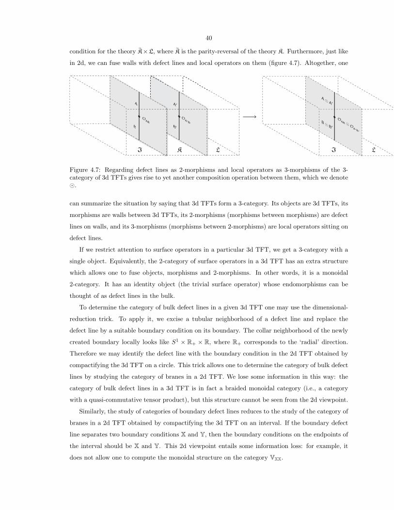
40

condition for the theory K×L, where K is the parity-reversal of the theory K. Furthermore, just like

in 2d, we can fuse walls with defect lines and local operators on them (figure 4.7). Altogether, one

Figure 4.7: Regarding defect lines as 2-morphisms and local operators as 3-morphisms of the 3-category of 3d TFTs gives rise to yet another composition operation between them, which we denote.

can summarize the situation by saying that 3d TFTs form a 3-category. Its objects are 3d TFTs, its

morphisms are walls between 3d TFTs, its 2-morphisms (morphisms between morphisms) are defect

lines on walls, and its 3-morphisms (morphisms between 2-morphisms) are local operators sitting on

defect lines.

If we restrict attention to surface operators in a particular 3d TFT, we get a 3-category with a

single object. Equivalently, the 2-category of surface operators in a 3d TFT has an extra structure

which allows one to fuse objects, morphisms and 2-morphisms. In other words, it is a monoidal

2-category. It has an identity object (the trivial surface operator) whose endomorphisms can be

thought of as defect lines in the bulk.

To determine the category of bulk defect lines in a given 3d TFT one may use the dimensional-

reduction trick. To apply it, we excise a tubular neighborhood of a defect line and replace the

defect line by a suitable boundary condition on its boundary. The collar neighborhood of the newly

created boundary locally looks like S1 × R+ × R, where R+ corresponds to the ‘radial’ direction.

Therefore we may identify the defect line with the boundary condition in the 2d TFT obtained by

compactifying the 3d TFT on a circle. This trick allows one to determine the category of bulk defect

lines by studying the category of branes in a 2d TFT. We lose some information in this way: the

category of bulk defect lines in a 3d TFT is in fact a braided monoidal category (i.e., a category

with a quasi-commutative tensor product), but this structure cannot be seen from the 2d viewpoint.

Similarly, the study of categories of boundary defect lines reduces to the study of the category of

branes in a 2d TFT obtained by compactifying the 3d TFT on an interval. If the boundary defect

line separates two boundary conditions X and Y, then the boundary conditions on the endpoints of

the interval should be X and Y. This 2d viewpoint entails some information loss: for example, it

does not allow one to compute the monoidal structure on the category VXX.

41

4.4 Four-dimensional TFT and 2-categories of surface oper-

ators

Boundary conditions in a 4d TFT form a 3-category. For example, if the 4d TFT is trivial, its

3-category of boundary conditions is the 3-category of all 3d TFTs. Similarly, walls (codimension-

1 defects) in a given 4d TFT form a monoidal 3-category. In this thesis we will avoid dealing

with such complicated structures and will focus instead on defects of codimension two, i.e., surface

operators in a 4d TFT. Such surface operators form a 2-category. One way to see it is to apply the

dimensional-reduction trick: excise a tubular neighborhood of a surface operator and replace the

operator by a suitable boundary condition on the newly created boundary. The collar neighborhood

of the boundary looks locally like S1 × R+ × R2, so we may reinterpret a surface operator as a

boundary condition in a 3d TFT obtained by compactifying the 4d theory on a circle. Then we can

appeal to the known fact that boundary conditions in a 3d TFT form a 2-category.

Of course, one can also explain the meaning of this 2-category structure directly in 4d terms.

The type of a surface operator may jump across a defect line, and one can regard defect lines on

surface operators as morphisms in a 2-category. Local operators sitting at a junction point of two

surface defect lines are 2-morphisms. The 4d viewpoint also makes it clear that the 2-category of

surface operators has a rich extra structure. First of all, one may fuse surface operators together

with defect lines and local operators sitting on them. This gives rise to a monoidal structure on the

2-category of surface operators. Second, by moving surface operators around one can easily see that

the fusion operation is quasi-commutative, i.e., one gets a braided monoidal 2-category.1

In this thesis, we will use the dimensional-reduction trick to study the 2-category of surface

operators of our twisted 4d TFTs in Chapter 6; we will not describe the braided monoidal structure

on this 2-category.

1A possible mathematical definition of a braided monoidal 2-category is spelled out in [34]. However, it appearsthat braided monoidal structures which arise in 4d TFT are of a rather special kind. In particular, the braiding isalways invertible.

42

Chapter 5

Compactifications of Vafa-Wittenand GL-twisted theories on a circle

We begin the project of compactifying the various twisted versions of N = 4, d = 4 SYM theory

to lower-dimensional TFTs, starting with the case of compactification to three dimensions on a

circle. Our aim is twofold: we wish to shed light on lower-dimensional TFTs (in particular, duality

relationships between 4d TFTs extend to duality relationships between their dimensionally reduced

versions); moreover, the lower-dimensional TFTs will help us understand aspects of the original 4d

TFTs.

For instance, according to the dimensional-reduction trick discussed in Chapter 4, boundary

conditions of the 3d theory obtained by compactifying on a circle will classify the spectrum of

surface operators in the original 4d theory (we put off an analysis of these boundary conditions until

the following chapter).

In the present chapter, we reduce the Vafa-Witten theory and the GL-twisted theories at t = i,

t = 1, and t = 0 to three dimensions on a circle. The resulting 3d TFTs will be turn out to be

topological, gauged sigma models: the reduction at t = i yields a gauged version of the Rozansky-

Witten model introduced in [14], while the reduction at t = 1 and t = 0 yield gauged versions of the

3d A-model TFT introduced in [6]; the Vafa-Witten theory is equivalent to the t = 0 theory when

compactified on a circle.

5.1 Compactification of topological gauge theories

Before turning to the S1 reductions in earnest, let us make a few general remarks about com-

pactification of topological gauge theories. Consider one of our 4d TFTs on the product manifold

M = W ×S1 where W is a Riemannian, oriented 3-manifold and S1 is a circle of circumference 2πR.

We wish to find an effective description in the R → 0 limit. (More generally, one can compactify

43

using a small compactification manifold of dimension two or higher.)

The usual Kaluza-Klein notion of compactification of a field theory is that one expands the fields

of the 4d theory in terms of their Fourier modes along the circle and, in the limit R → 0, discards

all but the constant modes due to the fact that they become infinitely massive. In this manner, one

obtains an effective 3d theory on W . (More precisely, one must integrate the nonzero modes out of

the path integral, which can induce quantum corrections in the effective theory.)

But a TFT does not ‘care’ about the size of R, in the sense that changes in R alter the action

by BRST-exact amounts and therefore leave topological correlators invariant. Hence (modulo the

subtleties we discuss in a moment) the reduced theory — though it describes a simplified region of

field space in which fields do not vary along the compact direction — is exactly equivalent to the

original theory. This convenient fact has been put to use in [1], where the GL-twisted theories at

t = i and t = 1 were given 2d descriptions by compactifying on 2d surfaces. We set the circumference

at the convenient value 2πR = 2π for the remainder of the chapter.

When our theory is a topological gauge theory, there are two important subtleties that compli-

cate this picture. The first is that a given field configuration on the product manifold may leave

some residual continuous gauge symmetry unbroken on the compactification manifold. Such field

configurations represent singular points in the target space of the effective sigma model description:

points where qualitatively new branches in the compactified theory open up. Practically, all one

can do is to excise such configurations ‘by hand’ (for instance, by imposing appropriate boundary

conditions that eliminate their occurrence). The 2d effective theories in [1] were truncated in just

this manner. This problem does not arise in the present context since our compactification manifold

is just S1.

The second subtlety, however, is important for our analysis. Consider first an abelian gauge

theory with gauge field A. It is not quite correct to simply declare A to be x4-independent and the

component A4 to be a real scalar field, where x4 is the coordinate for S1, ranging from x4 = 0 to

x4 = 2π. This is because the x4-dependent gauge transformation g(x4) = exp(imx4) shifts the value

of A4 by an integer amount:

A4 7→ A4 + im, m ∈ Z.

Hence, the 3d effective theory is ill-defined if written directly in terms of the scalar A4.

The solution to the problem is to write the effective theory instead in terms of the periodic scalar

h = exp(−2πA4)

which field is invariant with respect to x4-dependent gauge transformations.

For nonabelian gauge group, an extra complication is that requiring the fields of the 4d theory

to be independent of the x4 coordinate is not a gauge-invariant condition. One can try to avoid

44

dealing with this issue by first fixing a gauge such that A4 does not depend on x4, and, indeed, this

works in the neighborhood of A4 = 0, i.e., when the holonomy of A along S1 is close to unity. But

in general the condition that A4 is x4-independent does not fix the freedom to make x4-dependent

gauge transformations. For example, suppose A4 is proportional to an element µ ∈ g satisfying

exp(2πµ) = 1.

Such µ are precisely those which lie in the G-orbits of the cocharacter lattice of G. Then the gauge

transformation

g(x4) = exp(µx4)

shifts A4 by µ:

A4 7→ A4 + µ .

Such a gauge transformation in general makes other fields x4-dependent.

The solution again is to replace A4 in the description of the theory by a group-valued field h,

now defined to be the holonomy of A around the compact direction. Let us see how this works in

detail. In computing a particular correlator of the 4d theory via compactification, it is convenient to

first deform the support of all inserted operators to lie along the embedded hypersurface W0 ⊂ M ,

defined as the locus of points in W × S1 with x4 = 0. (Deforming in this manner does not affect

the value of the correlator due to topological invariance.) Next, we define the 3d field h to be the

holonomy of the connection around the loop beginning at a point (~x, 0) ∈ W0 and winding once

around the compact direction:

h(~x) = P exp(−∫ 2π

0

dx4A4(~x, x4))

for any ~x ∈W , where the holonomy is computed in the N -dimensional defining representation. Let

PW be the principal G bundle on W given by pulling back P under the embedding map

W −→W0 −→M

For nonabelian G, the holonomy h is no longer gauge invariant; rather, it is gauge covariant, trans-

forming as a section of the fiber bundle with typical fiber G associated to PW by the conjugation

action of G on itself; that is,

h ∈ Ω0(W, PW ×G G) .

In particular, h is a perfectly well-defined scalar field in three dimensions.

45

5.2 S1 compactification of Vafa-Witten theory

Consider first the Vafa-Witten theory placed on the product manifold M = W × S1. We will

show that, on this particular geometry for M , the theory is equivalent to a gauged version of the

3d A-model with target space X = g, where the gauge sector is a slight modification of the 3d

A-type gauge theory discussed in Section B.2.1 (by replacing the algebra-valued scalar field ς by a

group-valued field).

Reduced field content

We relabel the fields of the Vafa-Witten theory in a way that exposes the role they will play in the

3d reduced theory. In the following, the indices r, s, t = 1, 2, 3 refer to coordinates on W and the

superscript [VW ] indicates the corresponding field of the Vafa-Witten theory, as we have written in

Chapter 3. The 3d reduction of the field content will split into a gauge sector and a matter sector.

The 3d gauge sector will come from the relabeled fields:

Ar = A[VW ]r , λr = ψ[VW ]

r

ς = A[VW ]4 , ρ = ψ

[VW ]4

σ = σ[VW ],

σ = σ[VW ], ρ = η[VW ]

λr = χ[VW ]r4 , Hr = H

[VW ]r4 .

The 3d matter sector will come from the relabeled fields:

φ = φ[VW ], η = ζ [VW ]

br = B[VW ]r4 , ψr = ψ

[VW ]r4

β = χ[VW ]4 , P = H

[VW ]4

χr = χ[VW ]r , Pr = H [VW ]

r .

46

The BRST variations (3.8) of the Vafa-Witten theory, written in terms of the relabeled fields, become

δQA = λ, δQλ = −dAσ,

δς = ρ, δQρ = [σ, ς]

δQσ = 0,

δQσ = ρ, δQρ = [σ, σ]

δQλ = H, δQH = [σ, λ]

δQφ = η, δQη = [σ, φ]

δQb = ψ, δQψ = [σ, b]

δQβ = P, δQP = [σ, β]

δQχ = P , δQP = [σ, χ] .

(5.1)

If we were to naıvely reduce to 3d by keeping only the constant Fourier modes of the above fields,

then we would have the correct field content and variations for a gauged 3d A-model TFT with target

space g (parameterized by the field φ), as written in Section B.2. However, as we have discussed

above, the field A4 is ill-defined as a 3d scalar field, and must be replaced by its holonomy h in the

description of the theory. Moreover, we must also replace its BRST partner ρ by an appropriately

averaged field. We define

ρ = − 1

2π

∫ 2π

0

dx4H−1ρH

where

H(x4) = P exp(−∫ x4

0

dtA4

)is the holonomy of A along the arc of the circle from 0 to x4, so that, in particular H(2π) = h. One

can then verify, after some work, that the BRST-variations of h and ρ are given by

h−1δQh = 2πρ

δQ(hρ) = (2π)−1[σ, h] .

Combining these, one confirms that δ2Qh = [σ, h], i.e., a gauge transformation with parameter σ.

The field ρ transforms as a section

ρ ∈ Ω0(W,adPW ) .

47

Reduced action

In order to write out the Vafa-Witten action in terms of the relabeled fields, it is helpful to use the

following identities. Let χµν and Fµν be 2-forms in 4d and let

νr = χr4, νr = (∗χ)r4

ωr = Fr4, ωr = (∗F )r4

be the 1-forms in 3d given by restricting F , ∗F , χ, and ∗χ to the 1,2,3 directions, where * indicates

the 4d Hodge dual. We have

√g(

12χµνF

µν)

=√g44√gW

(νr ω

r + νr ωr)

where gµν is the 4d metric with determinant g and (gW )rs is the 3d metric with determinant gW .

In a similar vein, we have

Frs =√g44√gW εrstω

t =√g44(? ω)rs

where ? is the 3d Hodge star. Finally, let Bµν be a self-dual 2-form in 4d and let Cµν be the following

2-form appearing in the Vafa-Witten localization equations:

Cµν = 12gρτ [Bµρ, Bντ ]

One finds that

Cr4 = (∗C)r4 = 12

√g44√gW εrst[b

s, bt] = 12

√g44(? [b, b]

)r

where br = Br4. For our choice of the circle circumference, g44 = g44 = 1.

The Vafa-Witten action (3.9), written in terms of the relabeled fields, becomes:

S =

∫M

d4x√g(L1 + L2 + L3 + L4

)− iτ

4π

∫M

TrF ∧ F

where

L1 =1

e2δQ Tr

4λr(Hr −DrA4 + ∂4Ar − (?F )r

)+ 2σ d?Aλ

L2 =

1

e2δQTr

χr(Pr − 2Drφ+ 2

(? dAb

)r

)+ β

(P − 2d?Ab

)L3 =

1

e2δQTr

4λr(− [br, φ] + 1

2 ? [b, b]r

)+ 2χrD4br − 2βD4φ

L4 =

1

e2δQTr

2σ(− [ψr, b

r]− [η, φ]− 12 [σ, ρ] +D4 ρ

)(5.2)

where d?Aλ = Drλr. Simply keeping constant modes in the above action would result in a 3d action

48

containing commutator terms of the form, e.g.,

[A4, φ]

which (as we have been stressing) would not be well defined due to the explicit appearance of A4. In

order to eliminate the appearance of A4, we exploit the wide freedom of choice available in writing

down the action for a given cohomological TFT. Namely, we are free to continuously deform the

BRST-exact portion of the action in any way without affecting the values of topological correlators,

provided that the bosonic kinetic terms remain well defined, and that we do not alter the field

content or variations of the theory. We write down a new action S by replacing the commutator

[A4, φ] inside the BRST-exact portion of S with

(2π)−1(Adh−1φ− φ

)= −(2π)−1h−1[h, φ] .

(The latter expression reduces to the former in the neighborhood of A4 ≈ 0.) One can smoothly

interpolate between S and S with a family of actions

Sα = (1− α)S + αS

for 0 ≤ α ≤ 1 such that, as we dial the parameter α from zero to one, the action is smoothly deformed

by a BRST-exact amount. (The effect of nonzero α is to ‘turn on’ higher-order BRST-exact terms

involving A4 commutators.) At α = 1, we are left with the equivalent action S, which, it should

be emphasized, is not Lorentz-invariant due to the appearance of h. Unlike S, the action S can be

safely be reduced to 3d by requiring fields to be independent of the x4 coordinate, and one obtains

S =

∫W

d3x√gW

(L1 + L2 + L3 + L4

)+ Stop

where

L1 =1

e2δQ Tr

4λr(Hr + (2π)−1h−1Drh− ?Fr

)+ 2σ d?Aλ

L2 =

1

e2δQTr

χr(Pr − 2Drφ+ 2

(? dAb

)r

)+ β

(P − 2d?Ab

)L3 =

1

e2δQTr

4λr(− [br, φ] + ?[b, b]r

)− 2(2π)−1χrh−1[h, br] + 2(2π)−1β h−1[h, φ]

L4 =

1

e2δQTr

− 2σ

([λr, b

r] + [η, φ]− 12 [ρ, σ] + (2π)−1h−1[h, ρ ]

)(5.3)

and Stop is the coupling-dependent term measuring the 4d instanton number in the 4d action. After

acting with δQ, one finds that the kinetic term of the bosonic field h takes the standard form for a

49

group manifold sigma model map:

Trh−1(Drh)h−1 (Drh)

where the metric on G is taken to be the left-invariant metric induced by Tr at the identity.

After the integrating out the auxiliary fields, one finds that the theory localizes on the BPS

equations

F − (2π)−1h−1 ? dAh+ [?b, φ]− [b, b] = 0

?dAb− dAφ− (2π)−1h−1[h, b] = 0

d?Ab− (2π)−1h−1[h, φ] = 0

(5.4)

as well as equations involving σ.

The above field content, action and variations are those of a gauged 3d A-model with target

g. The gauge sector is not precisely the 3d A-type gauge theory as described in Section B.2.1 but,

rather, a modification in which the Lie algebra valued scalar field ς is replaced by a Lie group valued

field h.

Instanton term

We wish to interpret the instanton term in the above action in 3d terms. The analysis splits into

two cases: when G = U(1) and when G is simple.

In case G = U(1), we write the reduction of the instanton term as

Stop = − iτ2

∫W

F ∧ dA4 (5.5)

Note that it is the periodicity of A4 that makes this topological term nontrivial in general.

In case G is simple, there are no such deformation terms available for measuring the topological

class of the principal bundle on W . In fact, since we have taken W to be compact, the term automat-

ically vanishes. More generally, we wish to consider the possibility of inserting disorder operators

and allowing W to have boundaries. For instance, in Chapter 6, we will describe the 2-category of

surface operators of the 4d theory as the 2-category of 3d boundary conditions. However, the lack

of 3d deformations demonstrates that anything about the theory understandable in purely 3d terms

will be τ -independent; e.g., the 2-categorical structure of surface operators. As we have mentioned

in Chapter 4, this 2-category secretly possesses a braided, monoidal structure (corresponding to

colliding surface operators), which extra structure could be dependent on τ . But, since we will not

be examining the braided monoidal structure, we discard the instanton term from the action of the

3d compactified theory.

50

5.3 S1 compactification of GL-twisted theory at t = 0

We turn now to the reduction of the GL-twisted theories, treating first the case t = 0. The analysis

will proceed similarly for each value of t. The Vafa-Witten theory and the t = 0 theory turn out to

reduce to the same theory in three dimensions.

The fact that the Vafa-Witten twisted theory and t = 0 are identical on the manifold W ×S1 can

be understood as follows. Recall from Section 2.4.1 that, after performing the Vafa-Witten twist of

N = 4, d = 4 SYM, the scalar supercharge Q is drawn from amongst the left-handed Q’s. On the

other hand, performing the GL-twist also results in a left-handed scalar supercharge Ql precisely

when t = 0; indeed, it can be taken to be the same one. The Vafa-Witten and t = 0 theories then

only differ in how fields transform under the 4d rotation group; e.g., the Vafa-Witten theory has

a self-dual 2-form Bµν and 0-form φ, while the t = 0 theory has a 1-form φµ. However, the fields

transform identically under the the 3d rotation subgroup; e.g., both 3d reduced theories have a 3d

1-form br and a 3d 0-form φ.

Explicitly, recall from Section 2.5.2 the action for the GL-twisted theory at t = 0:

S =

∫M

d4x√g(L1 + L2

)− τ

4πi

∫M

TrF ∧ F

where

L1 =1

e2δQTr

χµνH

µν − 2χ+µν

(F − 1

2 [φ, φ])µν

+ 2χ−µν(dAφ

)µνL2 =

1

e2δQTr

− η(P − 2d∗Aφ

)+ σ

(2d∗Aψ + 2[ψµ, φ

µ] + [σ, η])

.

(5.6)

We relabel the fields of the GL-twisted theory in 3d terms as follows (the superscript [0] indicates

the corresponding field of the GL-twisted theory at t = 0, as we have written in Chapter 2). The

gauge sector fields are

Ar = A[0]r , λr = iψ[0]

r

ς = A[0]4 , ρ = iψ

[0]4

σ = −iσ[0],

σ = −iσ[0], ρ = η[0]

λr = χ+[0]r4 , Hr = H

+[0]r4

The matter sector fields are

φ = −φ[0]4 , η = iψ

[0]4 ,

br = −φ[0]r , ψr = iψ[0]

r

β = η[0], P = −P [0]

χr = 2χ−[0]r4 , Pr = 2H

−[0]r4 .

It is easily verified that the BRST variations of the relabeled fields are given by (5.1) above.

51

If one exchanges A4 for its holonomy h, ρ for ρ (as we have done for the Vafa-Witten theory)

and reduce to three dimensions, then the 3d reduced action matches that (5.3) of the reduction of

Vafa-Witten theory, except for the sign of the term

1

e2δQTr4λr[br, φ]

which changes the sign of the term [?b, φ] in (5.4). However, solutions to the BPS equations set this

term to zero anyway, so this sign is irrelevant and we conclude that the reductions of the Vafa-Witten

and t = 0 theories are identical.

5.4 S1 compactification of GL-twisted theory at t = 1

The reduction of the t = 1 theory again yields a gauged version of the 3d A-model. There are,

however, a few important differences as compared with the Vafa-Witten and t = 0 reductions. The

field A4 will now lie in the matter sector (instead of the gauge sector) of the 3d theory; indeed,

the target space of the reduced theory will be the group G, parameterized by the holonomy h.

Accordingly, the matter sector fields take values in the vector space ThG rather than g ' T1G.

Moreover, the coefficient of the topological term in the action is just θ instead of the complexified

coupling τ , implying that we can avoid the complications of interpreting the instanton term by setting

θ = 0. Lastly, the gauge sector will be a conventional 3d A-type gauge theory, as described in Section

B.2.1 (rather than an exotic version involving a group-valued scalar).

The action for the GL-twisted theory [1] at t = 1 is given by

S =

∫M

d4x√g(L1 + L2

)+

iθ

8π2

∫M

TrF ∧ F

where

L1 =1

e2δQTr

χµν

(12H − F + 1

2 [φ, φ]− ∗dAφ)µν

L2 =1

e2δQTr

− η(P − 2d∗Aφ

)+ σ

(2d∗Aψ + 2[ψµ, φ

µ] + [σ, η])

.

(5.7)

Relabeling the fields, we have the gauge sector fields

Ar = A[1]r , λr = i

(ψ[1]r + ψ[1]

r

)ς = φ

[1]4 , ρ = i

(ψ

[1]4 − ψ

[1]4

)σ = −2iσ[1],

σ = −2iσ[1], ρ = 2(η[1] + η[1]

),

λr =(∗ χ)[1]

r4, Hr =

(∗H

)[1]

r4,

52

and the matter sector fields

φ = A[1]4 , η = i

(ψ

[1]4 + ψ

[1]4

),

br = φ[1]r , ψr = i

(ψ[1]r − ψ[1]

r

),

β = 12

(η[1] − η[1]

), P = P [1] ,

χr = χ[1]r4 , Pr = H

[1]r4 .

The BRST variations of the relabeled fields, once again, are given by (5.1). Writing out the t = 1

action in terms of the relabeled fields, we find

S =

∫M

d4x√g(L1 + L2 + L3 + L4 + L5

)where

L1 =1

e2δQ Tr

λr(Hr − 2Drς − 2 ? Fr

)+ 1

2 σ d?Aλ

L2 =1

e2δQTr

χr(Pr − 2DrA4 − 2

(? dAb

)r

)+ β

(P − 2d?Ab

)L3 =

1

e2δQTr

λr(

2D4br + ?[b, b]r

)+ χr

(2[br, ς] + 2∂4Ar

)L4 =

1

e2δQTr

2β(−D4ς − 1

8 [σ, σ])− 1

2 ρ(

12P − d

?Ab−D4ς + 1

8 [σ, σ])

L5 =1

e2δQTr

12 σ(d?Aψ +D4η +D4ρ+ [λr, b

r]− [ψr, br] + [η, ς]− [ρ, ς]

).

(5.8)

We again replace A4 in the description of the theory by its holonomy h. The target space is the

group manifold X = G, with sigma model map Φ given by the holonomy

Φ = h : W → G .

The 3d A-model fields η, br, β, P, χr, Pr now take values in ThG instead of the Lie algebra itself and it

is convenient to replace them by g-valued averages, exactly as we have done for ρ in the Vafa-Witten

reduction above, i.e.,

η ≡ − 1

2π

∫ 2π

0

dx4H−1ηH

and similarly for the other matter fields. The BRST variations of the averaged fields pick up an

extra term (due to the curvature of the group manifold), as follows:

δQbr = ψr+ < η, br >

δQχr =P r+ < η, χr >

53

where we have defined

< η, br > ≡∫ 2π

0

dx4[η, H−1brH

] ∣∣∣x4,

< η, χr > ≡∫ 2π

0

dx4η, H−1χrH

∣∣∣x4.

The reduction procedure will be similar to that which we have described for reducing the Vafa-

Witten action above: we smoothly deform the action by a BRST-exact amount to eliminate the

appearance of A4 in favor of h and the ThG-valued matter fields by their g-valued averages. After

reducing to 3d, one obtains

S =

∫W

d3x√gW

(L1 + L2 + L3 + L4 + L5

)where

L1 =1

e2δQ Tr

λr(Hr − 2Drς − 2 ? Fr

)+ 1

2 σ d?Aλ

L2 =1

e2δQTr

χr(P r + 2(2π)−1h−1Drh− 2

(? dAb

)r

)+ β

(P − 2d?Ab

)L3 =

1

e2δQTr

λr(− 2(2π)−1h−1[h, br] + ?[b, b]r

)+ 2χr [br, ς]

L4 =

1

e2δQTr

2β(

(2π)−1h−1[h, ς]− 18 [σ, σ]

)− 1

2 ρ(

12 P − d

?Ab+ (2π)−1h−1[h, ς] + 1

8 [σ, σ])

L5 =1

e2δQTr

12 σ(d?Aψ − (2π)−1h−1[h, η]− (2π)−1h−1[h, ρ] + [λr, b

r]− [ψr, br] + [η, ς]− [ρ, ς]

).

After integrating out the auxiliary fields, one finds that the theory localizes on the BPS equations

F + ?dAς − 12 [b, b] + (2π)−1h−1[h, ?b] = 0

?dAb− [b, ς]− (2π)−1h−1Drh = 0

d?Ab− (2π)−1h−1[h, ς] = 0 .

We have obtained a gauged 3d A-model with target space G. This 3d TFT has not been much

studied in the literature, but, as it is conjectured to be dual to the 3d reduction of the t = i theory,

a study of its properties is expected to yield many interesting mathematical predictions. In the

subsequent chapter we will take a modest first step in this direction by analyzing its 2-category of

boundary conditions for the case G = U(1).

54

5.5 S1 compactification of GL-twisted theory at t = i

The reduction of the GL-twisted theory at t = i can be analyzed in a similar way; however, the

resulting 3d reduced theory will have a very different character to the cases considered so far. One

obtains a gauged version of a well-studied 3d TFT, the Rozansky-Witten (RW) model [14], [36].

(The gauging is accomplished by coupling to a 3d B-type gauge theory, as described in Section B.4.)

The target space of the model is the cotangent bundle of the complexified Lie group, X = T ∗GC,

equipped with the conjugation action of G on the base GC, as well as the induced action on the

fibers. This comes about as follows.

The BRST-invariant, complex fields σ and A4 + iφ4 of the t = i theory will descend to the matter

sector of the 3d theory. As we have discussed, the field A4 itself is not well-defined and must be

exchanged for an appropriate group-valued scalar. We define

hC = P exp(−∫ 2π

0

dx4(A4 + iφ4))

taking values in the associated bundle with fiber GC

hC ∈ Ω0(W, PW ×G GC) .

Its conjugate is

hC = P exp(−∫ 2π

0

dx4(A4 − iφ4)).

The field hC is a good coordinate for the base and σ is a good coordinate for the fiber of T ∗GC.

The manifold T ∗GC turns out to endowed with a hyperkahler metric [63], although it is nontrivial

to describe explicitly.

Simply declaring the target to be T ∗GC obscures an important symmetry of the action. For

a general hyperkahler target space X, the RW model has a Z2 ghost number symmetry, but, as

explained in [36], when X is a cotangent bundle one can promote it to a U(1) ghost number symmetry

by letting the fiber coordinates have ghost number two. This accords nicely with the fact that σ

has ghost number two already in the 4d theory. Hence, to emphasize that the fiber coordinate is

formally assigned ghost number two we will denote the target manifold instead by T ∗[2]GC.

The action of the GL-twisted theory at t = i is written in (2.4). The relabelings of the fields

are as follows (adopting the convention that a ‘[i]’ superscript denotes fields of the t = i theory, and

55

r, s, t = 1, 2, 3 refers to W coordinates). For the 3d gauge sector, we have

Ar = A[i]r ,

ϕr = φ[i]r ,

Ar = (Ar + iφr)[i]

Ar = (Ar − iφr)[i]

λr = i(ψr + iψr

)[i]

,

ζrs = −i(χ+ − iχ−

)[i]rs,

ρ =1√2

(ψ4 − iψ4

)[i]

,

ρ =1

2(η − iη)

[i].

and for the matter sector we have

σ =√

2σ[i],

τ = (A4 + iφ4)[i],

ησ =√

2i (η + iη)[i],

ητ = 2i(ψ4 + iψ4

)[i]

,

χσr =1√2

(ψr − iψr

)[i]

,

χτr =(χ+ − iχ−

)[i]r4

.

In addition, it is useful to introduce an auxiliary 0-form P in order to make the BRST variations

nilpotent off-shell; P -dependent terms in the action are chosen to ensure that its equation of motion

is

P = d?Aϕ−i

2([σ, σ] + [τ , τ ]) .

56

The BRST variations of the relabeled fields are given by

δQA = λ, δQσ = 0,

δQϕ = iλ, δQτ = 0,

δQλ = 0, δQσ = ησ

δQζ = −iF , δQτ = ητ

δQρ = [τ, σ], δQησ = 0,

δQρ = iP, δQητ = 0,

δQP = 0, δQχσ = dAσ,

δQχτ = dAτ.

where dA is the covariant derivative and F curvature with respect to complexified connection A.

The action written in terms of the relabeled fields is given by

S =

∫M

d4x√g (L1 + L2 + L3) + Stop

where

L1 = − 1

2e2δQ Tr

i2ζrsF

rs + iρ(P − 2d?A ϕ+ i[σ, σ] + i[τ , τ ]

)L2 = − 1

2e2δQ Tr

χτr (dAτ)r + χσr (dAσ)r

L3 = − 1

2e2δQ Tr

ρ [τ , σ]

,

Stop =

√2

e2

∫W

Triχτ ∧ dAχσ − ζ ∧

(dA ρ+ [χσ, τ ]− [χτ , σ]

).

After replacing τ by hC, certain matter fields are tangent to a nonidentity point of the (complexified)

group and it is convenient to replace them by algebra-valued averages in the description of the theory

(just as for the t = 1 reduction above). Namely, ητ (taking values in ThC) and χτ (taking values in

ThC) are exchanged for averaged fields

η τ ≡ − 1

2π

∫ 2π

0

dx4H−1

C ητ HC

χ τ ≡ − 1

2π

∫ 2π

0

dx4H−1C χτ HC .

57

The BRST variations written in terms of the new variables are as follows

δQhC = 0

δQhC = 2π hC ητ

δQχτ = (2π)−1h−1

C dAhC

δQητ = 0 .

The reduction proceeds similarly to what we have done for the Vafa-Witten, t = 0, and t = 1

theories: we deform the action by a BRST-exact amount to write it in terms of the new variables

and then reduce to 3d by taking fields to be independent of the x4 coordinate. The resulting 3d

action is given by

S =

∫W

d3x√gW (L1 + L2 + L3) + Stop

where

L1 = − 1

2e2δQ Tr

i2ζrsF

rs + iρ(P − 2d?A ϕ+ i[σ, σ] + i[τ , τ ] + . . .

)L2 = − 1

2e2δQ Tr

− (2π)−1χ τr h

−1

C (dAhC)r + χσr (dAσ)r

L3 = − 1

2e2δQ Tr

− (2π)−1ρ h

−1

C [hC, σ],

where the . . . in L1 indicate higher-order terms that we do not write explicitly. The G-invariant

symplectic form on the target space is proportional to

Ω = Tr dσ h−1C dhC.

The G-invariant Kahler form on the target space corresponds to the hyperkahler metric described

in [63] and does not admit a simple closed-form expression; in a neighborhood of the identity it is

proportional to

J =i

2Tr(dσdσ + dτdτ

).

The moment maps µ3, µ+, µ− of the G-action with respect to symplectic forms J , Ω, and Ω are

proportional to the following functions of the coordinates:

µ3 = − i2

([σ, σ] + [τ , τ ] + . . . )

µ+ = −ih−1C [hC, σ]

µ− = −ih−1

C [hC, σ] .

We have shown that the BRST-exact portion of the action and variations reduce to those of a

58

gauged Rozansky-Witten model with target T ∗[2]GC written in Section B.5. We conjecture that the

topological term Stop also reduces appropriately to the topological term of this model (although we

do not show this here).

59

Chapter 6

Surface operators of 4d TFTs

Having written down the twisted versions of N = 4 SYM and analyzed their 3d reductions, we

are in a position to classify the spectrum of surface operators in these theories. As emphasized in

Chapter 4, the surface operators of a given 4d TFT have the structure of a 2-category; namely, the

2-category of boundary conditions of the 3d reduced TFT.

In this chapter, we systematically employ this observation to classify surface operators of the

GL-twisted theories at t = i, t = 1, and t = 0. (By what we have said in the preceding chapter, the

Vafa-Witten theory will have the same spectrum of surface operators as that of the t = 0 theory.)

The advantage of the 3d viewpoint is that the problem of classifying boundary conditions is more

familiar.

The material in this chapter was presented in [4]. Much of the analysis of boundary conditions

of the reduced theories relies on work on 2d and 3d TFTs relegated to the appendices A and B.

6.1 Gukov-Witten surface operators

The simplest surface operators of the GL-twisted theories have been introduced by S. Gukov and

E. Witten [2]. They are disorder operators corresponding to a codimension-2 singularity in the gauge

field A and bosonic 1-form φ of the form

A = αdθ, φ = βdr

r− γdθ.

Here α is an element of a maximal torus T of G, and β, γ are elements of the Lie algebra t of T.

For simplicity, let us assume that the triple (α, β, γ) breaks G down to T. Gauge transformations

which preserve T form the Weyl group W; the triplet (α, β, γ) is defined up to the action of W on

T× t× t. All fields other than A and φ are nonsingular.

The surface operator depends on an additional parameter η taking values in the torus Hom(Λcochar, U(1)).

Here Λcochar is the lattice of magnetic charges Hom(U(1),T). Equivalently, as explained in [2], η can

60

be thought of as taking values in LT, the maximal torus of the Langlands-dual group. The parameter

η arises as follows. First, note that the above singularity in the fields breaks the gauge group down

to T. Thus if D is the codimension-2 submanifold on which the surface operator is supported, the

restriction of the gauge field to D has a first Chern class c1|D taking values in Λcochar. Given η we

can insert into the path-integral a phase factor

η(c1(D)).

This factor depends only on the behavior of the gauge field on D and can be regarded as an η-

dependent modification of the surface operator defined above.

Gukov-Witten surface operators are BRST-invariant for arbitrary t, but their properties depend

on t. We will see below that there are many other surface operators. In what follows we will focus

on the cases t = i, t = 1, and t = 0. The first two cases are exchanged by S-duality (at zero θ-angle)

and play a prominent role in the physical approach to the geometric Langlands program [1]. The

last case is self-dual and is the most natural starting point for understanding quantum geometric

Langlands duality [35].

We shall find that, for each value of t, there exist much more general surface operators.

6.2 Surface operators at t = i and G = U(1)

In Section 5.5, we found that the t = i theory on W × S1 reduces to a gauged Rozansky-Witten

model on W with target T ∗GC. Initially, we take G = U(1) and analyze boundary conditions of

the gauged RW model with target T ∗C∗. The analysis of boundary conditions splits cleanly into

boundary conditions of the matter sector and boundary conditions of the gauge sector; we discuss

each in turn.

6.2.1 Boundary conditions of RW model, target T ∗C∗

According to [36] the simplest boundary conditions in the RW model correspond to complex La-

grangian submanifolds of X. If we want to preserve ghost number symmetry, these Lagrangian

submanifolds must be invariant with respect to the rescaling σ 7→ λ2σ, λ ∈ C∗. This requires the

Lagrangian submanifold of T ∗C∗ to be the conormal bundle of a complex submanifold in C∗. This

means that a (closed) C∗-invariant complex Lagrangian submanifold is either the zero section σ = 0

or one of the fibers of the cotangent bundle given by τ = τ0. The zero section boundary condition

plays a special role and will be denoted X0 in this subsection.

More general boundary conditions correspond to families of B-models or Landau-Ginzburg mod-

els parameterized by points in a complex Lagrangian submanifold. As mentioned in [36] and ex-

61

plained in more detail in [37] it is sufficient to restrict oneself to the case when the Lagrangian

submanifold is the zero section σ = 0. One can describe these boundary conditions more alge-

braically as follows. Recall that the category of boundary line operators on the boundary X0 is a

monoidal category which we denote VX0X0. Given any boundary condition X one may consider the

category VXX0of boundary defect lines which may separate X from X0. This category is a mod-

ule category over the monoidal category VX0X0. It was proposed in [36] that this module category

completely characterizes the boundary condition X. Concretely, in the case of the RW model with

target T ∗[2]C∗ the category of boundary line operators VX0X0is equivalent to Db(Coh(C∗)). One

way to see it is to reduce the RW model on an interval with the boundary condition X0 on both

boundaries. The resulting 2d TFT is a B-model with target C∗, and its category of branes may

be identified with Db(Coh(C∗)). The 2d viewpoint does not allow one to determine the monoidal

structure, but one can show that it is given by the usual derived tensor product [36, 37].

It was further argued in [36, 37] that the 2-category of boundary conditions for the RW model

with target T ∗[2]C∗ is equivalent to the derived 2-category of module categories over Db(Coh(C∗)).

That is, it is the 2-category of derived categorical sheaves over C∗ as defined by B. Toen and

G. Vezzosi [44]. This provides an algebraic description of boundary line operators and their OPEs

for all boundary conditions.

6.2.2 Boundary conditions of B-type 3d gauge theory, G = U(1)

Recall from Section 5.5 that the bosonic fields A|W , φ|W and the fermionic fields ψ + iψ, χ, η −

iη, ψ4− iψ4 reduce correctly to fields of the B-type 3d gauge theory (discussed in Section B.4), with

action given by

S = − 1

2e2δQ

∫W

(χ ∧ ?F − i

2(η − iη) ∧ ?d?φ

)+

1

2e2

∫W

(ψ4 − iψ4)dχ

In principle we should gauge-fix the theory and modify the BRST operator appropriately, but

throughout this thesis we suppress this complication.

As in any gauge theory, the most natural boundary conditions are the Dirichlet and Neumann

ones. The Dirichlet condition requires the restriction of A + iφ to the boundary to be trivial. In

addition, one requires φ3 (the component of φ orthogonal to the boundary) to satisfy the Neumann

condition ∂3φ3 = 0. BRST-invariance then fixes the boundary conditions for fermions: the restriction

of the forms ψ + iψ, χ and η − iη to the boundary must vanish, The Neumann boundary condition

leaves the restriction of A to the boundary unconstrained but requires the restriction of the 1-form

?F = ?dA to vanish. In addition φ3 must satisfy the Dirichlet boundary condition, i.e., it must take

a prescribed value on the boundary. In the Neumann case BRST-invariance requires the restrictions

of the fermions ?χ, ψ3 + iψ3 and ψ4− iψ4 to vanish. Note that in the Dirichlet case the gauge group

62

is completely broken at the boundary, while in the Neumann case it is unbroken.

The Dirichlet condition does not have any parameters, while the Neumann condition seems to

depend on a single real parameter β, the boundary value of φ3. On the quantum level there is

another parameter: we can add to the action a boundary topological term

θ

∫∂W

F2π

In fact, both parameters are irrelevant, in the sense that topological correlators do not depend on

them. The irrelevance of the parameter θ follows from the fact that the above topological term is

BRST-exact and equal toθ

2πδQ

∫∂W

χ

To see the irrelevance of the parameter β, note that to shift β we need to add to the action a

boundary term proportional to ∫∂W

∂3φ3

Since φ1 and φ2 vanish on the boundary, this is also BRST-exact and proportional to

δQ

∫∂W

(η − iη).

Following the same line of thought as in [36], one can try to describe the 2-category of boundary

conditions in this theory by picking a distinguished boundary condition X0 and characterizing any

other boundary condition X by the category VXX0 of defect line operators between X and X0. That

is, one attaches to any boundary condition X a module category VXX0 over the monoidal category

VX0X0.

An obvious guess for the distinguished boundary condition is the free (Neumann) one since it

leaves the gauge group unbroken. To determine the category of boundary line operators VX0X0 for

this boundary condition, one may reduce the 3d theory on an interval and study the category of

branes in the resulting 2d TFT. In the Neumann case, reduction on an interval gives the following

result: the bosonic fields are the gauge field A and the 1-form φ, the fermionic ones are the 0-form

η − iη, the 1-form ψ + iψ and the 2-form χ. This is the field content of a B-type topological gauge

theory in 2d, see Section A.2. It is easy to check that the BRST transformations of these fields

are also the same as in the B-type 2d gauge theory. The category of branes for this 2d TFT is the

category of graded finite-dimensional representations of G = U(1), see Section A.2 for details. This

is because the only boundary degrees of freedom one can attach are described by a vector space

which carries a representation of the gauge group. The monoidal structure cannot be determined

from 2d considerations, but it easy to see that it is given by the usual tensor product. Indeed, as

described in Section A.2, a brane corresponding to a representation space V is obtained by inserting

63

the holonomy of the complex connection A = A+ iφ in the representation V into the path-integral.

From the 3d viewpoint this means that the corresponding boundary line operator is the Wilson line

operator for A in the representation V . On the classical level, the fusion of two Wilson line operators

in representations V1 and V2 gives the Wilson line in representation V1 ⊗ V2, and clearly there can

be no quantum corrections to this result (the gauge coupling e2 is an irrelevant parameter).

To summarize, the monoidal category VX0X0is the category of graded finite-dimensional repre-

sentations of C∗, or equivalently the equivariant derived category of coherent sheaves over a point

which we denote DbC∗(Coh(•)). We propose that the 2-category of boundary conditions is equivalent

to the 2-category of module categories over DbC∗(Coh(•)). To give a concrete class of examples of

such a module category, consider a Calabi-Yau manifold Y with a C∗ action. The corresponding B-

model can be coupled to the boundary gauge field and provides a natural set of topological boundary

degrees of freedom for the 3d gauge theory. The corresponding category of boundary-changing line

operators is the C∗-equivariant bounded derived category of Y which is obviously a module category

over DbC∗(Coh(•)).

6.2.3 Putting the sectors together

It is fairly obvious how to combine boundary conditions for the two models. The most basic boundary

condition in the full theory is σ = 0 in the RW sector and the free (Neumann) condition in the gauge

sector. We will call this the distinguished boundary condition. The bosonic fields which are free on

the boundary are the C∗-valued scalar h = exp(−2πτ) and the restriction of the complex gauge field

A = A+ iφ. More general boundary conditions involve a boundary B-model or a boundary Landau-

Ginzburg model fibered over C∗ and admitting a C∗-action. The fibration over C∗ determines the

coupling to the boundary value of τ , while the C∗-action determines the coupling to the boundary

gauge field A.

As in the RW model, we can give a more algebraic definition of the set of all boundary conditions

in the full theory. This description is also useful because it suggests how to define the 2-category

structure of the set of boundary conditions. We consider the monoidal category of boundary line

operators for the distinguished boundary condition. This is the category of branes for the 2d TFT

obtained by reducing the gauged RW model on an interval. Since the reduction of the B-type 3d

gauge theory gives the B-type 2d gauge theory, and the reduction of the RW model gives the B-model

with target C∗, the effective 2d TFT is the gauged B-model with target C∗, where the gauge group

U(1) acts trivially. As described in Section A.3, the corresponding category of branes is equivalent

to DbC∗(Coh(C∗)). The monoidal structure cannot be determined from the 2d considerations, but

it is easy to see (given the results for the RW model and the B-type gauge theory in 3d) that it is

given by the derived tensor product.

Every boundary condition gives rise to a module category over this monoidal category. It is

64

natural to conjecture that the converse is also true, i.e., every reasonable module category over this

monoidal category can be thought of as a boundary condition for the full 3d TFT. For example, we

may consider a family of Calabi-Yau manifolds parameterized by points of C∗ such that each model

in the family has a C∗ symmetry. The corresponding module category is the C∗-equivariant derived

category of the total space of the fibration. This gives us a conjectural description of the 2-category

of surface operators in the parent 4d gauge theory.

Let us describe how Gukov-Witten surface operators fit into this picture. Such operators depend

on a complex parameter h0 = exp(−2π(α − iγ)) taking values in C∗. From the 3d viewpoint, h0

determines the boundary value of the scalar h = exp(−2πτ) in the RW sector. The other scalar σ is

left free. Thus the boundary conditions for the RW sector correspond to a Lagrangian submanifold

of T ∗[2]C∗ given by h = h0 (the fiber over the point h0). The gauge sector boundary conditions

are of Neumann type and have no nontrivial parameters.There are no boundary degrees of freedom.

From our algebraic viewpoint we may describe this as follows. In the usual RW theory the fiber

over h = h0 corresponds to a skyscraper sheaf of DG-categories over C∗ whose ‘stalk’ over h0 is

the category of bounded complexes of vector spaces. We may denote it Db(Coh(•)). Including

the gauge degrees of freedom means working with a sheaf of categories with a C∗ action. Thus

we simply consider a skyscraper sheaf of categories over C∗ whose ‘stalk’ over h0 is the category of

C∗-equivariant complexes of vector spaces DbC∗(Coh(•)). The monoidal category Db

C∗(Coh(C∗)) acts

on it in a fairly obvious manner: one simply tensors an object of DbC∗(Coh(•)) with the (derived)

restriction of an object of DbC∗(Coh(C∗)) to the point h = h0.

6.2.4 Line operators on Gukov-Witten surface operators

The category of morphisms between two different skyscraper sheaves of categories is trivial (the set

of objects is empty). This corresponds to the fact that two different Gukov-Witten surface operators

cannot join along a boundary-changing line operator. But the category of line operators sitting on a

particular Gukov-Witten surface operator (i.e., the endomorphism category of a Gukov-Witten sur-

face operator) is nontrivial. Its most obvious objects are Wilson lines for the complexified gauge field

A, which are obviously BRST-invariant. Such operators are labeled by irreducible representations

of C∗. One might guess therefore that the category of surface line operators is simply the category

of representations of C∗, or perhaps the category of C∗-equivariant complexes of vector spaces which

we denoted DbC∗(Coh(•)) above. However, this naive guess is wrong, which can be seen by inspecting

BRST-invariant local operators which can be inserted into such a Wilson line operator. From the

abstract viewpoint they form an algebra (the endomorphism algebra of an object in the category

of line operators). It is clear that any power of the field σ gives such an operator, so the algebra

of local operators on a line operator is the algebra of polynomial functions of a single variable of

ghost number 2. In what follows we will denote the line parameterized by σ by C[2] to indicate that

65

σ sits in degree 2; thus C[2] is a purely even graded manifold. On the other hand, the algebra of

endomorphisms of an irreducible representation of C∗ is simply C.

To determine what the category of line operators is it is convenient to take the 2d viewpoint and

reduce the 3d theory on an interval with the Gukov-Witten-type boundary condition on both ends.

Let x3 denote the coordinate on the interval. Gukov-Witten boundary conditions eliminate the

complex scalar h (which is now locked at the value h0) and the field φ3 but keep the complex scalar

σ and the gauge field A. Thus the effective 2d theory also has two sectors: the B-model with target

C[2] and the B-type 2d topological gauge theory. According to A.3, the corresponding category of

branes is equivalent to the C∗-equivariant derived category of C[2]: its objects can be regarded as

C∗-equivariant complexes of holomorphic vector bundles on C[2] (with a trivial C∗ action on C[2]).

This answer is independent of the parameter h0 = exp(−2π(α−iγ)) of the Gukov-Witten surface

operator. In particular, we can choose the trivial surface operator h0 = 1, in which case we should

get the category of bulk line operators in the GL-twisted theory at t = i.

It is not difficult to see that this answer for the category of bulk line operators agrees with the

computation of the endomorphism algebra of a Wilson line explained above. Indeed, an insertion

of a Wilson line does not put any constraints on σ and does not add any degrees of freedom, and

therefore should correspond to a trivial line bundle over C[2]. Its fiber carries a representation of

C∗ determined by the charge of the Wilson line. The endomorphism algebra of such an object of

DbC∗(Coh(C[2])) is simply the algebra of polynomial functions on C[2].

It is now clear that the category of line operators contains objects other than Wilson lines. For

example, we may consider a skyscraper sheaf at the origin of C[2], whose stalk at the origin is a

complex line V carrying some representation of C∗. There are two different ways to define the

corresponding line operator. First, we may consider a free resolution of the skyscraper:

V [−2]⊗O→V ⊗O,

where V [−2] means V placed in ghost degree −2, O is the algebra of polynomial functions on C[2],

and the cochain map is multiplication by σ. The shift by −2 is needed so that the cochain map

has total degree 1. The existence of such a resolution means that we can realize the ‘skyscraper’

line operator as a ‘bound state’ of two Wilson lines both associated with the representation V but

placed in different cohomological degrees. The corresponding bulk line operator is obtained using

the formulas of Section A.3, where the target of the gauged B-model is taken to be C[2], the vector

bundle E on C[2] is trivial and of rank 2, with graded components in degrees 1 and 0, and the bundle

morphism T from the former to the latter component is multiplication by σ. In accordance with the

66

results of Section A.3, we consider a superconnection on σ∗E of the form

N =

nA 0

12 (ψ − iψ) nA

,

where n ∈ Z is the weight with which C∗ acts on V . The bulk line operator corresponding to the

skyscraper sheaf at the origin of C[2] is the holonomy of this superconnection along the insertion

line `.

Another (equivalent) way is to take seriously the fact that the skyscraper sheaf is localized at

σ = 0 and require the field σ to vanish at the insertion line `. To make this well defined, one needs to

excise a small tubular neighborhood of ` and impose a suitable boundary condition on the resulting

boundary. This condition must set σ = 0 and leave the components of A tangent to the boundary

` unconstrained. BRST-invariance determines uniquely the boundary conditions for all other fields.

6.3 Surface operators at t = i and G nonabelian

It was shown in Section 5.5 that compactification of the t = i theory for general G yields a gauged

Rozansky-Witten model with target T ∗[2]GC (the ‘[2]’ indicates that the fiber coordinates of the

cotangent bundle are formally assigned ghost number 2). The G-action on T ∗[2]GC is induced by

the conjugation action on the base.

6.3.1 Some simple boundary conditions

Let us consider some boundary conditions in the gauged Rozansky-Witten model with target

T ∗[2]GC. The most natural boundary condition in the gauge sector is the Neumann condition,

which preserves full gauge-invariance on the boundary. In the matter sector one has to pick a G-

invariant complex Lagrangian submanifold of T ∗[2]GC which is invariant with respect to the rescaling

of the fiber. Such a Lagrangian submanifold can be constructed by picking a GC-invariant closed

complex submanifold of GC and taking its conormal bundle. For example, one can take the whole

GC, and then the Lagrangian submanifold is given by σ = 0. We will call the resulting boundary

condition in the gauged RW model the distinguished boundary condition. It is an analogue of the

NN condition in the abelian case.

Another natural choice of a G-invariant Lagrangian submanifold is the conormal bundle of a

complex conjugacy class in GC. In order for the submanifold to be closed take the conjugacy class

to be semisimple. This boundary condition is a nonabelian analogue of the ND condition. The

corresponding surface operator is a semisimple Gukov-Witten-type surface operator. Indeed, fixing

a semisimple conjugacy class of exp(−2π(A4+iφ4)) is the same as fixing a semisimple conjugacy class

67

of the limiting holonomy of the complex connection A+ iφ in the 4d gauge theory. More generally,

if the conjugacy class is not closed, one needs to consider the conormal bundle of its closure.

It is easy to analyze boundary line operators for these boundary conditions. Reducing the 3d

theory on an interval with the distinguished boundary conditions we get a B-type 2d gauge theory

coupled to a B-model with target GC. The gauge group acts on GC by conjugation. According to

A.3, the corresponding category of branes is equivalent to DbGC

(Coh(GC)). The monoidal structure

cannot be deduced from the 2d considerations, but the same analysis as in the usual RW model

shows that it is given by the derived tensor product.

In the Gukov-Witten case we need to fix a semisimple complex conjugacy class C in GC. Let N∗C

denote the total space of its conormal bundle in T ∗GC. Concretely, it is the space of pairs (g, σ),

where g ∈ C and σ ∈ gC satisfies Trσ g−1δg = 0 for any δg tangent to C at g. The fiber coordinate

σ has cohomological degree 2; to indicate this we will denote the corresponding graded complex

manifold N∗[2]C. Reduction on an interval in the Gukov-Witten case gives a B-type 2d gauge

theory coupled to a B-model whose target is N∗[2]C. Its category of branes is DbGC

(Coh(N∗[2]C)).

The monoidal structure is given by the derived tensor product.

6.3.2 Bulk line operators

It is interesting to consider the special case of a Gukov-Witten surface operator corresponding to the

trivial conjugacy class in GC (i.e., the identity). This is the trivial surface operator, so the category

of 3d boundary line operators in this case can be identified with the category of bulk line operators

in the 4d TFT. The conormal bundle of the identity element is simply the dual of the complexified

Lie algebra gC; the group GC acts on it by the adjoint representation. Thus the category of 4d bulk

line operators is equivalent to DbGC

(Coh(g∗C[2])). In other words, it is the GC-equivariant derived

category of the graded algebra ⊕pSympg where the pth component sits in cohomological degree 2p.

In view of this result it is interesting to consider local operators sitting at the junction of

two Wilson loops in representations V1 and V2 of G. The corresponding objects of the category

DbGC

(Coh(g∗C[2])) are free modules over A = ⊕pSympg[2] of the form V1 ⊗C A and V2 ⊗ A, with

the obvious GC action. The space of morphisms between them is the space of GC-invariants in the

infinite-dimensional graded representation

V ∗1 ⊗ V2 ⊗ A .

Indeed, a BRST-invariant and gauge-invariant junction of two Wilson lines should be an operator

in representation V ∗1 ⊗ V2 constructed out of the complex scalar σ taking values in gC. The space

of such operators in ghost number 2p is HomG(Sympg, V ∗1 ⊗ V2), where HomG denotes the space of

morphisms in the category of representations of G. Summing over all p we get the above answer.

68

6.3.3 More general surface operators

As in the abelian case, the above examples do not exhaust the set of objects in the 2-category of

surface operators. For example, in [47] more complicated surface operators have been considered

which involve higher-order poles for the complex connection A = A + iφ. By analogy with the

Rozansky-Witten model we propose that the most general surface operator at t = i (or equivalently,

the most general boundary condition in the 3d theory) can be defined as a module category of

the monoidal category of boundary line operators for the distinguished boundary condition X0. As

explained above, this monoidal category is DbGC

(Coh(GC)). Concretely, this means that the most

general surface operator can be obtained by fibering a family of 2d TFTs over GC, so that the GC

action on the base (by conjugation) lifts to a GC action on the whole family. For example, one

may consider a complex manifolds X which is a fibration over GC, so that fibers are Calabi-Yau

manifolds, and one is given a lift of the GC action on the base (by conjugation) to a GC action on

the total space.

Given any surface operator X, one may construct a module category over DbGC

(Coh(GC)) by

looking at the category of line operators sitting at the junction of X and the distinguished surface

operator X0. This category is the category of branes in the 2d TFT obtained by compactifying the 3d

TFT on an interval, with the boundary conditions on the two ends given by X and X0. Equivalently,

one may compactify the 4d TFT on a twice-punctured 2-sphere, with surface operators X and X0

inserted at the two punctures.

For example, if we consider a surface operator defined, as in [47], by a prescribed singularity in

the complex connection A, and take into account that the distinguished surface operator is defined

by allowing the holonomy of A to be free, we see that the space of vacua of the effective 2d TFT is

the moduli space of connections on a punctured disc with the prescribed singularity at the origin.

Let us denote this moduli space M. If in the definition of M we divide by the group of gauge

transformations which reduce to the identity at some chosen point on the boundary of the disk, then

M is acted upon by GC and is fibered over GC (the holonomy of A along the boundary of the disk).

It looks plausible that the effective 2d TFT is the B-model with targetM coupled to a B-type gauge

theory with gauge group GC. Its category of branes is a module category over DbGC

(Coh(GC)).

6.4 Surface operators at t = 1 and G = U(1)

In Section 5.4, we found that, for t = 1, the GL-twisted theory compactifies to a gauged 3d A-model

TFT with target space G. The analysis of the boundary conditions of the matter sector (a 3d A-

model with target G, see Section B.1) has been carried out in [6]. However, boundary conditions of

the full gauged 3d A-model have not previously been analyzed. In this section, we restrict ourselves

to G = U(1), in which case the gauge sector splits cleanly from the matter sector.

69

6.4.1 Boundary conditions in the gauge sector

The gauge sector is the dimensional reduction of the Donaldson-Witten 4d TFT [45] down to 3d; in

Appendix B we call this the A-type 3d gauge theory. However, this by itself does not teach us very

much, since boundary conditions in this theory have not been discussed previously. Without adding

boundary degrees of freedom, the only choices are the Dirichlet and Neumann boundary conditions

for gauge fields, with BRST-invariance fixing the conditions on all other fields.

6.4.1.1 The Dirichlet condition

Let us begin with the Dirichlet condition which says that the restriction of A to the boundary is

trivial. Since δ2Q = 2iδg(σ), this makes sense only if σ also vanishes on the boundary. BRST-

invariance then requires η + η and the restriction of the 1-form ψ + ψ to vanish. The fermionic

equations of motion then require the restriction of χ to vanish, and the BRST-invariance implies

that φ4 must satisfy the Neumann condition ∂3φ4 = 0, where we assumed that the boundary is given

by x3 = 0.

The Dirichlet boundary condition has the property that it has no nontrivial local BRST-invariant

boundary observables. Indeed, the only nonvanishing BRST-invariant 0-form is ψ4 − ψ4, but it is

BRST-exact. To analyze boundary line operators, we use the dimensional reduction trick and

compactify the 3d theory on an interval with the Dirichlet boundary conditions. The only bosonic

fields in the effective 2d theory are the constant mode of φ4 and the holonomy of A along the interval

parameterized by x3. That is, the bosonic fields are a real scalar and a periodic real scalar. The

effective 2d TFT is therefore a sigma-model with target R × S1. In fact, it can be regarded as an

A-model with target T ∗S1. The easiest way to see this is to note that the path-integral of the 3d

theory localizes on configurations given by solutions of the Bogomolny equations

F + ?dφ4 = 0.

Upon setting all fields to zero except A3 and φ4 and assuming that they are independent of x3, this

equation becomes

dA3 + ?dφ4 = 0,

where ? is the 2d the Hodge star operator. This is an elliptic equation which can be interpreted as

the holomorphic instanton equation, provided we declare A3 + iφ4 to be a complex coordinate on

the target. Since the action of the 4d theory is BRST-exact, so is the action of the 2d model. This

agrees with the well-known fact that the action of an A-model is BRST-exact if the symplectic form

on the target space is exact.

The category of line operators on the Dirichlet boundary is therefore the Fukaya-Floer category

70

of T ∗S1 whose simplest objects are Lagrangian submanifolds equipped with unitary vector bundles

with flat connections. Since this category arises as the endomorphism category of an object in a

2-category, it must have a monoidal structure, which is not visible from the purely 2d viewpoint. In

fact, we do not expect the Fukaya-Floer category of a general symplectic manifold to have a natural

monoidal structure. We will argue below that the monoidal structure is induced by the mirror

symmetry which establishes the equivalence of the Fukaya-Floer category of T ∗S1 with Db(Coh(C∗))

and the monoidal structure on the latter category. For now we just note that the base S1 has a

distinguished point corresponding to the trivial holonomy of A on the interval. The fiber over this

point is a Lagrangian submanifold in T ∗S1 and is the identity object with respect to the monoidal

structure. The distinguished point allows us to identity S1 with the group manifold U(1).

6.4.1.2 The Neumann condition

Now let us consider the Neumann condition for the 3d gauge field A. This means that the gauge

symmetry is unbroken on the boundary and the restriction of the 1-form ?F vanishes. Then the

Bogomolny equation requires φ4 to have the Dirichlet boundary condition φ4 = a = const, and by

BRST-invariance ψ4 − ψ4 must vanish at x3 = 0. Fermionic equations of motion imply then that

ψ3 + ψ3 vanishes as well, and since δQ(ψ3 + ψ3) = 2∂3σ, the field σ satisfies the Neumann condition.

Finally, the restriction of the 1-form ?χ to the boundary must vanish, in order for the fermionic

boundary conditions to be consistent. Indeed, if x1 is regarded as the time direction, then (?χ)2 is

canonically conjugate to ψ3 + ψ3, so if one of them vanishes, so should the other. Similarly, if x2 is

regarded as time, then (?χ)1 is canonically conjugate to ψ3 + ψ3 and therefore must vanish too.

In the Neumann case the space of BRST-invariant local observables on the boundary is spanned

by powers of the field σ. To determine the category of boundary line operators one has to reduce

the 3d gauge theory on an interval with the Neumann boundary conditions. The bosonic fields of

the effective 2d theory are the 2d gauge field and the constant mode of the scalar σ, the fermionic

ones are the 0-form η + η, the 1-form ψ + ψ, and the 2-form χ. Their BRST transformations are

δQA = i(ψ + ψ),

δQσ = 0,

δQσ = i(η + η),

δQ(η + η) = 0,

δQ(ψ + ψ) = 2dσ,

δQχ = F.

This 2d TFT can be obtained from the usual N = (2, 2) d = 2 supersymmetric gauge theory by

71

means of a twist which makes use of the U(1)V R-symmetry. Since this is the same R-symmetry as

that used for constructing an A-type sigma-model, we might call this TFT an A-type 2d gauge theory.

As far as we know, its boundary conditions have not been analyzed in the literature previously. It

is shown in Section A.1 that its category of branes is equivalent to the bounded derived category

of coherent sheaves on the graded line C[2]. 1 Again, the 3d origin of this category means that it

must have monoidal structure. Here it is given by the usual derived tensor product of complexes of

coherent sheaves. The trivial line bundle on C[2] is the identity object. From the 3d viewpoint, it

corresponds to the ‘invisible’ line operator on the boundary.

As mentioned above, the Neumann condition depends on a real parameter a, the boundary value

of the scalar φ4. On the quantum level there is another parameter which takes values in R/2πZ. It

enters as the coefficient of a topological term in the boundary action:

θ

∫x3=0

F

2π.

Thus overall the Neumann condition in the gauge sector has the parameter space R× S1 ' C∗.

6.4.2 Boundary conditions in the matter sector

We may impose either Dirichlet or Neumann condition on the periodic scalar A4. Let us discuss

these two possibilities in turn.

6.4.2.1 The Dirichlet condition

If A4 satisfies the Dirichlet condition, then BRST-invariance requires the 1-form φ to satisfy the

Neumann condition. This means that the components of φ tangent to the boundary are free and

satisfy ∂3φ1 = ∂3φ2 = 0, while the component φ3 takes a fixed value φ3 = a on the boundary.

BRST-invariance also requires the following fermions to vanish on the boundary: ψ4 + ψ4, ψ3 − ψ3,

ρ1, ρ2. The real parameter a together with the boundary value of A4 combine into a parameter

taking values in S1 × R. These parameters are actually irrelevant, in the sense that topological

correlators do not depend on them. To see this, note that shifting the boundary value of A4 can be

achieved by adding a boundary term to the action of the form

∫x3=0

∂3A4d2x =

∫x3=0

(δQρ3 − (∂1φ2 − ∂2φ1)) d2x .

We see that up to a total derivative this boundary term is BRST-exact, hence does not affect the

correlators. A similar argument can be made for the boundary value of φ3.

Placing the theory on W = Σ×I (with Σ a 2-manifold and I an interval with Dirichlet boundary

1This category is equivalent to the U(1)-equivariant constructible derived category of sheaves over a point [28].

72

conditions) yields a novel 2d TFT on Σ that we shall call the modified A-model in Chapter 7 (where

we will study its properties at greater length). For a target space X equipped with a U(1) action,

one can twist the ordinary 2d A-model to produce a modified A-model with target X. In our case,

X = C, endowed with rotations by a phase. The bosonic C-valued field Z of the ordinary A-model

becomes, after twisting, a real 1-form (the two components are the real and imaginary components

of Z). This is the 1-form φ|Σ that survives reduction.

Apart from the bosonic 1-form φ, the modified A-model has a fermionic 1-form ψ− ψ and a pair

of fermionic 0-forms η − η and ρ (the latter comes from the component ρ3 of the 1-form ρ in 3d).

Their BRST transformations are

δQφ = i(ψ − ψ),

δQ(ψ − ψ) = 0,

δQ(η − η) = 2d?φ,

δQρ = ?dφ .

Here ? is the 2d Hodge star operator, and d? = ?d?.

To understand the category of boundary line operators in 3d, we need to describe the category

of boundary conditions for the modified A-model. This is fairly straightforward. A natural class of

boundary conditions is obtained by imposing on the boundary

(aφ+ b ? φ) |∂W = 0.

The special cases b = 0 and a = 0 correspond to the 2d Dirichlet and Neumann conditions. Since

the theory obviously has a symmetry rotating φ into ?φ, it is sufficient to consider the Neumann

condition ?φ| = 0. BRST-invariance requires the restriction of ?ψ and ρ to vanish on such a

boundary. It is easy to see that there are no nontrivial BRST-invariant boundary observables (the

only BRST-invariant fermion ψ is BRST-exact), so there is no possibility to couple boundary degrees

of freedom in a nontrivial way. This implies that the category of boundary conditions is the same

as for a trivial 2d TFT, i.e., the category of complexes of finite-dimensional vector spaces. We may

denote it Db(Coh(•)).

There is an important subtlety here related to the fact that the scalar A4 is periodic with period

1. When reducing on an interval, this means that there are ‘winding sectors’, where

∫dx3∂3A4 = n, n ∈ Z.

This winding is constant along a connected component of the boundary and does not affect the 2d

73

theory in any way. We may incorporate it by introducing an additional integer label on each bound-

ary component which serves as a conserved boundary charge. This is mathematically equivalent to

saying that the category of boundary conditions is the category of C∗-equivariant coherent sheaves

over a point DbC∗(Coh(•)). Objects of this category are complexes of finite-dimensional vector spaces

with a C∗-action, such that the differentials in the complex commute with the C∗ action. Morphisms

are required to preserve the C∗-action, i.e., to have zero C∗-charge.

6.4.2.2 The Neumann condition

If A4 satisfies the Neumann condition ∂3A4 = 0, then BRST-invariance requires φ to satisfy the

Dirichlet condition . That is, the restriction of φ to the boundary must vanish, and φ3 must satisfy

∂3φ3 = 0. This boundary condition does not have any parameters.

The reduction on an interval gives rise to the A-model with the bosonic fields A4 and φ3. This

can be seen, for example, by looking at the 3d BPS equation dA4 + ?dφ = 0 and restricting to field

configurations where φ1 = φ2 = 0 and A4 and φ3 are independent of x3. For such field configuration

the BPS equation becomes the holomorphic instanton equation with target S1 ×R ' C∗. From the

symplectic viewpoint, C∗ with its standard Kahler form is isomorphic to T ∗S1. Thus the category

of boundary line operators in this case is the Fukaya-Floer category of T ∗S1. Since this category

arises as the category of boundary line operators in the 3d TFT, it must have a monoidal structure.

Although the category appears to be the same as in the gauge sector with the Dirichlet boundary

condition, we will see that the monoidal structure is completely different and is induced by the

equivalence between (a version of) the Fukaya-Floer category of T ∗S1 and the constructible derived

category of S1 [43]. In particular, the identity object (i.e., the invisible boundary line operator)

is different and corresponds to the zero section of T ∗S1 with a trivial rank-1 local system. This

illustrates the fact that a monoidal structure on branes in a 2d TFT depends on the way this 2d

TFT is realized as a compactification of a 3d TFT on an interval.

6.4.3 Electric-magnetic duality of surface operators at t = i and t = 1

We are now ready to describe how the 4d electric-magnetic duality acts on various boundary con-

ditions described above. Since for both gauge and matter sectors one can have either Dirichlet or

Neumann conditions, there are four possibilities to consider.

From the 3d viewpoint, 4d electric-magnetic duality amounts to dualizing the 3d gauge field A

into a periodic scalar, and simultaneously dualizing the periodic scalar A4 into a 3d gauge field. It

is easy to see that electric-magnetic duality applied to the A-type gauge theory gives the Rozansky-

Witten model with target T ∗[2]C∗, i.e., it maps the A-type gauge sector to the B-type matter sector.

Similarly, it maps the A-type matter sector into the B-type gauge theory (with gauge group U(1)).

In other words, electric-magnetic duality reduces to particle-vortex duality done twice.

74

The dual of the Neumann condition for a periodic scalar is the Dirichlet condition for the gauge

field, and vice versa. We will use this well-known fact repeatedly in what follows.

6.4.3.1 The DD condition

The first possibility is the Dirichlet condition in both gauge and matter sectors at t = 1. The

Dirichlet condition in the A-type gauge sector maps into a boundary condition in the Rozansky-

Witten model with target T ∗[2]C∗ which sets σ = 0 on the boundary and leaves the complex scalar

τ free to fluctuate. The Dirichlet condition in the A-type matter sector is mapped to the Neumann

condition in the B-type gauge theory. Note that the Dirichlet condition in the A-type matter sector

has two real parameters taking values in S1 and R. The former one is mapped to a boundary

theta-angle, i.e., a boundary term in the action of the form

θ

∫x3=0

F

2π= θ

∫x3=0

F2π.

The latter parameter is the boundary value of the field φ3. Both of these parameters are irrelevant,

as discussed in section 4.

As discussed above, the category of boundary line operators in the A-type 3d gauge theory is the

Fukaya-Floer category of T ∗U(1). On the other hand, the category of boundary line operators in

the Rozansky-Witten model is Db(Coh(C∗)), as explained in [36]. These categories are equivalent,

by the usual 2d mirror symmetry.

Let us recall how 2d mirror symmetry acts on some objects in this case. The trivial line bundle on

C∗ is mapped to the fiber over a distinguished point of the base S1. This distinguished point allows

us to identify S1 with the group manifold U(1). More generally, we may consider a holomorphic line

bundle on C∗ with a ∂-connection of the form

∂ + iλdz

z, λ ∈ C.

We will denote such a line bundle Lλ. Gauge transformations can be used to eliminate the imaginary

part of λ. They also can shift the real part of λ by an arbitrary integer. Thus we may regard the

parameter λ as taking values in R/Z ' S1. Mirror symmetry maps Lλ to a Lagrangian submanifold

in T ∗U(1) which is a fiber over the point exp(2πiλ) ∈ U(1).

Applying mirror symmetry to the obvious monoidal structure on Db(Coh(C∗)) given by the

derived tensor product we get a monoidal structure on the Fukaya category of T ∗U(1). The trivial

holomorphic line bundle on C∗, which serves as the identity object in Db(Coh(C∗)), is mapped to

the Lagrangian fiber over the identity element of U(1). If we consider two Lagrangian fibers over

the points exp(2πiλ1), exp(2πiλ2) ∈ U(1), their mirrors are line bundles Lλ1 and Lλ2 . Their tensor

75

product is a line bundle Lλ1+λ2whose mirror is the Lagrangian fiber over the point exp(2πi(λ1 +

λ2)) ∈ U(1). Clearly, this rule for tensoring objects of the Fukaya category makes use of the group

structure of U(1), i.e., it is a convolution-type tensor product.

Another natural class of Lagrangian submanifolds to consider are constant sections of T ∗U(1),

i.e., submanifolds given by the equation φ4 = const. These submanifolds are circles and may carry a

nontrivial flat connection. Thus such A-branes are labeled by points of R× U(1) ' C∗. The mirror

objects are skyscraper sheaves on C∗. The derived tensor product of two skyscrapers supported at

different points is obviously the zero object. The derived tensor product of a skyscraper with itself

can be shown to be isomorphic to the sum of the skyscraper and the skyscraper shifted by −1. That

is, it is a skyscraper sheaf over the same point whose stalk is a graded vector space C[−1] ⊕ C.

Applying mirror symmetry, we see that the tensor product of a section of T ∗U(1) with itself must

be the sum of two copies of the same section, but with the Maslov grading of one of them shifted

by −1. We do not know how to reproduce this result without appealing to mirror symmetry, i.e.,

by computing the product of boundary line operators in the A-type gauge theory.

As discussed above, the category of boundary line operators in the A-type matter sector is the

category of branes in a somewhat unusual 2d TFT which is a modification of the A-model with

target T ∗R. It was argued above that this category is equivalent to DbC∗(Coh(•)). This agrees with

the B-side, where the reduction on an interval gives a B-type 2d gauge theory.

Putting the gauge and matter sectors together, we see that the DD boundary condition on the A-

side is mapped to what we called the distinguished boundary condition on the B-side. The category

of boundary line operators for such a boundary condition is the C∗-equivariant derived category

of coherent sheaves DbC∗(Coh(C∗)) with its obvious monoidal structure. On the A-side we get a

graded version of the Fukaya-Floer category of T ∗U(1) where a flat vector bundle over a Lagrangian

submanifold has an additional integer grading and morphisms are required to have degree zero with

respect to it. This grading arises from the winding number of the periodic scalar A4.

We can also interpret the duality in 4d terms. Indeed, it is easy to see that the DD boundary

condition on the A-side arises from a 4d Dirichlet boundary condition at t = 1, while its dual on

the B-side arises from the 4d Neumann condition at t = i. Thus electric-magnetic duality exchanges

Dirichlet and Neumann boundary conditions in 4d, as expected. The surface operators corresponding

to such 4d boundary conditions can be interpreted as follows: we excise a tubular neighborhood of

the support of the surface operator and impose the 4d boundary condition on the resulting boundary.

In a TFT, such a procedure gives a surface operator (i.e., there is no need to take the limit where

the thickness of the tubular neighborhood goes to zero).

76

6.4.3.2 The NN condition

This condition is the distinguished boundary condition on the A-side, since the gauge group is

unbroken on the boundary, and the periodic scalar A4 is free to explore the whole circle. It is

mapped by electric-magnetic duality to the Dirichlet boundary condition for the B-type gauge theory

and the boundary condition in the RW model with target C∗ which fixes the C∗-valued scalar τ

and leaves σ free. Note that both the Neumann boundary condition in the A-type gauge theory

and the corresponding boundary condition in the RW model have a parameter taking values in

C∗ ' R× U(1).

Let us compare the categories of boundary line operators. The category of boundary line opera-

tors in the A-type gauge theory is the bounded derived category of coherent sheaves Db(Coh(C[2])).

The category of boundary line operators in the RW model is also Db(Coh(C[2])). The category of

boundary line operators in the A-type matter sector is the Fukaya-Floer category of T ∗S1. The

category of boundary line operators in the B-type gauge sector is Db(Coh(C∗)). Their equivalence

is a special case of the usual 2d mirror symmetry.

But there is more: we expect that the categories of boundary line operators are equivalent as

monoidal categories. This is easy to see directly for the RW model with target C∗ and A-type gauge

theory with gauge group U(1). Indeed, in both cases typical objects in the category of boundary

line operators are complexes of holomorphic vector bundles which can be represented by Wilson

line operators on the boundary for some superconnection on the pullback vector bundle. In the

classical approximation, fusing two such boundary line operators corresponds to the tensor product

of complexes, and there can be no quantum corrections to this result.

It is more complicated to compare the monoidal structures for the other pair of dual theories

(B-type gauge theory and A-type matter). We will not attempt to do an independent computation

on the A-side but instead describe the monoidal structure on the B-side and then explain what it

corresponds to on the A-side.

Note that since C∗ is a complex Lie group, the category Db(Coh(C∗)) has two natural monoidal

structures: the derived tensor product, and the convolution-type product. The former one does not

make use of the group structure, while the latter one does. The identity object of the former one is

the sheaf of holomorphic functions on C∗, while for the latter structure it is the skyscraper sheaf at

the identity point 1 ∈ C∗. It is the latter monoidal structure which describes the fusion of boundary

line operators on the B-side. Indeed, the 3d meaning of the coordinate on C∗ is the holonomy of

the connection A+ iφ along a small semicircle with both ends on the boundary and centered at the

boundary line operator (see figure 6.1). Skyscraper sheaves correspond to boundary line operators

for which this holonomy is fixed. In particular, the skyscraper sheaf at 1 ∈ C∗ corresponds to the

‘invisible’ boundary line operator for which this holonomy is trivial. By definition, this is the identity

object in the monoidal category of boundary line operators.

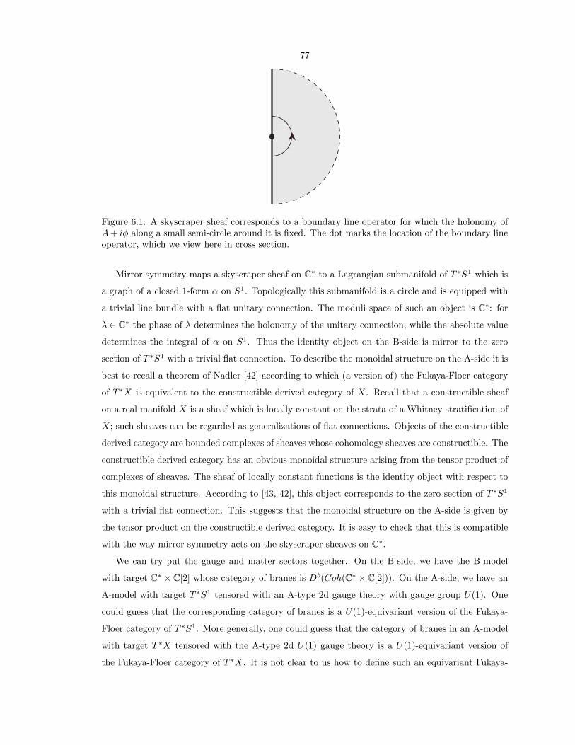
77

Figure 6.1: A skyscraper sheaf corresponds to a boundary line operator for which the holonomy ofA+ iφ along a small semi-circle around it is fixed. The dot marks the location of the boundary lineoperator, which we view here in cross section.

Mirror symmetry maps a skyscraper sheaf on C∗ to a Lagrangian submanifold of T ∗S1 which is

a graph of a closed 1-form α on S1. Topologically this submanifold is a circle and is equipped with

a trivial line bundle with a flat unitary connection. The moduli space of such an object is C∗: for

λ ∈ C∗ the phase of λ determines the holonomy of the unitary connection, while the absolute value

determines the integral of α on S1. Thus the identity object on the B-side is mirror to the zero

section of T ∗S1 with a trivial flat connection. To describe the monoidal structure on the A-side it is

best to recall a theorem of Nadler [42] according to which (a version of) the Fukaya-Floer category

of T ∗X is equivalent to the constructible derived category of X. Recall that a constructible sheaf

on a real manifold X is a sheaf which is locally constant on the strata of a Whitney stratification of

X; such sheaves can be regarded as generalizations of flat connections. Objects of the constructible

derived category are bounded complexes of sheaves whose cohomology sheaves are constructible. The

constructible derived category has an obvious monoidal structure arising from the tensor product of

complexes of sheaves. The sheaf of locally constant functions is the identity object with respect to

this monoidal structure. According to [43, 42], this object corresponds to the zero section of T ∗S1

with a trivial flat connection. This suggests that the monoidal structure on the A-side is given by

the tensor product on the constructible derived category. It is easy to check that this is compatible

with the way mirror symmetry acts on the skyscraper sheaves on C∗.

We can try put the gauge and matter sectors together. On the B-side, we have the B-model

with target C∗ × C[2] whose category of branes is Db(Coh(C∗ × C[2])). On the A-side, we have an

A-model with target T ∗S1 tensored with an A-type 2d gauge theory with gauge group U(1). One

could guess that the corresponding category of branes is a U(1)-equivariant version of the Fukaya-

Floer category of T ∗S1. More generally, one could guess that the category of branes in an A-model

with target T ∗X tensored with the A-type 2d U(1) gauge theory is a U(1)-equivariant version of

the Fukaya-Floer category of T ∗X. It is not clear to us how to define such an equivariant Fukaya-

78

Floer category mathematically. Given the results of [43, 42], a natural guess is the equivariant

constructible derived category of sheaves on X. As a check, note that when X is a point, the U(1)-

equivariant constructible derived category is equivalent to Db(Coh(C[2])) [28]. As mentioned above

and explained in Appendix A, this is indeed the category of branes for the A-type 2d gauge theory.

The monoidal structure seems to be the standard one (derived tensor product). On the B-side, on

the other hand, the monoidal structure is a combination of the tensor product of coherent sheaves

on C[2] and the convolution product on C∗.

6.4.3.3 The DN condition

Next consider the boundary condition on the A-side which is a combination of the Dirichlet condition

in the gauge sector and the Neumann condition for A4 in the matter sector. It is dual to the

Dirichlet condition for the B-type gauge sector and a boundary condition for the RW model with

target T ∗[2]C∗ which sets σ = 0 and leaves the complex scalar τ = A4 + iφ4 free to fluctuate.

On the B-side reduction on an interval gives a B-model with target C∗×C∗, therefore the category

of boundary line operators is Db(Coh(C∗ × C∗)). On the A-side reduction gives an A-model with

target T ∗U(1) × T ∗U(1), therefore the category of boundary line operators is the Fukaya-Floer

category. The two categories are equivalent by the usual 2d mirror symmetry. The monoidal

structure is easiest to determine on the B-side. It is neither the derived tensor product, nor the

convolution, but a combination of both. This happens because the two copies of C∗ have a very

different origin: one of them arises from a 3d B-type gauge theory, and the other one arises from

the Rozansky-Witten model with target T ∗[2]C∗.

6.4.3.4 The ND condition

Finally we consider the boundary condition on the A-side which is a combination of the Neumann

condition in the gauge sector and the Dirichlet condition for A4. This is the case which corresponds

to the Gukov-Witten surface operator at t = 1. Indeed, the Dirichlet conditions for A4, φ4 and φ3

mean that the holonomy of A is fixed, while the 1-form φ has a singularity of the form

βdr

r− γdθ,

where −γ is the boundary value of φ4 and β is the boundary value of φ3. The boundary value of A4

is the Gukov-Witten parameter α. The Neumann condition in the gauge sector also depends on the

boundary theta-angle which corresponds to the Gukov-Witten parameter η. As explained above,

the boundary values of A4 and φ3 are actually irrelevant. This agrees with the results of [2], where

it is shown that at t = 1 the parameters α and β are irrelevant. Thus the true parameter space of

the surface operator on the A-side is C∗.

79

Electric-magnetic duality maps the DD condition to the Neumann condition for the B-type gauge

theory and the boundary condition in the RW model which fixes τ and leaves σ free to fluctuate.

The latter boundary condition depends on the boundary value of the field τ = A4 + iφ4. From the

4d viewpoint this boundary value encodes the Gukov-Witten parameters α and γ. These are the

relevant parameters at t = i, as explained in [2]. The Neumann boundary condition in the B-type

gauge theory also has two parameters (the boundary value of φ3 and the boundary theta-angle)

which correspond to the Gukov-Witten parameters β and η. But as explained above and from a

different viewpoint in [2], these parameters are irrelevant at t = i.

Let us compare the categories of 3d boundary line operators, which from the 4d viewpoint are

interpreted as categories of line operators sitting on Gukov-Witten surface operators. On the B-side

reduction on an interval gives a B-model with target C[2] tensored with a B-type 2d gauge theory,

therefore the category of boundary line operators is DbC∗(Coh(C[2])). On the A-side reduction on

an interval gives an A-type 2d gauge theory tensored with a modified A-model with target T ∗R. Its

category of branes is a modification of the category of boundary conditions for the A-type 2d gauge

theory where the space of boundary degrees of freedom has additional integer grading coming from

the winding of the periodic scalar A4, and morphisms are required to have degree zero with respect

to it. Since branes in the A-type 2d gauge theory can be identified with objects of Db(Coh(C[2])),

the category of boundary conditions in the combined system is equivalent to DbC∗(Coh(C[2])), in

agreement with what we got on the B-side.

6.4.4 A proposal for the 2-category of surface operators at t = 1

By analogy with the Rozansky-Witten model, one may conjecture that the 2-category of surface

operators at t = 1 can be described in terms of module categories over the monoidal category of

boundary line operators for the distinguished boundary condition (the NN condition). We have

argued above that this monoidal category is the U(1)-equivariant constructible derived category of

S1, where the U(1) action on S1 is trivial. It is probably better to think about it as a sheaf of

U(1)-equivariant monoidal DG-categories over S1. To each surface operator we may associate a

sheaf of U(1)-equivariant module categories over this sheaf of U(1)-equivariant monoidal categories,

and we conjecture that this map is an equivalence of 2-categories. Gukov-Witten-type operators

correspond to skyscraper sheaves on S1.

Electric-magnetic duality then implies that there is an equivalence between this 2-category and

the 2-category of coherent C∗-equivariant derived categorical sheaves over C∗.

80

6.5 Surface operators at t = 0 and G = U(1)

In Section 5.2, we showed that the 3d reduction of the GL-twisted theory at t = 0 is identical to

that of Vafa-Witten theory. Hence, the classification of surface operators is identical in both of

these theories. We consider boundary conditions of the 3d reduced theory for abelian gauge group,

treating first the gauge sector and then the matter sector.

6.5.1 The gauge sector

As for the t = 1 case, we may consider either Dirichlet or Neumann conditions for the gauge field, and

then BRST-invariance determines the rest. The category of boundary line operators is determined

by compactifying the theory on an interval with the appropriate boundary conditions and analyzing

branes in the resulting 2d TFT.

In the Neumann case the effective 2d TFT is the A-type 2d gauge theory, just as for t = 1. As

explained above, its category of boundary conditions is equivalent to Db(Coh(C[2])).

In the Dirichlet case the effective 2d TFT is a topological sigma-model with two bosonic fields,

A4 and the holonomy of the 3d gauge field A along the interval. Both are periodic scalars, so the

target of the sigma-model is T 2. The BPS equations reduce to a holomorphic instanton equation

dA3 + ?dA4 = 0,

which means that we are dealing with an A-model with target T 2. Its category of branes is the

Fukaya-Floer category of T 2, which is fairly nontrivial (and by mirror symmetry equivalent to the

bounded derived category of coherent sheaves on an elliptic curve). The A-model depends on the

symplectic form on T 2 which can be read off the topological piece of the action. Setting A1 and A2

to zero and reducing on an interval of length 2π it becomes

−4π2

e2

∫M2

dA3 ∧ dA4 .

We may regard this expression as an integral of the pull-back of a symplectic 2-form

4π2

e2dx ∧ dy

on the 2-torus with periodic coordinates x, y, both with period one. The symplectic area of this

2-torus is 4π2/e2.

We do not know how to describe the monoidal structure on this category arising from the fusion

of boundary line operators.

81

6.5.2 The matter sector

As for t = 1, we may consider either the Dirichlet or Neumann conditions for the scalars φ3 and

φ4 (BRST-invariance requires them to be of the same type). In the Dirichlet case reduction on an

interval gives the modified A-model whose only bosonic field is a real 1-form φ in two dimensions.

As discussed above, it category of branes is the same as for a trivial TFT, i.e., it is equivalent to

Db(Coh(•)). Unlike in the t = 1 case, there are no ‘winding sectors’, since the scalars φ3 and φ4

are not periodic. So the category of boundary line operators in this case is Db(Coh(•)), with its

standard monoidal structure.

If φ3 and φ4 satisfy the Neumann condition, then the restriction of the 1-form φ to the 2d

boundary must vanish. Reducing on an interval, we get an A-model whose only bosonic fields are

φ3 and φ4, namely an A-model with target T ∗R. Its category of branes is the Fukaya-Floer category

of T ∗R. Since this should be thought as the category of boundary line operators in a 3d TFT, it

should have a monoidal structure. Since the only difference compared to the t = 1 matter sector

is the noncompactness of φ4, we expect that after we apply the equivalence of [42], this monoidal

structure becomes the standard monoidal structure on the constructible derived category of R.

6.5.3 Putting the sectors together

6.5.3.1 The DD condition

The DD boundary condition corresponds to a surface operator such that the 1-form φ has a fixed

singularity of the form

βdr

r− γdθ,

while the holonomy of the gauge field A is allowed to fluctuate, and the scalar field σ vanishes at

the insertion surface. To define such an operator properly, one has to excise a tubular neighborhood

of the insertion surface and impose suitable conditions on the newly created boundary.

Since the matter sector in the Dirichlet case does not have interesting boundary conditions, the

category of boundary line operators is the same as in the gauge sector, i.e., the Fukaya-Floer category

of T 2 with the symplectic area S = 4π2/e2. From the 4d viewpoint, this is the category of line

operators on the surface operator.

Electric-magnetic duality maps the DD condition to itself. Indeed, it does not affect the matter

sector, while in the gauge sector it maps the periodic scalar A4 into a gauge field and maps the

gauge field to a periodic scalar. Since in the DD case A4 satisifies the Neumann condition, the dual

gauge field satisfies the Dirichlet condition. Contrariwise, the Dirichlet condition for the gauge field

is mapped by duality to the Dirichlet condition for the new periodic scalar. The only effect of duality

82

is to replace e2 with 4π2/e2. Therefore the symplectic area of the T 2 is also inverted:

S 7→ S′ =4π2

S.

The Fukaya-Floer categories of two tori whose symplectic areas are related as above are equivalent

by the usual T-duality. Moreover, we expect that the monoidal structure (which we have not

determined!) is preserved by T-duality.

6.5.3.2 The NN condition

The NN condition corresponds to the surface operator such that A has a fixed singularity of the

form

αdθ,

while the singularity for the 1-form φ is allowed to fluctuate. To define such a surface operator

properly, one has to impose suitable conditions on a boundary of a tubular neighborhood of the

insertion surface.

Upon reduction on an interval with NN boundary conditions on both ends, we get a 2d TFT

which is a product of an A-type 2d gauge theory and an A-model with target T ∗R. Its category of

branes is an equivariant version of the Fukaya-Floer category of T ∗R. It was conjectured above that

it is equivalent to the equivariant constructible derived category of R, with the standard monoidal

structure (derived tensor product).

Electric-magnetic duality maps the NN condition to itself, for the same reason as in the DD

case. It acts trivially on the category of line operators, because the bosonic fields which survive the

reduction on an interval (that is, σ, φ3 and φ4) are not involved in the duality.

6.5.3.3 The DN condition

The DN condition corresponds to a surface operator such that both A and φ are allowed to have

fluctuating singularities, while σ has to vanish at the surface operator. Upon reduction on an

interval with DN boundary conditions on both ends, we get a product of an A-model with target T 2

and an A-model with target T ∗R. Its category of branes is the Fukaya-Floer category of T 2 × T ∗R.

Electric-magnetic duality maps the DN condition to itself. Its action on the category of line operators

amounts to a T-duality on T 2 (duality acts trivially on the matter sector). The monoidal structure

(which we have not determined) must be preserved by T-duality.

83

6.5.3.4 The ND condition

This case corresponds to the Gukov-Witten surface operator where the holonomy of A is fixed, and

the 1-form φ has a fixed singularity of the form

βdr

r− γdθ.

Reduction on an interval with ND boundary conditions gives a 2d TFT which is a product of

an A-type 2d gauge theory and a modified A-model whose only bosonic field is a real 1-form. Since

there are no interesting boundary conditions in the latter theory, the category of boundary conditions

in this case is the same as in the former theory. That is, it is the U(1)-equivariant constructible

derived category of sheaves over a point, or equivalently Db(Coh(C[2])) [28]. This is therefore the

category of line operators sitting on the Gukov-Witten surface operator. The monoidal structure is

the standard one (derived tensor product).

In particular, since the trivial surface operator is a special case of the Gukov-Witten surface

operator, we conclude that the category of bulk line operators in the GL-twisted theory at t = 0

is Db(Coh(C[2])). In 4d terms, this can be interpreted as saying that all bulk line operators can

be constructed by taking a sum of several copies of the trivial line operator and deforming it using

the descendants of the BRST-invariant field σ and its powers. This agrees with the results of [35],

where it was argued that neither Wilson nor ’t Hooft line operators are allowed at t = 0.

Electric-magnetic duality maps the ND condition to itself. It acts trivially on the category of

line operators since the field σ is not involved in the duality.

84

Chapter 7

Modified A-model

This chapter is devoted to a detailed study of the 2d TFT one obtains upon compactification of

Vafa-Witten theory from 4d down to 2d on a genus gC ≥ 2 Riemann surface C. We call this 2d TFT

the modified A-model by virtue of the fact that it is obtainable from an ordinary 2d A-model with

Kahler target X by twisting with a U(1) isometry of X. To our knowledge, the modified A-model

has been little studied outside of this thesis and we therefore discuss it in detail.

Note that in Appendix A, we present an additional series of 2d TFTs arising in the analysis of

the dimensional reduction of the various twisted versions of d = 4, N = 4 SYM (among these are

the A-type and B-type 2d topological gauge theories, as well as the gauged 2d B-model, which have

made an appearance in the surface operator analysis of the previous chapter).

Twisting the 2d A-model

We have noted a close resemblance between GL-twisted theory at t = 0 and Vafa-Witten theory. In

[35] it was shown that the t = 0 theory on a product of Riemann surfaces Σ×C compactifies to an

A-model on Σ with targetMH(G,C) as the size of C shrinks to zero, whereMH(G,C) is the moduli

space of solutions to the Hitchin equations on the Riemann surface C. (The space MH(G,C) can

roughly be thought of as the cotangent bundle of the moduli space of flat G bundles on C; we will

discuss it further in the following chapter.) Hence, we expect to obtain a similar description of the

compactification of Vafa-Witten theory on C, and indeed we do – with a slight twist.

Instead of an A-model, we obtain a theory that we shall call the modified A-model, which is a

twisted version of the A-model.

We construct from scratch the modified 2d A-model with target space X, any Kahler manifold

equipped with a Hamiltonian action of the group U(1), which action is assumed to preserve both

the Kahler form and complex structure of X (and, hence, also the Kahler metric). Starting with an

A-model on Σ with target X, one twists the theory by replacing the rotation group U(1)E of Σ by

85

the twisted rotation group

U(1)E → U(1)′E = diag(U(1)E × U(1)X), (7.1)

where U(1)X is the transformation of the fields induced by the U(1) action on the target and diag

indicates the diagonal subgroup. Alternatively, one could start with a (2, 2) nonlinear sigma model

on Σ with target X and make the replacement

U(1)E → U(1)′E = diag(U(1)E × U(1)V × U(1)X),

where U(1)V is the vector R-symmetry of the untwisted theory.

Locally on Σ (i.e., confining attention to a single trivializing chart of the principal U(1) frame

bundle of Σ), the modified A-model and the ordinary A-model are nearly identical. The difference

between the two theories is felt once one considers overlaps between charts, since rotations on Σ are

accompanied by an action of U(1)X on the fields.

The modified A-model considered in this chapter is a close relative of gauged sigma models with

general gauge bundles and fluctuating gauge fields (for instance, the gauged 4d A-model considered

in Chapter 3). In particular, a gauged 2d A-model has been discussed in [12] and elsewhere. The

modified 2d A-model is a specialization thereof in which the gauge bundle is taken to be the principal

U(1) frame bundle P on Σ, and the connection is fixed to be the (metric-compatible, torsion-free)

spin connection.

In Section 7.1 we review the ordinary 2d A-model. In Section 7.2, we describe the modified A-

model twist in detail and write down the field content, variations, and action of the twisted theory.

We will find it necessary to augment the usual topological term of the A-model with an extra term.

In Section 7.3 we offer an interpretation of this equivariant topological term. In Section 7.4, we

analyze the spectrum of local observables of the modified A-model and the ghost number anomaly

of the path integral measure. Then, in Section 7.5 we consider the modified A-model defined on

a Riemann surface with boundary and discuss the category of branes. Finally, in Section 7.6 we

analyze the condition for the ghost number symmetry to be nonanomalous when the boundary is

nontrivial.

7.1 2d A-model

We begin by reviewing the field content, action and variations of the familiar 2d A-model. Let Σ

be a genus gΣ, compact, oriented Riemann surface without boundary, and let h be a Riemannian

86

metric on Σ. Let z, z be local complex coordinates on Σ adapted to h in the sense that

hzz = hzz = 0, hzz = hzz = 12e

2f , hzz = hzz = 2e−2f ,

where f = f(z, z) is a local, real function. We write σ1 = Re z and σ2 = Im z for real coordinates

on Σ adapted to z, z. The real components of h are hµν = e2fδµν with µ, ν = 1, 2. The Kahler

(volume) form on Σ is

ε = ihzzdz ∧ dz =i

2e2fdz ∧ dz = e2fdσ1 ∧ dσ2 =

√h d2σ

the final expression being valid for any real coordinates σµ on Σ.

The target space X is taken to be a Kahler manifold with Kahler form

Ω = igijdφi ∧ dφj =

1

2ΩIJdφ

I ∧ dφJ

where φI are local real coordinates and φi, φj are local complex coordinates on X, and g is the

Kahler metric, with

gij = gij = 0, gij = gji = (gji)∗ = (gij)

∗ .

The bosonic fields of the A-model consist of a map

Φ : Σ→ X

described locally via functions φI(σ), and also auxiliary fields

P ∈ Ω0,1(Σ,Φ∗T 1,0X)

P ∈ Ω1,0(Σ,Φ∗T 0,1X)

where T 1,0X and T 0,1X are the holomorphic and antiholomorphic subbundles of the complexified

tangent bundle of X with respect to the complex structure JX on X; similarly, the notation Ω1,0

and Ω0,1 indicates projection onto the (1,0) and (0,1) parts of 1-forms on Σ, with respect to the

complex structure JΣ on Σ.

The fermionic fields of the A-model consist of the tangent-valued forms

χ ∈ Ω0(Σ,Φ∗TX)

ρ ∈ Ω0,1(Σ,Φ∗T 1,0X)

ρ ∈ Ω1,0(Σ,Φ∗T 0,1X) .

87

Since the A-model is obtained by twisting a (2,2) supersymmetric nonlinear sigma model by its

U(1)V vector R-symmetry, the U(1)A axial R-symmetry remains as a symmetry in the twisted

theory, where instead we call it the ghost number symmetry. The bosonic fields transform with

ghost number 0, the fermionic field χ with ghost number 1, and the fields ρ and ρ with ghost

number -1. The BRST variation δQ itself carries one unit of ghost number; it acts on the fields as

δQφi = χi, δQφ

i = χi

δQχi = 0, δQχ

i = 0

δQρzi = Pz

i − Γijkχjρz

k, δQρzi = Pz

i− Γi jkχ

j ρzk

δQPzi = −Rijkl ρz jχkχl − Γijkχ

jPzk, δQPz

i= −Ri jkl ρz

jχkχl − Γi jkχjPz

k

(7.2)

where Γijk,Γijk, R

ijkl, R

ijkl are the nonvanishing Christoffel symbols and Riemann tensor coefficients

of the Kahler metric on X (regarded as functions of Φ). It is easy to verify that the off-shell form

of the variations given above square to zero.

The A-model action is a sum of a BRST-exact term and a metric-independent term:

S = δQV + t

∫Σ

Φ∗(Ω) (7.3)

where

V = −1

4t

∫Σ

gij

ρzi(Pz

j+ 4i∂zφ

j) + ρzj(Pz

i − 4i∂zφi)

(idz ∧ dz)

and t is a coupling parameter multiplying the overall action. The pullback of the Kahler form under

the sigma model map is given in local coordinates by

∫Σ

Φ∗(Ω) =

∫Σ

1

2ΩIJdφ

I ∧ dφJ =

∫Σ

gij

∂zφ

i∂zφj − ∂zφi∂zφj

(idz ∧ dz) (7.4)

After eliminating the auxiliary fields by their equations of motion

Pzi = 2i∂zφ

i, Pzi

= −2i∂zφi

one finds that the path integral of the A-model localizes on solutions of the holomorphic instanton

equation

∂zφi = 0

corresponding to holomorphic maps between the complex manifolds Φ : Σ→ X.

88

7.2 Modified 2d A-model field content, action, variations

We now specialize to Kahler target manifolds X equipped with a left action of the group U(1), which

action is assumed to preserve both the symplectic form and complex structure of X in the sense

that

LV Ω = LV JX = 0,

where V ∈ Γ(TX) is the generating vector field of the U(1) action. It follows that U(1) acts by

isometries since LV g = 0 is implied by the above. With these assumptions, the induced action U(1)X

on fields of the A-model leaves the action invariant; however, for reasons that will become apparent

shortly, we make the additional assumption that U(1) is a Hamiltonian group action, meaning that

it is generated by a globally defined, equivariant moment map on X. This is the statement that

there exists a globally defined, scalar function H : X → R satisfying

dH = −ιV Ω (7.5)

at every point of X, where ιV indicates contraction on the vector V . In components, ∂JH = ΩIJVI .

The 1-form ιV Ω is automatically closed by virtue of

dιV Ω = LV Ω− ιV dΩ = 0,

implying that a locally defined function satisfying (7.5) exists whenever Ω is closed and preserved

by V ; hence, the nontrivial part of the Hamiltonian assumption is that the function H is globally

defined. Moreover, for the group U(1), equivariance of the moment map H is automatic since

ιV dH = −ιV ιV Ω = 0.

Field content of the modified A-model

As described above, we wish to twist the theory by modifying the spins of fields according to equation

(7.1). After twisting, the bosonic field Φ is no longer simply a map from Σ to X, since it transforms

nontrivially under rotations on Σ. Rather, it is replaced by a section Φ of the associated fiber bundle

E = P ×U(1) X

with typical fiber X associated to the principal U(1) frame bundle P on Σ by the group action

l. That is to say, Φ is a map from Σ to the total space E which serves as a right inverse of the

projection map πE : E → X. Likewise, the fermionic fields in the twisted theory take values in the

pullback vector bundle Φ∗V E, where recall that V E = ker dπE ⊂ TE is the subbundle of vertical

vectors pointing along the fibers. As discussed in Appendix C, this bundle canonically inherits a

89

complex structure JV : V E → V E from that of X, so it makes sense to project vertical vectors onto

their (1,0) and (0,1) parts.

In summary, the bosonic fields of the modified A-model consist of a section

Φ ∈ Ω0(Σ, E)

as well as auxiliary fields

P ∈ Ω0,1(Σ,Φ∗V 1,0E)

P ∈ Ω1,0(Σ,Φ∗V 0,1E) .

The fermionic fields of the modified A-model consist of the forms

χ ∈ Ω0(Σ,Φ∗V E)

ρ ∈ Ω0,1(Σ,Φ∗V 1,0E)

ρ ∈ Ω1,0(Σ,Φ∗V 0,1E) .

See Appendix C for a detailed discussion of the geometry of E and its attendant structures.

Just as for the gauged 4d A-model discussed in Chapter 3, a section Φ : Σ → E is represented

locally by maps

Φ(α) : U (α) → X

and a section χ ∈ Ω0(Σ,Φ∗V E) is represented locally by sections

χ(α) ∈ Ω0(U (α),Φ(α)∗TX)

on trivializing neighborhoods U (α) ⊂ Σ for the underlying principal bundle P . Hence, locally on Σ,

the field content of the modified A-model is equivalent to that of an ordinary A-model.

Action of the modified A-model

The local expression (7.2) for the off-shell form of the BRST variations remains valid after twisting.

However, the expression for the action requires modification in order to ensure that in the twisted

theory, it is globally well-defined on Σ and BRST-invariant. To make the action globally well-

defined on Σ, we must replace ordinary derivatives with covariant derivatives acting on sections of

the bundles E and Φ∗V E. This, in turn, requires us to pick a connection on the underlying principal

bundle P . We choose this to be the unique metric-compatible and torsion-free spin connection ω on

P ; indeed, we regard this choice as part of the definition of a ‘modified A-model’. In our adapted

90

local coordinates on Σ, the spin connection is given explicitly by

ω = (∂2f)dσ1 − (∂1f)dσ2 = i(∂zf)dz − i(∂zf)dz . (7.6)

As discussed in Appendix C, the connection ω allows us to define covariant derivatives of sections of

E and Φ∗V E. Just as for the gauged 4d A-model, we represent these covariant derivatives locally

by the ordinary 1-forms

DφI = dφI + ω V I

DχI = dχI + ΓIJKdφJχK + ω χK∇KV I

on neighborhoods U (α,γ) ⊂ Σ.

Let S0 be the minimal coupling action obtained by simply replacing derivatives with covariant

derivatives in the A-model action (7.3). The BRST-exact portion of S0 remains BRST-invariant;

however, substituting DφI for dφI in the term (7.4) disturbs its BRST-invariance:

δQS0 = δQ

(t

∫Σ

1

2ΩIJDφI ∧ DφJ

)= t

∫Σ

(LV Ω)IJ(dφI ∧ ω)χJ − d(ΩIJDφIχJ) + ΩIJV

IχJdω

= t

∫Σ

ΩIJVIχJdω

where we have used dΩ = 0. In going from the second to third line, we have used U(1) invariance of

the Kahler form Ω, and have dropped the total derivative term since Σ is boundaryless by assumption.

In order to restore BRST-invariance we add an extra (nonminimal) term S1 to the action whose

BRST variation cancels the above. As will become clear in Section 7.4, BRST-exactness of the term

ΩIJVIχJ is equivalent to exactness (in de Rham cohomology) of the 1-form ιV Ω on X. Indeed, we

recognize this as the assumption we made at the outset that the group action is Hamiltonian. The

existence of global moment map H allows us to write down the expression

S1 = −t∫

Σ

H(Φ)dω

which has the proper BRST variation to cancel that of S0. This term is globally well-defined on

Σ since the curvature dω of the spin connection is a globally defined 2-form and the function H is

constant along orbits of the group action; that is,

H(Φ(α))dω(α) = H(Φ(β))dω(β)

91

on overlaps U (α) ∩ U (β). In total, the action of the modified A-model is given by

S = δQV + t

∫Σ

1

2ΩIJDφI ∧ DφJ − t

∫Σ

H(Φ)dω (7.7)

where

V = −1

4t

∫Σ

gij

ρzi(Pz

j+ 4iDzφj) + ρz

j(Pzi − 4iDzφi)

(idz ∧ dz) . (7.8)

Taking the BRST variation and writing this out in complex coordinates, we find

S = t

∫Σ

gij

(DzφiDzφj +DzφiDzφj + iρz

iDzχj − iρzjDzχi)

− 1

2Rijklρz

iρzjχkχl + 2(∂z∂zf)H(Φ)

(idz ∧ dz) .

The equations of motion of the auxiliary fields are given by

Pzi = 2iDzφi, Pz

i= −2iDzφi .

The modified A-model localizes on solutions of a covariantized version of the holomorphic instanton

equation of the A-model:

Dzφi = ∂zφi + ωzV

i = 0 .

This local expression is equivalent to the condition

dΦ JΣ = JE dΦ

where JΣ is the complex structure on Σ and JE is the complex structure on the total space E

determined by ω. (See Appendix C for the construction of complex structure JE : TE → TE

using a connection on the underlying principal bundle.) This equation, in turn, says that the map

Φ : Σ→ E is a holomorphic map of complex manifolds.

Finally, note that the action of the modified A-model reduces to that of an ordinary A-model

when Σ is a flat torus (in which case, the spin connection is trivial).

7.3 Equivariant topological term

Consider the BRST-inexact portion

Stop ≡∫

Σ

1

2ΩIJDφI ∧ DφJ −

∫Σ

H(Φ)dω

92

of the modified A-model action. By construction, Stop is annihilated by the BRST variation δQ; a

quick inspection of the logic of the preceding section reveals that it is also left invariant by arbitrary

infinitesimal variations of the map Φ and the connection ω. In this sense, it represents a topological

term in the action analogous to the topological term in (7.3).

We can interpret this ‘equivariant’ topological term as measuring the pullback of a certain equiv-

ariant cohomology class on the target space. Let η ∈ Ω2U(1)(X) be the equivariant 2-form given

by

η = Ω−Hζ

where ζ is the generator of S(g∗) with g = u(1). The assumption that the U(1) action on X is

Hamiltonian with moment map H implies that η is closed with respect to the Cartan differential dC

acting on equivariant forms:

dCη = (d− ιV ζ)(Ω−Hζ) = −(dH)ζ − (ιV Ω)ζ = 0 .

As described in Appendix C, a section Φ : Σ → E and connection ω can be used to pull back

equivariant 2-form η on X to an ordinary 2-form η on Σ, then integrated over Σ to yield a topological

term.

To be precise, we first pull η back to ordinary 2-form η(ϕ, ω) on P using the covariant derivative

dωϕ, where ϕ : P → X is the G-equivariant map corresponding to section Φ. The form η(ϕ, ω) is

basic, so it descends to a globally defined, closed 2-form η(ϕ, ω) on Σ given by η(ϕ, ω) = s(α)∗η(ϕ, ω)

on each neighborhood U (α). By the discussion in Appendix C, we are assured that integration of

this form produces a number ∫Σ

η(ϕ, ω)

depending only on the homotopy classes of Φ and ω, and the equivariant cohomology class of η. On

the local neighborhood U (α,γ), we can write η as

η(ϕ, ω) = s(α)∗η(ϕ, ω)

= s(α)∗[ (dωϕ)∗ΩX − (H ϕ)Fω]

=[dωϕ ds(α)

]∗ΩX −

(H ϕ s(α)

)s(α)∗Fω

=[dωΦ(α)

] ∗ (1

2Ω

(γ)IJ dφ

(γ)I ∧ dφ(γ)J)−(H Φ(α)

)dω(α)

=1

2

(Ω

(γ)IJ Φ(α)

)DφI(α,γ) ∧ Dφ

J(α,γ) −

(H Φ(α)

)dω(α) .

We recognize the integral of this expression as Stop written above.

93

7.4 Local observables

The spectrum of local observables of the modified A-model is quite straightforward. It is given

simply by restricting the de Rham cohomology to its U(1) invariant subcomplex.

More precisely, consider the space of closed differential k-forms ρ on the target space that are

U(1) invariant, in the sense that LV ρ = 0. Using the Cartan identity for the Lie derivative, one

immediately finds that the exterior derivative dρ is U(1) invariant as well. Hence, we can consistently

restrict the de Rham complex on X to its U(1) invariant subcomplex. The cohomology of this

subcomplex is called the U(1) invariant cohomology of X and is denoted (H∗X)U(1).

Ghost number anomaly

Let us now compute the quantum mechanical anomaly of the U(1) ghost number symmetry, the

vanishing of which will impose a selection rule on which of the above observables can have nonzero

expectation values. The anomaly arises due to a mismatch in the path integral measure between the

number of zero modes of fermions with ghost number 1 (χ and ρ) and the number of zero modes of

fermions with ghost number -1 (χ and ρ). (Note that here the symbol χ indicates the (1, 0) part of

the field we previously called χ and the symbol χ indicates its (0, 1) part.)

The zero mode mismatch corresponds to (twice) the index of the elliptic operator D appearing

in the fermion kinetic term:

k = 2 dim kerDz : Ω0(Σ,Φ∗V 1,0E)→ Ω0,1(Σ,Φ∗V 1,0E)

− 2 dim ker

Dz : Ω0(Σ,Φ∗V 0,1E)→ Ω1.0(Σ,Φ∗V 0,1E)

= 2 dim kerDz − 2 dim kerD†z

= 2 ind Dz .

By the Hirzebruch-Riemann-Roch theorem, the index of this Cauchy-Riemann operator on the

holomorphic vector bundle Φ∗V 1,0E is given in terms of its first Chern number by the formula

ind Dz = n(1− gΣ) +

∫Σ

c1(Φ∗V 1,0E) .

The first Chern class can be further interpreted [12] as the pullback of the equivariant first Chern

class on tangent bundle TX under the section Φ:

c1(Φ∗V 1,0E) = η(ϕ, ω)

94

where

η =1

2πΩ− 1

4πζ ∆H ∈ Ω2

U(1)(X)

is the equivariant first Chern class and η(ϕ, ω) is its pullback (in the notation of the preceding

section). Here ∆H is the Laplacian of the Hamiltonian function and Ω is the Kahler form on X.

7.5 Boundary conditions

Consider now the modified A-model placed on a Riemann surface Σ with nontrivial boundary ∂Σ,

consisting of hΣ components diffeomorphic to hΣ circles, which canonically inherit orientations from

that of Σ. As we shall discuss further in Chapter 9, we must impose local boundary conditions

on the fields along ∂Σ to ensure that the boundary term in the variation of the action vanishes

identically for all allowed variations. Moreover, demanding that the boundary condition preserves

the symmetry δQ of the bulk theory imposes an extra constraint on boundary conditions, as we now

see in detail.

U(1) invariant boundary conditions

We write a set of sufficient local boundary conditions on the fields (leaving aside, for the time being,

the question of necessity). The conditions we write are implicitly understood to be imposed along

∂Σ.

We are free to work with any compatible set of trivializing charts of the principal bundle P on

Σ; for simplicity, let us choose each component of ∂Σ to lie within exactly one chart U (α). Just as

for the ordinary A-model, we impose the condition that the sigma model map Φ(α) takes values in

a submanifold Y (α) ⊂ X, where Y (α) is Lagrangian with respect to the the symplectic form Ω.

We demand, moreover, that Y (α) be U(1) invariant, in the sense that the generating Killing

vector field V be tangent to Y (α) at all points of Y (α). Since Y (α) is isotropic, the condition of

U(1) invariance implies that the Hamiltonian function H is locally constant over the submanifold.

(This is because the rate of change of H along a tangent vector W ∈ TY is given by W I∂IH =

ΩIJVIW J = 0.) Conversely, the fact that Y (α) is coisotropic means that constancy of H implies

U(1) invariance. Hence, the assumption of U(1) invariance is equivalent to assuming that H takes

a constant value on each component of the boundary ∂Σ. For such submanifolds, it is no longer

necessary to include a label (α).

Allowed variations δΦ of the sigma model map are those that are tangent to the submanifold, in

the sense that

δφI∂

∂φI∈ Ω0(∂Σ,Φ∗TY ) ⊂ Ω0(∂Σ,Φ∗TX) .

Looking ahead to BRST-invariance, we want δ = δQ to be an allowed variation, so we impose the

95

condition that the fermionic field χ be also tangent to the submanifold.

Taking the variation of the bulk action under an infinitesimal variation of the fields and imposing

the bulk equations of motion, one is left with a boundary term

δS =

∫∂Σ

? gIJdσµDµφIδφJ + 2iρIµ δ

(c)χJ − 2iρIµ δ(c)χJ

where ? is the Hodge star on Σ and

δ(c)χJ ≡ δχJ + ΓJKLδφKχL

are the covariant variations of the fermions. Compatibility with the bulk equation of motion de-

mands that this term vanish identically for all allowed variations. To ensure this vanishing, we

impose the covariant Neumann condition that nµDµφI takes values in the normal subbundle (TY )⊥

(with respect to metric g), where n is normal to the boundary (with respect to metric h). Likewise,

we demand that the nµ(ρµ−ρµ) be normal to the submanifold. In summary, we impose the following

boundary conditions:

Φ ∈ Y ⊂ X

ιn(dωΦ) ∈ Ω0(∂Σ,Φ∗(TY )⊥)

χ ∈ Ω0(∂Σ,Φ∗(TY )) (7.9)

ιn(ρ− ρ) ∈ Ω0(∂Σ,Φ∗(TY )⊥) .

Working off-shell, one simply replaces dωΦ by P − P in the second line above.

Let us now verify that these boundary conditions are BRST-invariant. Working off-shell, and

using δ2Q = 0, one finds the following boundary term in the variation of the action:

δQS = δQStop = −∫∂Σ

ΩIJDµφIχJ

which vanishes by virtue of the fact that V , χ, and tµ∂µφI are all tangent to the submanifold (where

t is tangent to the boundary).

Finally, consider the effect of varying the worldsheet metric by an amount hµν → hµν + δhµν . In

order to continue to have a topological field theory, the action must vary under δh by a BRST-exact

amount. A quick inspection of the off-shell variations (7.2) reveals that the metric h makes no

appearance, and therefore δh commutes with the BRST variation δQ. Hence, we find

δhS = δQδhV + δhStop = (Q-exact) −∫∂Σ

H(Φ)δhω

96

where δhω is the variation of the spin connection under variations of the metric. The latter term

does not vanish under arbitrary variations of the metric, and therefore we introduce the additional

boundary term

S∂Σ =

∫∂Σ

H(Φ)ω

in the modified A-model action to ensure Q-exactness of δhS. This boundary term does not disturb

compatibility with bulk equations of motion since it does not contain any derivatives of fields. It does

not disturb BRST-invariance of the action since the boundary condition on χ and local constancy

of H on Y implies δQH = 0.

7.6 Equivariant Maslov index

Let us revisit the analysis of the ghost number anomaly of the modified A-model path integral

measure when the Riemann surface Σ has nontrivial boundary.

Bundles on a bordered Riemann surface

We formulate a bit more precisely the bundles where the fermions live in case Σ has nontrivial

boundary with boundary conditions (7.9) imposed, where submanifold Y ⊂ X is assumed to be

Lagrangian and U(1) invariant.

The U(1) invariance of Y means that there is an associated fiber subbundle

EY = (P |∂Σ)×U(1) Y ⊂ E|∂Σ

with total space

EY ≡ [p, y] | p ∈ P, y ∈ Y

and projection map πEY [p, y] = πE [p, y] = π(p) (see Appendix C for notation). The bosonic field Φ

is a section of the pair (E,EY ) on the bordered Riemann surface (Σ, ∂Σ), i.e., a map Φ : Σ → E

that is a right inverse of the projection map πE and such that Φ|∂Σ : ∂Σ→ EY .

The vertical subbundles (V E, V EY ) ⊂ (TE, TEY ) are the kernels of (dπE , dπEY ). As discussed

in Appendix C, V E inherits a metric, symplectic form, and complex structure from those of X, with

respect to which we decompose V E ⊗ C = V (1,0)E ⊕ V (0,1)E.

The fermionic field χ is a section of the pair of bundles (F, FR) over the bordered Riemann

surface (Σ, ∂Σ), where

F ≡ Φ∗V (1,0)E

FR ≡ Φ∗V (1,0)EY

97

with real dimensions (2n, n). Indeed, FR is a totally real and Lagrangian subbundle FR ⊂ F |∂Σ (in

the terminology of [22]), satisfying

F |∂Σ = FR ⊗ C .

The complex double of a holomorphic vector bundle

As before, the ghost number anomaly will be measured by a mismatch between the number of zero

modes of fermions with ghost number 1 (χ and ρ) and the number of zero modes of fermions with

ghost number -1 (χ and ρ). This, in turn, corresponds to the index of the Cauchy-Riemann operator

∂F of the holomorphic vector bundle pair (F, FR) over (Σ, ∂Σ) (holomorphicity in this context is

with respect to the interior of Σ).

The computation of the index for a pair is discussed in [21] and proceeds by first forming the

complex double ΣC of Σ, i.e., a closed Riemann surface ΣC equipped with an antiholomorphic invo-

lution τ : ΣC → ΣC and double covering πΣ : ΣC → Σ as well as a holomorphic inclusion Σ → ΣC,

such thatΣC

< τ >= Σ, and (ΣC)τ = ∂Σ

where (ΣC)τ is the fixed point set of the involution. This doubled surface has genus

gΣC = 2gΣ + hΣ − 1

where hΣ is the number of boundary components and gΣ is the number of holes. (For instance, the

complex double of the disk is a 2-sphere equipped with antipodal map τ fixing the equator.) A

holomorphic vector bundle F over Σ can be doubled to yield a holomorphic vector bundle FC over

ΣC together with an involution τ : FC → FC covering τ and such that

FC|Σ = F, and (FC)τ = FR

(see Theorem 3.3.8 of [21]). Indeed, there exists a holomorphic atlas on the closed Riemann surface

FC in which the action of τ is simply τ acting on the base and complex conjugation acting on the

fiber Cn (so that, in particular, the fiber of FR above a point of ∂Σ consists of the real subspace

Rn ⊂ Cn in this atlas).

98

The Maslov index of a pair (F, FR)

As a complex bundle, one can trivialize F over Σ with a single trivialization F ' Σ × Cn. Then,

we can represent the fiber of FR over a point σ ∈ ∂Σ by a complex n × n matrix u(σ) ∈ GL(n,C)

(the fiber being the real span of the columns). Assuming that the trivialization has been adapted

to the metric on F (and therefore also the symplectic form) in the sense that the corresponding

Hermitian inner product is the standard one on Cn, it is quite easy to characterize the condition

that FR ⊂ F |∂Σ is a Lagrangian subbundle. Namely, the Lagrangian condition is that

u(σ) ∈ U(n) ⊂ GL(n,C)

for each point σ ∈ ∂Σ. Matrices related by O(n) elements represent the same real subspace of Cn,

so, more properly, [u(σ)] ∈ U(n)/O(n) ≡ Λ(n) (the Lagrangian Grassmanian manifold of Cn). The

square of the determinant is a well-defined map from Λ(n)→ U(1), measuring how the real subspace

is situated within Cn.

We therefore have a map

∂Σ→ Λ(n)→ U(1)

and since each component of ∂Σ is an oriented circle, one can associate a winding number of the

above map for each component. The sum of these winding numbers for each of the boundary circles

is called the Maslov index of the pair (F, FR) and denoted

µ(F, FR) .

Although we made use of a particular trivialization of F in defining this index, it can be shown [21]

that the integer so obtained is trivialization independent.

Index calculation

The index of the Cauchy-Riemann operator ∂F acting on the pair (F, FR) is given in terms of the

first Chern number of the doubled holomorphic bundle on the doubled Riemann surface and the

doubled genus by

ind ∂F = c1(FC) + n(1− gΣC) = c1(FC) + n(2− 2gΣ − hΣ) .

The integer c1(FC) is precisely the Maslov index of the pair µ(F, FR). The index

µ(Φ∗V (1,0)E, Φ∗V (1,0)EY )

99

can be given a further interpretation in case X is equivariantly Calabi-Yau; in this case, there is

a U(1) invariant holomorphic n-form on X and its restriction to Y is therefore a nonzero complex

multiple c ∈ C× of the volume form volY at each point y ∈ Y . By U(1) invariance, the function c

on Y induces a well defined function EY → C×, which we also denote c. The Maslov index is then

the winding number of the map c2 Φ : ∂Σ→ C×.

100

Chapter 8

Vafa-Witten theory compactifiedon a genus g ≥ 2 Riemann surface

Previously, we considered the compactification of Vafa-Witten theory to three dimensions on a circle.

Now we discuss the compactification of Vafa-Witten theory to two dimensions on a Riemann surface

C. The details of the reduction depend strongly on the genus gC of C due to the fact that the virtual

dimension of the moduli space of solutions to the Hitchin equations is positive for gC ≥ 2, zero for

gC = 1, and negative for gC = 0, roughly corresponding to the fact that a generic solution to the

low action equations of the theory breaks all gauge symmetry when gC ≥ 2 but not for gC = 0, 1. In

order to avoid the complications introduced by unbroken gauge symmetry we treat the gC ≥ 2 case

in the present chapter and shall restrict our analysis to irreducible configurations. (This amounts to

an excision of singular points in the target space of the 2d effective theory.)

Our analysis will be quite similar to that adopted in [1] for the reduction of GL-twisted theory

to two dimensions. The effective 2d TFT at t = i was found there to be a B-model and the effective

2d TFT at t = 1 was found to be an A-model. However, we will find the reduction of Vafa-Witten

theory to be a novel 2d TFT: the modified A-model of Chapter 7. (This theory also briefly made

an appearance in the analysis of surface operators in Section 6.4.) The statement that Vafa-Witten

theory reduces on a Riemann surface to a modified A-model with targetMH(G,C) was first obtained

in Appendix B of [20].

8.1 Reducing the Vafa-Witten action

Consider Vafa-Witten theory on Σ×C, where Σ and C are both closed Riemann surfaces of genus gΣ

and gC , respectively, and we assume that gC ≥ 2. We wish to find an effective theory in the limit as

the size of C shrinks to zero. More precisely, we wish to find a 2d TFT on Σ along with a dictionary

between 2d field configurations on Σ and low-action 4d field configurations on Σ× C such that the

101

2d and 4d actions approximately agree. 1 By the assumption of irreducibility of the connection

along C, all gauge symmetry will be broken and the 2d TFT will simply be a (nongauged) sigma

model of maps Σ→MH(G,C).

Rescale the metric hC on C by a small parameter ε

hC → h′C = ε hC

and consider the limit ε → 0 in which the volume of C is tiny compared with the volume of Σ. In

terms of real coordinates σ1, σ2 on Σ and σ3, σ4 on C (adapted to the complex structures on Σ and

C as in Section 7.1), the rescaled metric takes the form

hΣ ⊕ hC = diag(e2fΣ , e2fΣ , ε e2fC , ε e2fC

)where the real functions fΣ(σ1, σ2) and fC(σ3, σ4) are conformal factors.

Recall from Chapter 3 that the Vafa-Witten theory contains bosonic 0-forms φ and σ, as well as

a self-dual 2-form B and connection A. The field B12 is a 0-form with respect to rotations on Σ and

C. The fields B13 and B14 transform as the components of a 1-form on C and also — crucially —

as the components of a 1-form on Σ. The components B34, B24, and B23 are fixed in terms of B12,

B13 and B14 by self-duality, and, for ease of exposition, we neglect the fermions.

Different terms in the Vafa-Witten action (3.9) will be multiplied by different powers of ε after

rescaling. In the ε→ 0 limit, low action field configurations will be those that set to zero the terms

multiplying the most negative power of ε. One thus obtains the following low-ε equations:

(e2fΣ

)F34 − [B13, B14] = 0

D3(e−2fCB13) +D4(e−2fCB14) = 0

D3(e−2fCB14)−D4(e−2fCB13) = 0 .

(8.1)

Additionally, the scalars B12, φ, and σ are required to be covariantly constant along C; e.g.,

D3B12 = D4B12 = 0 .

Covariant constancy of the 0-forms has the interpretation that they generate infinitesimal gauge

transformations leaving the field AC fixed. However, by the assumption that the configuration of

AC breaks all gauge symmetry, this in turn requires covariantly constant 0-forms to vanish. Hence,

the fields σ, φ, and B12 do not survive as dynamical fields of the effective theory.

1Since we are working in Euclidean signature, the effective theory describes configurations of low action ratherthan low energy.

102

As for the fields A3, A4, B13 and B14, the above equations can be put into the following form

F34 − [ϕ3, ϕ4] = 0

D3ϕ3 +D4ϕ

4 = 0

D3ϕ4 −D4ϕ3 = 0

(8.2)

where ϕ is the rescaled 1-form on C given by

ϕ = e−fΣ(B13 dσ3 +B14 dσ

4) .

These are precisely the equations FC = 12 [ϕ,ϕ] = D∗Cϕ = DCϕ = 0 for a connection AC on a

principal G-bundle PC over Riemann surface C and section ϕ ∈ Ω1(C, adPC), which have been

studied by N. Hitchin [64]. The space of solutions to these equations modulo gauge transformations

is a finite dimensional space MH(G,C), the Hitchin moduli space. Since the (σ1, σ2)-dependence

of AC and ϕ has been left arbitrary after imposing the above equations, these fields define a map

Φ : Σ→MH(G,C). Actually, this is not quite right since ϕ is not a scalar on Σ: under the action

of the U(1) structure group of Σ, the field ϕw is rotated into ϕw. Hence, the pair (AC , ϕ) defines a

section

Φ ∈ Ω0(

Σ, PΣ ×U(1)MH(G,C))

of the fiber bundle associated to the U(1) frame bundle PΣ by the U(1) action

U1 :MH(G,C)→MH(G,C)

given by

U1 : (Aw, Aw, ϕw, ϕw)→ (Aw, Aw, eiαϕw, e

−iαϕw)

for eiα ∈ U(1).

The effective action governing the fields AΣ, AC , and ϕ will be given by the subleading term in

the ε−1 expansion of the Vafa-Witten action; i.e., we impose the low-ε equations and discard terms

that become negligible as ε→ 0. One finds the following truncated action

Strunc. = − 1

e2

∫M

d4σTr

(F13 − F24)2 + (F14 + F23)2

+(∂1ϕ3 + (∂1fΣ)ϕ3 + ∂2ϕ4 + (∂2fΣ)ϕ4

)2

+(∂1ϕ4 + (∂1fΣ)ϕ4 − ∂2ϕ3 − (∂2fΣ)ϕ3

)2

+ 2F13F24 − 2F14F23

∣∣∣(A3,A4,ϕ3,ϕ4) satisfy Hitchin equations on C

(8.3)

103

where the last line is the contribution of the instanton term in the Vafa-Witten action with θ set

to zero and we have suppressed fermionic terms. The truncated action does not contain any kinetic

terms (with derivatives along Σ) for the fields A1 and A2; i.e., they can be treated as auxiliary fields

in the effective action on Σ and integrated out via their equations of motion. This sets them equal

to combinations of fermionic modes, but, since we are suppressing fermionic contributions, we can

simply discard A1 and A2 from the effective action.

8.2 Modified A-model with target MH(G,C)

Let us now interpret the field content and effective action that we have obtained as that of a modified

A-model on Σ. It is convenient to work with the space of pairs (AC , ϕ) prior to imposing the Hitchin

equations and quotienting by gauge transformations; this is the infinite-dimensional, flat variety

W = A(G,C)× Ω1(C, adPC)

where A(G,C) is the space of connections on PC . Let z = σ1 + iσ2 and w = σ3 + iσ4 be the complex

coordinates on Σ and C, respectively. Adopting the notation of Section 4.1 of [1], we take the flat

metric on W to be given by

ds2 = − 1

4π

∫C

(idw ∧ dw) TrδAw ⊗ δAw + δAw ⊗ δAw + δϕw ⊗ δϕw + δϕw ⊗ δϕw

where δ indicates the exterior derivative on the space of fields. This metric is hyperkahler with respect

to three independent complex structures I, J , and K on W satisfying the quaternion relations. We

denote the corresponding three Kahler forms by ωI , ωJ , and ωK . (See Section 4.1 of [1] for the

explicit forms of the complex structures and Kahler forms; we write ωI below.)

The Hitchin moduli space is also hyperkahler. This fact follows from its description as a hy-

perkahler quotient of W with respect to the group of gauge transformations of the bundle PC , as

follows. Consider an infinitesimal gauge transformation generated by the element ε ∈ Ω0(C, adPC),

where we identify the Lie algebra of the infinite-dimensional group of gauge transformations as the

vector space of sections of adPC . The three moment maps corresponding to symplectic forms ωI ,

ωJ , and ωK are given by

µI(ε) =1

2π

∫C

(idw ∧ dw) Tr εF − 1

2[ϕ,ϕ]

µJ(ε) =

1

2π

∫C

(idw ∧ dw) Tr εDwϕw +Dwϕw

µK(ε) =

i

2π

∫C

(idw ∧ dw) Tr εDwϕw −Dwϕw

104

where we have evaluated the moment maps on the Lie algebra element ε. For instance, one has

δµI(ε) = −ιV (ε) ωI

where V (ε) is the vector field onW corresponding to the action of the gauge transformation generated

by ε. The Hitchin moduli spaceMH(G,C) is precisely the quotient of the level set µI(ε) = µJ(ε) =

µK(ε) = 0 (for all ε) by the group of gauge transformations, and is therefore itself a hyperkahler

manifold. At irreducible points (which, by assumption, are the only regions we consider here), the

dimension of M(G,C) agrees with its virtual dimension, defined as the index of a certain elliptic

differential complex constructed by linearizing the Hitchin equations around the point. In [64], this

was shown to be related to the dimension of the gauge group and the genus of C by

dimMH(G,C) = 4(gC − 1) dimG .

The complex structure relevant for compactification of Vafa-Witten theory is the one we have

called I, with corresponding Kahler form given by

ωI = − i

2π

∫C

(idw ∧ dw) TrδAw ∧ δAw − δϕw ∧ δϕw

.

We emphasize again that δA in the above is regarded as a 1-form on the space of fields W and ∧

indicates the wedge product on both C andW. Note that this Kahler form is preserved by the U(1)

action U1 : W → W defined above and, indeed, that this action is Hamiltonian with respect to the

globally defined moment map

H = − 1

2π

∫C

(idw ∧ dw) Trϕwϕw

regarded as a real function on W. It is easy to check that U1 maps the zero set of the µ’s into itself

and therefore descends to a Hamiltonian U(1) action on MH(G,C).

Let us write down the action of the modified A-model with target spaceMH(G,C), Kahler form

ωI , and Hamiltonian U(1) action U1. In terms of complex coordinates Xi and X j on the target, we

write the action (7.7) as

S = t

∫Σ

(idz ∧ dz)

2gijDzXiDzX j + fermions

+ t

∫Σ

Φ∗(ωI)eq

where t is the coupling of the 2d theory, and Φ∗(ωI)eq is the pullback (under the section Φ of the

associated fiber bundle) of the equivariant symplectic form

(ωI)eq = ωI − ζH ∈ Ω2U(1)(MH)

105

where ζ is the degree two, generating element of u(1), which gets replaced by the curvature of the

spin connection under pullback. (See Appendix C for a detailed discussion of the notion of pullback

of an equivariant form under a section of an associated fiber bundle.) The covariant derivatives are

given by

DzXi = ∂zXi + ωzV

i = ∂zXi − i(∂zfΣ)V i

DzX j = ∂zXj + ωzV

j = ∂zXj + i(∂zfΣ)V j

where we have substituted (7.6) for the components ωz and ωz of the spin connection on Σ and V

is the vector field generating the U(1) action.

In complex structure I, the linear, holomorphic and antiholomorphic functions on W are given

by

Xi −→ (Aw, ϕw)c

X j −→ (Aw, ϕw)c

where c ∈ C is a point of evaluation. The covariant derivatives are

DzXi −→(∂zAw, ∂zϕw + (∂zfΣ)ϕw

)c

DzX j −→(∂zAw, ∂zϕw + (∂zfΣ)ϕw

)c.

Substituting these expressions (as well as the metric written above) into our expression for S, one

finds

S = − t

2π

∫Σ

(idz ∧ dz)∫C

(idw ∧ dw) Tr

2 ∂zAw∂zAw + 2(∂zϕw + (∂zfΣ)ϕw

)(∂zϕw + (∂zfΣ)ϕw

)+ fermions

+ t

∫Σ

Φ∗(ωI)eq .

In order to make contact with the effective action obtained in the previous section, we massage the

equivariant topological term slightly by using

(ωI)eq = ω′I + δCλI

where the 2-form ω′I and 1-form λI are given by

ω′I = − i

2π

∫C

(idw ∧ dw) TrδAw ∧ δAw

,

λI = − i

4π

∫C

(idw ∧ dw) Trϕw δϕw − ϕw δϕw

106

and δC = δ − ζ ιV is the Cartan equivariant differential on W. That is to say, the equivariant

symplectic form (ωI)eq is equivariantly cohomologous to the 2-form ω′I ; by a theorem in Section C.2,

the numbers produced by pulling back under section Φ and integrating over Σ will be identical:

∫Σ

Φ∗(ωI)eq =

∫Σ

Φ∗(ω′I) .

Having made this replacement, we arrive finally at the following action for modified A-model with

target MH(G,C):

S = − t

2π

∫Σ

(idz ∧ dz)∫C

(idw ∧ dw) Tr∂zAw∂zAw + ∂zAw∂zAw

+ 2(∂zϕw + (∂zfΣ)ϕw

)(∂zϕw + (∂zfΣ)ϕw

)+ fermions

.

If we identify the 2d coupling t as

t =4π

e2

then the above action is precisely what we have written in (8.3) for the truncated Vafa-Witten

action. The effective 2d TFT localizes on sections Φ (i.e., configurations of (AC , ϕ)) satisfying

∂zAw = ∂zAw = ∂zϕw + (∂zfΣ)ϕw = ∂zϕw + (∂zfΣ)ϕw = 0 .

Branes

In case Σ has nontrivial boundary, one must impose boundary conditions on the fields along each

component of the boundary. The simplest boundary conditions correspond to Lagrangian submani-

folds Y of the target space which, in addition, are preserved by the hamiltonian U(1)-action. 2 (See

Section 7.5 for details.) As discussed in [35], the Hitchin moduli space MH(G,C) admits several

simple classes of Lagrangian submanifolds with respect to the symplectic form ωI . However, none

of these examples are invariant with respect to the action of the U1 symmetry.

2One also requires vanishing of the equivariant Maslov index of the embedded submanifold, see 7.5.

107

Chapter 9

Defects of two-dimensional sigmamodels

It is well-known that two-dimensional sigma models with differing amounts of left- and right-moving

supersymmetry (e.g., the (0,1) and (0,2) supersymmetric sigma models) cannot be consistently

defined on worldsheets with nontrivial boundary. This is essentially because a boundary condition

must set to zero a linear combination of left- and right-moving fermions.

This does not however rule out the possibility of defining these models on a worldsheet equipped

with defects, i.e., one-dimensional submanifolds D along which the fields of two distinct CFTs are

glued together consistently. (A boundary condition is a special case in which one of the CFTs is

trivial.) Our goal is to study supersymmetric defects in the (0,1) and (0,2) sigma models.

Defects of two-dimensional CFTs have attracted much interest recently, especially in the context

of rational conformal field theory and as a means of elegantly implementing dualities [55], [53], [51],

[52]. In this chapter, we will analyze criteria for preserving superconformal symmetry, disregarding

any enhanced chiral symmetry which the theories may possess; moreover, we will focus on the target

space geometry of defects, and shall only briefly comment on their role in implementing dualities.

Consider a two-dimensional worldsheet disconnected into two domains Σ and Σ by a defect line

D. On the domain Σ, one defines a sigma model of maps Φ : Σ → X and on the domain Σ one

defines a sigma model of maps Φ : Σ → X, where X and X are two compact, Riemannian target

spaces. The restriction of these maps to D defines a product map Φ × Φ|D : D → X × X. As

observed in [50], gluing conditions will require the product map to takes values in some submanifold

Y ⊆ X × X of the product of the targets.

One may also include a term in the action coupling the bulk fields to a line bundle with connection

living on the worldvolume of Y (equipping it with a closed 2-form F ), exactly by analogy with

Chan-Paton bundles on branes for the case of sigma model boundary conditions. Borrowing the

terminology of [50], we refer to the pair (Y, F ) as a bibrane.

To ensure that the defect theory preserves a specified set of symmetries of the bulk theories, we

108

impose certain requirements on the geometry of the embedding Y , as well as on the choice of the

2-form F . Let us describe the relevant set of symmetries we wish to preserve by listing the associated

Noether charges. The (0,1) supersymmetry algebra in 1+1 dimensions reads

Q+, Q+ = H + P

where Q+ is the single, real, right-moving supercharge, H is the worldsheet energy, and P is the

worldsheet momentum. We wish to find (Y, F ) such that H, P , and Q+ remain as conserved charges

of the defect theory; since H and P will be separately conserved, we will be studying examples of

what are known in the literature as topological defects [52].

Already in the case of the bosonic sigma model (i.e., with no fermionic fields present) it is an

interesting question which bibranes (Y, F ) define topological defects, and it is to this that we will first

direct our attention. It turns out to be natural to choose the neutral signature metric G = g ⊕−g

on the (pseudo-Riemannian) product manifold M = X × X, where g and g are the positive-definite

metrics on X and X.

Those (Y, F ) that supply topological defects turn out to bear a structural resemblance to A-

branes of symplectic manifolds (exchanging the symplectic form on the ambient target space for the

neutral signature metric defined above); for instance, just as A-branes are coisotropic submanifolds

with respect to the symplectic form on the target, Y will be required to be ‘coisotropic’ with respect

to G, in a sense that we will explain in Section 9.3. Moreover, we will describe two special classes of

topological defects (the ‘graphs of isometries’ and ‘half para-Kahler’ defects), which are the analogs

of Lagrangian and space-filling A-branes.

Alternatively, it turns out to be natural to employ the language of Hitchin’s generalized geometry

[58], in terms of which we obtain the following simple characterization: (Y, F ) define a topological

defect of the bosonic sigma model if and only if the ‘F -rotated generalized tangent bundle’ of Y is

stabilized by the ‘generalized metric’ on X × X. We will explain what these terms mean in greater

depth in Section 9.3.

We refer to (Y, F ) satisfying the above stabilization condition as topological bibranes; they can

be defined for any neutral signature manifold M and are, perhaps, mathematically interesting in

their own right. However, we should point out that the neutral signature manifolds relevant to the

current physics discussion are of a very restricted type: namely, manifolds that can be expressed as

a global product M = X × X such that the metric restricted to TX (resp. TX) is positive (resp.

negative) definite.

In Section 9.1 we discuss defect gluing conditions in general and say what it means for a glu-

ing condition to preserve a symmetry of the bulk theories. In Section 9.2 we write down gluing

conditions on the fields corresponding to the choice of (Y, F ) and analyze the topological defect

109

requirement. In Section 9.3, we explain the analogy with A-branes and reformulate the topological

bibrane condition on (Y, F ) terms of generalized geometry. In Section 9.4 we analyze defects of the

(0,1) supersymmetric sigma model, supplementing the bosonic gluing conditions with an additional

fermionic gluing condition and studying the geometry of a certain middle dimensional subbundle of

TY . In Section 9.5 we treat topological defects of the (0,2) sigma model, which we will describe

as those (Y, F ) that are simultaneously A-branes and B-branes with respect to a certain symplectic

form and complex structure. Finally, in Section 9.6 we briefly comment on a subset of our topological

defects which implement dualities relating the sigma model theories on Σ and Σ.

Proofs of selected propositions discussed in the text of this chapter will be offered in Appendix

D.

9.1 Defect gluing conditions

Before discussing defects in specific theories, let us discuss defect gluing conditions in general and

say what it means for a defect to preserve a symmetry of the bulk theories.

The variation of the action will, in general, consist of three types of terms:

δS = (δS)Σ + (δS)Σ + (δS)D

where (δS)Σ and (δS)Σ are integrals over the domains Σ and Σ, respectively, which vanish for field

configurations solving the bulk equations of motion, and the third term, (δS)D, is an integral over

D, which in general, will not vanish unless we impose a gluing condition on the fields along D.

A gluing condition constrains the values of the fields along D and hence also the set of allowed

variations, by which we mean variations mapping one solution of the gluing condition to another

solution. Therefore, the first requirement of a good gluing condition is that it sets (δS)D to zero

identically for all allowed variations and that it does so ‘minimally’ (i.e., without overconstraining

the data along D).

Additionally, we may wish for the defect theory to preserve a certain symmetry of the bulk. Let

(σ0, σ1) be worldsheet coordinates in which D is described locally as the set of points with σ1 = 0.

In these coordinates, we say that a gluing condition classically preserves a symmetry of the bulk if

and only if the 1- component of the associated Noether current glues continuously across D, thereby

ensuring the existence of a conserved Noether charge in the composite theory. (The quantum theory

may develop an anomaly, but we will confine our discussion to the classical problem.) This being

satisfied, the symmetry variation will automatically be among the allowed variations.

For instance, conservation of the worldsheet energy H requires that the off-diagonal components

110

of the stress-energy tensors glue continuously:

T 10 − T 1

0 = 0

at points of D. Defects satisfying this condition are said to be conformal defects [49].

If, in addition, the defect gluing condition ensures that the diagonal components of the stress-

energy tensor glue continuously:

T 11 − T 1

1 = 0

then worldsheet momentum P is also a conserved charge. Defects satisfying this condition are called

topological defects [52], due to the fact that the location of D on the worldsheet can be deformed

smoothly without affecting the values of correlators (so long as it does not cross through the location

of a local operator insertion).

In subsequent sections, we will write down an action, vary the action, and then systematically

analyze what gluing conditions set (δS)D minimally and ensure continuous gluing across D of the

1-components of relevant Noether currents.

9.2 Topological defects of the bosonic sigma model

To begin, we analyze topological defects of the bosonic sigma model.

Let us fix notation. As above, let (σ0, σ1) be worldsheet coordinates in which the defect line D

is given locally by σ1 = 0, and the worldsheet metric is taken to be flat, with signature (-, +). Let

Σ be the domain given by σ1 ≥ 0, and Σ be the domain given by σ1 ≤ 0. The fields of the bosonic

sigma model with defect consist of maps Φ : Σ→ X and Φ : Σ→ X; in terms of local coordinates φi

on X and φi on X, we can describe these maps by functions φi(σ) for σ1 ≥ 0 and φi(σ) for σ1 ≤ 0.

(Note that the target spaces are assumed to have the same dimensionality n since we are looking

for topological – not merely conformal – defects.) Likewise, the product map Φ× Φ|D : D → X × X

can be described by the functions φI = (φi, φi)|(σ0,0). Indices i, j range from 1, . . . n and I, J range

from 1, . . . 2n.

The total action for the theory with defect is the sum of bulk terms and a term coupling the

bulk fields to a connection on a rank one vector bundle living on the submanifold Y ⊆ X × X:

S =

∫Σ

d2σ(− 1

2gij∂µφ

i∂µφj − 1

2bijε

µν∂µφi∂νφ

j)

+

∫Σ

d2σ(− 1

2gij∂µφ

i∂µφj − 1

2bijε

µν∂µφi∂ν φ

j)

+

∫D

dσ0AI∂0φI

where A = AI(φ)dφI is the connection 1-form, gij(φ) and bij(φ) are the metric and B-field on X,

and gij(φ) and bij(φ) are the metric and B-field on X. For simplicity we assume that both b and b

111

are closed 2-forms.

Varying this action and picking out the term localized on D, one finds

(δS)D =

∫D

dσ0(− (gij∂1φ

i + bij∂0φi) δφj + (gij∂1φ

i + bij∂0φi) δφj

− (∂IAJ − ∂JAI) ∂0φI δφJ

). (9.1)

Let σ = (σ0, 0) be a point on D and let us write down gluing conditions on the fields at σ sufficient

to ensure vanishing of this expression for all allowed variations.

As mentioned in the introduction, a choice of gluing condition corresponds to a choice of a

submanifold Y ⊆ X× X. Let y = Φ× Φ|D(σ) be the image of σ under the product map. We impose

first the Dirichlet condition

y ∈ Y .

If k is the dimension of Y , with 0 ≤ k ≤ 2n, then the above represents 2n − k independent gluing

constraints on the 2n bosonic fields φI . In order to ensure vanishing of (9.1), we supplement these

Dirichlet conditions with a set of k Neumann conditions on the derivatives ∂1φI . It is easiest to

describe these in terms of three target space tangent vectors u, v, w ∈ Ty(X × X), with

u = uI∂I = (∂0φI)∂I

v = vI∂I = (∂1φI)∂I

w = wI∂I = (δφI)∂I

where ∂I ≡ ∂∂φI

. Constraining points of D to be mapped to the submanifold Y requires u ∈ TY ,

the subspace of vectors tangent to Y ; moreover, allowed variations δφI are those such that w ∈ TY

as well.

Here and throughout, we shall only have occasion to discuss vectors that are evaluated at points

of Y ; hence, we regard all vectors as lying in the pullback bundle e∗TM , where e : Y →M = X× X

is the embedding map, and shall regard TY as a subbundle TY ⊆ e∗TM .

Since the target space metrics g and g enter (δS)D with opposite signs, we find it useful to define

a neutral signature metric and B-field on X × X by

GIJ =

gij 0

0 −gij

, BIJ =

bij 0

0 −bij

.

Moreover, we write F = −F − e∗B for closed 2-form on Y obtained by combining the curvature

F = dA of the line bundle and the pullback of the B-field. Using these definitions, we may state the

112

Neumann conditions as follows:

G(u,w) = F (v, w)

for all w ∈ TY . As promised this represents k independent conditions, one for each linearly inde-

pendent tangent vector w.

Definition 1. Together, the pair (u, v) satisfying the above gluing conditions are said to be an

allowed pair of tangent vectors.

Having written down good gluing conditions on the fields, let us now analyze what additional

constraints the topological defect condition places on allowed pairs; this will constrain the choice

of submanifold Y as well as the choice of 2-form F on its worldvolume. First of all, the conformal

defect condition T 10 − T 1

0 = 0 is equivalent to

G(u, v) = 0

for all allowed pairs (u, v). This is an automatic consequence of the antisymmetry of F since, if

(u, v) is an allowed pair, then G(u, v) = G(v, u) = F (u, u) = 0, where we have applied the definition

of allowed pair, setting w = u. Therefore, (Y, F ) automatically defines a conformal defect of the

bosonic sigma model.

Further requiring the topological condition T 11 − T 1

1 = 0 is equivalent to requiring

G(u, u) = −G(v, v)

for all allowed pairs (u, v). This condition turns out to be equivalent to an apparently stronger

condition, as follows.

Proposition 1. If (Y, F ) are such that G(u, u) = −G(v, v) for all allowed pairs (u, v), then v ∈ TY

and (v, u) is an allowed pair as well.

(See Appendix D for the proof of this proposition and other proofs which are not immediate.)

The converse is true as well, since if (Y, F ) satisfy the conditions of this proposition, then by setting

w = u, one has G(u, u) = F (v, u) = −F (u, v) = −G(v, v). Hence, we arrive at the following:

Proposition 2. Suppose Y ⊆ X× X is a submanifold and F is a closed 2-form on its worldvolume.

Then (Y, F ) supplies a topological defect of the bosonic sigma model if and only if the following

condition is met:

If (u, v) is a pair of vectors such that u ∈ TY, v ∈ e∗TM and G(v, w) = F (u,w) for all

w ∈ TY , then

v ∈ TY as well, and G(u,w) = F (v, w) for all w ∈ TY .

113

Definition 2. A pair (Y, F ) satisfying the conditions of the preceding theorem are said to define a

topological bibrane.

9.3 Geometry of topological bibranes

Having obtained a characterization of topological bibranes (Y, F ) above, we reformulate this condi-

tion slightly to put it in a more understandable form.

We have chosen to equip the manifold M = X × X with a neutral signature metric G; let us

therefore record some basic facts from the theory of submanifolds of indefinite signature spaces. See

[60] for a more complete discussion.

Definition 3. Let Y be an embedded submanifold of a 2n-dimensional pseudo-Riemannian manifold

M equipped with a nondegenerate, symmetric metric G. The orthogonal subbundle (TY )⊥ is defined

to the be the set of vectors that are G-orthogonal to all of TY :

(TY )⊥ = u ∈ e∗TM : G(u, v) = 0 for all v ∈ TY .

If TY is k-dimensional, then (TY )⊥ is (2n − k)-dimensional. The main difference between the

theory of pseudo-Riemannian submanifolds as compared with the theory of Riemannian submanifolds

is that the restriction of the metric G to Y can develop degenerate directions. Hence, the subbundle

∆ = TY ∩ (TY )⊥ will in general be nontrivial. Borrowing terminology from symplectic geometry,

we define the following three special classes of submanifolds:

Definition 4. Depending on whether the bundle TY , regarded as a subbundle of e∗TM , contains

(or is contained by) its orthogonal bundle (TY )⊥, we say that

TY is isotropic if TY ⊆ (TY )⊥

TY is coisotropic if TY ⊇ (TY )⊥

TY is Lagrangian if TY = (TY )⊥ .

Hence, the dimension k lies in the range 0 ≤ k ≤ n for isotropic subbundles, n ≤ k ≤ 2n for

coisotropic subbundles, and all Lagrangian subbundles are n dimensional. (Lagrangian subbundles

exist only when the signature of G is (n, n).) In the proof of proposition 1 it was shown that the

submanifolds Y corresponding to topological bibranes have the property that orthogonal vectors are

also tangent to the submanifold; in our classification, they are coisotropic submanifolds. Therefore,

in the following we focus on coisotropic submanifolds (which include Lagrangian submanifolds as a

special case).

114

It is convenient to define a particular frame for e∗TM adapted to the submanifold Y . This is not

quite as straightforward as in the Riemannian case, since a canonical splitting e∗TM = TY ⊕(TY )⊥

is no longer available. However, for coisotropic submanifolds there exists [59] a splitting of the

tangent bundle of the form

e∗TM = (TY )⊥ ⊕ SY︸︷︷︸TY

⊕NY

where SY is a complementary screen distribution to (TY )⊥ within TY and NY is a complementary

transverse distribution to TY in e∗TM . We have dim (TY )⊥ = dimNY = 2n − k and dimSY =

2k − 2n.

Making use of this adapted frame, let us now write down an equivalent characterization of

topological bibranes:

Proposition 3. The pair (Y, F ) define a topological bibrane if and only if Y ⊆ X×X is a coisotropic

submanifold such that kerF = (TY )⊥ (i.e., the degenerate directions of F and G|TY coincide) and,

additionally,

(G−1F )2 = +1

on SY , where G ≡ G|SY and F ≡ F |SY .

This is remarkably similar to the characterization of A-brane boundary conditions of the (2, 2)

supersymmetric sigma model given in [56], where the role of the antisymmetric symplectic form Ω on

the target is exchanged for a neutral signature, symmetric metric G. Just as A-branes are required

to be coisotropic with respect to Ω, topological bibranes are required to be coisotropic with respect

to G. Moreover, for A-branes the quotient bundle TY/(TY )Ω is equipped with an endomorphism

given by Ω−1F and squaring to -1; similarly, for topological bibranes the quotient bundle TY/(TY )⊥

is equipped with an endomorphism G−1F squaring to +1.

We consider two important special classes of topological bibranes. When F = 0, the condition

that the degenerate directions of F and G|TY agree implies that TY = (TY )⊥, i.e., Y is a Lagrangian

submanifold of X × X. This in turn implies that, locally, Y is the graph of an isometry f : X → X.

These graph-of-isometry type bibranes are the analogs of Lagrangian A-branes.

The other special class of topological bibranes are the space-filling bibranes with Y = X× X. In

this case, (TY )⊥ is trivial and the screen distribution SY is all of TY . The condition in proposition

3 then implies that F is a symplectic form such that (G−1F )2 = 1. Space-filling bibranes are the

topological bibrane analog of space-filling A-branes.

Indeed, if a manifold M carries a symplectic form F , an almost product structure R, and a

neutral signature metric G with the compatibility requirement

F (u, v) = G(Ru, v)

115

for all vector fields u, v, and if in addition one demands that

dF = 0

then M is said to be an almost para-Kahler manifold [62]. Alternatively, the triplet of structures

(F,R,G) satisfying the above is known as an almost bi-Lagrangian structure on the manifold [61],

which terminology is inspired by the fact that the +1 and -1 eigenbundles of R form two complemen-

tary Lagrangian subbundles with respect to the symplectic form F . In case one of these subbundles

is integrable, we call the manifold half para-Kahler and in case both subbundles are integrable, we

call the manifold para-Kahler. Integrability of one of the eigenbundles need not imply integrability

of the other eigenbundle. Indeed, in Section 9.4 we will require integrability of just the positive

eigenbundle in order to ensure supersymmetry. The study of para-Kahler manifolds is a rich and

developing subbranch of indefinite signature geometry; they have appeared in an unrelated physical

context in [48].

Another useful way to reformulate the topological bibrane condition is in terms of the language

of generalized geometry (see [58] for a review). In the framework of generalized geometry one only

works with the sum TM ⊕ T ∗M as well as sections thereof (rather than TM or T ∗M in isolation).

In particular, one speaks of generalized tangent vectors of M , defined as pairs (u, ξ) with u ∈ TM ,

ξ ∈ T ∗M .

The objects of ordinary of geometry have generalized counterparts; for instance, one defines the

generalized tangent subbundle of a submanifold Y ⊆M to be sum of its tangent bundle and conormal

bundle (regarded as a subbundle of T ∗M):

τY = TY ⊕N∗Y .

Generalized geometry provides a prescription for incorporating a nonzero 2-form F :

Definition 5. The F-rotated generalized tangent subbundle of a submanifold Y ⊆M is the set of

generalized tangent vectors (u, ξ) such that

τFY = (u, ξ) : u ∈ TY, ξ ∈ T ∗M such that Fu = e∗ξ .

Here e : Y → M is the embedding map and Fu represents the 1-form produced by contracting the

2-form F on the vector u.

What we have been calling allowed pairs of tangent vectors (u, v) are nothing but sections of

τFY (after lowering the vector v to a 1-form ξ = Gv).

The generalized counterparts of complex structures are the generalized complex structures: en-

116

domorphisms J : TM ⊕ T ∗M → TM ⊕ T ∗M with J 2 = −1. Symplectic manifolds with symplectic

form Ω carry a generalized complex structure given by

JΩ =

−Ω−1

Ω

(referring coordinates on T ∗M to a dual basis) and the A-branes are elegantly characterized as those

(Y, F ) such that the F-rotated generalized tangent subbundle is stabilized by the JΩ:

Proposition 4. (in reference [58]) (Y,F) define an A-brane of a symplectic manifold if and only if

JΩ acting on a section of τFY gives back another section of τFY , i.e.,

JΩ(τFY ) = τFY .

Motivated by our theme of comparing topological bibranes of the bosonic sigma model with A-

branes of the (2, 2) sigma model by replacing Ω with the neutral signature G and replacing almost

complex structures with almost product structures, let us define a generalized (almost) product

structure to be an endomorphism R : TM ⊕ T ∗M → TM ⊕ T ∗M with R2 = 1. Indeed, the

generalized geometry object encoding the metric is a generalized almost product structure:

Definition 6. As defined in [58], the generalized metric1 is the particular generalized almost product

structure given by

RG =

G−1

G

.

Finally, we can compactly describe topological bibranes as follows.

Proposition 5. The pair (Y, F ) with Y ⊆ M and F a closed 2-form on Y , satisfy the conditions

for a topological bibrane (as defined in the previous section) if and only if RG acting on a section of

τFY gives back another section of τFY , i.e.,

RG(τFY ) = τFY .

9.4 Topological defects of the (0,1) supersymmetric sigma

model

We now proceed to our main topic of interest: supersymmetric, topological defects of the (0,1)

supersymmetric sigma model. In addition to the bosonic fields φi and φi we now have right-moving

fermionic fields ψi+ on Σ and ψi+ on Σ.

1Various authors disagree on what object is to be given the name ‘generalized metric’; we follow the convention of[58].

117

The bosonic gluing conditions described in Section 9.2 must be supplemented with fermionic

gluing conditions on the fields ψI = (ψi, ψi), setting half of the total fermionic degrees of freedom

to zero the defect line D; we accomplish this by constraining ψI to take values in an n-dimensional

subbundle – which we denote R+ – of the 2n-dimensional bundle e∗TM .

Indeed, topological bibranes (Y, F ) are equipped with a natural middle dimensional subbundle,

which we describe as follows

Definition 7. Let (Y, F ) be a topological bibrane, as characterized in propositions 2, 3, and 5.

Define R+ be the following bundle on Y :

R+ = u ∈ TY : G(u,w) = F (u,w) for all w ∈ TY . (9.2)

Let us see what this subbundle corresponds to in the two special classes of topological bibranes

we discussed previously. In case (Y, F ) is space-filling, R+ is the +1 eigenbundle of the almost

product structure G−1F . On the other hand, for graph-of-isometry type bibranes, this subbundle is

simply the tangent bundle TY itself.

Proposition 6. The subbundle R+, as defined above, is Lagrangian with respect to e∗TM . In

particular, it is n-dimensional.

Given (Y, F ) satisfying the geometric topological bibrane conditions, we impose the bosonic

gluing conditions written previously, and we augment these with condition that the fermions take

values in R+; moreover, we require that R+ be an integrable distribution on Y . For completeness,

we record here the full set of gluing conditions:

φ ∈ Y

G(v, w) = F (u,w)

G(s, w) = F (s, w)

for all w ∈ TY , where uI ≡ ∂0φI , vI ≡ ∂1φ

I , and sI ≡ ψI .

Let us now show that these gluing conditions define a topological, supersymmetry-preserving

defect. We write an explicit action for the (0, 1) supersymmetric sigma model with defect (see [57]):

S =

∫Σ

d2σ(− 1

2gij∂µφ

i∂µφj − 1

2bijε

µν∂µφi∂νφ

j +i

2gijψ

i+D−ψ

j+

)+

∫Σ

d2σ(− 1

2gij∂µφ

i∂µφj − 1

2bijε

µν∂µφi∂ν φ

j +i

2gijψ

i+D−ψ

j+

)+

∫D

dσ0AI∂0φI

118

where ∂± = ∂0 ± ∂1 and the covariant derivatives are given by

D±ψi+ = ∂±ψ

i+ + ∂±φ

jΓijkψk+

D±ψi+ = ∂±ψ

i+ + ∂±φ

jΓijkψk+ .

Varying the action and picking out the term localized on D, one obtains

(δS)D =

∫D

dσ0(−GIJ∂1φ

IδφJ + FIJ∂0φIδφJ − i

2GIJψ

I+δ

covψJ+

)where G and F are as before and we have introduced the notation

δcovψI+ = δψI+ + δφJΓIJKψK+

for the covariant variations, which, unlike δψI , transform covariantly under target space coordinate

changes. Here ΓIJK are the coefficients of the Levi-Civita connection of the neutral signature metric

G on X × X.

The first two terms in (δS)D vanish identically since the bosonic gluing conditions are identical

to those in Section 9.2. Moreover, the third term in (δS)D can be shown to vanish by appealing to

the following

Proposition 7. Let (M,G) be a (pseudo-)Riemannian manifold with Levi-Civita connection ∇.

Let Y ⊆ M be a submanifold equipped with closed 2-form F on its worldvolume, and let R+ be the

subbundle defined in (9.2). If R+ is integrable, then we have the following:

(e∗∇)us ∈ Γ(R+)

for all u ∈ Γ(TY ) and s ∈ Γ(R+). Here e∗∇ is the pullback of ∇ under the embedding map

e : Y →M . In words, the subbundle R+ is ∇-parallel with respect to TY .

Proposition 8. The term GIJψI+δ

covψJ+ vanishes for all allowed variations.

Note that in case F = 0, the subbundle R+ equals TY , and the above proposition reduces to the

surprising result that the covariant derivative of sections of TY are again in TY , i.e., Lagrangian

submanifolds are automatically totally geodesic, a result also obtained in [59], [62].

We now check that the above gluing conditions define a topological defect and that they preserve

(0,1) supersymmetry of the theory. The bosonic portions of the stress-energy tensors automatically

glue smoothly by the analysis of Section 9.2. It remains to check that the contributions involving

fermions glue smoothly; i.e.,

(T µν)f − (T µ

ν)f = 0

119

for all µ, ν. This is equivalent to the condition

G(∇us, s) = 0

where the vector fields u, s are as we have defined previously. This equation is satisfied, once again

by appeal to our parallelness proposition.

Finally, the condition for preservation of supersymmetry is that the 1-component of the super-

currents glue smoothly. This is equivalent to

G(s, t) = 0

where s ≡ ψ+ and t ≡ ∂+φ. This is satisfied by virtue of the fact that both ∂+φ and ψ+ are

constrained to take values in R+ by the gluing conditions, and the fact that R+ is a Lagrangian

subbundle.

9.5 Topological defects of the (0, 2) supersymmetric sigma

model

Consider now the case when the target spaces X and X are Kahler manifolds with Kahler forms

ω and ω, complex structures j and j. In this case the supersymmetric sigma models on either side

of the defects possess (0, 2) supersymmetry; let us geometrically classify those topological bibranes

(Y, F ) that preserve both supercharges.

We impose the gluing conditions written in the previous section and assume that the conditions

for (0, 1) supersymmetry are met. Then (0, 2) supersymmetry will follow if

G′1 − G′1 = 0

along D, where G′ and G′ are the second supercurrents. This is the condition

Ω(s, t) = 0 (9.3)

for all s, t ∈ R+, where

Ω = GJ

is the Kahler form on X × X with respect to complex structure J = j⊕ j. We can say the following

about when (9.3) is satisfied:

Proposition 9. The following conditions on topological bibrane (Y, F ) are equivalent:

120

1. R+ is an Ω-Lagrangian subbundle.

2. J(R+) = R+, i.e., the leaves of the foliation by subbundle R+ are complex submanifolds with

respect to complex structure J = j ⊕ j.

3. Y is a complex submanifold of X×X and F has type (1, 1) with respect to the induced complex

structure on Y .

4. In generalized geometry terms, JJ acting on a section of τFY gives back another section of

τFY , where

JJ =

J−JT

is the generalized complex structure associated with complex structure J .

5. (Y, F ) is a B-brane with respect to complex structure J .

The generalized metric RG and the generalized complex structures JΩ and JJ are related by

RG = −JΩJJ .

This shows that if the bundle τFY is stabilized by any two of these, then it is automatically stabilized

by the third. In particular, we have the following

Proposition 10. The bibrane (Y, F ) is a topological, supersymmetry preserving defect of the (0, 2)

sigma model when it is both an A-brane with respect to symplectic form Ω = ω ⊕−ω and a B-brane

with respect to complex structure J = j ⊕ j on X × X (with suitable integrability conditions).

9.6 T-duality

We briefly comment on the role our topological defects play in implementing dualities of the bosonic

sigma models with targets X and X. For concreteness let X and X be flat tori and let Y = X × X

be a space-filling defect equipped with a line bundle with curvature F = dA; we define the 2-form

F = −F −B, as in Section 2.

Topological defects separating theories X and X can be fused with those separating X and

X ′ to yield topological defects separating X and X ′. The invisible defect (choosing the diagonal

Y ⊂ X ×X and F = 0) is a unital element with respect to this operation of fusion and an invertible

defect is one that can be fused with another defect to yield the invisible defect. On general grounds,

an invertible topological defect implements a duality2.

2See [53] for a recent discussion of this point in the context of rational CFTs.

121

Hence, we expect that if the 2-form F is chosen such that (Y, F ) is an invertible topological

defect, then the sigma model with target X will be related to the sigma model with target X by

a duality transformation. For tori, the group of duality transformations is O(n, n;Z) (the group of

automorphisms of a lattice of signature (n, n)) [54].

Let us fix the background data (g, b) and take

F =

f h

−hT f

where f, f are antisymmetric n× n matrices. Since F is the curvature of a line bundle on the torus

X × X, its entries are constrained to be integers. Generically, the determinant of the off-diagonal

matrix h can take any integer value; however, let us now restrict the form of F by assuming that

deth = ±1, or equivalently h ∈ GL(n,Z).

The topological defect condition for space-filling defects states that (G−1F )2 = 1; writing this

out in terms of the blocks, this is equivalent to the following relationship between the background

data (g, b) for X and (g, b) for X:

g = hT(g − (b+ f)g−1(b+ f)

)−1h

0 = (b+ f)g−1h+ hg−1(b− f) .

We recognize this as the duality transformation consisting of a shift of the B-field by the matrix f ,

followed by a T-duality (inverting the data g+b), followed by a basis change of the lattice generating

the torus (parametrized by unimodular matrix h), followed by another B-field shift (this time by f)

(see [54], eqs. (2.4.25), (2.4.26), (2.4.39)). The corresponding duality element is

fh−1 hT + fh−1f

h−1 h−1f

∈ O(n, n;Z) .

(A similar calculation with f = f = 0 and h = 1 is performed in [51].) It is evident from this

expression that quantization of the entries is implied by quantization of the entries of F .

122

Appendix A

2d TFTs

A.1 A-type 2d topological gauge theory

In this section we discuss a topological gauge theory in 2d which can be obtained by twisting

d = 2, N = (2, 2) supersymmetric gauge theory by means of the U(1)V current [46]. This theory

is somewhat analogous to the Donaldson-Witten theory in 4d, but is much simpler, because its

path-integral does not get nonperturbative contributions.

The bosonic fields of the theory consist of connection A on a principal G-bundle P over an

oriented 2-manifold Σ, as well as a complex 0-form

σ ∈ Ω0(Σ, ad P )⊗ C .

The fermionic fields are

β ∈ Ω0(Σ, ad P )

λ ∈ Ω1(Σ, ad P )

χ = Ω2(Σ, ad P ) .

The BRST transformations are

δQA = λ,

δQσ = 0,

δQσ = η,

δQβ = 2i[σ, σ],

δQλ = 2idAσ,

δQχ = F .

123

The relation δ2Q = 2iδσ holds off-shell for all fields except χ, where one has instead

δ2Qχ = dAλ .

If there is a fermionic equation of motion

dAλ = 2i[χ, σ] ,

the relation δ2Q = 2iδσ holds on-shell. To achieve closure off-shell we introduce an auxiliary bosonic

2-form P ∈ Ω2(Σ, ad P ) and redefine the transformation law for χ:

δQχ = P, δQP = 2i[χ, σ] .

The action is constructed to ensure that on-shell P = F . One can take a BRST-exact action:

S =1

2e2δQ

∫Σ

(i

2λ ∧ ?dAσ + χ ∧ ?(P − 2F )

).

The gauge coupling enters only as the coefficient of a BRST-exact term and therefore is irrelevant.

The path-integral of the theory localizes on configurations with F = 0 and constant σ, so there is

no room for nonperturbative contributions.

Category of branes of the A-type 2d gauge theory for G = U(1)

In Chapter 6, we need to understand the category of branes of this 2d TFT, at least in the abelian

case. We will now argue that, for G = U(1), the theory is isomorphic to the B-model with target

C[2], and therefore the category of branes is equivalent to Db(C[2]).

One approach to this problem is to construct an embedding of Db(Coh(C[2])) into the category of

branes. This does not prove that the two categories are equivalent, but it does show that the former

is a full subcategory of the latter. The basic boundary condition in the A-type 2d gauge theory is

the Neumann condition which leaves the restriction of A and σ to the boundary free and requires ?F

and the normal derivative of σ to vanish on the boundary. BRST-invariance also requires ?χ and the

restriction of ?λ to vanish on the boundary, while β and the restriction of λ remain unconstrained.

The algebra of BRST-invariant observables on the Neumann boundary is spanned by powers of σ,

i.e., it is the algebra O of holomorphic functions on C[2]. One can construct a more general boundary

condition by placing additional degrees of freedom on the boundary which live in a graded vector

space V . The BRST operator gives rise to a degree-1 differential T : V→V which may depend

polynomially on σ. Thus we may attach a brane to any free DG-module M = (V ⊗O, T ) over the

graded algebra O. The space of morphisms between any two such branes M1 = (V1 ⊗ O, T1) and

124

M2 = (V2 ⊗O, T2) is the cohomology of the complex HomO(M1,M2), which agrees with the space

of morphisms in the category Db(Coh(C[2])).

In the A-type 2d gauge theory, one may also consider the Dirichlet boundary condition which

sets σ = 0 on the boundary and requires the restriction of the gauge field to be trivial. One might

guess that it corresponds to the skyscraper sheaf at the origin of C[2], and indeed one can verify that

the space of morphisms from any of the branes considered above to the Dirichlet brane agrees with

the space of morphisms from the corresponding complex of vector bundles on C[2] to the skyscraper

sheaf.

Category of branes from equivalence with B-model, target C[2]

Another way to approach the problem is construct an isomorphism between the A-type 2d gauge

theory and the B-model with target C[2]. From the physical viewpoint, an isomorphism of two 2d

TFTs X and Y is an invertible topological defect line A between them. In the present case, there

is a unique candidate for such a defect line. Recall that a B-model with target C[2] has a bosonic

scalar φ, a fermionic 1-form ρ, and fermionic 0-forms θ and ξ. The BRST transformations read

δQφ = 0,

δQφ = η,

δQη = 0,

δQθ = 0,

δQρ = dφ .

The field σ has ghost number 2, the fields ρ has ghost number 1, and the fields η and θ have ghost

number −1. The action of the B-model is

S = −1

2δQ

∫Σ

ρ ∧ ?dφ+

∫Σ

θ ∧ dρ .

The ghost-number 2 bosons σ and φ must be identified on the defect line, up to a numerical factor

which can be read of the action. Similarly, the fermionic 1-forms λ and ρ must be identified, as

well as the fermionic 0-forms β and η. Finally, one must identify ?χ and θ. BRST invariance

then requires ?F to vanish on the boundary, which means that the gauge field obeys the Neumann

boundary condition.

Note that this defect line is essentially the trivial defect line for the fermionic fields and σ. Since

the zero-energy sector of the bosonic U(1) gauge theory is trivial, the invertibility of the defect line

is almost obvious. Let us show this more formally. First, consider two parallel defect lines with

a sliver of the A-type 2d gauge theory between them. The sliver has the shape R × I, where R

125

parameterizes the direction along the defect lines. The statement that the product of two defect

lines is the trivial defect line in the B-model is equivalent to the statement that the U(1) gauge

theory on an interval with Neumann boundary conditions on both ends has a unique ground state.

This is obviously true, because the space-like component of A in the sliver can be gauged away by

a time-independent gauge transformation, and therefore the physical phase space of the U(1) gauge

theory on an interval is a point.

Second, consider the opposite situation where a sliver of the B-model is sandwiched between two

defect lines. We would like to show that this is equivalent to the trivial defect line in the A-type 2d

gauge theory. The sliver has the shape S1×I. For simplicity we will assume that the worldsheet with

a sliver removed consists of two connected components. Each component is an oriented manifold

with a boundary isomorphic to S1, and the path-integral of the A-type 2d gauge theory defines a

vector in the Hilbert space V corresponding to S1. Any topological defect line in the A-type gauge

theory defines an element in V ∗ ⊗ V ' End(V ). We would like to show that the B-model sliver

corresponds to the identity element in V ∗ ⊗ V . First we note that V can be identified with the

tensor product of the Hilbert space of the zero-energy gauge degrees of freedom and the Hilbert

space of the zero-energy degrees of freedom of σ and the fermions. As mentioned above, the defect

line separating the A-type 2d gauge theory and the B-model acts as the trivial defect line on σ and

the fermions, so in this sector the statement is obvious. As for the gauge sector, the corresponding

Hilbert space of zero-energy states is one-dimensional, so the B-model sliver is proportional to the

identity operator. The argument of the preceding paragraph shows that its trace is one, so the sliver

must be the identity operator.

Category of branes of gauged 2d A-model

The A-type 2d gauge theory with gauge group G can be coupled to an A-model with target X

admitting a symplectic G-action (we do not write down this gauged 2d A-model here). It is natural

to conjecture that the corresponding category of branes is some sort of G-equivariant version of the

Fukaya-Floer category of X. To make this conjecture more precise, let us consider a special case

where X = T ∗Y with its canonical symplectic form. It was shown in [43, 42] that a suitable version

of the Fukaya-Floer category of T ∗Y is equivalent to the constructible derived category of sheaves

over Y . Now let Y admit a G-action. We conjecture that the category of branes for the A-type 2d

gauge theory coupled to an A-model with target T ∗Y is equivalent to the G-equivariant constructible

derived category of sheaves over Y . In the special case when Y is a point and G = U(1), the latter

category is known to be equivalent to Db(Coh(C[2])), in agreement with the fact that the A-type

2d gauge theory with G = U(1) is isomorphic to the B-model with target C[2].

126

A.2 B-type 2d topological gauge theory

In this section we discuss a topological gauge theory in 2d which can be obtained by twisting d = 2,

N = (2, 2) supersymmetric gauge theory by means of a U(1)A current. This theory is a 2d analog

of the GL-twisted theory at t = i.

The fields of the B-type 2d gauge theory are a connection A on a principal G-bundle P over an

oriented 2-manifold Σ, as well as

ϕ ∈ Ω1(Σ, ad P )

and the fermionic fields

β ∈ Ω0(Σ, ad P )

λ ∈ Ω1(Σ, ad P )

ζ ∈ Ω2(Σ, ad P ) .

The BRST transformations are

δQA = λ,

δQϕ = iλ,

δQλ = 0,

δQβ = id?Aϕ,

δQζ = −iF .

Here F is the curvature of the complex connection A = A + iϕ. We will denote the covariant

derivative with respect to A by dA, the covariant derivative with respect to A = A− iϕ by dA, and

the curvature of A by F . The differential operator d?A is ?dA?, where ? is the 2d Hodge star.

The theory has a U(1) ghost number symmetry with respect to which the fields A,ϕ are neutral,

the field λ has charge 1, and the fields β, ζ have charge −1.

The BRST transformation satisfy δ2Q = 0 on all fields except β:

δ2Qβ = −d?Aλ .

If one uses the fermionic equation of motion d?Aλ = 0, then the BRST transformations are nilpotent

on-shell. It is more convenient to have δ2Q = 0 off-shell, so we introduce an auxiliary 0-form P and

define

δQβ = iP, δQP = 0 .

127

When constructing an action, we need to ensure that the equation of motion for P sets P = d?Aϕ.

A suitable action is BRST-exact:

S = − 1

2e2δQ

∫Σ

Tr(iζ ∧ ?F + iβ ∧ ?(P − 2d?Aϕ)

).

The coupling constant e2 enters only as the coefficient of a BRST-exact term, therefore the topolog-

ical correlators do not depend on it, and the semiclassical approximation is exact. The topological

nature of the theory is also apparent, since the metric enters only through BRST-exact terms.

Observables of the B-type 2d gauge theory

Usually local observables are defined as BRST-invariant and gauge-invariant scalar functions of fields,

modulo BRST transformations. In the present case, there are no nontrivial local observables of this

kind. However, there are nontrivial BRST-invariant local disorder operators which are defined by

allowing certain singularities in the fields. For example, one can require the connection A to have a

nontrivial holonomy around the insertion point. Such local operators are analogous to Gukov-Witten

surface operators in 4d gauge theory. More systematically, to determine what kind of local operators

are allowed one can reduce the 2d gauge theory theory on a circle and study the space of the states

of the resulting 1d TFT. In the present case, this 1d TFT is a gauged sigma-model with target GC.

From the 2d viewpoint, the target space parameterizes the holonomy of A. BRST-invariant wave-

functions are holomorphic functions on GC invariant with respect to conjugation, i.e., characters

of GC. More generally, one may consider nonnormalizable wavefunctions, such as delta-functions

supported on closed GC-invariant complex submanifolds of GC. For example, the identity operator

can be thought of as a delta-function supported at the identity element, while Gukov-Witten-type

local operators are delta-functions supported on closed conjugacy classes in GC.

There are also BRST-invariant and gauge-invariant line observables, the most obvious of which

are Wilson line operators for the complex BRST-invariant connection A. To define them, one needs

to pick a finite-dimensional graded representation V of G and consider the holonomy of A in the

representation V .

Category of branes of the B-type 2d gauge theory

The category of branes for this 2d TFT is the category of finite-dimensional graded representations

of G. To see this, consider the Neumann boundary condition for the gauge field, that is, leave the

restriction of A to the boundary free and require the restriction of ?φ to vanish. BRST-invariance

then requires ζ and the restriction of ?λ to vanish on the boundary. Since the gauge field A on the

boundary is unconstrained and BRST-invariant, we may couple to it an arbitrary finite-dimensional

graded representation V of G. That is, we may include into the path-integral the holonomy of A

128

in the representation V . Thus boundary conditions are naturally labeled by representations of G.

Given any two irreducible representations V1 and V2 one can form a junction between them only if

V1 and V2 are isomorphic (because there are no nontrivial BRST-invariant local operators on the

Neumann boundary). Further, if V1 ' V2, the space of morphisms between them is HomG(V1, V2)

(for the same reason).

A.3 Gauged 2d B-model

In this section we describe how to couple a B-type 2d gauge theory to a B-model. We show that the

category of branes for the resulting 2d TFT is closely related to the equivariant derived category of

coherent sheaves.

Let X be a Calabi-Yau manifold (i.e., a Kahler manifold with a holomorphic volume form) which

admits a G-action preserving both the Kahler structure and the holomorphic volume form. The

bosonic field of the B-model matter sector is a section Φ of the bundle

E = P ×G X

associated to gauge bundle P by the holomorphic G-action. The fermionic fields of the B-model

matter sector consist of the following vertical subbundle-valued forms:

η ∈ Ω0(Σ,Φ∗V 0,1E)

θ ∈ Ω0(Σ,Φ∗(V 1,0E)∨)

ρ ∈ Ω1(Σ,Φ∗V 1,0E) .

The BRST transformations are given by gauge-covariantized versions of the usual B-model trans-

formations:

δQφi = 0,

δQφi = ηi,

δQηi = 0,

δQθi = 0,

δQρi = Dφi

where Dφi = dφi + V i(A) is the gauge-covariant derivative with respect to complexified connection

A and V is the holomorphic vector field (with values in g∗) corresponding to the G-action. Since A

129

is BRST-invariant, these BRST transformations still satisfy δ2Q = 0.

To construct a BRST-invariant action, we start with the usual action of the B-model and gauge-

covariantize all derivatives. The covariantized action is not BRST-invariant, but this can be corrected

by adding a new term proportional to θiVi(ζ), where ζ is the fermionic, adP -valued 2-form of the

B-type 2d gauge theory. The full matter action is

S =

∫Σ

δQ

(gijρ

i ∧ ?Dφj)

+

∫Σ

(−iθiV i(ζ) + θiDρi +

1

2Rijklθiρ

jρkηl).

Here g is the Kahler metric, R is its curvature tensor, and the covariant derivative of ρ includes both

the Levi-Civita connection and the gauge connection:

Dρi = dρi + Γijkdφjρk +∇jV i(A)ρj , ∇jV i = ∂jV

i + ΓijkVk .

The covariant derivative Dφj is defined so as to make the bosonic part of the action positive-definite:

Dφj = dφj − V j(A), A = A− iϕ = −A† .

Category of branes of the gauged 2d B-model

Since the category of branes for the B-model with target X is Db(Coh(X)), a natural guess for the

category of branes for the gauged B-model is DbGC

(Coh(X)). We will now describe a construction of

the boundary action corresponding to an equivariant complex of holomorphic vector bundles on X.

Let E be a graded complex vector bundle over X with a holomorphic structure ∂E : E→E⊗Ω0,•(X),

(∂E)2 = 0, and a holomorphic degree-1 endomorphism T : E→E, ∂ET = 0 satisfying T 2 = 0. To

write down a concrete boundary action we will assume that we are also given a Hermitian metric

on each graded component of E, so that ∂E gives rise to a connection ∇E on E. We will denote the

corresponding connection 1-form by ω and its curvature by FE . We assume that we are given a lift

of the G-action on X to a G-action on the total space of E which is fiberwise-linear and compatible

with ∂E , T , and the Hermitian metric. Infinitesimally, the Lie algebra g acts on a section s of E as

follows:

(f, s) 7→ f(s) = V i(f)∇Ei s+ V i(f)∇Ei s+R(f)s, f ∈ g .

Here ∇E = d + ω, and R is a degree-0 bundle morphism R : E→E ⊗ g∗. The condition that the

G-action commutes with ∇E implies

∇ER = ιV FE .

130

The condition that the G-action commutes with T implies

V i∇Ei T + [R, T ] = 0 .

Consider now the following field-dependent connection 1-form on the pullback bundle Φ∗E:

N = ωidφi + ωidφ

i −R(A) + ρiηjFEij + ρi∇Ei T .

With some work one can check that its BRST variation satisfies

δQN = d(ωiηi + T ) + [N , ωiηi + T ].

Therefore the supertrace of its holonomy is BRST-invariant and can be used as a boundary weight

factor in the path-integral associated. By definition the boundary action is minus the logarithm of

the boundary weight factor.

Let us consider a ghost-number zero boundary observable O in the presence of a such a weight

factor. It is an element of End(E) depending on the fields Φ,η and of total degree zero. More

invariantly, we may think of it as a section of End(E) ⊗ Ω0,•(X). The BRST-variation of the

boundary weight factor in the presence of O is proportional to

ηi∇Ei O + [T,O].

Hence BRST-invariant boundary observables are sections of End(E)⊗Ω0,•(X) which are annihilated

by ∂E and commute with T . Further, a BRST-invariant O it is gauge-invariant iff it satisfies

V i∇Ei O + [R,O] = 0 .

Together these conditions mean that O represents an endomorphism of the equivariant complex

(E, ∂E , T ) regarded as an object of DbGC

(Coh(X)). It is also easy to see that such an observable

O is a BRST-variation of a gauge-invariant observable iff it is homotopic to zero. In some cases

this implies that the category of branes in the gauged B-model of the kind we have constructed

is equivalent to DbGC

(Coh(X)). This happens if any G-equivariant coherent sheaf on X has a G-

equivariant resolution by G-equivariant holomorphic vector bundles. Such an X is said to have a

G-resolution property. An example of such X is Cn with a linear action of G, or more generally

a smooth affine variety with an affine action of G. Note that for a general complex manifold X

the resolution property may fail even if G is trivial. But for trivial G the cure is known: one

has to replace complexes of holomorphic vector bundles with more general DG-modules over the

Dolbeault DG-algebra of X [30]. These more general DG-modules also arise naturally from the

131

physical viewpoint [27, 36]. We expect that for any complex Lie group G with a complex-analytic

action on X a G-equivariant coherent sheaf on X has a G-equivariant resolution by these more

general DG-modules. This would imply that the category of B-branes for the gauged B-model is

equivalent to DbGC

(Coh(X)).

132

Appendix B

3d TFTs

B.1 3d A-model

We describe a 3d topological sigma model similar in form to the 4d A-model TFT discussed in

Section 3.1. This 3d A-model TFT was studied first in [6]; it can be regarded as a 3d analogue of

the 2d A-model.

Let X be a real manifold equipped with Riemannian metric g and let W be a 3d base manifold.

The bosonic fields consist of a map

Φ : W → X

as well as the 1-form

b ∈ Ω1(W,Φ∗TX),

and the auxiliary fields

P ∈ Ω0(W,Φ∗TX),

P ∈ Ω1(W,Φ∗TX) .

The fermionic fields consist of the 0-forms

β, η ∈ Ω0(W,Φ∗TX)

as well as the 1-forms

ψ, χ ∈ Ω1(W,Φ∗TX) .

133

The BRST-variations are given by

δQφI = ηI

δQηI = 0

δQbI = ψI − ΓIJKη

JbK

δQψI =

1

2RIJKL b

JηKηL − ΓIJKηJψK (B.1)

δQβI = P I − ΓIJKη

JβK

δQPI =

1

2RIJKL β

JηKηL − ΓIJKηJPK

δQχI = P I − ΓIJKη

JχK

δQPI =

1

2RIJKL χ

JηKηL − ΓIJKηJ PK

where ΓIJK are the Christoffel symbols and RIJKL are the Riemann tensor components of the Levi-

Civita connection with respect to the metric gIJ . The BRST-exact action is given by

S =1

e2δQ

∫W

d3x√h gIJ

χIr(P Jr − 2Drφ

J + 2√h εrstD

sbJt)

+ βI(P J − 2Drb

Jr)

where r, s, t = 1, 2, 3 are form indices on W and D is the pullback to W of the Levi-Civita connection

on X. As described in [6], local observables correspond to cohomology classes of the target X and

line observables correspond to holonomies of flat connections on X pulled back under the sigma

model map. Moreover, the simplest class of ‘geometric’ boundary conditions correspond to closed

submanifolds Y ⊂ X. Note that, as we have not assumed X to be endowed with any extra geometric

structures (such as a symplectic form or complex structure), there are no extra conditions on the

embedding of Y within X.

B.2 Gauged 3d A-model

Suppose now that the target space X admits an action of a Lie group G by isometries. We wish to

gauge the 3d A-model with target X by coupling it to a 3d topological gauge theory, in much the

same way that we gauged the 4d A-model in Section 3.2. Indeed, we will couple the 3d A-model to

what we will call the A-type 3d gauge theory.

B.2.1 A-type 3d topological gauge theory

There are two different topological gauge theories in 3d which can be obtained by twisting N = 4,

d = 3 SYM theory. The first one is the dimensional reduction of the Donaldson-Witten twist of

134

N = 2, d = 4 SYM theory (see Section 3.2.1). The second one is intrinsic to 3d and has been first

discussed by Blau and Thompson [29]. We will refer to them as the A-type and B-type topological

gauge theories, respectively. (The reason for this terminology is that the BPS equations in the former

theory are elliptic, as in the usual A-model, while in the latter theory they are overdetermined, as

in the usual B-model.)

The bosonic field content of the A-type 3d gauge theory consists of a connection A on a principal

G-bundle P over 3-manifold W , as well as 0-forms

σ ∈ Ω0(W,adP )⊗ C

ς ∈ Ω0(W,adP )

and auxiliary 1-form

H ∈ Ω1(W,adP ) .

The fermionic field content consists of the forms

ρ, ρ ∈ Ω0(W,adP )

λ, λ ∈ Ω1(W,adP ) .

The BRST transformations are given by [6]:

δQA = λ, δQλ = −dAσ,

δQσ = 0,

δQσ = ρ, δQρ = [σ, σ]

δQλ = H, δQH = [σ, λ]

δQς = ρ, δQρ = [σ, ς] .

The action is given by

S =1

e2δQ

∫W

d3x√h Tr

4λr(Hr −Drς − (?F )r

)+ 2σ Drλ

r

where F is the curvature of A and ? is the 3d Hodge star.

B.2.2 Gauging the 3d A-model

Let Va, a = 1, 2, · · · ,dimG, be the vector fields on X corresponding to the generators of the G-

action. The modification of the matter sector variations closely resembles that of the gauged 4d

135

A-model in Section 3.2:

δQφI = ηI

δQηI = σaV Ia

δQbI = ψI − ΓIJKη

JbK

δQψI =

1

2RIJKL b

JηKηL − ΓIJKηJψK + σabJ∇JV Ia (B.2)

δQβI = P I − ΓIJKη

JβK

δQPI =

1

2RIJKL β

JηKηL − ΓIJKηJPK + σaβJ∇JV Ia

δQχI = P I − ΓIJKη

JχK

δQPI =

1

2RIJKL χ

JηKηL − ΓIJKηJ PK + σaχJ∇JV Ia

where

∇JV Ia = ∂JVIa + ΓIJKV

Ka .

The action is given by adding the matter sector action to the gauge sector action and gauge-

covariantizing derivatives:

S =1

e2δQ

∫W

d3x√h Tr

4λr(Hr −Drς − (?F )r

)+ 2σ Drλ

r

+ χIr(P Jr − 2DrφJ + 2

√h εrstDsbJt

)+ βI

(P J − 2DrbJr

)where D is the gauge-covariant derivative, as discussed for the 4d A-model in Chapter 3. We remark

that this action for the gauged 3d A-model is far from unique, as nonminimal BRST-exact terms

could be added without affecting the theory. Moreover, the 3d A-model can be gauged by coupling

to other gauge sectors besides the 3d A-type gauge theory; for instance, in Section 5.2 we write down

a theory with gauge sector given by replacing the Lie algebra-valued scalar ς by a a Lie group-valued

scalar.

B.3 Rozansky-Witten model

We describe a 3d topological sigma model which is a 3d analog of the 2d B-model. The Rozansky-

Witten sigma model [14] is defined for any hyperkahler target space X and 3d base manifold W .

Its bosonic field consists of a map

Φ : W → X

which we describe using local complex coordinates φi and φi on X. Its fermionic fields consist of

136

the 0-form

η ∈ Ω0(W,Φ∗T 0,1X)

as well as the 1-form

χ ∈ Ω1(W,Φ∗T 1,0X) .

The BRST variations are given by

δQφi = 0

δQφi = ηi

δQηi = 0

δQχi = dφi

The BRST-exact action is given by

S = δQ

∫W

gijχi ∧ ?dφj +

1

2Ωijχ

i ∧Dχj +1

6ΩijR

jklmχ

i ∧ χj ∧ χk ∧ χi ∧ ηm

where Dχi = dχi + Γijkdφj ∧ χk is the pullback of the Levi-Civita connection on X and ? is the 3d

Hodge star.

As discussed in [36], local observables of the Rozansky-Witten model correspond to the Dolbeault

cohomology classes of X.

The simplest boundary conditions [36] of the Rozansky-Witten model correspond to complex,

Lagrangian submanifolds of the target space X. Additionally, one can couple the Rozansky-Witten

model to a B-model defined on the 2d boundary; such boundary conditions correspond to Calabi-Yau

fibrations over complex, Lagrangian submanifolds. See [36] for further details.

B.4 B-type 3d topological gauge theory

We describe the B-type 3d gauge theory which was first constructed by Blau and Thompson [29].

The bosonic field content consists of a connection A on a principal G-bundle P over 3-manifold W ,

as well as 1-form

ϕ ∈ Ω1(W,adP )

and auxiliary field

P ∈ Ω0(W,adP ) .

137

The fermionic field content consists of the forms

ρ, ρ ∈ Ω0(W,adP )

λ ∈ Ω1(W,adP )

ζ ∈ Ω2(W,adP ) .

The BRST variations are given by

δQA = λ,

δQϕ = iλ,

δQλ = 0,

δQζ = −iF ,

δQρ = 0,

δQρ = iP,

δQP = 0

(B.3)

where F is the curvature of the complexified connection A = A+ iϕ. We will denote the covariant

derivative with respect to A by dA and the covariant derivative with respect to A = A− iϕ by dA,

and the curvature of A by F . The differential operator d?A is ?dA?, where ? is the 3d Hodge star.

The action for this theory is BRST-exact up to a metric independent term:

S = − 1

2e2δQ

∫W

Tr(iζ ∧ ?F + iρ ∧ ?

(P − 2d?Aϕ

))+

∫W

Tr(ρ ∧ dAζ

). (B.4)

This action possesses a ghost number symmetry with respect to which ρ and λ have charge 1 and ζ

and ρ have charge -1. The equation of motion for P reads P = d?Aϕ; if we substitute this value into

the BRST transformations, the BRST operator is only nilpotent modulo the fermionic equations of

motion.

It is more natural to regard the fermionic 0-form ρ as taking values in g∗ rather than g, because

then the non-BRST-exact piece in the action takes the form

∫W

ρa ∧ dAζa,

which is manifestly independent of the choice of metric on g.1

1For a simple Lie algebra g there is a canonical identification of g and g∗ by means of the Killing form, but if g hasan abelian subalgebra, the metric is not uniquely determined.

138

Observables of the B-type 3d gauge theory

Local observables in this topological gauge theory are gauge invariant functions of ρ, which corre-

spond to elements in the exterior algebra Λ•(g) invariant with respect to the Ad action. Unlike in

the 2d case, there are no disorder local operators.

The simplest line operators can be constructed as Wilson lines for the BRST-invariant connection

A = A+ iϕ. Such operators are labeled by finite-dimensional representations of G. More generally,

we may consider coupling a 1d TFT living on the line to the 3d gauge theory. The space of

states for this 1d TFT is a Z-graded vector space V . Endomorphisms of V are naturally graded

as well. Let us denote the degree-1 endomorphism that generates the BRST symmetry in this

theory as T (Φ) ∈ End(V ) and the degree-0 endomorphisms that generate the gauge symmetry as

Ra(Φ) ∈ End(V ), where Φ represents the fields in the topological gauge theory. Since ρ is the only

BRST-invariant 0-form in the 3d gauge theory, it is sufficient to assume that T is a function of ρ

alone. It also must be nilpotent:

T (Φ) = T (ρ), (B.5)

T 2 = 0. (B.6)

Since the gauge symmetry preserves the grading of V , the generators of the gauge symmetry Ra

may be assumed to be ρ-independent:

Ra(Φ) = Ra. (B.7)

Since the gauge symmetry δg and BRST symmetry δQ commute in the 3d gauge theory, T and Ra

must satisfy the following relation:

0 =[δg(f), δ

]=[f, ρ]a ∂T∂ρa

+[faRa, T

] (B.8)

where f ∈ g. To construct the line observable associated to the triple (V, T,R), we apply the descent

procedure to T to get a connection 1-form on the graded vector bundle with fiber V . By definition,

the descendant connection N is defined by the equation

δN = dT + [N , T ].

Using the relation (B.8) and the fermionic equations of motion, we find

N =i

2e2? Fa ∂T

∂ρa+AaRa. (B.9)

139

The supertrace of the holonomy of N along a curve γ in W is therefore a BRST-invariant, gauge-

invariant loop operator in the topological gauge theory. The holonomy itself defines a line operator.

Braided monoidal category of line operators

Line operators in any 3d TFT form a braided monoidal category. The subcategory formed by line

operators described above is the G-equivariant derived category of DG-modules over the DG-algebra

Λ•(g) (with zero differential). To see this, consider a local operator inserted at the junction of two

Wilson lines corresponding to the triples (V1, T1, R1) and (V2, T2, R2). Since we are looking for

BRST-invariant operators, one may assume that it is a function O of ρ valued in HomC(V1, V2), or

in other words an element of HomC(V1, V2 ⊗ Λ•(g)). The BRST-operator acts on O by

δQO = T2O ±OT1

where the sign is plus or minus depending on whether the total degree of O is odd or even.

Gauge transformations act on O in the obvious way and commute with the BRST operator. The

space of morphisms between the line operators is the cohomology of δQ on the G-invariant part of

HomC(V1, V2 ⊗ Λ•(g)).

The monoidal structure is obvious on the classical level and given by the tensor product. There

can be no quantum corrections to this result since the gauge coupling e2 is an irrelevant parameter.

The braiding is trivial for the same reason.

There exist yet more general line operators. To see this, we may use the dimensional reduction

trick and identify the category of line operators in the 3d theory with the category of branes in the 2d

theory obtained by compactifying the 3d theory on a circle. One can show that reduction gives a B-

model with target GC coupled to a B-type gauge theory with gauge group G. From the 3d viewpoint,

GC parameterizes the holonomy of the connection A along the compactification circle. The gauge

group G acts on GC by conjugation. As explained in A.3, the category of branes for this TFT is the

equivariant derived category of coherent sheaves DbGC

(Coh(GC)). Line operators considered above

correspond to coherent sheaves supported at the identity element of GC. Physically, this follows from

the fact that the gauge field A is nonsingular for such line operators, and therefore the holonomy

along the circle linking the line operator must be trivial. From the mathematical viewpoint, we may

note that the equivariant derived category of the DG-algebra Λ•(g) is equivalent, by Koszul duality,

to a full subcategory of the equivariant derived category of the DG-algebra Sym•(g∗) (regarded as

sitting in degree zero) consisting of finite-dimensional DG-modules. The latter category can also

be thought as the full subcategory of the equivariant derived category of GC ‘supported’ at the

identity element of GC. That is, focusing on line operators which are of Wilson type (i.e., are not

disorder operators) is equivalent to focusing on equivariant sheaves on GC supported at the identity

140

element. More generally, one may also consider Gukov-Witten-type line operators for which the

conjugacy class of the holonomy of A is fixed; such line operators can be thought of as objects of

DbGC

(Coh(GC)) supported at nontrivial conjugacy classes in GC.

B.5 Gauged Rozansky-Witten model

We gauge the Rozansky-Witten model with target X by coupling it to the B-type 3d gauge theory.

Suppose that hyperkahler target space X admits a compatible G-action.

Let Va, a = 1, 2, · · · ,dimG, be the vector fields on X corresponding to the generators of the

G-action. Let µ+, µ−, and µ3 be the moment maps corresponding to the holomorphic symplectic

form Ω, the antiholomorphic symplectic form Ω, and the Kahler form J , respectively,

dµ+a = −iVa(Ω),

dµ−a = −iVa(Ω),

dµ3a = iVa(J) .

The BRST variations of the fields are

δQA = λ, δQφi = 0,

δQϕ = iλ, δQφi = ηi,

δQλ = 0, δQηi = 0,

δQζ = −iF , δQχi = Dφi,

δQρ = iµ+,

δQρ = iP,

δQP = 0

(B.10)

where Dφi = dφi +AaV ia is the gauge-covariant derivative with respect to the complexified connec-

tion.

The action of the gauged Rozansky-Witten model is given by

S =

∫W

(L1 + L2 + L3 + L4

)

141

with

L1 = − 1

2e2δQ Tr

(iζ ∧ ?F + iρ ∧ ?

(P − 2d?Aϕ− 2e2µ3

)), (B.11)

L2 = δQ

(gijχ

i ∧ ? Dφj), (B.12)

L3 = δQ

( i2e2 ? ρaµ−a

), (B.13)

L4 = ρa ∧ dAζa + iΩijχi ∧ ζaV ja +

1

2Ωijχ

i ∧ Dχj (B.14)

+1

6ΩijRjklmχ

i ∧ χk ∧ χi ∧ ηm

where Dχi = dχi + Γijkdφj ∧ χk +Aa∂jV ia ∧ χj +AaΓijkV

ka ∧ χj .

Local observables in the gauged Rozansky-Witten model are BRST and gauge-invariant functions

of ρa, φi, φi, and ηi, which correspond to elements in the cohomology of Λ•(g)⊗Ω0,•(X) with respect

to the following nilpotent operator [11]:

δ = iµ+aTa + (−1)l∂X

where T a are elements of a basis for g and l is the degree of an element of Λ•(g).

142

Appendix C

Associated fiber bundles andequivariant cohomology

Gauged sigma models play a significant role in this thesis: the gauged 4d A-model is discussed in

Chapter 3, the gauged 3d A-model and gauged Rozansky-Witten model are discussed in Chapter 5,

and the modified 2d A-model and gauged 2d B-model are discussed in Chapter 7.

Since the notion of an associated fiber bundle provides the geometric setting for a gauged sigma

model, we review here the mathematics of associated fiber bundles and, in particular, we explain

how equivariant cohomology classes on the target space can be used to write down topological terms

in a gauged sigma model action. Theorems are mostly stated without proof.

Let P be a principal G-bundle over base manifold M with right G-action r : P × G → P , and

let X be a manifold equipped with a left G-action

l : G×X → X.

We use a dot · to indicate both l and r actions. In physics applications, M is the spacetime, P is

the gauge bundle over M , and X is the sigma model target space. The quintuple (M,P,G, l,X)

determines a particular fiber bundle over M with typical fiber X and structure group G, called the

associated fiber bundle. We discuss in turn two complementary points of view on what this associated

fiber bundle is: the total space picture and the principal bundle picture.

C.1 The total space of an associated fiber bundle

We assume that M is Kahler of dimension 2m, X is Kahler of dimension 2n, and that the G-action

on X preserves its metric gX , complex structure JX , and Kahler form ΩX . Most of what we shall

say holds true in the absence of Kahler and complex structures on M and X; these are necessary

only in constructing a Kahler and complex structure on the total space. We describe the total space

and projection map of the associated fiber bundle as follows.

143

Definition. The total space E of the associated fiber bundle (M,P,G, l,X) is the (2m + 2n) di-

mensional manifold E = P ×G X, defined as the quotient space

E = P ×G X = (P ×X)/G

where the right action of G on P ×X is given by (p, x) · g ≡ (p · g, g−1 · x) for all p ∈ P , x ∈ X and

g ∈ G.

Definition. The (surjective) projection map πE : E →M is the map given by

πE [p, x] = π(p)

for all p ∈ P and x ∈ X, where π : P →M is the projection map of the underlying principal bundle.

It will also be useful to have an explicit description of the tangent space TE:

Theorem. The total space TE of the tangent bundle of E is simply given by the twisted product

TE = TP ×G TX

consisting of equivalence classes of tangent vectors

TE = [up, wx] | up ∈ TpP, wx ∈ TxX,

where

[up, wx] = [drgup, dlg−1wx] = [u′p·g, w′g−1·x]

The tangent vectors u′p·g ∈ Tp·gP and w′g−1·x ∈ Tg−1·xX are the pushforwards of up and wx under

right-action by g on P and left action by g−1 on X, respectively. Moreover, TE is equipped with the

obvious projection TE → E sending [up, wx] to [p, x]; it is a vector bundle over E with each fiber

T[p,x]E a vector space of dimension 2m+ 2n.

Definition. Let E(α) ≡ π−1E (U (α)) and Eσ ≡ π−1

E (σ), where U (α) ⊂M is a trivializing neighborhood

of P and σ ∈ U (α) is a point in this neighborhood. That is, E(α) is the portion of E above U (α) and

Eσ is the fiber above σ.

Definition. Let x(α) : E(α) → X be the trivializing map for the bundle E defined in terms of the

trivializing map g(α) : P (α) → G for the bundle P as follows

x(α)[p, x] = (g(α)(p))−1 · x .

Let x(α)σ : Eσ → X be the restriction of x(α) to Eσ ⊂ E(α).

144

The map x(α) provides a trivialization of E over U (α):

E(α) ' U (α) ×X,

via map ': [p, x] 7−→ (πE [p, x], x(α)[p, x]) = (π(p), (g(α)(p))−1 · x). The restriction map

x(α)σ ≡ x(α)|Eσ : Eσ → X

is a diffeomorphism; i.e., each fiber Eσ is diffeomorphic to a copy of X under diffeomorphism x(α)σ .

As the label (α) indicates, the particular diffeomorphism is induced by the trivialization of the

underlying principal bundle P .

By analogy with the notion of vertical vectors to P , we define

Definition. The vertical subbundle V E ⊂ TE consists of tangent vectors [up, wx] ∈ T[p,x]E that

are projected to zero by the pushforward of the projection map:

V E ≡ ker dπE .

The space V E is a vector bundle over E with typical fiber V[p,x]E, a vector space of dimension

2n; namely, V[p,x]E consists of the tangent vectors along the fiber Eσ, with σ = πE [p, x] = π(p):

V[p,x]E = T[p,x](Eπ(p)) ⊂ T[p,x]E.

We can use the diffeomorphism x(α)σ to pull back the metric, complex structure, and Kahler form

on X to a corresponding metric gV , complex structure JV , and symplectic 2-form ΩV on the fibers

of V E:

Definition. The tensors

gV |e ∈ S2(VeE), JV |e ∈ V ∗e E ⊗ VeE, ΩV |e ∈ Λ2(VeE)

are given by pullback under dx(α)σ : VeE → T

x(α)σ (e)

X, where σ = πE(e) and e = [p, x] ∈ E. We need

not include a label (α) on gV |e precisely because gX is G-invariant by assumption.

So far, we have a notion of metric, (almost) complex structure, and Kahler form, acting strictly

on vertical vectors. To extend the action of these structures to all directions in TE, we need to

choose a connection ω on the underlying principal bundle P . Such a connection gives us a notion of

vertical and horizontal projection on P , which in turn provides a notion of vertical and horizontal

projection on E:

145

Definition. Let ωVE : TE → V E be the vertical projection given by

ωVE [up, wx] ≡ [ωV up, wx] ∈ V[p,x]E

where up ∈ TpP and wx ∈ TxX, and ωV : TP → V P is the vertical projection on P determined by

the connection ω.

Definition. The horizontal subbundle HE ⊂ TE is given by

HE ≡ kerωVE .

The horizontal projection ωHE : TE → HE is the map ωHE ≡ 1TE − ωVE .

The pushforward projection map dπE : TE → TM has kernel V E; since HE is transverse to

V E in TE it follows that the restriction of dπE to HE is an isomorphism.

Definition. The map

πHω ≡ dπE |HE : HE → TM

is the horizontal isomorphism at each point.

Definition. The tensors

gH |e ∈ S2(HeE), JH |e ∈ H∗eE ⊗HeE, ΩH |e ∈ Λ2(HeE)

are given by pullback of the metric, complex structure, and Kahler form on M under πHω .

Definition. Let gE, JE, and ΩE be defined by

gE(v, v′) = gV (v, v′), for v, v′ ∈ V E

gE(h, h′) = gH(h, h′), for h, h′ ∈ HE

gE(v, h) = 0 for v ∈ V E, h ∈ HE

and similarly for JE and ΩE. It can be shown that the complex structure JE, so defined, is integrable.

In conclusion, the total space E is endowed with the structure of a Kahler manifold with met-

ric gE , complex structure JE , and Kahler form ΩE defined above. Sections and their covariant

derivatives are the following globally defined maps on M :

Definition. A section Φ of the associated fiber bundle E = P ×GX is a map Φ : M → E that is a

right inverse of the projection mapping πE : E →M .

146

Definition. The covariant derivative of a section Φ induced by connection ω in the underlying

principle bundle P is the element dωΦ ∈ Ω1(M,Φ∗V E) given by the pushforward composed with

vertical projection:

dωΦ = ωVE dΦ : TM → TE → V E .

Note that we used an explicit choice of connection ω on P to define the complex structure JE

above. So, for instance, the condition that a given section Φ : M → E is a holomorphic map of

complex manifolds will depend on the choice of ω.

C.2 Pulling back an equivariant cohomology class on X

A complementary point of view on associated fiber bundles is to regard sections and their covariant

derivatives as globally defined quantities on P rather than M :

Theorem. Given a section Φ : M → E, there exists a unique map ϕ : P → X such that

Φ(π(p)) = [p, ϕ(p)]

for all p ∈ P . This map is G-equivariant in the sense that

ϕ(p · g) = g−1 · ϕ(p)

for all p ∈ P and g ∈ G. Conversely, a G-equivariant map ϕ defines a map Φ, so we can equivalently

think of sections of the associated fiber bundle as G-equivariant maps from P to X.

Definition. The covariant derivative of a G-equivariant map ϕ : P → X with respect to connection

ω on P is the element dωϕ ∈ Ω1(P,ϕ∗TX) given by

dωϕ ≡ dϕ ωH : TP → TX .

It is related to the covariant derivative dωΦ defined above by

dωΦ(dπ(up)) = [up, dωϕ]

for all up ∈ TP .

Theorem. The covariant derivative dωϕ is given by the formula

dωϕ|p = dϕ|p + ωa|p Va|φ(p) : TpP → Tϕ(p)X

147

where Va ∈ TX is the vector field on X corresponding to Lie algebra basis element ta for a =

1, . . . ,dimG, and ω ∈ Ω1(P, g) is the connection 1-form on P .

Proof. We write

dωϕ|p = dϕ ωH |p = (dϕ− dϕ ωV )|p = (dϕ− dϕ ξ ω)|p

where ξ|p : g → TpP is the map corresponding to infinitesimal right G-actions. However, due to

G-equivariance of ϕ, we have

(dϕ ξ)|p : ta 7−→ −Va|ϕ(p)

where the minus sign is on account of the fact that G acts on P by the right, but X by the left.

Substituting into the equation above proves the formula.

Topological terms in the action of gauged sigma models correspond to equivariant cohomology

classes of the target manifold X, as we now show. We choose to work in the Cartan model of

equivariant cohomology for X. An equivariant k-form on X is a degree k element η of the complex

η ∈ ΩkG(X) = S(g∗)⊗[Ω •(X)

]G|degree k

where S(g∗) is the symmetric algebra on g∗ and[Ω •(X)

]Gis the subspace of all forms on X that

are annihilated by the N Lie derivatives

La ≡ LVa = dX ιVa + ιVa dX .

This is a Z-graded vector space, with each generator ζa of S(g∗) formally assigned degree two and

each element of Ωj(X) assigned degree j. The most general form of η is

η =

∞∑i1=0

∞∑i2=0

· · ·∞∑

iN=0

η(i1,i2,...,iN )(ζ1)i1(ζ2)i2 . . . (ζN )iN ≡

∑I

ηIζI

where the coefficients ηI = η(i1,...iN ) are labeled by N -tuples of nonnegative integers, and

ηI ∈[Ωk−2|I|(X)

]G,

with |I| = i1 + · · · + iN . Given such an equivariant k-form η on X, one can ‘pull back’ η to an

ordinary k-form on the principle bundle P using a section ϕ : P → X and a connection ω on P :

Definition. Let η ∈ ΩkG(X) be an equivariant k-form as above, ϕ : P → X be the equivariant map

determined by a section and ω ∈ Ω1(P, g) be a connection on P , with curvature Fω = dω+ 12 [ω, ω] ∈

148

Ω2(P, g). The triple (η, ϕ, ω) defines an ordinary k-form η(ϕ, ω) ∈ Ωk(P ) as follows:

η(ϕ, ω) =∑I

[(dωϕ)∗ηI

]∧ F Iω .

That is, we pull back the coefficients of η to P using the covariant derivative dωϕ and replace

the N generators ζ1, . . . , ζN with the N 2-forms F 1ω , . . . , F

Nω . The k-form η(ϕ, ω) has the following

properties:

Theorem. Proposition 2.2 of [18].

1. η(ϕ, ω) is invariant and horizontal; i.e.,

Luη(ϕ, ω) = ιuη(ϕ, ω) = 0

for all vertical vectors u ∈ V P = ker dπ. In the language of differential graded algebras, we

say that η(ϕ, ω) is a basic k-form on P .

2. Suppose that ρ ∈ Ωk+1G (X) is the equivariant (k + 1)-form produced by acting with the Cartan

differential dC on η:

ρ = dCη = dXη − ζaιVaη .

Then their respective pullbacks η(ϕ, ω) and ρ(ϕ, ω) are related by the ordinary exterior deriva-

tive on P :

ρ(ϕ, ω) = d(η(ϕ, ω)

).

3. Suppose that the map ϕ : P → X is ‘equivariantly homotopic’ to the map ϕ′ : P → X (i.e., ϕ

can be smoothly deformed into ϕ′ in such a way that it remains an equivariant map at every

stage of the homotopy). Moreover, suppose that the connection ω is homotopic to ω′ in the

space of connections. Then η(ϕ, ω) and η(ϕ′, ω′) differ by an exact k-form on P :

η(ϕ′, ω′)− η(ϕ, ω) = dΥ

where Υ ∈ Ωk−1(P ). Moreover, Υ too is basic.

The implication of this theorem is the following: by property 1), the form η(ϕ, ω) descends to

a k-form η(ϕ, ω) on the base manifold. (Local descendants agree in the sense that s(α)∗η(ϕ, ω) =

s(β)∗η(ϕ, ω) on overlaps U (α)∩U (β); hence they piece together into a globally defined k-form on M .)

By property 2), if η is a dC-closed equivariant k-form on X, then η(ϕ, ω) is a closed k-form on

M (in the ordinary sense), and if two equivariant forms on X differ by a dC-exact amount, then

their pullbacks differ by a d-exact amount on M , for a fixed pair (ϕ, ω). Therefore, if S ⊂ M

149

is a k-dimensional, oriented, boundaryless submanifold of the base, then the number produced by

integrating

S(η, ϕ, ω) ≡∫S

η(ϕ, ω)

is independent of the representative of the equivariant cohomology class of η.

By property 3), if we allow ϕ and ω to vary continuously over a connected component of the

space of sections and connections, then the number S(η, ϕ, ω) does not change; we write

S(η, ϕ, ω) = S([η], [ϕ], [ω])

to indicate that it depends only on the equivariant cohomology class of η and the homotopy classes

of ϕ and ω; for this reason, we say the number is ‘topological’. In case k = m and S = M , this gives

us a topological term to possibly include in the action of a gauged sigma model.

150

Appendix D

Proofs of propositions in Chapter 9

In this appendix we offer proofs of selected propositions discussed in the text of Chapter 9.

Proposition (1). If (Y, F ) are such that G(u, u) = −G(v, v) for all allowed pairs (u, v), then v ∈ TY

and (v, u) is an allowed pair as well.

Proof. First, we show that Y is necessarily a coisotropic submanifold (in the terminology of Section

9.3). This is because v0 ∈ (TY )⊥ implies that (0, v0) is an allowed pair. Then

G(v0, v0) = −G(0, 0) = 0 .

This, in turn, implies that (TY )⊥ is an isotropic subspace, since

G(v0, v′0) =

1

2G(v0 + v′0, v0 + v′0) = 0

for all v0, v′0 ∈ (TY )⊥. That is to say, (TY )⊥ ⊆ (TY ⊥)⊥ = TY , which is what it means for Y to be

coisotropic.

Next, we show that if (u, v) is an allowed pair, then v is in the subspace TY . (The definition of

allowed pair requires u ∈ TY but not, a priori, v ∈ TY .) Let v0 ∈ (TY )⊥. For any value of a real

parameter t, it is easy to see that (u, v + tv0) is also an allowed pair. Hence,

−G(u, u) = G(v + tv0, v + tv0)

for all t. Differentiating both sides of this equation with respect to t, we have

0 =d

dtG(v + tv0, v + tv0) = 2G(v, v0)

(since G(v, v) is t independent and G(v0, v0) = 0). The choice of v0 ∈ (TY )⊥ was arbitrary, so

v ∈ ((TY )⊥)⊥ = TY .

151

Finally, we show that (u, v) an allowed pair implies (v, u) is an allowed pair as well. By linearity, if

(u, v) and (u′, v′) are allowed pairs, then (u+ u′, v + v′) is also an allowed pair. By assumption,

G(u+ u′, u+ u′) = −G(v + v′, v + v′)

which, using G(u, u) = −G(u′, u′) and G(u′, u′) = −G(v′, v′), implies that

G(u, u′) = −G(v, v′). (D.1)

Let (u, v) be an allowed pair and w ∈ TY be arbitrary. It is not hard to see that there exists a

v′ ∈ TY such that (w, v′) is an allowed pair. Setting u′ = w in (D.1) above, one finds that

G(u,w) = −G(v, v′) = −G(v′, v) = −F (w, v) = F (v, w) .

We conclude that (v, u) is also an allowed pair.

Proposition (3). The pair (Y, F ) define a topological bibrane if and only if Y ⊆ X × X is a

coisotropic submanifold such that kerF = (TY )⊥ (i.e., the degenerate directions of F and G|TYcoincide) and, additionally,

(G−1F )2 = +1

on SY , where G ≡ G|SY and F ≡ F |SY .

Proof. To prove “only if,” suppose that (Y, F ) is a topological bibrane. Theorem 1 tells us that

if (u, 0) is an allowed pair then (0, u) is an allowed pair as well, and vice versa; this implies that

kerF = (TY )⊥. Hence, the degenerate directions of F and G|TY coincide and F and G (the

restrictions of G and F to the screen distribution SY ) are both nondegenerate.

Moreover, if u, v ∈ SY , then by definition, (u, v) is an allowed pair if and only if v = (G−1F )u.

Since (u, (G−1F )u) is an allowed pair, ((G−1F )u, u) is an allowed pair as well (again, by theorem

1). This means that u = (G−1F )2u and since u ∈ SY was arbitrary, we have

(G−1F )2 = 1 .

To prove ‘if’, let (u, v) be an allowed pair; we wish to show that v ∈ TY and (v, u) is an allowed

pair as well.

Let v0 ∈ (TY )⊥ be arbitrary. We then have

G(v, v0) = F (v, v0) = 0

152

where the first equality is by the definition of allowed pair and the second equality is by the fact

that kerF = (TY )⊥. Hence v ∈ ((TY )⊥)⊥ = TY .

Now, we write u = u0 + u and v = v0 + v for the decomposition of TY vectors with respect to the

splitting TY = (TY )⊥ ⊕ SY . Since F (u,w) = G(v, w) for all w ∈ TY , we have F (u, w) = G(v, w)

for all w ∈ SY , or v = (G−1F )u. But (G−1F )2 = 1, so u = (G−1F )v. Hence, F (v, w) = G(u, w) for

all w ∈ SY , and finally F (v, w) = G(u,w) for all w ∈ TY .

Proposition (6). The subbundle R+, as defined above, is Lagrangian with respect to e∗TM . In

particular, it is n-dimensional.

Proof. It is convenient to first refine the description of the tangent bundles of topological bibranes

given in proposition 3. Let R be the endomorphism G−1F : SY → SY , which by proposition 3,

squares to the identity. Hence the screen distribution admits a splitting SY = R+⊕R− into the +1

and -1 eigenbundles of R. Indeed, since G−1F is the product of a symmetric and an antisymmetric

matrix, it is traceless, and in particular, exactly half of its eigenvalues are +1 and half are -1. Hence,

dim R+ = dim R− =1

2dimSY =

1

2(2k − 2n) = k − n

where dimM = 2n and dimY = k (recall that since Y is coisotropic, k ≥ n). From the definition of

the bundle R+, it follows straightforwardly that

R+ = (TY )⊥ ⊕ R+ .

Hence, its dimension is

dimR+ = dim (TY )⊥ + dim R+ = (2n− k) + (k − n) = n .

Moreover, if s, t ∈ R+, then

G(s, t) = F (s, t) = −F (t, s) = −G(t, s) = −G(s, t) = 0

so R+ is an isotropic subbundle of e∗TM . (In the first and third equalities above, we have used

the definition of R+ and in the second and fourth equalities we have used the symmetries of F and

G.) Since it is middle dimensional and isotropic, it follows that R+ is Lagrangian with respect to

e∗TM .

Proposition (7). Let (M,G) be a (pseudo-)Riemannian manifold with Levi-Civita connection ∇.

Let Y ⊆ M be a submanifold equipped with closed 2-form F on its worldvolume, and let R+ be the

153

subbundle defined in (9.2). If R+ is integrable, then we have the following:

(e∗∇)us ∈ Γ(R+)

for all u ∈ Γ(TY ) and s ∈ Γ(R+). Here e∗∇ is the pullback of ∇ under the embedding map

e : Y →M . In words, the subbundle R+ is ∇-parallel with respect to TY .

Proof. We will use the involutivity of R+ (which follows from integrability) to establish the formula

2G((e∗∇)us, t) = dF (u, s, t) (D.2)

for all u ∈ Γ(TY ) and s, t ∈ Γ(R+), keeping in mind that we regard sections of TY and R+ as

sections of the pullback bundle e∗TM , equipped with pullback connection e∗∇. Since dF = 0 by

assumption, this formula will imply that

(e∗∇)us ∈ Γ(R+⊥) = Γ(R+) .

In the space-filling case, we have noted that our manifold is (half) para-Kahler, and this formula

reduces to an equation appearing in Theorem 1 in [48]; the proof will follow in a similar vein.

To show (D.2), we first write down the Kosczul formula

2G((e∗∇)us, t) = u(G(s, t)) + s(G(u, t))− t(G(u, s)) +G([u, s], t)−G([u, t], s)−G([s, t], u) .

Since s, t ∈ Γ(R+). we can replace G by −F in all of the terms on the right-hand side above except

for the last one. However, as R+ is involutive, [s, t] ∈ R+, so that we can replace G by +F in the

last term:

2G((e∗∇)us, t) = −u(F (s, t))− s(F (u, t)) + t(F (u, s))− F ([u, s], t) + F ([u, t], s)− F ([s, t], u) .

On the right-hand side, we have the right form for the exterior derivative of F , except for the sign

of the first term −u(F (s, t)). However, note that R+ is an isotropic subbundle with respect to both

G and F , so this term is zero and we can flip its sign. The equation (D.2) is proved.

Proposition (8). The term GIJψI+δ

covψJ+ vanishes for all allowed variations.

Proof. We write the fermionic boundary conditions as

R(φ)IJψJ+ = ψI+

where R : e∗TM → e∗TM is a φ-dependent matrix squaring to the identity. Varying the above and

154

writing in terms of the covariant variations, one has

(∇KRIJ)δφKψJ+ +RIJδcovψJ+ = δcovψI+

or, since δφ is tangent for allowed variations and ψ+ takes values in R+,

(∇KRIJ)πKLPJMδφ

LψM+ +RIJδcovψJ+ = δcovψI+

where π is a projector onto TY and P = 12 (1+R) is the projector onto R+. However, by proposition

7, the first term vanishes. We then have

GIJψI+δ

covψJ+ = (GIJPIKP

JL)ψK+ δ

covψL+ = 0

since R+ is an isotropic subbundle.

155

Bibliography

[1] A. Kapustin and E. Witten, “Electric-Magnetic Duality And The Geometric Langlands Pro-

gram,” hep-th/0604151.

[2] S. Gukov and E. Witten, “Gauge theory, ramification, and the geometric Langlands pro-

gram,” Current developments in mathematics, 2006, pp. 35–180, Int. Press, 2008 [arXiv:hep-

th/0612073].

[3] C. Vafa and E. Witten, “A Strong coupling test of S duality,” Nucl. Phys. B 431, 3 (1994)

[arXiv:hep-th/9408074].

[4] A. Kapustin, K. Setter and K. Vyas, “Surface operators in four-dimensional topological gauge

theory and Langlands duality,” arXiv:1002.0385 [hep-th].

[5] A. Kapustin and K. Setter, “Geometry of Topological Defects of Two-dimensional Sigma Mod-

els,” arXiv:1009.5999 [hep-th].

[6] A. Kapustin and K. Vyas, “A-models in three and four dimensions,” arXiv:1002.4241 [hep-th].

[7] E. Frenkel, “Gauge Theory and Langlands Duality,” arXiv:0906.2747 [math.RT].

[8] A. Kapustin, “Langlands Duality and Topological Field Theory,”

[9] C. Lozano, “Duality in topological quantum field theories,” arXiv:hep-th/9907123.

[10] E. Witten, Commun. Math. Phys. 118, 411 (1988).

[11] K. Vyas, Ph.d. Thesis, California Institute of Technology.

[12] J. M. Baptista, “A Topological gauged sigma-model,” Adv. Theor. Math. Phys. 9, 1007 (2005)


[13] J. P. Yamron, “Topological Actions From Twisted Supersymmetric Theories,” Phys. Lett. B

213, 325 (1988).

[14] L. Rozansky and E. Witten, “HyperKahler geometry and invariants of three manifolds,” Selecta

Math. 3, 401 (1997) [hep-th/9612216].

156

[15] J. Kallen, J. Qiu and M. Zabzine, “Equivariant Rozansky-Witten classes and TFTs,”

arXiv:1011.2101 [hep-th].

[16] S. Cordes, G. W. Moore and S. Ramgoolam, “Lectures on 2-d Yang-Mills theory, equivariant

cohomology and topological field theories,” Nucl. Phys. Proc. Suppl. 41, 184 (1995) [arXiv:hep-

th/9411210].

[17] J. M. Baptista, “Twisting gauged non-linear sigma-models,” JHEP 0802, 096 (2008).

[arXiv:0707.2786 [hep-th]].

[18] K. Cieliebak, A. R. Gaio and D. A. Salamon, “J-holomorphic curves, moment maps, and in-

variants of Hamiltonian group actions,” [arXiv:math/9909122].

[19] A. Strominger, S. -T. Yau and E. Zaslow, “Mirror symmetry is T duality,” Nucl. Phys. B 479,

243 (1996) [hep-th/9606040].

[20] M. Bershadsky, A. Johansen, V. Sadov and C. Vafa, “Topological reduction of 4-d SYM to 2-d

sigma models,” Nucl. Phys. B 448, 166 (1995) [arXiv:hep-th/9501096].

[21] S. H. Katz and C. C. Liu, “Enumerative Geometry of Stable Maps with Lagrangian Bound-

ary Conditions and Multiple Covers of the Disc,” Adv. Theor. Math. Phys. 5, 1 (2002)

[arXiv:math/0103074].

[22] K. Hori et al., “Mirror symmetry,” Providence, USA: AMS (2003) 929 p

[23] C. Montonen and D. I. Olive, “Magnetic Monopoles as Gauge Particles?,” Phys. Lett. B 72,

117 (1977).

[24] H. Osborn, “Topological Charges for N=4 Supersymmetric Gauge Theories and Monopoles of

Spin 1,” Phys. Lett. B 83, 321 (1979).

[25] P. Goddard, J. Nuyts and D. I. Olive, “Gauge Theories And Magnetic Charge,” Nucl. Phys. B

125, 1 (1977).

[26] E. Witten and D. I. Olive, Phys. Lett. B 78, 97 (1978).

[27] A. Bergman, “New Boundaries for the B-Model,” arXiv:0808.0168 [hep-th].

[28] J. Bernstein and V. Lunts, “Equivariant sheaves and functors,” Lecture Notes in Math. 1578,

Springer, 1994.

[29] M. Blau and G. Thompson, “Aspects of NT ≥ 2 Topological Gauge Theories and D-Branes,”

Nucl. Phys. B 492, 545 (1997) [arXiv:hep-th/9612143].

157

[30] J. Block, “Duality and equivalence of module categories in noncommutative geometry I,”

arXiv:math/0509284

[31] I. Brunner and D. Roggenkamp, “B-type defects in Landau-Ginzburg models,” JHEP 0708,

093 (2007) [arXiv:0707.0922 [hep-th]].

[32] I. Brunner, H. Jockers and D. Roggenkamp, “Defects and D-Brane Monodromies,”


[33] V. Ginzburg, “Perverse sheaves on a loop group and Langlands duality,” arXiv:alg-

geom/9511007.

[34] M. Kapranov and V. Voevodsky, “2-categories and Zamolodchikov tetrahedra equations,” in:

Algebraic groups and their generalizations: quantum and infinite-dimensional methods, 177–259,

Proc. Sympos. Pure Math, 56, Part 2. American Mathematical Society, 1994.

[35] A. Kapustin, “A Note on Quantum Geometric Langlands Duality, Gauge Theory, and Quanti-

zation of the Moduli Space of Flat Connections,” arXiv:0811.3264 [hep-th].

[36] A. Kapustin, L. Rozansky and N. Saulina, “Three-dimensional topological field theory and

symplectic algebraic geometry I,” Nucl. Phys. B 816, 295 (2009) [arXiv:0810.5415 [hep-th]].

[37] A. Kapustin and L. Rozansky, “Three-dimensional topological field theory and symplectic al-

gebraic geometry II,” arXiv:0909.3643 [math.AG].

[38] A. Kapustin and N. Saulina, “Chern-Simons-Rozansky-Witten topological field theory,” Nucl.

Phys. B 823, 403 (2009) [arXiv:0904.1447 [hep-th]].

[39] G. Lusztig, “Singularities, character formula, and a q-analog of weight multiplicities,” Analyse

et Topologie Sur Les Espaces Singuliers II-III, Asterique 101–102, 208 (1983).

[40] N. Marcus, “The Other topological twisting of N=4 Yang-Mills,” Nucl. Phys. B 452, 331 (1995)


[41] I. Mirkovic and K. Vilonen, “Geometric Langlands duality and representations of algebraic

groups over commutative rings,” Ann. of Math. (2) 166, 95 (2007).

[42] D. Nadler, “Microlocal branes and constructible sheaves,” arXiv:math/0612399.

[43] D. Nadler and E. Zaslow, “Constructible sheaves and the Fukaya category,” J. Amer. Math.

Soc. 22, 233 (2009) [arXiv:math/0604379]

[44] B. Toen and G. Vezzosi, “A note on Chern character, loop spaces and derived algebraic geom-

etry”, arXiv:0804.1274 [math.AG].

158

[45] E. Witten, “Topological Quantum Field Theory,” Commun. Math. Phys. 117, 353 (1988).

[46] E. Witten, in: “Quantum Fields and Stings: a course for mathematicians,” section 14.4, vol. 2,

ed. by P. Deligne et al., AMS, 1999.

[47] E. Witten, “Gauge Theory And Wild Ramification,” arXiv:0710.0631 [hep-th].

[48] V. Cortes, C. Mayer, T. Mohaupt and F. Saueressig, “Special geometry of Euclidean supersym-

metry. I: Vector multiplets,” JHEP 0403, 028 (2004) arXiv:hep-th/0312001.

[49] C. Bachas, J. de Boer, R. Dijkgraaf and H. Ooguri, “Permeable conformal walls and hologra-

phy,” JHEP 0206, 027 (2002) arXiv:hep-th/0111210.

[50] J. Fuchs, C. Schweigert and K. Waldorf, “Bi-branes: Target space geometry for world sheet

topological defects,” J. Geom. Phys. 58, 576 (2008) arXiv:hep-th/0703145.

[51] G. Sarkissian and C. Schweigert, “Some remarks on defects and T-duality,” Nucl. Phys. B 819,

478 (2009) arXiv:0810.3159 [hep-th].

[52] J. Fuchs, M. R. Gaberdiel, I. Runkel and C. Schweigert, “Topological defects for the free boson

CFT,” J. Phys. A 40, 11403 (2007) arXiv:0705.3129 [hep-th].

[53] A. Davydov, L. Kong and I. Runkel, “Invertible defects and isomorphisms of rational CFTs,”


[54] A. Giveon, M. Porrati and E. Rabinovici, “Target space duality in string theory,” Phys. Rept.

244, 77 (1994) arXiv:hep-th/9401139.

[55] A. Kapustin and M. Tikhonov, “Abelian duality, walls and boundary conditions in diverse

dimensions,” JHEP 0911, 006 (2009) arXiv:0904.0840 [hep-th].

[56] A. Kapustin and D. Orlov, “Remarks on A-branes, mirror symmetry, and the Fukaya category,”

J. Geom. Phys. 48, 84 (2003) arXiv:hep-th/0109098.

[57] I. V. Melnikov, M. R. Plesser and S. Rinke, “Supersymmetric boundary conditions for the N =

2 sigma model,” arXiv:hep-th/0309223.

[58] M. Gualtieri, “Generalized complex geometry,” arXiv:math/0703298.

[59] A. Bejancu and K. L. Duggal, “Lightlike submanifolds of Semi-Riemannian manifolds,” Acta

Appl. Math. 38:197–215, (1995)

[60] A. Bejancu and H. R. Farran. Foliations and geometric structures. (Springer, 2006)

[61] F. Etayo, R. Santamaria and U. R. Trias, “The geometry of a bi-Lagrangian manifold,” Differ-

ential Geom. Appl. 24:1 (2006), 33–59.

159

[62] D. V. Alekseevsky, C. Medori and A. Tomassini, “Para-Kahler Einstein metrics on homogeneous

manifolds,” C. R. Acad. Sci. Paris, Ser. I 347 (2009), 69–72.

[63] P. B. Kronheimer, “A hyperkahler structure on the cotangent bundle of a complex Lie group,”

MSRI preprint (1988), arXiv:math.DG/0409253.

[64] N. Hitchin, “The Self-Duality Equations On A Riemann Surface,” Proc. London Math. Soc. (3)

55 (1987), 59–126.

Topological Quantum Field Theory and the Geometric Langlands...

Documents

Transcript of Topological Quantum Field Theory and the Geometric Langlands...