Topologic and Geometric Structure of Spatial Relations in ...
34
Baltic J. Modern Computing, Vol. 8 (2020), No. 1, 92-125 https://doi.org/10.22364/bjmc.2020.8.1.05 Topologic and Geometric Structure of Spatial Relations in Latvian: an Experimental Analysis of RCC Jurģis ŠĶILTERS 1 , Līga ZARIŅA 1 , Eglė ŽILINSKAITĖ 2 , Nora BĒRZIŅA 1 , Linda APSE 1 1 University of Latvia, Laboratory for Perceptual and Cognitive Systems at the Faculty of Computing, Raiņa blvd. 19, Riga, Latvia 2 Vilnius University, Institute for the Languages and Cultures of the Baltic, Faculty of Philology, Universiteto str. 5, Vilnius, Lithuania [email protected],[email protected], [email protected],[email protected], [email protected] Abstract. In this study we experimentally test topological and geometric relations as encoded in Latvian. The task of the subject is to describe different combinations of two geometric objects presented in a randomized order. For the in-group experiment two circles – dark and light - were used according to the topological principles of Region Connection Calculus further extended with simple relational variables representing proximity, orientation, object size, and partial occlusion. The results show that both topological and geometric features determine the number of words used in the description of the respective relations and accuracy of the description. Further, we explored the most common words used for the description of general spatial relations and tested the differences associated with the experimental variables. It was concluded that topological and geometric relations matter in the linguistic representation of space but to a differing degree. Our results also indicate that spatial relations at the linguistic level are represented categorically and rarely encode fine-grained information. Keywords: Region Connection Calculus, Experimental study, Spatial relations, Spatial language, Latvian language 1. Theoretical framework Humans represent space relationally (with some very few metric principles) which is consequentially encoded in natural languages. Space is perceived by generating a holistic, finegrained and analogical representation. Once space is encoded in language a sequential and categorical representation is generated. In short, once the perceived space is represented linguistically fine-grained and metric relations are transformed into categorical relations, frames of reference are selected, and spatial description is ordered in a coherent way (Newcombe and Huttenlocher, 2000).
Transcript of Topologic and Geometric Structure of Spatial Relations in ...

Baltic J. Modern Computing, Vol. 8 (2020), No. 1, 92-125 https://doi.org/10.22364/bjmc.2020.8.1.05
Topologic and Geometric Structure
of Spatial Relations in Latvian:
an Experimental Analysis of RCC
Jurģis ŠĶILTERS1, Līga ZARIŅA
1, Eglė ŽILINSKAITĖ
2,
Nora BĒRZIŅA1, Linda APSE
1
1University of Latvia, Laboratory for Perceptual and Cognitive Systems at the Faculty of
Computing, Raiņa blvd. 19, Riga, Latvia 2Vilnius University, Institute for the Languages and Cultures of the Baltic, Faculty of Philology,
Universiteto str. 5, Vilnius, Lithuania
[email protected],[email protected],
[email protected],[email protected],
Abstract. In this study we experimentally test topological and geometric relations as encoded in
Latvian. The task of the subject is to describe different combinations of two geometric objects
presented in a randomized order. For the in-group experiment two circles – dark and light - were
used according to the topological principles of Region Connection Calculus further extended with
simple relational variables representing proximity, orientation, object size, and partial occlusion.
The results show that both topological and geometric features determine the number of words
used in the description of the respective relations and accuracy of the description. Further, we
explored the most common words used for the description of general spatial relations and tested
the differences associated with the experimental variables. It was concluded that topological and
geometric relations matter in the linguistic representation of space but to a differing degree. Our
results also indicate that spatial relations at the linguistic level are represented categorically and
rarely encode fine-grained information.
Keywords: Region Connection Calculus, Experimental study, Spatial relations, Spatial language,
Latvian language
1. Theoretical framework Humans represent space relationally (with some very few metric principles) which is
consequentially encoded in natural languages. Space is perceived by generating a
holistic, finegrained and analogical representation. Once space is encoded in language a
sequential and categorical representation is generated. In short, once the perceived space
is represented linguistically fine-grained and metric relations are transformed into
categorical relations, frames of reference are selected, and spatial description is ordered
in a coherent way (Newcombe and Huttenlocher, 2000).

Topologic and Geometric Structure of Spatial Relations in Latvian 93
Although there are several powerful formalisms of qualitative reasoning such as
RCC, Egenhofer’s approach, or Allen’s interval algebra – all intuitively resemble the
way humans understand space and time, there are very few experimental studies testing
how well these formalisms fit into the psychological mechanisms of spatial or temporal
processing (for some notable exceptions cp. (Knauff et al., 1997) or (Knauff, 1999), for
a comprehensive overview of qualitative reasoning cp. (Forbus, 2018)).
Our primary goal was to test natural language interpretation on a set of robust
topological relations. For this purpose, we used Region Connection Calculus (RCC),
(Randell et al., 1992), (Cohn et al., 1997) extended with some geometric variables
(orientation, proximity, size, occlusion). Both distance operations between objects and
object size and shape have impact on the perception of the spatial relations (cp., e.g.,
(Kluth et al., 2017)). Another aspect of the current research was to explore what
descriptions in natural language are induced in native language users by this extended
set of RCC relations and further identify the most diverse and most unambiguous cases.
RCC is a robust topological language for expressing simple topological relations.
RCC can be recursively defined in first-order logic starting from the relation of
connectedness. In the current work RCC will be complemented with some geometric
and functional operators (as defined in language RCC+F, Skilters et al., in prep; for
previous studies on those functional or geometric extensions or operators cp. (Cohn et
al., 1997), (Mani and Pustejovsky, 2012), (Della Penna et al., 2017), (Forbus et al,
2017), (Gerevini and Renz, 2002):
(I) Topological principles (RCC)
1. Connectedness (C): C(x,y)
2. Disconnectedness (DC): 𝐷𝐶(𝑥, 𝑦) ≡𝑑𝑒𝑓 ¬𝐶(𝑥, 𝑦)
3. Part (P): 𝑃(𝑥, 𝑦) ≡𝑑𝑒𝑓 ∀𝑧[𝐶(𝑧, 𝑥) → 𝐶(𝑧, 𝑦)]
4. Proper part (PP): 𝑃𝑃(𝑥, 𝑦) ≡𝑑𝑒𝑓 𝑃(𝑥, 𝑦) ∧ ¬𝑃(𝑦, 𝑥)
5. Overlap (O): 𝑂(𝑥, 𝑦) ≡𝑑𝑒𝑓 ∃𝑧[𝑃(𝑧, 𝑥) ∧ 𝑃(𝑧, 𝑦)]
6. External connectedness (EC): 𝐸𝐶(𝑥, 𝑦) ≡𝑑𝑒𝑓 𝐶(𝑥, 𝑦) ∧ ¬𝑂(𝑥, 𝑦)
7. Partial overlap (PO): 𝑃𝑂(𝑥, 𝑦) ≡𝑑𝑒𝑓 𝑂(𝑥, 𝑦) ∧ ¬𝑃(𝑥, 𝑦) ∧ ¬𝑃(𝑦, 𝑥)
8. Equality (EQ): 𝐸𝑄(𝑥, 𝑦) ≡𝑑𝑒𝑓 𝑃(𝑥, 𝑦) ∧ 𝑃(𝑦, 𝑥)
9. Discreteness (DR): 𝐷𝑅(𝑥, 𝑦) ≡𝑑𝑒𝑓 ¬𝑂(𝑥, 𝑦)
10. Tangential proper part (TPP): 𝑇𝑃𝑃(𝑥, 𝑦) ≡𝑑𝑒𝑓
𝑃𝑃(𝑥, 𝑦) ∧ ∃𝑧[𝐸𝐶(𝑧, 𝑥) ∧ 𝐸𝐶(𝑧, 𝑦)]
11. Non-tangential proper part (NTPP): 𝑁𝑇𝑃𝑃(𝑥, 𝑦) ≡𝑑𝑒𝑓
𝑃𝑃(𝑥, 𝑦) ∧ ¬∃𝑧[𝐸𝐶(𝑧, 𝑥) ∧ 𝐸𝐶(𝑧, 𝑦)]
(II) Geometric principles
12. Convex hull (Cohn et al., 1997, 287ff.):
12.1. convex inside: 𝑖𝑛𝑠𝑖𝑑𝑒(𝑥, 𝑦) ≡𝑑𝑒𝑓 𝐷𝑅(𝑥, 𝑦) ∧ 𝑃(𝑥, 𝑐𝑜𝑛𝑣(𝑦))
12.2. partially convex inside: 𝑝_𝑖𝑛𝑠𝑖𝑑𝑒(𝑥, 𝑦) ≡𝑑𝑒𝑓 𝐷𝑅(𝑥, 𝑦) ∧ 𝑃𝑂(𝑥,
𝑐𝑜𝑛𝑣(𝑦));

94 Šķilters et al.
12.3. convexity outside regions: 𝑜𝑢𝑡𝑠𝑖𝑑𝑒 (𝑥, 𝑦) ≡𝑑𝑒𝑓 𝐷𝑅(𝑥, 𝑐𝑜𝑛𝑣(𝑦))
13. Orientation (ORIENT) (Mani & Pustejovsky, 2012, 32; for a more exact way
of expressing orientation primitives cp. Della Penna, Magazzeni, & Orefice,
2017)
13.1. 𝑈𝑁𝐷𝐸𝑅(𝑥, 𝑦),
13.2. 𝑂𝑉𝐸𝑅 (𝑥, 𝑦),
13.3. 𝑇𝑂_𝑇𝐻𝐸_𝑅𝐼𝐺𝐻𝑇_𝑂𝐹 (𝑥, 𝑦), 𝑇𝑂_𝑇𝐻𝐸_𝐿𝐸𝐹𝑇_𝑂𝐹 (𝑥, 𝑦)
13.4. I𝑁_𝐹𝑅𝑂𝑁𝑇_𝑂𝐹(𝑥, 𝑦), 𝐵𝐸𝐻𝐼𝑁𝐷_𝑂𝐹(𝑥, 𝑦)
13.5. 𝑁𝐸𝑋𝑇_𝑇𝑂(𝑥, 𝑦)
14. Distance (DIST) (Mani & Pustejovsky, 2012, 33, for an approach providing a
more precise distance operation compatible with the current one: Della Penna
et al., 2017; for approach linking topology and distance information cp. Shen et
al., 2018)
14.1. 𝑁𝐸𝐴𝑅(𝑥, 𝑦)
14.2. 𝐹𝐴𝑅(𝑥, 𝑦)
(III) Some additional geometric features and transformations (cp. also (Forbus et al,
2017))
15. Curvature
15.1. 𝑆𝑇𝑅𝐴𝐼𝐺𝐻𝑇(𝑥)
15.2. 𝐶𝑈𝑅𝑉𝐸𝐷(𝑥)
16. Axial information
16.1. 𝑉𝐸𝑅𝑇𝐼𝐶𝐴𝐿(𝑥)
16.2. 𝐻𝑂𝑅𝐼𝑍𝑂𝑁𝑇𝐴𝐿(𝑥)
16.3. 𝑂𝐵𝐿𝐼𝑄𝑈𝐸(𝑥)
16.4. 𝑃𝐴𝑅𝐴𝐿𝐿𝐸𝐿(𝑥, 𝑦)
16.5. 𝑃𝐸𝑅𝑃𝐸𝑁𝐷𝐼𝐶𝑈𝐿𝐴𝑅(𝑥, 𝑦)
16.6. 𝐶𝑂𝐿𝐿𝐼𝑁𝐸𝐴𝑅(𝑥, 𝑦)
(IV) Functional relations (not applied to this study):
17. Support: an object x is downward and y is upward 𝐸𝐶𝑆(𝑥𝑆→, 𝑦→𝑆)
18. Locational control: once y is moved x is moved as well 𝐿𝑜𝑐𝐶(𝑥, 𝑦).
(V) Two additional operators that are not included in RCC+F but are important for
our study:
19. Partial occlusion: object x partially occludes object y
𝑃𝑂𝑐𝑐𝑙(𝑥, 𝑦) ≡𝑑𝑒𝑓 𝑂(𝑥, 𝑦) ∧ ¬𝑃(𝑥, 𝑦) ∧ ¬𝑃(𝑦, 𝑥) ∧ 𝑂𝑐𝑐𝑙(𝑥, 𝑦) or shorter
(according to the definition of PO): 𝑃𝑂𝑐𝑐𝑙(𝑥, 𝑦) ≡𝑑𝑒𝑓 𝑃𝑂(𝑥, 𝑦) ∧ 𝑂𝑐𝑐𝑙(𝑥, 𝑦)
20. Size: object x is larger than y
𝐿𝐴𝑅𝐺𝐸𝑅_𝑇𝐻𝐴𝑁(𝑥, 𝑦) where 𝐿𝐴𝑅𝐺𝐸𝑅_𝑇𝐻𝐴𝑁 is asymmetric and transitive (for a
model combining topological and size information cp. (Gerevini and Renz, 2002)).

Topologic and Geometric Structure of Spatial Relations in Latvian 95
In the current study on spatial relations there are several major approaches used
for representation of spatial relations. What follows is a brief overview of some main
formalisms to show how RCC+F is relevant for the purposes of the current work.
Alternative approaches: Vector systems
Another approach in formalizing spatial relations is use of vector maps (for a
semantic framework cp. (Zwarts, 1997), (Zwarts and Winter, 2000)). Although vector
systems are more intuitive for formalizing directional and motional spatial information,
static locational relations can also be modeled using vectors (assuming that regions are
sets of vectors). The principal idea behind vector semantics is that spatial information
(prepositional in particular) can be modeled using a set of vectors representing the
position of the figure object in relation to ground. E.g., modifiers are mappings to
subsets of this set. PPs (prepositional phrases) are typically modified in terms of
distance (“a couple of meters behind the house”) or direction (“to the right above the
chair”). By default, vectors incorporate distance and direction. Vector space V is a set of
vectors with the same origin and can be defined over real numbers, closed under
addition (for every pair of vectors 𝐯, 𝐰 ∈ 𝐕 there is one and only one vector sum of v
and w, i.e.,𝐯 + 𝐰 ∈ 𝐕) and scalar multiplication (for every vector v such that 𝐯 ∈ 𝐕 and
s ∈ R there is one and only one s𝐯 ∈ 𝐕, i.e., the scalar product of v by scalar s (Zwarts,
1997, 66). This means that vector space ontology is a quadruple ⟨𝐕, 0, +,∙⟩ such that 0 ∈ 𝐕(a zero vector) and the functions corresponding to addition and multiplication apply:
+: (𝐕 × 𝐕) → 𝐕 and ∙ : (R × 𝐕) → 𝐕. Additionally, a scalar product over the vector
space V is a function 𝑓: (𝐕 × 𝐕) → R (Zwarts and Winter, 2000).
To use vectors, in addition to V, the set of objects E and another set of vectors S
have to be added such that S provides vectors pointing from any two points in both
directions. Additionally, a relation loc is used to determine the relationship between the
set of objects E and vectors S. If x and y are any objects and v and w are vectors, then
(a) 𝑙𝑜c(𝑥, 𝑦), i.e., 𝑥 = 𝑦; (b) 𝑙𝑜𝑐(𝐯, 𝑥), i.e., the beginning point is located at object x; (c)
𝑙𝑜𝑐(𝑦, 𝐰), i.e., w ends at an object y; (d) 𝑙𝑜c(𝐰, 𝐯), i.e., the endpoint of v starts w
(Zwarts, 1997, 67). Accordingly, prepositional information can be modeled as
⟦𝑖𝑛 𝑁𝑃⟧ = {𝐯 ∈ space(⟦𝑁𝑃⟧)|𝐯 inward to⟦𝑁𝑃⟧ } (Zwarts, 1997, 70). Modifiers as
⟦[𝑃𝑃𝑀𝑜𝑑 𝑃𝑃]⟧𝑀 = {𝐯 ∈ ⟦𝑃𝑃⟧𝑀| … 𝐯 … }, e.g., ⟦five centimeter 𝑃𝑃⟧𝑀 = {𝐯 ∈ ⟦𝑃𝑃⟧| |𝐯| = 5 cm} (Zwarts, 1997, 75)
1.
To sum up, vector systems have advantages in representing directional and
motion-related information but for our purposes to analyse core topological and
geometrical relations in static settings this approach substantially increases the formal
complexity. But it is worth noting that vector systems are compatible with our approach
except that we assume regions instead of point sets that is typically the case in vector
systems.
1 Where NP is a Noun Phrase and PP is a Prepositional Phrase

96 Šķilters et al.
Locatives as localiser and modaliser structures
Kracht (2002) has proposed another influential framework applying geometric
properties to a model-theoretic analysis. According to Kracht, locative expressions
consist of location (defining elements are localisers referring to configuration) and a
type of movement in respect to location (modalisers referring to the mode of
configuration). Modalisers and localisers typically form morphological units represented
as cases or adpositions. Configurations are relative positions of objects to one another
and do not per se include directional and dynamic information. ‘Mode’ represents object
movement with respect to the above-mentioned configuration. Modes, according to
Kracht (2002, 159), can be either static (“object remains static in the configuration
during the event time”, e.g., in the house), cofinal (“object moves into the configuration
during the event time”; e.g., into the store), coinitial (“object moves from the
configuration”, e.g., out of the concert hall), transitory (“object moves in and again out
of the configuration”; through the tunnel / park), approximative (“object approaches a
configuration” (towards the island)). The structure of a locative expression therefore is:
[𝑀[𝐿 𝐷𝑃]]
where M is a modaliser, L – a localizer (referring to a configuration), DP – a
determining phrase; and 𝑀 + 𝐿 is a unit (adposition or case) (Kracht, 2002, 159).
A space-time integrating ontology proposed by Kracht (176f.) consists of the
following types: e (objects), i (time points), p (spatial points), v (events; a subtype of e),
t (truth values), r (regions; a subtype of spatial points), j (intervals; a subtype of time
points). According to the analysis of Kracht, a part of the sentence ‘The cat appeared
from under the table’ would be represented as [from[under[the table]]], where the NP
is ground (landmark) and ‘under’ is a localizer and ‘from’ – a modaliser (denoting the
mode). [𝑀[𝐿 𝐷𝑃]] where [𝐿 𝐷𝑃] is a Location Phrase (LP) and the whole [𝑀[𝐿 𝐷𝑃]] -
a Mode Phrase (MP) (cp. 185). In our terminology, the whole LP describes ground
(Kracht clarifies that semantically DP are objects whereas [𝐿 𝐷𝑃] are parametrized
neighbourhoods and [𝑀[𝐿 𝐷𝑃]] a set of events; p. 202). LP and localizers encode
canonical local relations. Kracht provides a complex and extensional definition of LP,
the core idea being: If R is the set of regions then a local relation is a subset of 𝑅 × 𝑅 or
to put it in a slightly modified way: localizers are functions from regions to
neighbourhoods, i.e., subsets of regions. Further, localizers are time dependent (p. 187).
The analysis of modalisers refers to the mode that can be either dynamic /
directional or static. In case of a dynamic mode (Kracht, 2002, 192), time intervals I and
J are ordered 𝐽 ⊆ 𝐼. J properly begins I, i.e., pbeg′(𝐽, 𝐼) if 𝐽 ≠ 𝐼 and for all 𝑠 ∈ 𝐼, there is
a 𝑡 ∈ 𝐽 such that 𝑡 ≤ 𝑠. In contrast, J properly ends I (pend′(𝐽, 𝐼)) if 𝐽 ≠ 𝐼 and for all
𝑠 ∈ 𝐼, there is a 𝑡 ∈ 𝐽 such that 𝑠 ≤ 𝑡.
The verbs in locatives (Kracht, 2002, 202) can either (a) refer to the whole
[𝑀[𝐿 𝐷𝑃]], (b) to [𝐿 𝐷𝑃], or (c) DP only.
Although Kracht’s approach provides a coherent model- theoretic analysis, it
increases formal complexity that is necessary for analysis natural language semantics
analysis but exceeds the basic structures necessary for topological and geometric
qualitative reasoning framework as in case of our approach. However, except some
details Kracht’s and our formalisms are compatible.

Topologic and Geometric Structure of Spatial Relations in Latvian 97
Axial parts
Another paradigm that can be used for combining regions, point-sets or vectors
is axial parts. According to Svenonius (2006) there are regions, point-sets or vector-
spaces that can be described based on specific parts of ground-objects. Instead of
concrete object parts, Axial Parts denote areas in virtue of specific parts of the ground
object as in ‘There was a kangaroo in front of the car’ while in ‘There was a kangaroo
on the front of the car’ it means that a specific part of the object, i.e., car (and therefore
is not an axial part, a distinct category, but a noun). An important consequence from
Svenonius’ approach is that the ground areas are positioned at the end of the sentence
(even preceded by different modifiers), whereas the figure objects come before the
ground (i.e., in the initial part of the sentence).
All three approaches are at least partially compatible with our study:
orientation, direction, and distance between figure and ground objects that are crucial in
vector systems, locative, direction, and modifier structures (as in Kracht’s approach),
object parts (as in Svenonius’s theory). However, our approach provides a simpler,
topologically more direct way of expressing relations between spatial objects without
increasing formal complexity but at the same time providing sufficiently rich system for
qualitative spatial reasoning. The proposed system can be further improved e.g., by
extending it with the underlying model-theory.
RCC+F, size, distance, occlusion as the framework of modelling independent
variables
Apart from vector systems, two basic approaches in formalizing spatial relation is
either to assume that spatial objects are (or occupy) point sets (e.g., (Egenhofer and
Franzosa, 1991)) or that spatial objects are (or occupy) regions (Randell et al.,1992).
Although there are several possibilities to combine both approaches, the latter seems to
be closer to the way humans perceive spatial relations. Region-based approach is also
closer to the everyday common-sense reasoning about physical world (the naïve
worldview; cp. (Hayes, 1985), (Aurnague and Vieu, 1993), (Vieu, 1997), (Davis et al.,
2017)) and therefore is a feasible framework for AI systems.
Because of its robustness and flexibility, versions of RCC (and its extensions) are
frequently used in cognitive science, qualitative reasoning, and computational
linguistics (e.g., for the purpose of semantic annotation) (e.g., (Mani and Pustejovsky,
2012), (Pustejovsky and Lee, 2017)), development of visualization software (Forbus et
al., 2017), domain independent visualizations in human-computer interaction (Della
Penna et al., 2017), polysemy representation (Rodrigues et al., 2017), linking GIS and
natural language (Vasardani et al., 2017), (Chen et al., 2017), theoretical enrichments of
qualitative spatial reasoning by integrating algebraic and relational information (Stell,
2001), (Düntsch et al., 2001), and implementation in large-scale distributed spatio-
temporal reasoning over qualitative spatio-temporal datasets (Mantle et al., 2019).
However, there are very few empirical studies testing the perception of RCC-
based topological relations (e.g., (Knauff et al., 1997) and (Rodrigues et al., 2017 and
several studies by Klippel and his colleagues (for an overview see (Klippel et al., 2013))

98 Šķilters et al.
who have focused on geospatial and large-scale spatial reasoning and showing the
impact of size and semantic domain). In an initial study Knauff and colleagues asked a
small set of subjects (n=20) to group different spatial configurations with respect to their
similarity and to describe their groupings (Knauff et al., 1997). They compared RCC
and Egenhofer’s approach (Egenhofer and Franzosa, 1991) and found that both are
cognitively plausible and contain a large number of topological descriptions (i.e.,
topological descriptions seem to be dominating over other types of descriptions and
RCC-8 corresponds to an optimal level of conceptualizing of spatial relations).
Klippel et al. (2013) provide a somewhat less conclusive set of results (if
compared to Knauff et al. (1997) regarding their Egenhofer-Cohn hypothesis which
states that topological theories are underlying spatial cognition. Klippel et al. argue that
linking formal / qualitative and cognitive representations requires a more complex set of
interrelations. Their argument consists of several core statements: (a) some topological
relations are more crucial than the others and not all topological relations or equivalence
classes have their cognitive counterparts (b) size and semantic domain have impact on
the resulting perception of spatial relations within RCC (eventually less than 8 relations
are cognitively valid; cp. also (Clementini et al., 1993)); (c) topology is not the only
aspect that is used for structuring spatial information; geometry (e.g., directionality,
size) also matters and in a much more complex way; (d) semantic domains have impact
on the perception of topological relations; (e) static of dynamic objects have significant
impacts on the perception of their topology.
To sum up so far, we agree with Klippel et al. (2013) that cognitive
representation of space is more complex, weighted and context dependent than just a
straightforward mapping from topology and geometry to cognitive representation.
We agree with (Lovett and Franconeri, 2017) and (Roth and Franconeri, 2012)
that touching, overlapping and containing are most crucial relations. However, we also
assume that these three relations can be used in a variety of different ways (the reason
why we have extended the initial set of RCC relations).
In our approach, we adopt a widely accepted and both empirically and
theoretically confirmed view that once an object (Figure / Central object (F)) is located
or searched for, a reference object (Ground, G) is involved to establish the exact place of
F. (For initial work in linguistics cp. (Talmy, 1975); for a recent evidence that the
asymmetric figure and ground distinction operates also in vision and visual attention cp.
(Roth, and Franconeri, 2012), (Yuan et al., 2016).) It might also be the case that figure
objects are perceptually processed earlier than the ground, therefore providing another
explanation of the figure-ground asymmetry effect (Lester et al., 2009).
Once the question referring to object (F) in a particular visual configuration is
asked, the answer is the relation that binds F and G or, in other words: when presenting
stimuli with 𝑹(𝐹, 𝐺): 𝑹 ∈ RCC+F accompanying question (Q) is
𝑄: Where is 𝐹?
Then answer (Q) is contained in the structure
𝐴: 𝑅(𝐹, 𝐺),
where R is any spatial relation that human observer assigns to the stimuli configuration.
In total, the following experimental situation can be constructed:
Spatial configuration as contained in stimuli: 𝑹(𝐹, 𝐺): 𝑹 ∈ RCC+F
𝑄: Where is 𝐹?
𝐴: 𝑅(𝐹, 𝐺)

Topologic and Geometric Structure of Spatial Relations in Latvian 99
Although we assume (and agree with Coventry and Garrod, 2004; Vandeloise,
1991) that geometric relations are functionally constrained, we do not go as far as to say
that functional relations replace geometrical relations. We agree with Landau (2017)
that there seem to be geometrical relations that complement functional relations.
In particularly we agree with Kluth et al., (2017) that object relative size and
distance can shape the perception of object relations. This is also supported by evidence
that size perception starts operating relatively early and human perceptual system is
rather sensitive to size information (Choo and Franconeri, 2010).
Our framework also supports the idea that spatial relations in general and
topological relations in particular are encoded categorically (Lovett and Franconeri,
2017; Yuan et al., 2016): instead of using metric or continuous features, humans tend to
segment space into discrete categories that are remembered and compared easier than
metric categories. A consequence of this view is that human perception is more robust
and is encoded in language in a restricted way. Metric information is less important,
more difficult (e.g., slower) and less precise to use than categorical information.
Categorical coding is more efficient and reliable (for different other kinds of evidence
cp. (Amir at al., 2014), arguing that basic shape information is primary in respect to
metric information (Kosslyn et al., 1977), providing evidence that size information is
primarily used in a categorical manner).
Further, we also agree that spatial relations are foundational to other type of
knowledge (e.g., abstract, non-spatial, or temporal). According to several prominent
studies, spatial knowledge shapes the way we structure temporal knowledge (Gentner et
al., 2002; Jamrozik and Gentner, 2015). Although there are some more cautious results
(cp. Kranjec et al., (2010)) stating that spatial and temporal systems are distinct and
spatial schemas are not necessary for temporal reasoning, even these results indicate that
spatial knowledge can shape the temporal thought.
Finally, although spatial relations are primary with respect to other (e.g.,
temporal or abstract) domains, this does not mean that non-linguistic spatial relations
are independent from their linguistic representation; e.g., as shown by Holmes et al.
(2017), linguistic representation of support constrains non-linguistic spatial knowledge.
Further, we might also assume that spatial language and non-linguistic spatial
knowledge are systematically aligned in different language communities and
populations (Haun et al., 2011) although the strength of relatedness seems to vary and
be stronger in linguistically closer populations (which is the case of Latvian and
Lithuanian, cp. (Žilinskaitė-Šinkūnienė et al., 2019)).
2. Overall Design / General design
2.1. Method
We have used a modified production test which is well established for both
geometric (Logan, and Sadler, 1996) and functional (Coventry et al., 2001) relations,
and has been used in other areas, including developmental analysis of spatial relations
100 Šķilters et al.
(Munnich and Landau (2010); for a general overview and context: Carlson and Hill
(2007); varied and specific applications of production task see also Taylor and Tversky
(1996), Plumert et al. (1995)).
Our independent variables are RCC+F (i.e, RCC extended with simple proximity
information, orientation), and in some stimuli – size and partial occlusion (in the latter
sense it is not the case of RCC).
2.2. Design and procedure
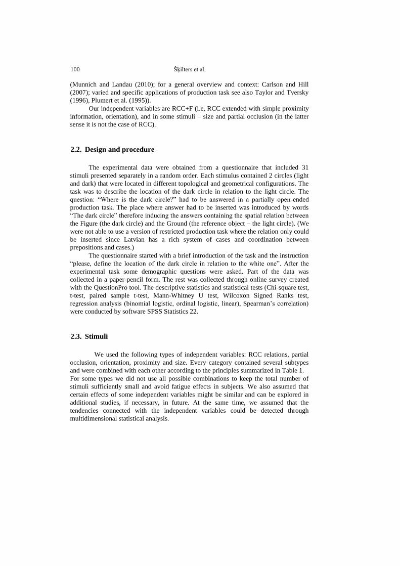
The experimental data were obtained from a questionnaire that included 31
stimuli presented separately in a random order. Each stimulus contained 2 circles (light
and dark) that were located in different topological and geometrical configurations. The
task was to describe the location of the dark circle in relation to the light circle. The
question: “Where is the dark circle?” had to be answered in a partially open-ended
production task. The place where answer had to be inserted was introduced by words
“The dark circle” therefore inducing the answers containing the spatial relation between
the Figure (the dark circle) and the Ground (the reference object – the light circle). (We
were not able to use a version of restricted production task where the relation only could
be inserted since Latvian has a rich system of cases and coordination between
prepositions and cases.)
The questionnaire started with a brief introduction of the task and the instruction
“please, define the location of the dark circle in relation to the white one”. After the
experimental task some demographic questions were asked. Part of the data was
collected in a paper-pencil form. The rest was collected through online survey created
with the QuestionPro tool. The descriptive statistics and statistical tests (Chi-square test,
t-test, paired sample t-test, Mann-Whitney U test, Wilcoxon Signed Ranks test,
regression analysis (binomial logistic, ordinal logistic, linear), Spearman’s correlation)
were conducted by software SPSS Statistics 22.
2.3. Stimuli
We used the following types of independent variables: RCC relations, partial
occlusion, orientation, proximity and size. Every category contained several subtypes
and were combined with each other according to the principles summarized in Table 1.
For some types we did not use all possible combinations to keep the total number of
stimuli sufficiently small and avoid fatigue effects in subjects. We also assumed that
certain effects of some independent variables might be similar and can be explored in
additional studies, if necessary, in future. At the same time, we assumed that the
tendencies connected with the independent variables could be detected through
multidimensional statistical analysis.
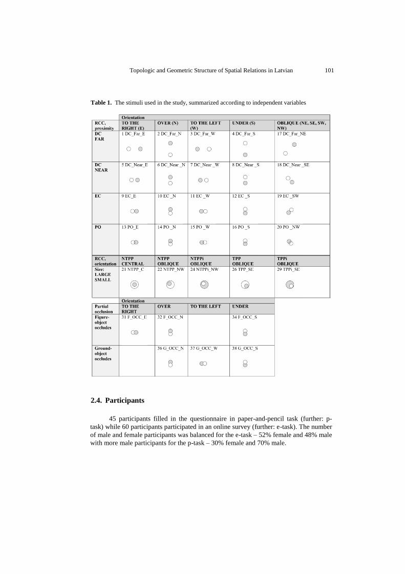
Topologic and Geometric Structure of Spatial Relations in Latvian 101
Table 1. The stimuli used in the study, summarized according to independent variables
2.4. Participants
45 participants filled in the questionnaire in paper-and-pencil task (further: p-
task) while 60 participants participated in an online survey (further: e-task). The number
of male and female participants was balanced for the e-task – 52% female and 48% male
with more male participants for the p-task – 30% female and 70% male.
102 Šķilters et al.
Almost all participants were native speakers of Latvian (in both tasks 3
participants indicated Russian as their native language) with English as the second
(91%) and Russian as the third (72%) best known language.
Most of the participants who filled in the e-task had university education (75%),
while 37% of the participants in p-task were with university education and 11% with
secondary school education. Humanities/social sciences were the most frequent fields of
education (60%) with the e-task participants. Most of the participants in the p-task were
from the fields of exact sciences; humanities and social sciences were represented by
34% participants. Also, we had to take into account the number of participants with
secondary school education who filled in the paper task, because they could not provide
information about field of education.
The age distribution of participants was similar in both tasks (p-task/e-task) –
younger than 25: 41%/30%; 25–34: 23%/27%; 35–44: 16%/23%; 45–54: 9%/8% and
older than 55: 11%/12%).
Demographic part also included questions regarding occupation and hobbies and
the place where they had lived for the most part of their lives. The electronic task ended
with the question about right-/left-handedness (92%/8%). Median time for completing
the electronic task was ~14 minutes.
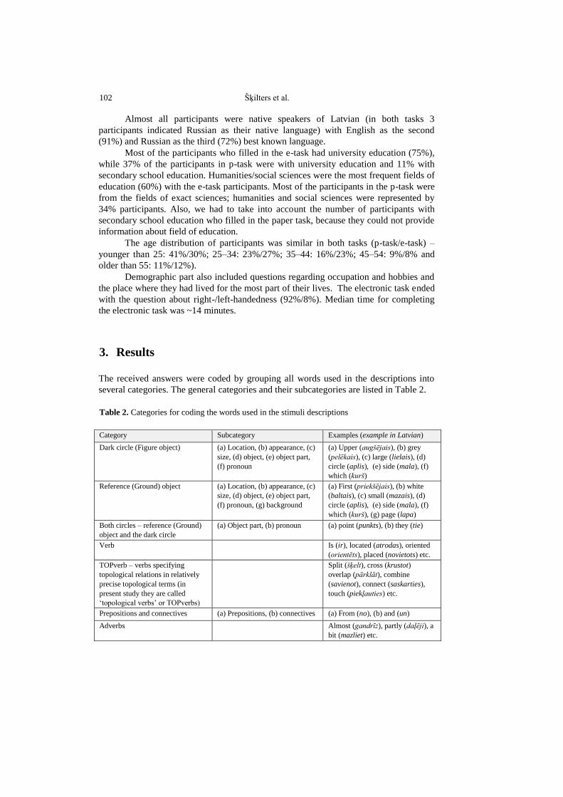
3. Results The received answers were coded by grouping all words used in the descriptions into
several categories. The general categories and their subcategories are listed in Table 2.
Table 2. Categories for coding the words used in the stimuli descriptions
Category Subcategory Examples (example in Latvian)
Dark circle (Figure object) (a) Location, (b) appearance, (c)
size, (d) object, (e) object part,
(f) pronoun
(a) Upper (augšējais), (b) grey (pelēkais), (c) large (lielais), (d)
circle (aplis), (e) side (mala), (f)
which (kurš) Reference (Ground) object (a) Location, (b) appearance, (c)
size, (d) object, (e) object part,
(f) pronoun, (g) background
(a) First (priekšējais), (b) white (baltais), (c) small (mazais), (d)
circle (aplis), (e) side (mala), (f)
which (kurš), (g) page (lapa)
Both circles – reference (Ground)
object and the dark circle (a) Object part, (b) pronoun (a) point (punkts), (b) they (tie)
Verb Is (ir), located (atrodas), oriented
(orientēts), placed (novietots) etc. TOPverb – verbs specifying
topological relations in relatively
precise topological terms (in
present study they are called
‘topological verbs’ or TOPverbs)
Split (šķelt), cross (krustot)
overlap (pārklāt), combine
(savienot), connect (saskarties),
touch (piekļauties) etc.
Prepositions and connectives (a) Prepositions, (b) connectives (a) From (no), (b) and (un)
Adverbs Almost (gandrīz), partly (daļēji), a
bit (mazliet) etc.

Topologic and Geometric Structure of Spatial Relations in Latvian 103
Direction (a) Cardinal directions, (b)
geometric directions (a) North (ziemeļi), (b) horizontal (horizontāli)
Distance (a) Relative distance, (b) size of
distance (a) Closer (tuvāk), (b)small (mazs)
Numbers ¼, 4, 30, at 19 o’clock (plkst.. 19)
etc. Measurements (a) Units of measurements, (b)
object as measure, (c) geometric
measures, (d) what is measured
(a) Percentages (procenti), (b)
piece (gabals), (c) angle (leņķis),
(d) distance (attālums) Localization prepositions Left, right, over, above, up, on,
under, below, down, behind,
inside, next to, in front of, in the
middle, in the center, between,
around
E.g., inside, in (iekšā, iekš,
iekšpusē, iekšīenē, ietvaros etc.)
Misc. Traffic-light (luksofors), target (mērķis), olympic ring
(olimpiskais aplis) etc.
We also introduced several additional variables listed in Table 3 below.
Table 3. Additionally introduced categories for coding the words used in stimuli descriptions
Additional variables Examples (example in Latvian)
Comparison form Smaller (mazākais), lower
(zemāk) Locative_Object In the circle (aplī)
Locative_ Localization words in locative In the middle (vidū)
Generalization of object part Side (mala), part (daļa), half
(puse), corner (stūris)
Word count of the description – amount of words used for the
description To the right (Pa labi) – 2 Next to the light circle (Blakus
gaišajam aplim) – 3
Accuracy of the description of the Figure’s location – measure was
determined according to the granularity of the information provided
to describe where the Figure is situated. (The detailed criteria are
given in: Zilinskaite et al., 2019)
To the right (Pa labi) – 1 To the right, next to the light
circle (Pa labi, blakus gaišajam
aplim) – 2
The categories, localization preposition subcategories (Table 2) and additional
variables (Table 3) were analysed as the dependent variables according to their
frequency and variety corresponding to each configuration (Table 1). The summary of
relative frequencies is summarized in Table 4 and Table 6. (frequencies below 5% are
not included.) Each relative frequency (%) reflects the amount of answers where words
belonging to the particular category had been used. Frequencies differ within each
category if the stimuli are compared. By the Chi-square test the differences over all
stimuli set in each coded category were tested and the significant ones (α=0.05) are
marked by blue and red colours.

104 Šķilters et al.
Table 4.1 Frequencies of the words used in the stimuli (Table 1) descriptions according the coded
categories (Table 2 and Table 3), %
Right (E) Left (W) Over (N)
1 D
C_
Far
_E
5 D
C_
Nea
r_E
9 E
C_E
13 P
O_
E
31 F
_O
CC
_E
3 D
C_
Far
_W
7 D
C_
Nea
r_W
11 E
C_
W
15 P
O_
W
37 G
_O
CC
_W
2 D
C_
Far
_N
6 D
C_
Nea
r_N
10 E
C_
N
14 P
O_
N
32 F
_O
CC
_N
36 G
_O
CC
_N
a)
Dark (Figure) circle
10 10 12 14 10 11 12 11 14 20 18 20 20 23 19 26
Reference
(Ground) object 50 51 54 60 61 49 51 54 62 66 61 60 62 70 69 67
Both circles
(common parts) 3 2 11 6 3 1 1 13 8 3 3 3 14 9 2 5
b)
Verbs 23 30 24 28 23 30 30 23 25 34 31 32 27 32 26 28
TOPverbs 4 7 27 35 29 3 4 27 37 17 5 6 28 40 30 23
c)
Prepos_Connect 50 47 32 38 29 43 46 35 35 22 21 22 15 34 23 25
Adverbs 9 11 17 25 23 11 10 16 20 20 10 10 17 24 20 23
d)
Direction 11 7 4 4 6 5 7 6 6 4 10 7 7 3 5 4
Distance_Size 9 10 0 5 2 7 7 0 2 3 9 12 2 4 4 5
Numbers 14 9 3 4 5 11 6 3 3 3 13 10 2 5 3 5
Measures 12 14 1 3 4 16 10 0 3 4 19 14 1 4 4 2
e)
Comparisons 5 2 1 2 2 3 3 2 2 2 3 8 4 5 2 4
Half 11 12 14 14 15 13 13 10 13 12 8 6 5 10 13 10
Side 0 0 7 4 3 0 0 5 3 5 0 2 5 2 4 3
Part 0 0 0 1 3 1 0 0 2 4 0 2 1 5 4 3
Corner
Blue – significantly less likely use of certain category according to Chi-Square test
Red – significantly more likely use of certain category according to Chi-Square test

Topologic and Geometric Structure of Spatial Relations in Latvian 105
Table 4.2. Frequencies of the words used in the stimuli (Table 1) descriptions according the
coded categories (Table 2 and Table 3), %
Under (S) Oblique In / Around
4 D
C_
Far
_S
8 D
C_
Nea
r_S
12 E
C_
S
16 P
O_
S
34 F
_O
CC
_S
38 G
_O
CC
_S
17 D
C_
Far
_N
E
18
DC
_N
ear_
SE
19 E
C_
SW
20 P
O_
NW
21 N
TP
P_C
22 N
TP
P_
NW
26 T
PP
_S
E
24 N
TP
Pi_
NW
29 T
PP
i_S
E
a)
Dark (Figure) circle
14 14 19 17 16 25 13 12 12 17 14 20 18 31 32
Reference
(Ground) object 61 55 63 70 67 66 59 59 58 65 70 73 74 70 63
Both circles
(common parts) 2 2 10 7 3 3 2 1 15 7 4 4 3 3 10
b)
Verbs 31 31 29 28 27 28 30 35 30 31 36 40 34 39 33
TOPverbs 4 6 20 34 28 20 1 5 27 38 4 6 14 17 19
c)
Prepos_Connect 23 23 11 35 29 23 53 55 45 40 19 24 27 16 18
Adverbs 12 10 17 16 26 23 10 11 12 18 4 5 6 11 6
d)
Direction 10 8 4 4 4 2 30 28 28 20 0 9 10 4 7
Distance_Size 13 10 2 8 9 5 12 10 6 5 8 7 3 4 8
Numbers 13 6 2 5 8 5 14 12 9 7 6 6 6 7 8
Measures 21 15 0 5 4 4 15 14 8 8 4 6 6 5 5
e)
Comparisons 9 7 7 9 6 4 10 7 8 5 13 15 15 17 20
Half 2 3 5 6 5 6 13 9 11 13 7 19 22 2 3
Side 0 0 5 2 4 4 0 1 3 3 0 4 7 2 4
Part 0 1 0 5 8 3 0 0 1 3 1 5 5 3 4
Corner 55 5
Blue – significantly less likely use of certain category according to Chi-Square test
Red – significantly more likely use of certain category according to Chi-Square test
The differences between stimuli in each coded category were explored using
binary logistic regression modelling employing the following factors: topological
relation, proximity, orientation and axial direction (Table 5). Similar results were
obtained by applying Chi-square test to separate groups of stimuli distinguished by these
factors. For example, all stimuli with EC relation were mutually compared with respect
to frequencies in coded categories, thus enabling to assess the impact of different

106 Šķilters et al.
orientations, or all stimuli where the dark circle is above the light one were mutually
compared with respect to frequencies in coded categories, thus enabling to assess the
impact of topological relations.
Table 5. Factors for exploring frequency differences within coded categories
1. Topological relations 2. Proximity/
distance 3. Orientation 4. Axial
direction DC – disconnectedness none to the left (W) horizontal
EC – externally connectedness near to the right (E) vertical
PO – partial overlap far
over (N) oblique
TPP – tangential proper part under (S) center
NTPP – non-tangential proper
part oblique, left-over
(SW)
TPPi – inverse tangential
proper part oblique, right-over
(SE)
NTPPi – inverse non-tangential
proper part oblique, right-under
(NE)
Figure-object occludes
(F_OCC) oblique, left-under
(NW)
Ground-object occludes
(G_OCC) center
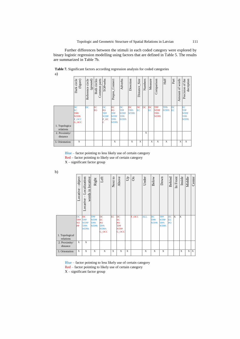
Further the impacts of the factors included in Table 5 and detected as statistically
significant (p=0.05) by Chi-square tests are described. The tendencies concluded from
regression analysis are summarized in Table 7a.
The dark circle (Table 4a) is significantly more frequently mentioned for stimuli
if it is around the white circle (NPPi, NTPPi) or behind it (Ground-object occludes)
while it is less frequently mentioned where both circles are not connected (DC),
especially if located to the right.
Similarly, the reference (Ground) object (Table 4a) is referred to differently
depending on connectedness. When circles are not connected (DC) the reference object
is mentioned less frequently, except for stimuli where the dark circle is in or around the
light circle (NTPP, NTPPi). For description of tangential and non-tangential proper part
stimuli (NTPP, TPP) the reference object is mentioned most frequently.
Common parts (e.g., shared areas of both circles, common point) (Table 4a) are
mentioned less frequently –5-15% answers in total for some stimuli. They are more
typical for those cases where circles are externally connected (EC) or overlapping (PO).
The use of verbs (Table 4b) does not differ significantly if different stimuli are
compared, but the use of TOPverbs (i.e., topological verbs) (Table 4b) differs
significantly depending on the topological relation. The main differences in the use of
TOPverbs refer to stimuli with overlapping circles (PO) (in these cases, TOPverbs are
used most frequently) and stimuli where both circles are not connected (DC) (in this
case, TOPverbs are used less frequently). The proximity (distance) does not show any

Topologic and Geometric Structure of Spatial Relations in Latvian 107
significant impact on the use of TOPverbs. Also, the general orientational information –
horizontal, vertical, oblique and central – shows no significant impact on the use of
TOPverbs. When looking in more in detail at the impact of orientation (to the left, to the
right, above, under, etc.) – the different frequencies regarding the use of TOPverbs are
due to connectedness of the circles.
The prepositions and connectives (Table 4c) are used to a lesser extent for
description of stimuli where the dark circle is in the center or around the light circle
(NTPP, NTPP) and has partial occlusion with respect to the light circle. Significantly
more frequent prepositions and connectives are used for stimuli where circles are not
connected (DC) and are located on the horizontal or oblique axis. Regarding the vertical
orientation, prepositions and connectives are more frequently used for those stimuli
where circles overlap, but less frequently when circles are not connected (DC) or are the
cases of objects touching (EC). However, we have to take into account that this category
is somewhat subtle and includes different words regarding their function in the
description (localization prepositional construction (e.g., to the left (pa kreisi)), sentence
construction (e.g., above and touching (augšpusē un pieskaras)) etc. Thus, the
differences may be linked with coding specifics, as we did not develop subcategories
according to different contexts. Similarly, the adverb category (Table 4c) includes
different words with respect to their context in the description and we are not
particularly interpreting the differences. Adverbs most frequently had been used in cases
when circles overlap or occludes. In turn, they are less frequently used in more
unambiguous situations when the dark circle is inside or around the light circle.
In stimuli where both objects are disconnected, significantly more frequently
specifying information is provided as to relational orientation, distance and further
measuring (including numerical information) items. The words in stimuli descriptions
that correspond to direction category (Table 4d) most frequently are used for the stimuli
that refer to the relations where circles are displayed on oblique axis (20-30%).
However, such tendency is not observed for stimuli with containment (TPP, NTPP,
TPPi, NTPPi) where circles are also on the oblique axis. The distance and size
information (Table 4d) is mentioned relatively more frequently for those stimuli where
circles do not touch (DC) (7-13%). The same refers to information that characterizes
measurements (10-21%) and includes numerical values (6-14%) (Table 4d).
Regarding comparison category (Table 4e), most frequently comparison forms
are used for containment stimuli (TPP, NTPP, TPPi, NTPPi). For locational
generalizations (Table 4e) such as ‘side’, ‘half’ and ‘edge’ most commonly the word
‘half’ is used and most often it is used for stimuli where the circles are either on the
horizontal or oblique axis except for the stimuli where the dark circle is around the light
one (TPPi, NTPPi) with the circles on the oblique axis, but overall it is not common to
use locational generalizations. In turn, when the dark circle is inside the light one on the
oblique axis (TPP, NTTP) use of generalization “half’ is significantly more frequent.
In particular, we explored the subcategories that refer to spatial information – the
localization prepositions (Table 2) and use of the locative (Table 3). The summary of
relative frequencies is provided in Table 6. With the Chi-square test the differences over
all stimuli set in each coded category were tested and the significant ones (α=0.05) are
marked in blue and red.

108 Šķilters et al.
Table 6.1. Frequencies of the words used in the stimuli (Table 1) descriptions according to the
coded categories (Table 2 and Table 3), %
Right (E) Left (W) Over (N)
1 D
C_
Far
_E
5 D
C_
Nea
r_E
9 E
C_E
13
PO
_E
31
F_
OC
C_
E
3 D
C_
Far
_W
7 D
C_
Nea
r_W
11
EC
_W
15
PO
_W
37
G_
OC
C_
W
2 D
C_
Far
_N
6 D
C_
Nea
r_N
10
EC
_N
14
PO
_N
32
F_
OC
C_
N
36
G_
OC
C_
N
a)aa)
Locative_object 0 4 6 8 6 1 5 6 8 6 0 2 4 7 5 4 Locative_location 22 6 6 6 5 24 6 4 4 9 42 17 12 9 7 4 b)
Right (Labā puse) 86 83 74 70 70 2 1 2 4 4 0 0 0 0 0 0 Left (Kreisā puse) 1 1 3 6 5 85 86 74 69 56 0 0 0 0 0 0 NextTo (Blakus) 10 10 32 9 6 12 9 32 7 7 3 8 8 2 2 2 Above (Virs) 0 0 0 2 23 0 0 2 1 1 48 50 51 35 55 23 Up (Augšā) 0 0 0 1 1 0 0 0 0 0 43 39 33 37 39 35 On (Uz) 0 0 0 0 2 0 1 0 0 1 1 0 3 0 5 0 Under (Zem) 0 0 0 12 0 0 0 1 12 27 0 0 0 11 0 22 Below (Apakšā) 0 0 0 1 0 0 0 0 0 2 1 0 1 2 2 4 Down (Lejā) 0 0 0 0 0 0 0 0 1 1 0 0 0 0 0 0 InFront (Priekšā) 1 2 1 3 12 2 2 0 1 0 0 0 0 3 11 0 Behind (Aiz) 0 1 0 10 0 0 0 0 11 28 1 1 1 11 0 29 Inside (Iekšā) 0 0 0 1 0 0 0 0 0 0 0 0 0 1 0 0 Middle (Vidū) 1 0 1 0 0 1 1 0 1 1 1 1 0 2 1 1 Centre (Centrā) 0 0 1 1 0 0 0 1 0 0 1 0 0 0 0 1 Around (Ap) 0 1 1 0 0 1 0 0 0 0 0 0 0 1 0 0
Blue – significantly less likely use of certain category according to Chi-Square test
Red – significantly more likely use of certain category expected according to Chi-Square test
Again, the general tendencies from the Table 6 were tested with Chi Square test
within stimuli groups distinguished according to the previously mentioned factors
(Table 5). Further the significant (p=0.05) tendencies have been described.
The locative with respect to a spatial object (Table 6a) is most frequently used for
containment stimuli where the dark circle is inside the light one (TPP, NTPP). For
containment stimuli with the dark circle around the light one (TPPi, NTPPi) the locative
form is also used but to a lesser extent. Also, the oblique axis is a factor supporting the
frequency of locative use.
Regarding the use of the location words in the locative (Table 6a) the determining
factors are connectedness – more use in such location forms when circles are not
connected (DC), and distance – mostly used when circles are far from each other (except

Topologic and Geometric Structure of Spatial Relations in Latvian 109
in the case when the dark circle is under the light one where this distance tendency is
opposite).
Table 6.2. Frequencies of the words used in the stimuli (Table 1) descriptions according to the
coded categories (Table 2 and Table 3), %
Under (S) Oblique In / Around
4 D
C_
Far
_S
8 D
C_
Nea
r_S
12 E
C_
S
16 P
O_
S
34 F
_O
CC
_S
38 G
_O
CC
_S
17 D
C_
Far
_N
E
18 D
C_
Nea
r_S
E
19 E
C_
SW
20 P
O_
NW
21 N
TP
P_C
22 N
TP
P_
NW
26 T
PP
_S
E
24 N
TP
Pi_
NW
29 T
PP
i_S
E
a)
Locative_object 0 1 4 6 4 3 9 9 9 11 31 34 43 12 16 Locative_location 18 21 7 5 7 7 12 9 7 9 4 2 0 1 2 b)
Right (Labā puse) 0 0 0 0 0 0 58 53 1 3 0 1 30 6 6 Left (Kreisā puse) 0 0 0 0 0 0 0 2 53 50 1 22 2 4 7 NextTo (Blakus) 4 4 6 2 2 0 3 10 16 2 0 0 3 0 1 Above (Virs) 1 0 0 6 25 1 13 0 1 13 6 8 9 3 1 Up (Augšā) 0 0 1 2 3 5 54 0 0 44 1 21 0 7 5 On (Uz) 0 0 0 2 4 0 0 0 0 0 7 10 9 1 0 Under (Zem) 49 45 55 41 25 52 0 19 13 15 0 2 0 26 25 Below (Apakšā) 19 22 25 30 21 27 0 10 17 2 0 0 10 0 4 Down (Lejā) 13 17 12 14 19 17 0 37 33 0 0 0 11 4 4 InFront (Priekšā) 1 1 1 2 18 0 1 1 1 2 7 7 8 0 0 Behind (Aiz) 0 0 0 9 0 20 1 0 0 10 0 0 0 26 25 Inside (Iekšā) 0 0 0 0 0 0 0 0 0 2 22 38 42 2 3 Middle (Vidū) 2 2 1 3 3 1 0 2 1 0 27 4 2 3 5 Centre (Centrā) 1 0 0 0 0 0 0 0 1 0 22 2 0 4 6 Around (Ap) 0 0 0 0 0 0 0 0 0 1 0 0 0 22 16
Blue – significantly less likely use of certain category according to Chi-Square test
Red – significantly more likely use of certain category expected according to Chi-Square test
Again, the general tendencies from the Table 6 were tested with Chi Square test
within stimuli groups distinguished according to the previously mentioned factors
(Table 5). Further the significant (p=0.05) tendencies have been described.
The locative with respect to a spatial object (Table 6a) is most frequently used for
containment stimuli where the dark circle is inside the light one (TPP, NTPP). For
containment stimuli with the dark circle around the light one (TPPi, NTPPi) the locative
form is also used but to a lesser extent. Also, the oblique axis is a factor supporting the
frequency of locative use.
Regarding the use of the location words in the locative (Table 6a) the
determining factors are connectedness – more use in such location forms when circles

110 Šķilters et al.
are not connected (DC), and distance – mostly used when circles are far from each other
(except in the case when the dark circle is under the light one where this distance
tendency is opposite).
Obviously, the left and the right orientation (Table 6b) are used for stimuli where
the dark circle is on the horizontal axis. Most commonly it is used is for stimuli where
the circles are not connected (DC), but the distance does not show significant impact.
Similarly, these location words are less but still commonly used for stimuli with the
oblique axis (50-58 %). Comparatively less they are used for containment stimuli with
the dark circle inside the light one (22-30%) (TPP, NTTP). For the stimuli with the dark
circle around the light one (TPPi, NTPPi) these location words are used rarely and most
likely for the description of location of the light circle with respect to the dark one even
if the task had been to use it as reference for the light circle.
Interesting is the use of the location ‘next to’(Table 6b). Most commonly it is
used for topological relation where circles are externally connected (EC) (most
pronounced effect on the horizontal axis), but there is tendency to use it also for the
relation when circles are not connected (DC) but lie on the horizontal axis.
The most common location words used for the ‘over’ (North direction) (Table
6b) are Up and Above. These words are commonly used also for the stimuli where the
dark circle is in front of the light circle (stimuli 31, 32, and 34, Table 1) indicating the
3D perspective. Also, the containment stimuli descriptions indicate that 3D perspective
has been used, e.g., for stimuli 21 and 26 (Table 1). For the oblique axis, a more typical
way of interpreting the ‘above’ it is to use the word Up.
The most common location words used for the ‘under’ (South direction) (Table
6b) are Under, Below and Down. The location word Under seems to be characteristic
for 3D perspective, as it is used for the stimuli where circles overlap or the dark circle is
behind the light one, as well as in the case when the dark circle is around the light one
(TPPi, NTPPi). The Under and Below locations are used also for the oblique axis
stimuli, however Down is more frequently used for these situations. Below and Down
are also among the descriptions of stimuli where the dark circle is inside the light one
externally connected at a point in oblique direction (stimuli 24, Table1).
In front location is used for descriptions of stimuli where the dark circle is in
front of the light circle (Figure-object occludes, stimuli 31, 32, and 34) (Table 6b). We
can also observe 3D perspective for those stimuli where the dark circle is inside the light
circle (TPP, NTPP, stimuli 21, 22, 26), but the frequencies are relatively small (7-8%).
More pronounced this perspective is in case when the dark circle is around the light one
(TPPi, NTPPi, stimuli 24, 29), and Behind is used for description in around 25% cases.
Use of Behind reflects also in the stimuli where circles overlap (PO, Stimuli 13-16) –
around 10% cases. For the stimuli where the dark circle is behind the light one (Ground-
object occludes, stimuli 36, 37, 38) the use of Behind varies from 20-29%.
For the description of proper part stimuli where the dark circle is inside the light
one (TPP, NTPP) the commonly used location is Inside and in case of central location
of the dark circle (stimuli 21) – also Middle and Center. In the situation when the dark
circle is around the light one (TPPi, NTPPi) the commonly used location is Around, but
just 16-22%, demonstrating that 2D perspective is less common if compared to the
situation when the dark circle is Figure rather than Background.
Topologic and Geometric Structure of Spatial Relations in Latvian 111
Further differences between the stimuli in each coded category were explored by
binary logistic regression modelling using factors that are defined in Table 5. The results
are summarized in Table 7b.
Table 7. Significant factors according regression analysis for coded categories
a)
Dar
k c
ircl
e
(fig
ure
)
Ref
eren
ce c
ircl
e
(gro
und
)
Both
cir
cles
Co
mm
on
par
ts
TO
Pv
erb
s
Pre
pos_
Conn
ect
Ad
ver
bs
Dir
ecti
on
Dis
tan
ce_
Siz
e
Nu
mber
s
Mea
sure
Co
mp
aris
on
Hal
f
Par
t
Am
oun
t o
f w
ord
s
Pre
cisi
on
of
the
dec
ripti
on
1. Topologica
relations
DC
EC
TPPi
NTPPi
F_OCC
G_OCC
DC EC
PO
DC
PO
TPP
NTPP
F_OC
C
DC
PO
TPP
NTPP
TPPi
NTPPi
DC
TPP
NTPP
TPPi
NTPPi
DC
TPPi
NTPPi
DC
EC
DC
DC
EC
TPP
NTPP
TPPi
NTPPi
TPPi
NTPPi
DC
EC
EC
TPP
NTPP
TPPi
NTPPi
2. Proximity/
distance
X
3. Orientation X X X X X X X X
X
Blue – factor pointing to less likely use of certain category
Red – factor pointing to likely use of certain category
X – significant factor group
b)
Lo
cati
ve
- o
bje
ct
Lo
cari
ve
– L
oca
liza
tion
wo
rds
in l
oca
tiv
e
Rig
ht
Lef
t
Nex
t to
Ab
ov
e
Up
On
Un
der
Bel
ow
Do
wn
Beh
ind
In F
ron
t
Insi
de
Mid
dle
Cen
ter
1. Topological
relations
DC
TPP
NT
PP
DC
TPP
NTPP
TPPi
NTPPi
TPP
NTPP
TPPi
NTPPi
DC
EC
PO
TPPi
NTPPi
G_OCC
EC DC
EC
PO
TPP
NTPP
G_OCC
F_OCC ALL DC
TPPi
NTPPi
TPP
NTPP
TPPi
NTPPi
DC
EC
PO
X X
2. Proximity/
distance
X X
3. Orientation X X X X X X X X X X X X
X
Blue – factor pointing to less likely use of certain category
Red – factor pointing to likely use of certain category
X – significant factor group

112 Šķilters et al.
Different stimuli were described by different number of words and also the
accuracy of the localization (Table 3) was given at different level. The length of
descriptions seems to correlate with the degree of specificity that is needed to
communicate the relation unambiguously. According to our results, we can observe that
the more words are used the more accurately the location of the dark circle is given
(Spearman’s rho = 0.786, significance level = 0.01). Therefore, the systematic
differences between relations in terms of the length of their descriptions indicate that not
all relations are equally specific and require more descriptive details.
There was no significant difference (t-test (words), Mann-Whitney U test
(localization) for each stimuli, α=0.05) between these indicators depending on whether
the answers were obtained in a paper pencil test or in online survey (except, for the
stimulus ‘5 Close_Right’ the localization description precision was statistically different
(Mean_e-task=1.77, Mean_ptask=1.36). Accordingly, further analysis was conducted
taking into account these differences, but when possible – the electronic and paper
answers were analyzed together as equal.
By paired sample t-test (words) and Wilcoxon Signed-Rank test (localization) we
tested the differences depending on stimuli and were able to formulate several
homogenous subgroups regarding the number of words and localization precision
(Figure 1, Figure 2).
Figure 1. Average number of words used for each subset of stimuli description
with significantly different subgroups of stimuli.
Data show that fewest words are used for the stimuli that describe vertical
direction in simple topological relations (not connected (DC, far and close) and
connected at one point (EC)) as well as inside the central area (Stimuli 21). Most words
are used for the same simple relations (DC, EC) when the direction is oblique. Most
words in average are used for the situation of overlapping in oblique direction which
might indicate that this relation is descriptively most complex. Also, other overlapping
situations are described with more words than the same directions for other topological
relations (not connected (DC), connected (EC), partial occlusion with respect to the light
circle (behind (G_OCC), in front (F_OCC))). We conducted linear regression analysis
using the factors listed in Table 5. The obtained model pointed to orientation as a
significant factor (Table 7a).
Topologic and Geometric Structure of Spatial Relations in Latvian 113
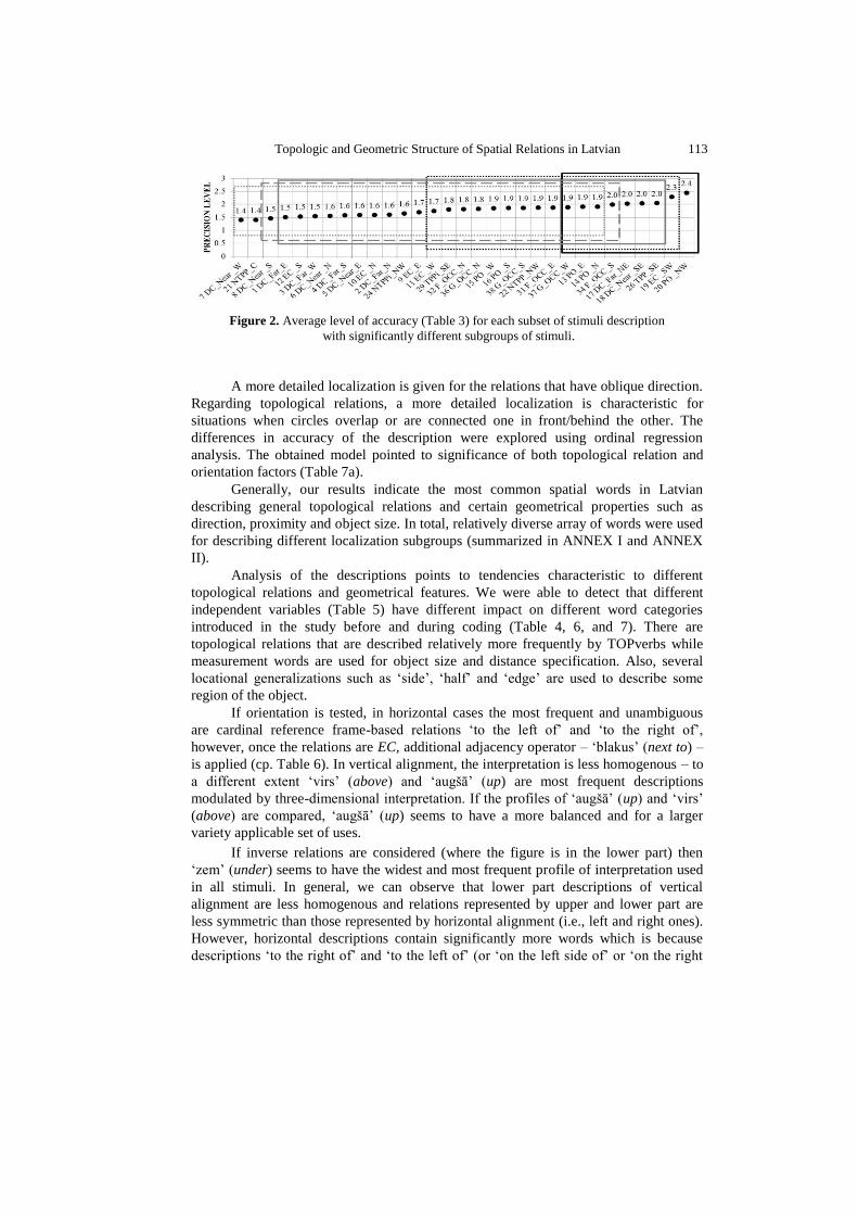
Figure 2. Average level of accuracy (Table 3) for each subset of stimuli description
with significantly different subgroups of stimuli.
A more detailed localization is given for the relations that have oblique direction.
Regarding topological relations, a more detailed localization is characteristic for
situations when circles overlap or are connected one in front/behind the other. The
differences in accuracy of the description were explored using ordinal regression
analysis. The obtained model pointed to significance of both topological relation and
orientation factors (Table 7a).
Generally, our results indicate the most common spatial words in Latvian
describing general topological relations and certain geometrical properties such as
direction, proximity and object size. In total, relatively diverse array of words were used
for describing different localization subgroups (summarized in ANNEX I and ANNEX
II).
Analysis of the descriptions points to tendencies characteristic to different
topological relations and geometrical features. We were able to detect that different
independent variables (Table 5) have different impact on different word categories
introduced in the study before and during coding (Table 4, 6, and 7). There are
topological relations that are described relatively more frequently by TOPverbs while
measurement words are used for object size and distance specification. Also, several
locational generalizations such as ‘side’, ‘half’ and ‘edge’ are used to describe some
region of the object.
If orientation is tested, in horizontal cases the most frequent and unambiguous
are cardinal reference frame-based relations ‘to the left of’ and ‘to the right of’,
however, once the relations are EC, additional adjacency operator – ‘blakus’ (next to) –
is applied (cp. Table 6). In vertical alignment, the interpretation is less homogenous – to
a different extent ‘virs’ (above) and ‘augšā’ (up) are most frequent descriptions
modulated by three-dimensional interpretation. If the profiles of ‘augšā’ (up) and ‘virs’
(above) are compared, ‘augšā’ (up) seems to have a more balanced and for a larger
variety applicable set of uses.
If inverse relations are considered (where the figure is in the lower part) then
‘zem’ (under) seems to have the widest and most frequent profile of interpretation used
in all stimuli. In general, we can observe that lower part descriptions of vertical
alignment are less homogenous and relations represented by upper and lower part are
less symmetric than those represented by horizontal alignment (i.e., left and right ones).
However, horizontal descriptions contain significantly more words which is because
descriptions ‘to the right of’ and ‘to the left of’ (or ‘on the left side of’ or ‘on the right

114 Šķilters et al.
side of_’) consist of several words each. Partly this might also indicate that relations
based on the vertical alignment are less ambiguous (Figure 1).
Generally, topological relations are significant factors for every category. A
significant feature of the perception of PO is three-dimensionality. Stimuli 31 and 37
(and inversely – 15 and 37) are perceived three-dimensionally but the three-dimensional
interpretation is more dominating in the case where the figure object partially overlaps
without transparency effects than in case if the overlapping figure is transparent. I.e., the
transparent cases (13 and 15) are interpreted less three-dimensionally than not
transparent ones (31 and 37). This might eventually be because of the perceptual effects
of amodal completion. These descriptions contain ‘virs’ (above) 25%, ‘priekšā’ (in front
of) 12 % and ‘zem’ (under) 27% , ‘aiz’ (behind) 28% (see Table 6). Somewhat similar
pattern of results arises in vertical interpretation. Cases of non-transparent overlapping
(stimuli 32, 34, 36, and 38) allow three-dimensional interpretation of ‘aiz’ (behind) and
‘priekšā’ (in front of) again eventually in virtue of amodal completion.
In total, there is a variety of answers in our results sharing the principle that the
figure and ground object are bound by a spatial relation R(𝐹, 𝐺).
In most cases, they can be put in an ordered sequence ⟨𝐹, 𝑅, 𝐺⟩: 𝑅 ∈ RCC+F,
where the complete version would be either
[The black square]𝐹𝑖𝑔𝑢𝑟𝑒 [is]𝑉𝑒𝑟𝑏[in front of]𝑃𝑃[the white circle]𝐺𝑟𝑜𝑢𝑛𝑑
or
[The black square]𝐹𝑖𝑔𝑢𝑟𝑒 [is put]𝑉𝑒𝑟𝑏[on the top of]𝑃𝑃[the white circle]𝐺𝑟𝑜𝑢𝑛𝑑.
According to Landau et al. (Johannes et al., 2016a, b, Landau et al., 2017), the
latter case contains a lexical verb which contributes to the meaning of expression,
whereas the former case contains a copular verb which in turn does not significantly
contribute to the overall meaning of the expression. According to Landau’s framework,
lexical verbs are more force-dynamic than geometric. Further, gravitational support as
the core relation of support (also when compared cross-linguistically and
developmentally, cp. Landau et al. (2017). According to our results that we explore in a
more detail elsewhere (Žilinskaite-Šinkūniene et al., 2019), in functionally simple
stimuli also (such as RCC+F) we can observe different and complex impacts of support
and containment on the interpretation of spatial relations and their representation in
natural language.
4. Discussion A general observation is that the horizontally aligned configuration induces a more
symmetric, whereas vertical – less symmetric interpretation. Eventually this is because
of support relation operating in vertical alignment. According to previous research
((Maki et al., 1977), for discussion: (Newcombe and Huttenlocher, 2000, 185f.)),
horizontal and vertical axial structures seem to be difficult and salient to a different
degree; horizontal axial information (left / right) is more difficult than vertical (above /
below) and vertical axis seems to be more salient which is also reflected why ‘south/
north’ is recognized easier than ‘east/ west’ (Loftus, 1978). As to the difference in the
strength of axial structures, (a) the vertical axis is gravity determined and therefore the

Topologic and Geometric Structure of Spatial Relations in Latvian 115
strongest, whereas (b) front-back is weaker, and the most difficult is (c) the left-right
axial structure (Newcombe and Huttenlocher, 2000).
Notwithstanding the differences mentioned before, our results seem to support
the view that vertical and horizontal alignments are cognitively more prominent with
respect to other relations (cp. (Hayward and Tarr, 1995)).
According to several recent studies by Barbara Landau and her colleagues (cp.
(Johannes et al., 2016b) which used natural scenes, basic locative expressions and
expressions of support seem to represent a part of the core of spatial knowledge that is
relatively robust in developmental terms. Further, gravitational support is most
prominent if natural scenes are observed; in our simplified stimuli we cannot see the
detailed structure support or containment (as in the case of everyday objects), some
functional constraints might eventually apply, e.g., if vertical and horizontal alignments
are compared (for a more detailed discussion of support and containment in Baltic
languages cp. (Žilinskaite-Šinkūniene et al., 2019)).
Proximity as a factor seems to be important but to a different degree in different
cases. It seems to impact the use of ‘blakus’ (next to).
According to our results, relational descriptions are preferred over metric or
continuous ones (which tends to support findings by Lovett and Franconeri (2017), cp.
also Yuan et al. (2016)). Relational descriptions that enable segmenting space into rather
discrete categories are preferred with a relative consistency. Further, relatively precise
topological expressions (using TOPverbs) are applied. We might also agree that
categorical relations between objects seem to be more stable than changes in size
(Lovett and Franconeri, 2017).
However, the fact that observers segment spatial relations categorically does not
mean that the categories are mutually exclusive; rather categories overlap and fuzzy
category borders seem to be the case in most situations (Newcombe and Huttenlocher,
2000, 183). There are spatial descriptors that are more universal (or prototypic) for
certain relations (e.g., ‘virs’ (above)) and some that are more specific (‘uz’(on)).
Eventually, we might hypothesize that the most prototypical descriptions are used to
understand the less prototypic ones (Newcombe and Huttenlocher, 2000, 184).
According to our results, topological relations (e.g., EC vs. DC) seem to be
relatively primary with respect to geometric ones; however, this is a tentative statement
since the object form, distance and angular information seem to have a more complex
determining role too and will be explored in an upcoming paper. The primacy of
topological descriptions also supports findings by Knauff et al. (1997). According to
their results, most of the descriptions of RCC relations are topological and there is only
a small number of combinations of topological and orientational (14,1%) and
topological and metric information (19,2%) (Knauff et al., 1997).
We also agree that topological relations are primary with respect to fine-grained
geometric relations and that processing of spatial information is most likely a stage-wise
process where objects (their topological boundaries) are discriminated in the first stage,
then primary relations are generated and more detailed geometric knowledge is added at
a later point (cp. also (Franconeri et al., 2012), (Xu and Franconeri, 2012), (Choo et al.,
2012), (Chen, 2005a, b)).
Consistent with the idea that primary processing stage is topologic, we agree with
Palmer and Rock (1994) about the principle of uniform connectedness stating that the
primary operation is generation of perceptual units that takes place in virtue of

116 Šķilters et al.
connectedness and is occurring at an entry level of perception and is therefore prior to
grouping. Although we assume that basic topological relations (complemented with
some geometric and functional primitives) allow optimal representation of spatial
relations, we were able to show that not all topological and geometric relations are
interpreted equally: e.g., some have a wider scope of interpretation and some –
narrower; some seem to induce a more precise description, whereas others – less (E.g.
‘under’ and ‘on’ can be interpreted in 2D and 3D perspectives, but ‘centre’ can be
interpreted unambiguously).
Our results indirectly support Roth and Franconeri (2012) findings about
asymmetric coding of spatial relations. E.g., ‘black circle is below the white circle’ is
interpreted differently than ‘white circle is below the black circle’. This is reflected in
the principle that an object that has to be located needs another object providing a
reference area where the former is located. Roth and Franconeri (2012) showed the
effect of this asymmetry by using the analysis of selective attention and arguing that
attention is mapped onto one object at a time; the figure object is marked by the
spotlight of attention. According to these results, asymmetry in spatial coding seems to
be shared by perceptual and linguistic levels. In our case this distinction can be nicely
seen in linguistic descriptions induced by
𝑄: Where is 𝐹?
and observing the answer
𝐴: 𝑅(𝐹, 𝐺)
which in virtue of the asymmetry can be expressed in an ordered triplet ⟨𝐹, 𝑅, 𝐺⟩, e.g.,
⟨Circle, in front of, square⟩, indicating that canonical interpretation binds figure and
ground object with a relation – prepositional or otherwise (for an application and
discussion of figure and ground relationship as a spatial extraction principle within geo-
referencing approach cp. (Chen et al., 2017.)).
In perceptual terms, our results eventually also support the findings by Lester et
al. (2009) that figural regions are available for perceptual processing before the grounds;
however, this seems to be the case only when figure and ground are not spatially
separated or at least share an edge.
We also argue that proximity impacts the perception of topological and
geometric relations but to a more complex degree in case of each relation. Although
spatial proximity seems to be a more crucial factor than others (Franconeri et al, 2012),
its impact is different in different configurations.
Our results seem to at least partially to support the view proposed by Chen
(2005a, b, 1982) that primary level of perceptual processing is topological both in terms
of object individuation and spatial relations: according to Chen topological relations and
topological organization based on physical connectedness are primary with respect to
geometric (based on distance). In our case, topological relations are more detailed than
geometric ones. However, distance plays a crucial role in some of the relations,
according to our results. Another explanation might be that a certain tolerance space
(Peters and Wasilewski, 2012) generation principle applies according to which some
elements (close to one another) are perceived as one or belonging to one another.
Connectedness as a core topological feature (Chen, 1982) seems to have impact
in the interpretation of spatial relations which is also consistent with our results (cp.
Table 7 reflects the significance for several categories).

Topologic and Geometric Structure of Spatial Relations in Latvian 117
Once we have geometrical primitive of nearness, the formal level of our
approach is compatible with tolerance and nearness models ((Peters, 2007), (Peters and
Wasilewski, 2009, 2012); for an analysis of proximity cp. also (Peters and Guadagni,
2016)).
In fact, the idea of tolerance qualities is close to the principle of proximity by
Claude Vandeloise: “A point acquires the quality of another point as long as it is not
closer to a third point bearing the contradictory quality.” (1991, 48) Although the
principle of proximity according to Vandeloise applies to functional relations and
contexts, it makes perfect sense to be used for topological settings as well.
Finally, our work supports the results and generalizations by Klippel et al.
(2013). According to our findings not all topological relations are equally prominent
and some geometric factors (such as orientation and distance) matter as well. Although
we did not test different semantic domains (as done in the studies by Klippel) we made a
more careful analysis of RCC-based spatial relations that are relatively neutral in terms
of semantic domain and therefore our results can serve as a precise foundational basis
for exploring other domains. To sum up, according to our results, we would like to
argue that topology is not sufficient to generate a cognitively valid model of spatial
representation – some geometrical and functional primitives are also needed. Although
we have not tested other than static stimuli, we agree that dynamic stimuli and stimuli
reflecting the manner of motion shape the perception of the ‘underlying’ topology.
Finally, we assume that topology and geometry, and functional factors have different
temporal properties – it might be the case that topology matters at the temporarily
primary level but is context-dependently modulated by geometric and functional
constraints at a slightly later point.
Our work shows cognitive relevance and plausibility of an RCC-based model.
Although spatial representations are always to some extent language-dependent, natural
languages never exactly encode metric relations (instead relational representations are
used) (cp. (Newcombe and Huttenlocher, 2000)) enabling RCC to be a cognitively
plausible and sensitive way of expressing relational representations of spatial language.
5. Conclusions
According to our results, (1) proximity seems to be a sensitive independent
variable - when using a larger distance between F and G in several spatial relations a
larger percentage of consistent descriptions are generated by users whereas if the
distance is smaller the variety of other descriptions is increasing. However, proximity
and distance impact only some relations (cp. Table 7). (2) In all spatial relations (but to
a different degree in each) a set of topological verbs is used that relatively precisely
describe the spatial relations (Table 4). (3) in most RCC+F relations spatial relations are
encoded and linguistically represented categorically instead of encoding fine-grained
details. (4) It seems that the most robust topological relations can be grouped into (a)
those where there are no shared points between both objects (basically all varieties of
DC) and (b) contained objects (TPP and NTPP). (5) Topological and geometric (e.g.,
axial alignment, distance) relations matter but to a different degree. (6) In case of
different relations, different descriptive accuracy can be achieved. Finally, (7) we have

118 Šķilters et al.
tested both paper-and-pencil and digital versions and were not able to see significant
differences in the description accuracy of RCC+F relations between both formats.
However, we have left for further studies the analysis of the use of different location
prepositions for the same configuration or differences between word use depending on
the test version (p-task vs e-task). Therefore, we might assume that there are subtler
differences between both formats.
Our study extends the understanding of how topological relations are encoded in
natural language (e.g., topological verbs show a relatively precise set of descriptive
tools worth to be explored in future studies). Our results can also be used in natural
language systems when more precise descriptive tools are necessary for representing
spatial relations.
Acknowledgements
This research has been supported by the European Regional Development Fund within
the project “Neural Network Modelling for Inflected Natural Languages” No.
1.1.1.1/16/A/215.
References Amir, O., Biederman, I., Herald, S. B., Shah, M. P., Mintz, T. H. (2014). Greater sensitivity to
nonaccidental than metric shape properties in preschool children. Vision Research, 97,
83–88.
Aurnague, M., Vieu, L. (1993). Toward a formal representation of space in language: A
commonsense reasoning approach. In IJCAI-93 workshop on spatial and temporal
reasoning (pp. 123-158).
Carlson, L. A., Hill, P. L. (2007). Experimental methods for studying language and space. In M.
Gonzalez-Marquez, I. Mittelberg, S. Coulson, M.J. Spivey (Eds.), Methods in Cognitive
Linguistics (pp. 250-276). Amsterdam: John Benjamins Publishing.
Chen, H., Vasardani, M., Winter, S. (2017). Geo-referencing Place from Everyday Natural
Language Descriptions. arXiv preprint arXiv:1710.03346. Chen, L. (1982). Topological
structure in visual perception. Science, 218(4573), 699-700.
Chen, L. (2005a). The topological approach to perceptual organization. Visual Cognition, 12(4),
553-637.
Chen, L. (2005b). Author’s response: Where to begin? Visual Cognition, 12(4), 691-701.
Choo, H., Franconeri, S. L. (2010). Visual size averaging of objects unavailable to conscious
awareness. Attention, Perception, & Psychophysics, 72(1), 86-99.
Choo, H., Levinthal, B. R., Franconeri, S. L. (2012). Average orientation is more accessible
through object boundaries than surface features. Journal of Experimental Psychology:
Human Perception and Performance, 38(3), 585-588.
Clementini, E., Di Felice, P., Van Oosterom, P. (1993). A small set of formal topological
relationships suitable for end-user interaction. In D. Abel, B.C. Ooi (Eds.), Advances in
spatial databases. Third International Symposium on Spatial Databases (pp. 277-295).
Berlin: Springer.
Cohn, A. G., Bennett, B., Gooday, J., Gotts, N. M. (1997). Qualitative spatial representation and
reasoning with the region connection calculus. GeoInformatica, 1(3), 275-316.

Topologic and Geometric Structure of Spatial Relations in Latvian 119
Coventry, K. R., Garrod, S. C. (2004). Saying, seeing and acting: The psychological semantics of
spatial prepositions. Hove: Psychology Press.
Coventry, K. R., Prat-Sala, M., Richards, L. (2001). The interplay between geometry and function
in the comprehension of over, under, above, and below. Journal of memory and language,
44(3), 376-398.
Davis, E., Marcus, G., Frazier-Logue, N. (2017). Commonsense reasoning about containers using
radically incomplete information. Artificial Intelligence, 248, 46-84.
Della Penna, G., Magazzeni, D., Orefice, S. (2017). A formal framework to represent spatial
knowledge. Knowledge and Information Systems, 51(1), 311-338.
Düntsch, I., Wang, H., McCloskey, S. (2001). A relation-algebraic approach to the region
connection calculus. Theoretical Computer Science, 255(1), 63-83.
Egenhofer, M. J., Franzosa, R. D. (1991). Point-set topological spatial relations. International
Journal of Geographical Information System, 5(2), 161-174.
Forbus, K. D., Chang, M., McLure, M., Usher, M. (2017). The cognitive science of sketch
worksheets. Topics in cognitive science, 9(4), 921-942.
Forbus, K.D. (2018). Qualitative representations: how people reason and learn about the
continuous world. Cambridge, MA: The MIT Press.
Franconeri, S. L., Pylyshyn, Z. W., Scholl, B. J. (2012). A simple proximity heuristic allows
tracking of multiple objects through occlusion. Attention, Perception, & Psychophysics,
74(4), 691-702.
Franconeri, S. L., Scimeca, J. M., Roth, J. C., Helseth, S. A., Kahn, L. E. (2012). Flexible visual
processing of spatial relationships. Cognition, 122(2), 210-227.
Gentner, D., Imai, M., Boroditsky, L. (2002). As time goes by: Evidence for two systems in
processing space→ time metaphors. Language and cognitive processes, 17(5), 537-565.
Gerevini, A., Renz, J. (2002). Combining topological and size information for spatial reasoning.
Artificial Intelligence, 137(1-2), 1-42.
Haun, D. B., Rapold, C. J., Janzen, G., Levinson, S. C. (2011). Plasticity of human spatial
cognition: Spatial language and cognition covary across cultures. Cognition, 119(1), 70-
80.
Hayes, P.J. (1985). The second naïve physics manifesto. In J. Hobbs, B. Moore (Eds.), Formal
theories of the commonsense world (pp. 1-36). Norwood, NJ: Ablex Publishing
Corporation.
Hayward, W. G., Tarr, M. J. (1995). Spatial language and spatial representation. Cognition, 55(1),
39-84.
Holmes, K. J., Moty, K., Regier, T. (2017). Revisiting the role of language in spatial cognition:
Categorical perception of spatial relations in English and Korean speakers. Psychonomic
bulletin & review, 24(6), 2031-2036.
Jamrozik, A., Gentner, D. (2015). Well-hidden regularities: Abstract uses of in and on retain an
aspect of their spatial meaning. Cognitive Science, 39.1881-1911.
Johannes, K., Wilson, C., Landau, B. (2016a). Systematic feature variation underlies adults’ and
children’s use of in and on. In Proceedings of the 38th Annual Meeting of the Cognitive
Science Society (pp. 2429-2434).
Johannes, K., Wilson, C., Landau, B. (2016b). The importance of lexical verbs in the acquisition
of spatial prepositions: The case of in and on. Cognition, 157, 174-189.
Klippel, A., Li, R., Yang, J., Hardisty, F., Xu, S. (2013). The Egenhofer–Cohn Hypothesis or,
Topological Relativity? In M. Raubal et al. (Eds.), Cognitive and linguistic aspects of
geographic space (pp. 195-215). Springer, Berlin, Heidelberg.
Kluth T, Burigo M, Schultheis H, Knoeferle P (2017) In: Proceedings of the 10th Embodied and
Situated Language Processing Conference, Moscow, Russia. Moscow, Russia: 26-27.
120 Šķilters et al.
Knauff M., Rauh R., Renz J. (1997) A cognitive assessment of topological spatial relations:
Results from an empirical investigation. In S.C. Hirtle, A.U. Frank (Eds.). Spatial
Information Theory: A Theoretical Basis for GIS. COSIT 1997. Lecture Notes in
Computer Science, vol 1329. (pp. 193-206). Springer: Berlin, Heidelberg.
https://doi.org/10.1007/3-540-63623-4_51
Knauff, M. (1999). The cognitive adequacy of Allen's interval calculus for qualitative spatial
representation and reasoning. Spatial Cognition and Computation, 1(3), 261-290.
Kosslyn, S. M., Murphy, G. L., Bemesderfer, M. E., Feinstein, K. J. (1977). Category and
continuum in mental comparisons. Journal of Experimental Psychology: General, 106,
341–375.
Kracht, M. (2002). On the semantics of locatives. Linguistics and Philosophy, 25(2), 157-232.
Maki, R. H., Maki, W. S., Marsh, L. G. (1977). Processing locational and orientational
information. Memory & Cognition, 5(5), 602-612.
Kranjec, A., Cardillo, E. R., Schmidt, G. L., Chatterjee, A. (2010). Prescribed spatial prepositions
influence how we think about time. Cognition, 114(1), 111-116.
Landau, B. (2017). Update on “what” and “where” in spatial language: a new division of labor for
spatial terms. Cognitive science, 41(S2), 321-350.
Landau, B. (2017). Update on “what” and “where” in spatial language: a new division of labor for
spatial terms. Cognitive science, 41(S2), 321-350.
Lester, B. D., Hecht, L. N., Vecera, S. P. (2009). Visual prior entry for foreground figures.
Psychonomic Bulletin & Review, 16(4), 654-659.
Loftus, G. R. (1978). Comprehending compass directions. Memory & Cognition, 6(4), 416-422.
Logan, G.D., Sadler, D.D. (1996). A computational analysis of the apprehension of spatial
relations. In P. Bloom, M.A. Peterson, L. Nadel, M.F. Garrett (Eds.). Language and space
(pp. 493-529). Cambridge, MA: MIT Press.
Lovett, A., Franconeri, S. L. (2017). Topological relations between objects are categorically
coded. Psychological science, 28(10), 1408-1418.
Mantle, M., Batsakis, S., Antoniou, G. (2019). Large scale distributed spatio-temporal reasoning
using real-world knowledge graphs. Knowledge-Based Systems, 163, 214-226.
Mani, I., Pustejovsky, J. (2012). Interpreting motion: Grounded representations for spatial
language. Oxford: Oxford University Press.
Munnich, E., Landau, B. (2010). Developmental decline in the acquisition of spatial language.
Language Learning and Development, 6(1), 32-59.
Newcombe, N. S., Huttenlocher, J. (2000). Making space: The development of spatial
representation and reasoning. Cambridge, MA: The MIT Press.
Palmer, S., Rock, I. (1994). Rethinking perceptual organization: The role of uniform
connectedness. Psychonomic bulletin & review, 1(1), 29-55.
Peters, J. F. (2007). Near sets. General theory about nearness of objects. Applied Mathematical
Sciences, 1(53), 2609-2029.
Peters, J. F., Guadagni, C. (2016). Strongly proximal continuity & strong connectedness.
Topology and its Applications, 204, 41-50.
Peters, J. F., Wasilewski, P. (2009). Foundations of near sets. Information Sciences, 179(18),
3091-3109.
Peters, J. F., Wasilewski, P. (2012). Tolerance spaces: Origins, theoretical aspects and
applications. Information Sciences, 195, 211-225.
Plumert, J. M., Carswell, C., Devet, K., Ihrig, D. (1995). The content and organization of
communication about object locations. Journal of Memory and Language, 34(4), 477498.
Pustejovsky, J., Lee, K. (2017). Enriching the Notion of Path in ISO-Space. In Proceedings of the 13th Joint ISO-ACL Workshop on Interoperable Semantic Annotation (ISA-13).
Randell, D. A., Cui, Z., Cohn, A. G. (1992). A spatial logic based on regions and connection. KR,
92, 165-176.

Topologic and Geometric Structure of Spatial Relations in Latvian 121
Rodrigues, E., Santos, P. E., Lopes, M. (2017). Pinning down polysemy: A formalisation for a
Brazilian Portuguese preposition. Cognitive Systems Research, 41, 84-92.
Roth, J., Franconeri, S. (2012). Asymmetric coding of categorical spatial relations in both
language and vision. Frontiers in psychology, 3, 464.
Skilters, J., Zarina, L., Glanzberg, M., Zilinskaite, E. (in prep.) RCC+F: some applications in
Baltic languages.
Shen, J., Chen, M., Yue, S. (2018). A distance-based topological relation model between spatial
regions. Arabian Journal of Geosciences, 11(23), 763.
Stell, J. G. (2000). Boolean connection algebras: a new approach to the Region-Connection
Calculus. Artificial Intelligence, 122(1-2), 111-136.
Svenonius, P. (2006) The emergence of axial parts. Nordlyd: Tromsø Working Papers in
Linguistics, 33.1, 49-77.
Talmy, L. (1975). Figure and ground in complex sentences. In Annual Meeting of the Berkeley
Linguistics Society, Vol. 1, pp. 419-430.
Taylor, H. A., Tversky, B. (1996). Perspective in spatial descriptions. Journal of memory and
language, 35(3), 371-391.
Vandeloise, C. (1991). Spatial prepositions: A case study from French. Chicago: The University
of Chicago Press.
Vasardani, M., Stirling, L. F., Winter, S. (2017). The preposition at from a spatial language,
cognition, and information systems perspective. Semantics and Pragmatics, 10.
Vieu, L. (1997). Spatial representation and reasoning in artificial intelligence. In O. Stock (Ed.).
Spatial and temporal reasoning (pp. 5-41). Dordrecht: Springer.
Xu, Y., Franconeri, S. L. (2012). The head of the table: Marking the “front” of an object is tightly
linked with selection. Journal of neuroscience, 32(4), 1408-1412.
Yuan, L., Uttal, D., Franconeri, S. (2016). Are categorical spatial relations encoded by shifting
visual attention between objects? PloS one, 11(10), e0163141.
Zilinskaite-Sinkuniene, E., Šķilters, J., Zariņa, L. (2019). Containment and support in Baltic
languages: Overview, experimental evidence, and an extended RCC as applied to Latvian
and Lithuanian. Baltic Journal of Modern Computing, Vol. 7 (2019), No. 2, 224–254.
https://doi.org/10.22364/bjmc.2019.7.2.02
Zwarts, J. (1997). Vectors as Relative Positions: A Compositional Semantics of Modified PPs1.
Journal of semantics, 14(1), 57-86.
Zwarts, J., Winter, Y. (2000). Vector space semantics: A model-theoretic analysis of locative
prepositions. Journal of logic, language and information, 9(2), 169-211.
Received September 22, 2019, revised February 13, 2020, accepted March 7, 2020

122 Šķilters et al.
Annexes
ANNEX I
Most common spatial words in Latvian language - localization subgroups
Pa labi (Right
side) Zem
(Under) Virs
(Above) Aiz (Behind) Iekšā (Inside) Ap (Around)
pa labi zem virs aiz iekšā ap labajā/labā ZEM_ virsū aizmugurē iekš apkārt LAB_ Zem
(Below) virspuse fonā iekšpuse ārējā
Pa kreisi (Left
side) apakšā pa virsu pēc iekšiene ārpusē pa kreisi apakšējā VIRS_ ēnā ietvaros ārā kreisajā/kreisā apakšpusē Augšā
(Up) AIZ_ IEKŠ_ ĀR_
KREIS_ apakšmala augšā Priekšā (In
Front) Vidū (Middle) Starp
(Between) Blakus (Next
To) pamatā augšup priekšā vidū starp
blakus saknē augšējā priekšplāns pa vidu Pār (Over) atstatus apakš uz augšu pretī vidusdaļa pār netālu APAKŠ_ no augšas pirms viducī
pie Lejā
(Down) augšpuse priekšpusē no vidus
līdzās lejā galvenē pirmajā plānā Centrā
(Central) nostatus uz leju augšdaļa
centrā sānis lejpus augšmalā ne centrā klāt lejum augsti iecentrēts gar leja AUGS/Š_ nav iecentrēts kopā lejasdaļā Uz (On) koncentrisks nostāk
uz ekscentriski ķēdē
centrēti
pa centru

Topologic and Geometric Structure of Spatial Relations in Latvian 123
ANNEX II
Words used in stimuli descriptions grouped by coded categories
Darbības
vārdi
(Verb)
Topoloģiski darbības v.
(TOPverbs) Prievārdi
(Prepositions)
Apstākļa vārdi
(Adverbs)
ir / esošs nav kopīgu
punktu atdalījies no aptuveni gandrīz
atrodas nesaskaras iebrauc ar krietni ne aiziet saskaras ieritinājies pa kādu vienlaicīgi nobīdīts šķērso nepieskarties par daļēji apmēram novirzīts krusto apēdis uz nedaudz viegli atdevis pārsedz ieskaut pret tieši tā novietots pārklāj saplūst pēc cieši ļoti sēž aptver apņem Saikļi
(Connectives) uzreiz absolūti
tiek ietver sastopas un daudz drīzāk nebūt šķeļ sakrīt vai gluži pašā iekrāsot saķerē nesavienoties jeb mazliet
neatrasties savienots apsegt arī pilnībā iet kombinācijā nepārklāties bet samērā atstāt aizsedz sakļauties kā kopīgs saglabāt pieskaras mīties kas ap ievietot savijies segt nekā savstarpējs vērsts aizklāj caurvijas nu relatīvi dotie nosedz ietilpst ka attiecībā atbilst aizskar nepiekļauties gan ievērojami orientēts piekļaujas kontaktā tomēr vairāk stāvēt aizslēpts
brīvi veido iekļaut
attālināties paslēpts

124 Šķilters et al.
Virziens (Direction) Attālums
(Distance) Mēri (Measures)
Debesu puses
(Cardinal)
Attālums
relatīvi
(Relative
distance) Skaitļi (Numbers)
Mērvienības
(Units of
measurements)
Ko mēra
(What is
measured)
A augstāk 1/5 60 reizes attālums R tālāk 1/4 70 grādi atstarpe Z tuvāk 1/3 90 procenti distance D citur 1/2 135 km stāvokis ZA zemāk 2/3 225 cm novietojums DA netālu 3/4 315 mm nobīde
DR pus viens Plkst.14.00
Objekts
(Object as
measure) teritorija ZR attālāk neviens Plkst. 3 aplis atrašanās
vieta Ģeometriski
(Geometric) nākamais 1, 5 Plkst. 4:30 gabals augstums
vertikāli viszemāk divi Plkst.4-5 krustojums pozīcija diagonāli turpat abi Plkst.6 pārklājums stāvs virzienā šeit 2,5 Plkst. 7:30 aizsegums
prom
Attāluma
izmērs (Size of
distance) 4 Plkst.10
Ģeometriski
(Geometric)
horizontāli liels 5 Plkst.17.00 diametrs slīpi neliels 10 Plkst.19 radiuss sānis paliels 11 vairāki leņķis taisni mazs 12 -π/4 ass paralēli vidējs 20 - 3π/4 korpuss v=(0,-2d/3) vienāds 30
garums šķērsām augošs 45 lielums y ass tas pats
pulkstens x projekcija citāds
tajā pašā līmenī dažāds
tāds
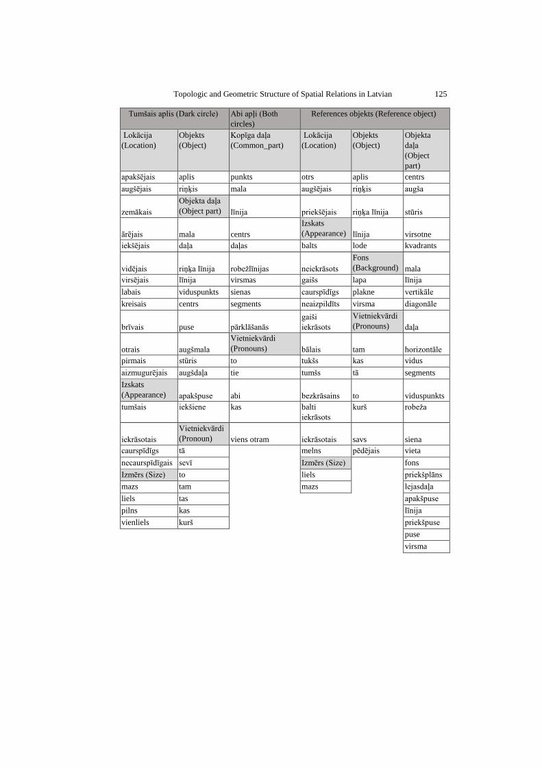
Topologic and Geometric Structure of Spatial Relations in Latvian 125
Tumšais aplis (Dark circle) Abi apļi (Both
circles)
References objekts (Reference object)
Lokācija
(Location)
Objekts
(Object)
Kopīga daļa
(Common_part)
Lokācija
(Location)
Objekts
(Object)
Objekta
daļa
(Object
part)
apakšējais aplis punkts otrs aplis centrs
augšējais riņķis mala augšējais riņķis augša
zemākais
Objekta daļa
(Object part) līnija priekšējais riņķa līnija stūris
ārējais mala centrs
Izskats
(Appearance) līnija virsotne
iekšējais daļa daļas balts lode kvadrants
vidējais riņķa līnija robežlīnijas neiekrāsots
Fons
(Background) mala
virsējais līnija virsmas gaišs lapa līnija
labais viduspunkts sienas caurspīdīgs plakne vertikāle
kreisais centrs segments neaizpildīts virsma diagonāle
brīvais puse pārklāšanās
gaiši
iekrāsots
Vietniekvārdi
(Pronouns) daļa
otrais augšmala
Vietniekvārdi
(Pronouns) bālais tam horizontāle
pirmais stūris to tukšs kas vidus
aizmugurējais augšdaļa tie tumšs tā segments
Izskats
(Appearance) apakšpuse abi bezkrāsains to viduspunkts
tumšais iekšiene kas balti
iekrāsots
kurš robeža
iekrāsotais
Vietniekvārdi
(Pronoun) viens otram iekrāsotais savs siena
caurspīdīgs tā
melns pēdējais vieta
necaurspīdīgais sevī Izmērs (Size)
fons
Izmērs (Size) to liels priekšplāns
mazs tam mazs lejasdaļa
liels tas
apakšpuse
pilns kas līnija
vienliels kurš priekšpuse
puse
virsma