Topics on Final Perceptrons SVMs Precision/Recall/ROC Decision Trees Naive Bayes Bayesian networks...
66
Topics on Final • Perceptrons • SVMs • Precision/Recall/ROC • Decision Trees • Naive Bayes • Bayesian networks • Adaboost • Genetic algorithms • Q learning • Not on the final: MLPs, PCA
-
Upload
bertina-pope -
Category
Documents
-
view
221 -
download
2
Transcript of Topics on Final Perceptrons SVMs Precision/Recall/ROC Decision Trees Naive Bayes Bayesian networks...

Topics on Final
• Perceptrons• SVMs• Precision/Recall/ROC• Decision Trees• Naive Bayes• Bayesian networks• Adaboost• Genetic algorithms• Q learning
• Not on the final: MLPs, PCA

Rules for Final
• Open book, notes, computer, calculator
• No discussion with others
• You can ask me or Dona general questions about a topic
• Read each question carefully
• Hand in your own work only
• Turn in to box at CS front desk or to me (hardcopy or e-mail) by 5pm Wednesday, March 21.
• No extensions

Short recap of important topics

Perceptrons

Training a perceptron
1. Start with random weights, w = (w1, w2, ... , wn).
2. Select training example (xk, tk).
3. Run the perceptron with input xk and weights w to obtain o.
4. Let be the learning rate (a user-set parameter). Now,
5. Go to 2.
€
wi ← wi + Δwi
where
Δwi = η (t k − ok )x ik

Support Vector Machines

• Here, assume positive and negative instances are to be separated by the hyperplane
€
w⋅x+b = 0
€
w⋅x+b = wT x + b
= w1x1 + w2x2 + b = 0
Equation of line:
x2
x1

• Intuition: the best hyperplane (for future generalization) will “maximally” separate the examples
€
w⋅ x + b = 0

Definition of Margin

Minimizing ||w||
Find w and b by doing the following minimization:
This is a quadratic optimization problem. Use “standard optimization tools” to solve it.
€
minw,b
1
2w
2 ⎛
⎝ ⎜
⎞
⎠ ⎟
subject to :
y i w⋅ x i + b( ) ≥1, i =1,...,m
(y i ∈{−1,+1})

• Dual formulation: It turns out that w can be expressed as a linear combination of a small subset of the training examples xi: those that lie exactly on margin (minimum distance to hyperplane):
such that xi lie exactly on the margin.
• These training examples are called “support vectors”. They carry all relevant information about the classification problem.
€
w= α ii
∑ x i

• The results of the SVM training algorithm (involving solving a quadratic programming problem) are the i and the bias b.
• The support vectors are all xi such that i > 0.
• Clarification: In the slides below we use i to denote
|i| yi , where yi {−1, 1}.

• For a new example x, We can now classify x using the support vectors:
• This is the resulting SVM classifier.
€
class(x) = sgn α i x⋅ xii∈ training examples{ }
∑ + b) ⎛
⎝ ⎜ ⎜
⎞
⎠ ⎟ ⎟

SVM review
• Equation of line: w1x1 + w2x2 + b = 0
• Define margin using:
• Margin distance:
• To maximize the margin, we minimize ||w|| subject to the constraint that positive examplesfall on one side of the margin, and negativeexamples on the other side:
• We can relax this constraint using “slack variables”
€
x i⋅w + b ≥ +1 for positive instances (y i = +1)
x i⋅w + b ≤ −1 for negative instances (y i = −1)
€
1
w
€
y i w⋅ x i + b( ) ≥1, i =1,...,m
where y i ∈{−1,+1}

SVM review
• To do the optimization, we use the dual formulation:
The results of the optimization “black box” are and b .
The support vectors are all xi such that i != 0.
€
w = α ix ii∈{training examples}
∑
€
{α i}

SVM review
• Once the optimization is done, we can classify a newexample x as follows:
That is, classification is done entirely through a linearcombination of dot products with training examples. This is a “kernel” method.
€
h(x) = class(x) = sgn w⋅ x + b( )
= sgn α ix ii=1
m
∑ ⎛
⎝ ⎜
⎞
⎠ ⎟⋅ x + b
⎛
⎝ ⎜ ⎜
⎞
⎠ ⎟ ⎟
= sgn α i x i⋅ x( )i=1
m
∑ ⎛
⎝ ⎜
⎞
⎠ ⎟+ b
⎛
⎝ ⎜ ⎜
⎞
⎠ ⎟ ⎟

Example
1 2-1-2
1
2
-2
-1

Example
1 2-1-2
1
2
-2
-1
Input to SVM optimzer:
x1 x2 class1 1 11 2 12 1 1-1 0 -10 -1 -1-1 -1 -1

Example
1 2-1-2
1
2
-2
-1
Input to SVM optimzer:
x1 x2 class1 1 11 2 12 1 1-1 0 -10 -1 -1-1 -1 -1
Output from SVM optimzer:
Support vector α(-1, 0) -.208(1, 1) .416(0, -1) -.208
b = -.376

Example
1 2-1-2
1
2
-2
-1
Input to SVM optimzer:
x1 x2 class1 1 11 2 12 1 1-1 0 -10 -1 -1-1 -1 -1
Output from SVM optimzer:
Support vector α(-1, 0) -.208(1, 1) .416(0, -1) -.208
b = -.376
€
w = α ix ii∈{training examples}
∑
= −.208 (−1,0) + .416 (1,1) − .208 (0,−1)
= (.624,.624)
Weight vector:

Example
1 2-1-2
1
2
-2
-1
Input to SVM optimzer:
x1 x2 class1 1 11 2 12 1 1-1 0 -10 -1 -1-1 -1 -1
Output from SVM optimzer:
Support vector α(-1, 0) -.208(1, 1) .416(0, -1) -.208
b = -.376
€
w = α ix ii∈{training examples}
∑
= −.208 (−1,0) + .416 (1,1) − .208 (0,−1)
= (.624,.624)
Weight vector:
Separation line:
€
w1x1 + w2x2 + b = 0
.624x1 + .624x2 − .376 = 0
x2 = −x1 + .6

Example
1 2-1-2
1
2
-2
-1
Classifying a new point:
€
h((2,2)) = sgn α i x i⋅ x( )i=1
m
∑ ⎛
⎝ ⎜
⎞
⎠ ⎟+ b
⎛
⎝ ⎜ ⎜
⎞
⎠ ⎟ ⎟
= sgn −.208 (−1,0)⋅ (2,2)[ ] + .416 (1,1)⋅ (2,2)[ ] − .208 (0,−1)⋅ (2,2)[ ] − .376( )
= sgn .416 +1.664 + .416 − .376( ) = +1

Precision/Recall/ROC

€
P =TP
TP + FP
€
R =TP
TP + FN
Results of classifier
Threshold Accuracy Precision Recall
.9
.8
.7
.6
.5
.4
.3
.2
.1
-∞
Creating a Precision/Recall Curve
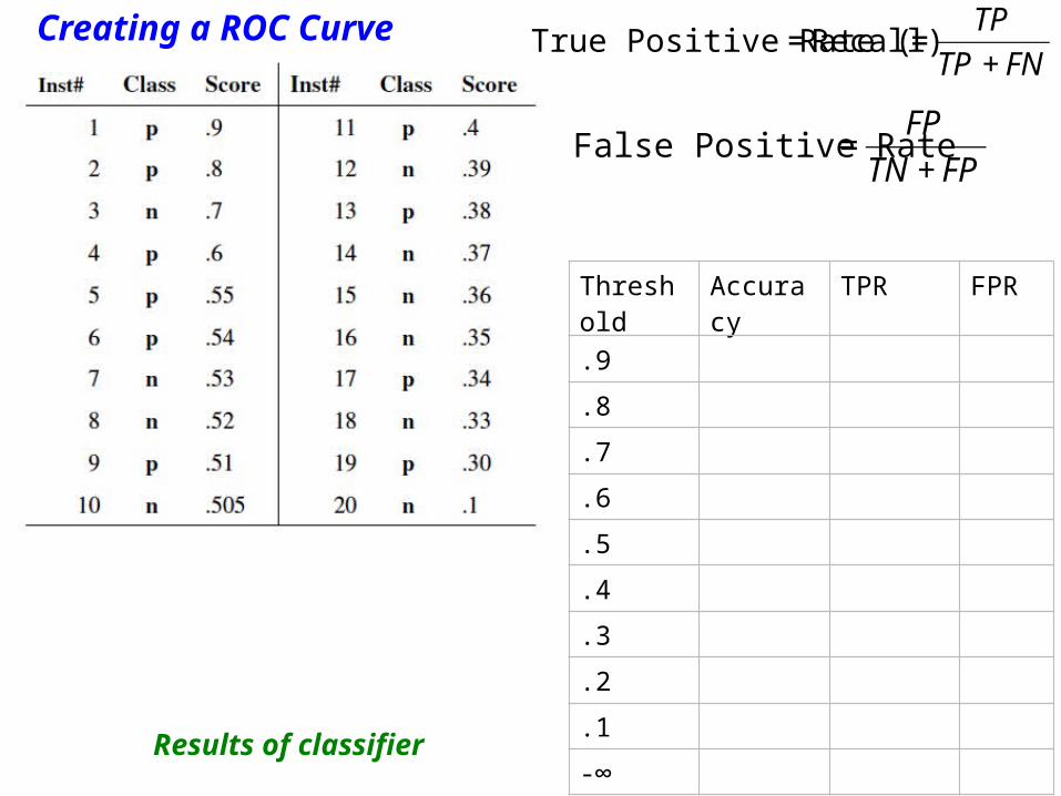
€
True Positive Rate (= Recall) =TP
TP + FN
€
False Positive Rate =FP
TN + FP
Results of classifier
Threshold Accuracy TPR FPR
.9
.8
.7
.6
.5
.4
.3
.2
.1
-∞
Creating a ROC Curve

26
Precision/Recall versus ROC curves
http://blog.crowdflower.com/2008/06/aggregate-turker-judgments-threshold-calibration/

27

Decision Trees

Naive Bayes

Naive Bayes classifier:
Assume
Given this assumption, here’s how to classify an instance
x = <a1, a2, ...,an>:
We can estimate the values of these various probabilities over the training set.
€
P(a1,a2,...,an | c j ) = P(a1 | c j )P(a2 | c j )L P(an | c j )
€
cNB (x) =c j ∈classesargmax P(c j ) P(ai
i
∏ | c j )
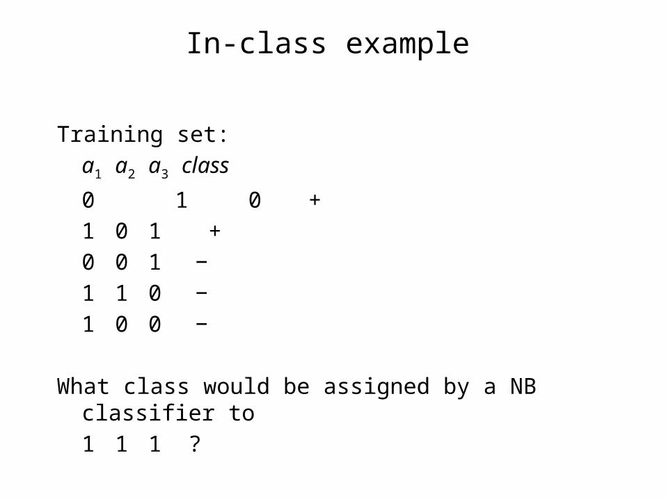
In-class example
Training set:
a1 a2 a3 class
0 1 0 +
1 0 1 +
0 0 1 −
1 1 0 −
1 0 0 −
What class would be assigned by a NB classifier to
1 1 1 ?

Laplace smoothing (also called “add-one” smoothing)
For each class cj and attribute ai with value z, add one “virtual” instance.
That is, recalculate:
where k is the number of possible values of attribute a.
a1 a2 a3 class Smoothed P(a1=1 | +) =
0 1 0 + Smoothed P(a1=0 | +) =
0 0 1 + Smoothed P(a1=1 | −) =
1 1 1 − Smoothed P(a1=0 | −) =
1 1 0 −
1 0 1 −
€
P(ai | c j ) ≈n(ai = z | c j ) +1
n(c j ) + k


Bayesian Networks

Methods used in computing probabilities
• Definition of conditional probability: P(A | B) = P (A,B) / P(B)
• Bayes theorem: P(A | B) = P(B | A) P(A) / P(B)
• Semantics of Bayesian networks:P(A ^ B ^ C ^ D)
= P(A | Parents(A)) P(B | Parents(B)) P(C | Parents(C)) P(D |Parents(D))
• Caculating marginal probabilities

What is P(Cloudy| Sprinkler)?
€
P(C | S) =P(S | C)P(C)
P(S)
=P(S | C)P(C)
P(S | C)P(C) + P(S | ¬ C)P(¬ C)
=(.1)(.5)
(.1)(.5) + (.5)(.5)
=(.05)
.3= .17

What is P(Cloudy| Wet Grass)?
€
P(C |W ) =P(C,W )
P(W )
=P(C,R,W ,S) + P(C,R,W ,¬ S) + P(C,¬ R,W ,S) + P(C,¬ R,W ,¬ S)
P(W )
=1
P(W )
P(C)P(R | C)P(W | R,S)P(S | C)
+P(C)P(R | C)P(W | R,¬ S)P(¬ S | C)
+P(C)P(¬ R | C)P(W | R,S)P(S | C)
+P(C)P(¬ R | C)P(W | ¬ R,¬ S)P(¬ S | C)
⎡
⎣
⎢ ⎢ ⎢ ⎢
⎤
⎦
⎥ ⎥ ⎥ ⎥

Markov Chain Monte Carlo Algorithm
• Markov blanket of a variable Xi:
– parents, children, children’s other parents
• MCMC algorithm:
For a given set of evidence variables {Xj=xk}
Repeat for NumSamples:– Start with random sample from variables, with evidence variables
fixed: (x1, ..., xn). This is the current “state” of the algorithm.
– Next state: Randomly sample value for one non-evidence variable Xi , conditioned on current values in “Markov Blanket” of Xi.
Finally, return the estimated distribution of each non-evidence variable Xi

Example
• Query: What is P(Sprinkler =true | WetGrass = true)?
• MCMC: – Random sample, with evidence variables fixed:
[Cloudy, Sprinkler, Rain, WetGrass]
= [true, true, false, true]
– Repeat:
1. Sample Cloudy, given current values of its Markov blanket: Sprinkler = true, Rain = false. Suppose result is false. New state: [false, true, false, true]
Note that current values of Markov blanket remain fixed.
2. Sample Sprinkler, given current values of its Markov blanket:
Cloudy = false, Rain= false, Wet = true. Suppose
result is true. New state: [false, true, false, true].

• Each sample contributes to estimate for query
P(Sprinkler = true| WetGrass = true)
• Suppose we perform 50 such samples, 20 with Sprinkler = true and 30 with Sprinkler= false.
• Then answer to the query is
Normalize (20,30) = .4,.6

Adaboost

Sketch of algorithm
Given data S and learning algorithm L:
• Repeatedly run L on training sets St S to produce h1, h2, ... , hT.
• At each step, derive St from S by choosing examples probabilistically according to probability distribution wt. Use St to learn ht.
• At each step, derive wt+1 by giving more probability to examples that were misclassified at step t.
• The final ensemble classifier H is a weighted sum of the ht’s, with each weight being a function of the corresponding ht’s error on its training set.

Adaboost algorithm
• Given S = {(x1, y1), ..., (xN, yN)} where x X, yi {+1, -1}
• Initialize w1(i) = 1/N. (Uniform distribution over data)

• For t = 1, ..., T:
– Select new training set St from S with replacement, according to wt
– Train L on St to obtain hypothesis ht
– Compute the training error t of ht on S :
– If t 0.5, break from loop.
– Compute coefficient
€
ε t = wti=1
N
∑ (i)I(y i ≠ ht (x i)) , where
I(y i ≠ ht (x i)) =1 if y i ≠ ht (x i)
0 otherwise
⎧ ⎨ ⎩
t
tt ε
εα 1ln
2
1

– Compute new weights on data:
where Zt is a normalization factor chosen so that wt+1 will be a probability distribution:€
wt +1(i) =wt (i) exp(−α t y iht (x i))
Zt
€
Zt =i=1
N
∑ wt (i) exp(−α t y iht (x i))

• At the end of T iterations of this algorithm, we have
h1, h2, . . . , hT
We also have
1, 2, . . . ,T, where
• Ensemble classifier:
• Note that hypotheses with higher accuracy on their training sets are
weighted more strongly.
)(sgn)(1
xx t
T
tthH
α
t
tt ε
εα 1ln
2
1

A Simple Example
t =1• S = Spam8.train:
x1, x2, x3, x4 (class +1)
x5, x6, x7, x8 (class -1)
• w1 = {1/8, 1/8, 1/8, 1/8, 1/8, 1/8, 1/8, 1/8}
• S1 = {x1, x2, x2, x5, x5, x6, x7, x8}
• Run svm_light on S1 to get h1
• Run h1 on S. Classifications: {1, -1, -1, -1, -1, -1, -1, -1}
• Calculate error:
€
ε1 = wti=1
N
∑ (i)I(y i ≠ ht (x i))
=1
83( ) = .375

• Calculate ’s:
• Calculate new w’s: €
α1 =1
2ln
1−ε t
ε t
⎛
⎝ ⎜
⎞
⎠ ⎟= .255
€
wt +1(i) =wt (i) exp(−α t y iht (x i))
Zt
ˆ w 2(1) = (.125)exp(−.255(1)(1)) = 0.1
ˆ w 2(2) = (.125)exp(−.255(1)(−1)) = 0.16
ˆ w 2(3) = (.125)exp(−.255(1)(−1)) = 0.16
ˆ w 2(4) = (.125)exp(−.255(1)(−1)) = 0.16
ˆ w 2(5) = (.125)exp(−.255(−1)(−1)) = 0.1
ˆ w 2(6) = (.125)exp(−.255(−1)(−1)) = 0.1
ˆ w 2(7) = (.125)exp(−.255(−1)(−1)) = 0.1
ˆ w 2(8) = (.125)exp(−.255(−1)(−1)) = 0.1
Z1 = ˆ w 2i
∑ (i) = .98
€
w2(1) = 0.1/.98 = 0.102
w2(2) = 0.163
w2(3) = 0.163
w2(4) = 0.163
w2(5) = 0.102
w2(6) = 0.102
w2(7) = 0.102
w2(8) = 0.102

t =2
• w2 = {0.102, 0.163, 0.163, 0.163, 0.102, 0.102, 0.102, 0.102}
• S2 = {x1, x2, x2, x3, x4, x4, x7, x8}
• Run svm_light on S2 to get h2
• Run h2 on S. Classifications: {1, 1, 1, 1, 1, 1, 1, 1}
• Calculate error:
€
ε 2 = wti=1
N
∑ (i)I(y i ≠ ht (x i))
= (.102) × 4 = 0.408

• Calculate ’s:
• Calculate w’s: €
α2 =1
2ln
1 −ε t
ε t
⎛
⎝ ⎜
⎞
⎠ ⎟= .186
€
wt +1(i) =wt (i) exp(−α t y iht (x i))
Zt
ˆ w 3(1) = (.102)exp(−.186(1)(1)) = 0.08
ˆ w 3(2) = (.163)exp(−.186(1)(1)) = 0.135
ˆ w 3(3) = (.163)exp(−.186(1)(1)) = 0.135
ˆ w 3(4) = (.163)exp(−.186(1)(1)) = 0.135
ˆ w 3(5) = (.102)exp(−.186(−1)(1)) = 0.122
ˆ w 3(6) = (.102)exp(−.186(−1)(1)) = 0.122
ˆ w 3(7) = (.102)exp(−.186(1)(1)) = 0.122
ˆ w 3(8) = (.102)exp(−.186(−1)(1)) = 0.122
Z2 = ˆ w 2i
∑ (i) = .973
€
w3(1) = 0.08 /.973 = 0.082
w3(2) = 0.139
ˆ w 3(3) = 0.139
ˆ w 3(4) = 0.139
ˆ w 3(5) = 0.125
ˆ w 3(6) = 0.125
ˆ w 3(7) = 0.125
ˆ w 3(8) = 0.125

t =3
• w3 = {0.082, 0.139, 0.139, 0.139, 0.125, 0.125, 0.125, 0.125}
• S3 = {x2, x3, x3, x3, x5, x6, x7, x8}
• Run svm_light on S3 to get h3
• Run h3 on S. Classifications: {1, 1, -1, 1, -1,- 1, 1, -1}
• Calculate error:
€
ε3 = wti=1
N
∑ (i)I(y i ≠ ht (x i))
= (.139) + (.125) = 0.264

• Calculate ’s:
• Ensemble classifier:
€
α3 =1
2ln
1 −ε t
ε t
⎛
⎝ ⎜
⎞
⎠ ⎟= .512
€
H(x) = sgn α tt =1
T
∑ ht (x)
= sgn .255 × S1(x) + .186 × S2(x) + .512 × S3(x)( )

• On test examples 1-8:
€
H(x) = sgn α tt =1
T
∑ ht (x)
= sgn .255 × S1(x) + .186 × S2(x) + .512 × S3(x)( )
S1 S2 S3
x1 1 1 1
x2 -1 1 -1
x3 -1 1 -1
x4 1 1 1
x5 -1 1 1
x6 -1 1 1
x7 -1 1 -1
x8 -1 1 1
Test accuracy: 3/8

Genetic Algorithms

Selection methods
• Fitness proportionate selection
• Rank selection
• Elite selection
• Tournament selection

Example
individual 1: 30
individual 2: 20
individual 3: 50
individual 4: 10
• Fitness proportionate probabilities?
• Rank probabilities?
• Elite probabilities (top 50%)?
Fitness

Reinforcement Learning / Q Learning

Q learning algorithm
– For each (s, a), initialize Q(s,a) to be zero (or small value).
– Observe the current state s.
– Do forever: • Select an action a and execute it. • Receive immediate reward r• Learn:
– Observe the new state s– Update the table entry for Q(s,a) as follows:
Q(s,a) Q(s,a) + η (r + γ maxa´ Q(s´,a´) – Q(s, a))
• s s

Simple illustrationof Q learning
C gives reward of 5 points.Each action has reward of -1.
No other rewards or penalties.
States are numbered squares
Actions (N, E, S, W) are selected at random.
Assume γ = 0.8, η = 1
R
C
1 2 3
4 5 6

Step 1Current state s = 1
R
C
1 2 3
4 5 6
Q(s,a) N S E W
1 0 0 0 0
2 0 0 0 0
3 0 0 0 0
4 0 0 0 0
5 0 0 0 0
6 0 0 0 0

Step 1Current state s = 1
Select action a = Move South
R
C
1 2 3
4 5 6
Q(s,a) N S E W
1 0 0 0 0
2 0 0 0 0
3 0 0 0 0
4 0 0 0 0
5 0 0 0 0
6 0 0 0 0

Step 1Current state s = 1
Select action a = Move South
Reward r = -1
New state s´ = 4 R C
1 2 3
4 5 6
Q(s,a) N S E W
1 0 0 0 0
2 0 0 0 0
3 0 0 0 0
4 0 0 0 0
5 0 0 0 0
6 0 0 0 0

Step 1Current state s = 1
Select action a = Move South
Reward r = -1
New state s´ = 4 R C
1 2 3
4 5 6
Q(s,a) N S E W
1 0 -1 0 0
2 0 0 0 0
3 0 0 0 0
4 0 0 0 0
5 0 0 0 0
6 0 0 0 0
Learn:Q(s, a) Q(s,a) + η (r + γ maxa´ Q(s´,a´)
– Q(s, a))

Step 1Current state s = 1
Select action a = Move South
Reward r = -1
New state s´ = 4 R C
1 2 3
4 5 6
Q(s,a) N S E W
1 0 -1 0 0
2 0 0 0 0
3 0 0 0 0
4 0 0 0 0
5 0 0 0 0
6 0 0 0 0
Learn: Q(s, a) Q(s,a) + η (r + γ maxa´ Q(s´,a´)
– Q(s, a))
Update state: Current state = 4

Step 2Current state s = 4
Select action a =
Reward r =
New state s´ = R C
1 2 3
4 5 6
Q(s,a) N S E W
1 0 -1 0 0
2 0 0 0 0
3 0 0 0 0
4 0 0 0 0
5 0 0 0 0
6 0 0 0 0
Learn: Q(s, a) Q(s,a) + η (r + γ maxa´ Q(s´,a´)
– Q(s, a))
Update state: Current state =