Steven R. DunbarDepartment of Mathematics203 Avery HallUniversity of Nebraska-LincolnLincoln, NE 68588-0130http://www.math.unl.edu

Voice: 402-472-3731Fax: 402-472-8466

Topics in

Probability Theory and Stochastic ProcessesSteven R. Dunbar

Ruin Probabilities

Rating

Mathematically Mature: may contain mathematics beyond calculus withproofs.

1

Section Starter Question

What is the solution of the recurrence equation xn = axn−1 where a is aconstant? What kind of a function is the solution? What more, if anything,is necessary to obtain a complete solution?

Key Concepts

1. The probabilities, interpretation, and consequences of the “gambler’sruin”.

2. The gambler’s ruin is a first introduction to further important ideas inprobability such as first passage times, Markov processes, and martin-gales.

3. The gambler’s ruin probabilities are useful for analyzing random walkon a circle.

Vocabulary

1. Classical Ruin Problem “Consider the familiar gambler who winsor loses a dollar with probabilities p and q = 1 − p, respectively play-ing against an infinitely rich adversary who is always willing to playalthough the gambler has the privilege of stopping at his pleasure. Thegambler adopts the strategy of playing until he either loses his capital(“is ruined”) or increases it to a (with a net gain of a − T0.) We areinterested in the probability of the gambler’s ruin and the probability

2

distribution of the duration of the game. This is the classical ruinproblem.”. (From W. Feller, in Introduction to Probability Theory andApplications, Volume I, Chapter XIV, page 342. [1])

2. Another common interpretation of this probability game is to imagineit as a random walk.

3. We can interpret the fortune in the gambler’s coin-tossing game as aMarkov process.That is, at successive times the process is in variousstates. The probability of passing from one state at the current time tto another state at time t+ 1 is completely determined by the presentstate.

4. We can also note the fair coin-tossing game with p = 1/2 = q is amartingale, the expected value of the process at the next step is thecurrent value.

Mathematical Ideas

Understanding a Stochastic Process

Consider a sequence of Bernoulli random variables, Y1, Y2, Y3, . . .. Start witha given initial value Y0 > 0. For i ≥ 1, define the random variables Yi = +1with probability p and Yi = −1 with probability q = 1 − p. Define thesequence of sums Tn =

∑ni=0 Yi. Consider the probability that the process

T1, T2, T3, . . . will achieve the value 0 before it achieves the value a. Thisis a special case of a larger class of probability problems called first-passageprobabilities.

Theorems about Ruin Probabilities

Consider a gambler who wins or loses a dollar on each turn of a game withprobabilities p and q = 1 − p respectively. Let his initial capital be T0 > 0.

3

The game continues until the gambler’s capital either reduces to 0 or increasesto a. Let qT0 be the probability of the gambler’s ultimate ruin and pT0 theprobability of his winning. The next section shows that

pT0 + qT0 = 1

so that an unending game has probability 0.

Theorem 1. The probability of the gambler’s ruin is

qT0 =(q/p)a − (q/p)T0

(q/p)a − 1

if p 6= q andqT0 = 1− T0/a

if p = q = 1/2.

Proof. The proof uses a first step analysis considering how the probabilitieschange after one step or trial. After the first trial the gambler’s fortune iseither T0 − 1 or T0 + 1 and therefore

qT0 = pqT0+1 + qqT0−1 (1)

provided 1 < T0 < a− 1. For T0 = 1, the first trial may lead to ruin, and

q1 = pq2 + q

replaces (1). Similarly, for T0 = a − 1 the first trial may result in victory,and therefore

qa−1 = qqa−2.

To unify our equations, define as a natural assumption that q0 = 1, andqa = 0. Then the probability of ruin satisfies (1) for T0 = 1, 2, . . . , a−1. Thisdefines a set of a−1 difference equations, with boundary conditions at 0 anda. Solve the system of difference equations to obtain the desired probabilityqT0 for any value of T0.

Rewrite the difference equations as

pqT0 + qqT0 = pqT0+1 + qqT0−1.

4

Rearrange and factor to obtain

qT0+1 − qT0qT0 − qT0−1

=q

p.

This says the ratio of successive differences of qT0 is constant. This suggeststhat qT0 is a power function,

qT0 = λT0

since power functions have this property.First take the case when p 6= q. Then based on the guess above (or also

on standard theory for linear difference equations), try a solution of the formqT0 = λT0 . That is

λT0 = pλT0+1 + qλT0−1.

This reduces topλ2 − λ+ q = 0.

Since p+ q = 1, this factors as

(pλ− q)(λ− 1) = 0,

so the solutions are λ = q/p, and λ = 1. (One could also use the quadraticformula to obtain the same values.) Again by the standard theory of lineardifference equations, the general solution is

qT0 = A · 1 +B · (q/p)T0 (2)

for some constants A, and B.Determine the constants by using the boundary conditions:

q0 = A+B = 1

qa = A+B(q/p)a = 0.

Solving, substituting, and simplifying:

qT0 =(q/p)a − (q/p)T0

(q/p)a − 1.

(Check for yourself that with this expression 0 ≤ qT0 ≤ 1 as it should be afor a probability.)

5

To show that the solution is unique, suppose rT0 is another solution ofthe difference equations. Given an arbitrary solution of (1), determine thetwo constants A and B so that (2) agrees with rT0 at T0 = 0 and T0 = a.From these two values, find all other values by substituting in (1) successivelyT0 = 1, 2, 3, . . . Therefore, two solutions which agree for T0 = 0 and T0 = 1are identical, hence every solution is of the form (2).

The solution breaks down if p = q = 1/2, since then the difference equa-tion does not have two linearly independent solutions (the solution 1 re-peats twice). Instead, borrow a result from differential equations (from thevariation-of-parameters/reduction-of-order set of ideas used to derive a com-plete linearly independent set of solutions.) Certainly, 1 is still a solution ofthe difference equation (1). A second linearly independent solution is T0, andthe general solution is qT0 = A + BT0. To satisfy the boundary conditions,we must put A = 1, and A+Ba = 0, hence qT0 = 1− T0/a.

Consider a symmetric interpretation of this gambling game. Instead ofa single gambler playing at a casino, trying to make a goal a before losingeverything, consider two gamblers Alice and Bill playing against each other.Let Alice’s initial capital be T0 and let her play against adversary Bill withinitial capital a−T0 so that their combined capital is a. The game continuesuntil one gambler’s capital either reduces to zero or increases to a, that is,until the ruin of one of the two players.

Corollary 1. pT0 + qT0 = 1

Proof. The probability pT0 of Alice’s winning the game equals the probabilityof Bill’s ruin. Bill’s ruin (and Alice’s victory) is therefore obtained from ourruin formulas on replacing p, q, and T0 by q, p, and a−T0 respectively. Thatis, from our formula (for p 6= q) the probability of Alice’s ruin is

qT0 =(q/p)a − (q/p)T0

(q/p)a − 1

and the probability of Bill’s ruin is

pT0 =(p/q)a − (p/q)a−T0

(p/q)a − 1.

Then add these together, and after some algebra, the total is 1.For p = 1/2 = q, the proof is simpler, since then pT0 = 1 − (a − T0)/a,

and qT0 = 1− T0/a, and pT0 + qT0 = 1 easily.

6

Corollary 2. The expected gain is E [G] = (1− qT0)a− T0.Proof. In the game, the gambler’s last gain (or loss) is a Bernoulli (two-valued) random variable, G, where G assumes the value −T0 with probabilityqT0 , and assumes the value a − T0 with probability pT0 . Thus the expectedvalue is

E [G] = (a− T0)pT0 + (−T0)qT0= pT0a− T0= (1− qT0)a− T0.

Now notice that if q = 1/2 = p in a fair game, then E [G] = (1 − (1 −T0/a)) · a− T0 = 0. That is, a fair game in the short run (one trial) is a fairgame in the long run (expected value). However, if p < 1/2 < q, so the gameis not fair then the expectation formula says

E [G] =

(1− (q/p)a − (q/p)T0

(q/p)a − 1

)a− T0

=(q/p)T0 − 1

(q/p)a − 1a− T0

=

([(q/p)T0 − 1]a

[(q/p)a − 1]T0− 1

)T0

The sequence [(q/p)n − 1]/n is an increasing sequence, so([(q/p)T0 − 1]a

[(q/p)a − 1]T0− 1

)< 0.

This shows that an unfair game in the short run (one trial) is an unfair gamein the long run.

Corollary 3. The probability of ultimate ruin of a gambler with initial capitalT0 playing against an infinitely rich adversary is

qT0 = 1, p ≤ q

andqT0 = (q/p)T0 , p > q.

Proof. Let a→∞ in the formulas. (Check it out!)

Remark. This corollary says that the probability of “breaking the bank atMonte Carlo” as in the movies is zero, at least for simple games.

7

Some Calculations for Illustration

p q T0 a Probability Probability Expectedof Ruin of Victory Gain

0.5 0.5 9 10 0.1000 0.9000 00.5 0.5 90 100 0.1000 0.9000 00.5 0.5 900 1,000 0.1000 0.9000 00.5 0.5 950 1,000 0.0500 0.9500 00.5 0.5 8,000 10,000 0.2000 0.8000 0

0.45 0.55 9 10 0.2101 0.7899 -10.45 0.55 90 100 0.8656 0.1344 -770.45 0.55 99 100 0.1818 0.8182 -170.4 0.6 90 100 0.9827 0.0173 -880.4 0.6 99 100 0.3333 0.6667 -32

Why do we hear about people who actually win?

We often hear from people who consistently win at the casino. How can thisbe in the face of the theorems above?

A simple illustration makes clear how this is possible. Assume for conve-nience a gambler who repeatedly visits the casino, each time with a certainamount of capital. His goal is to win 1/9 of his capital. That is, in units ofhis initial capital T0 = 9, and a = 10. Assume too that the casino is fair sothat p = 1/2 = q, then the probability of ruin in any one visit is:

qT0 = 1− 9/10 = 1/10.

That is, if the working capital is much greater than the amount required forvictory, then the probability of ruin is reasonably small.

Then the probability of an unbroken string of ten successes in ten yearsis:

(1− 1/10)10 ≈ exp(−1) ≈ 0.37

This much success is reasonable, but simple psychology would suggest thegambler would boast about his skill instead of crediting it to luck. More-over, simple psychology suggests the gambler would also blame one failureon oversight, momentary distraction, or even cheating by the casino!

8

Another Interpretation as a Random Walk

Another common interpretation of this probability game is to imagine it asa random walk. That is, imagine an individual on a number line, startingat some position T0. The person takes a step to the right to T0 + 1 withprobability p and takes a step to the left to T0 − 1 with probability q andcontinues this random process. Then instead of the total fortune at anytime, consider the geometric position on the line at any time. Instead ofreaching financial ruin or attaining a financial goal, instead consider reachingor passing a certain position. For example, Corollary 3 says that if p ≤ q,then the probability of visiting the origin before going to infinity is 1. Thetwo interpretations are equivalent and both are useful depending on context.The problems below use the random walk interpretation, because they aremore naturally posed in terms of reaching or passing certain points on thenumber line.

Using ruin probabilities for random walk on a circle

The following unusual example appeared as a weekly puzzle at the websiteFiveThirtyEight, The Riddler, August 4, 2017.

A class of 30 children is playing a game where they all standin a circle along with their teacher. The teacher is holding twothings: a coin and a potato. The game progresses like this: Theteacher tosses the coin. Whoever holds the potato passes it tothe left if the coin comes up heads and to the right if the coincomes up tails. The game ends when every child except one hasheld the potato, and the one who hasn’t is the winner. How do achild’s chances of winning change depending on where they are inthe circle? In other words, what is each child’s win probability?

Before solving the original problem, first consider a smaller example. Con-sider a random walk on a circle, labeled at 4 equally spaced points 0 through3, the walk starting at 0. Equivalently, consider the random walk on thegroup Z4 and use all possible representations for the values of Z4, sometimesfrom 0 to 3 as usual, sometimes from −2 to 1 and sometimes from −1 to 2as convenient.

Consider the potato game on this 4-vertex circle, and specifically considerthe probability that all points on the circle are covered except for the vertex

9

0

1

2

3

4

5

6789

10

11

12

13

14

15

16

17

18

19

20

2122 23 24

25

26

27

28

29

30

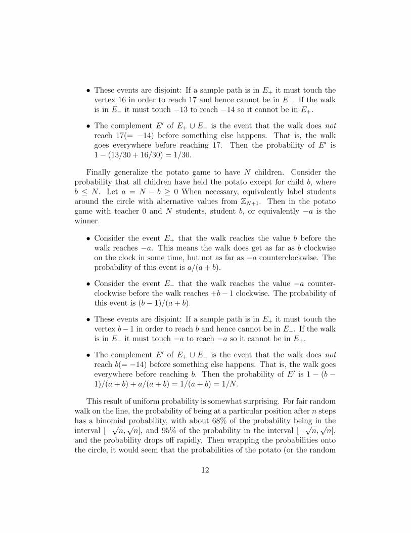
Figure 1: A simulation of the potato game with the teacher at position 0, 30students around the circle and 50 passes of the potato.

10

2, that is, in the potato game with teacher 0 and 3 students, the student 2(equivalently −2) is the winner.

Unfold the circle and use the theorem on ruin probabilities for a fair walkstarting at 0 and terminating with ruin at −a or victory at b

P [Tτ = b] =a

a+ band P [Tτ = −a] =

b

a+ b.

• Consider the event E+ that the walk reaches the value +2 before thewalk reaches −1. This means the walk does get as far as 2 clockwiseon the clock in some time, but not as far as −1 counterclockwise. Theprobability of this event is 1/3.

• Consider the event E− that the walk reaches the value −2 counter-clockwise before the walk reaches +1 clockwise. The probability of thisevent is 1/3.

• These events are disjoint: If a sample point is in E+ it must touch thevertex 1 and hence cannot be in E−. If the walk is in E− it must touch−1 so it cannot be in E+.

• The complement E ′ of E+∪E− is the event that the walk does not reach2 before something else happens. That is, the walk goes everywherebefore reaching 2. Then the probability of E ′ is 1− (1/3 + 1/3) = 1/3.

Now consider the original potato game with teacher 0 and 30 childrenand specifically consider the probability that all children are covered exceptfor child 17, for example. That is, in the potato game with teacher 0 and30 students, student 17 (equivalently −14) is the winner. The example usesstudent 17 because this position is not symmetric with respect to the teacher.

• Consider the event E+ that the walk reaches the value +17 before thewalk reaches −13. This means the walk does get as far as 17 clockwiseon the clock in some time, but not as far as−13(= 18) counterclockwise.The probability of this event is 13/30.

• Consider the event E− that the walk reaches the value −14 counter-clockwise before the walk reaches +16 clockwise. The probability ofthis event is 16/30.

11

• These events are disjoint: If a sample path is in E+ it must touch thevertex 16 in order to reach 17 and hence cannot be in E−. If the walkis in E− it must touch −13 to reach −14 so it cannot be in E+.

• The complement E ′ of E+ ∪ E− is the event that the walk does notreach 17(= −14) before something else happens. That is, the walkgoes everywhere before reaching 17. Then the probability of E ′ is1− (13/30 + 16/30) = 1/30.

Finally generalize the potato game to have N children. Consider theprobability that all children have held the potato except for child b, whereb ≤ N . Let a = N − b ≥ 0 When necessary, equivalently label studentsaround the circle with alternative values from ZN+1. Then in the potatogame with teacher 0 and N students, student b, or equivalently −a is thewinner.

• Consider the event E+ that the walk reaches the value b before thewalk reaches −a. This means the walk does get as far as b clockwiseon the clock in some time, but not as far as −a counterclockwise. Theprobability of this event is a/(a+ b).

• Consider the event E− that the walk reaches the value −a counter-clockwise before the walk reaches +b− 1 clockwise. The probability ofthis event is (b− 1)/(a+ b).

• These events are disjoint: If a sample path is in E+ it must touch thevertex b− 1 in order to reach b and hence cannot be in E−. If the walkis in E− it must touch −a to reach −a so it cannot be in E+.

• The complement E ′ of E+ ∪ E− is the event that the walk does notreach b(= −14) before something else happens. That is, the walk goeseverywhere before reaching b. Then the probability of E ′ is 1 − (b −1)/(a+ b) + a/(a+ b) = 1/(a+ b) = 1/N .

This result of uniform probability is somewhat surprising. For fair randomwalk on the line, the probability of being at a particular position after n stepshas a binomial probability, with about 68% of the probability being in theinterval [−

√n,√n], and 95% of the probability in the interval [−

√n,√n],

and the probability drops off rapidly. Then wrapping the probabilities ontothe circle, it would seem that the probabilities of the potato (or the random

12

walk) passing through the symmetrical adjacent positions 1 and 30 shouldbe relatively large and probability of being at positions 15 and 16 oppositethe teacher should be relatively small. At first glance, it would seem thatstudents 1 and 30 adjacent to the teacher will seldom win and that positions15 or 16 should have the highest probability of winning. However, the gamestops at a random time, after visiting all but one position, not a fixed time.The next section will show that the expected time is 435 steps. After 400steps, the standard deviation of the fair random walk is 20, and wrappingthe random walk onto the circle will cover the circle. Some sample paths willstay on one side of the teacher and then positions 1 or 30 can still win. Somesample paths will oscillate back and forth across the teacher’s position, as inthe figure, and positions 15 or 16 can win.

The interpretation as Markov Processes and Martin-gales

The fortune in the coin-tossing game is the first and simplest encounter withtwo of the most important ideas in modern probability theory.

We can interpret the fortune in our gambler’s coin-tossing game as aMarkov process. That is, at successive times the process is in variousstates. The states are the values of the fortune. The probability of passingfrom one state at the current time t to another state at time t+1 is completelydetermined by the present state. That is, for our coin-tossing game

P [Tt+1 = x+ 1|Tt = x] = p

P [Tt+1 = x− 1|Tt = x] = q

P [Tt+1 = y|Tt = x] = 0 for all y 6= x+ 1, x− 1

The most important property of a Markov process is that the probability ofbeing in the next state is completely determined by the current state and notthe history of how the process arrived at the current state. In that sense, weoften say that a Markov process is memory-less.

We can also note the fair coin-tossing game with p = 1/2 = q is a mar-tingale. That is, the expected value of the process at the next step is thecurrent value. Using expectation for estimation, the best estimate we haveof the gambler’s fortune at the next step is the current fortune:

E [Tn+1|Tn = x] = (x+ 1)(1/2) + (x− 1)(1/2) = x.

13

This characterizes a fair game, after the next step, one can neither expectto be richer or poorer. Note that the coin-tossing games with p 6= q do nothave this property.

Sources

This section is adapted from W. Feller, in Introduction to Probability Theoryand Applications, Volume I, Chapter XIV, page 342, [1]. Some material isadapted from [3] and [2]. Steele has an excellent discussion at about thesame level as here, but with a slightly more rigorous approach to solving thedifference equations. He also gives more information about the fact that theduration is almost surely finite, showing that all moments of the durationare finite. Karlin and Taylor give a treatment of the ruin problem by directapplication of Markov chain analysis, which is not essentially different, butpoints to greater generality.

Algorithms, Scripts, Simulations

Algorithm

The goal is to simulate the probability function for ruin with a given startingvalue. First set the probability p, number of Bernoulli trials n, and numberof experiments k. Set the ruin and victory values r and v, the boundariesfor the random walk. For each starting value from ruin to victory, fill ann × k matrix with the Bernoulli random variables. Languages with multi-dimensional arrays keeps the data in a three-dimensional array of size n ×k × (v − r + 1). Cumulatively sum the Bernoulli random variables to createthe fortune or random walk. For each starting value, for each random walkor fortune path, find the step where ruin or victory is encountered. For eachstarting value, find the proportion of fortunes encountering ruin. Finally,find a least squares linear fit of the ruin probabilities as a function of thestarting value.

14

Scripts

Geogebra Geogebra script for ruin probabilities

R R script for ruin probabilities

1

2 p <- 0.5

3 n <- 150

4 k <- 60

5

6 victory <- 10

7 # top boundary for random walk

8 ruin <- -10

9 # bottom boundary for random walk

10 interval <- victory - ruin + 1

11

12 winLose <- 2 * (array( 0+( runif(n*k*interval) <= p), dim=

c(n,k,

13 interval))) - 1

14 # 0+ coerces Boolean to numeric

15 totals <- apply( winLose , 2:3, cumsum)

16 # the second argument ‘‘2:3’’ means column -wise in each

panel

17 start <- outer( array(1, dim=c(n+1,k)), ruin:victory , "*"

)

18

19 paths <- array( 0 , dim=c(n+1, k, interval) )

20 paths [2:(n+1), 1:k, 1: interval] <- totals

21 paths <- paths + start

22

23 hitVictory <- apply(paths , 2:3, (function(x)match(victory

,x, nomatch=n+2)));

24 hitRuin <- apply(paths , 2:3, (function(x)match(ruin ,

x, nomatch=n+2)));

25 # the second argument ‘‘2:3’’ means column -wise in each

panel

26 # If no ruin or victory on a walk , nomatch=n+2 sets the

hitting

27 # time to be two more than the number of steps , one more

than

28 # the column length. Without the nomatch option , get NA

which

29 # works poorly with the comparison hitRuin < hitVictory

next.

30

15

31 probRuinBeforeVictory <-

32 apply( (hitRuin < hitVictory), 2,

33 (function(x)length (( which(x,arr.ind=FALSE)))) )/k

34

35 startValues <- (ruin:victory);

36 ruinFunction <- lm(probRuinBeforeVictory ~ startValues)

37 # lm is the R function for linear models , a more general

view of

38 # least squares linear fitting for response ~ terms

39 cat(sprintf("Ruin function Intercept: %f \n",

coefficients(ruinFunction)[1] ))

40 cat(sprintf("Ruin function Slope: %f \n", coefficients(

ruinFunction)[2] ))

41

42 plot(startValues , probRuinBeforeVictory);

43 abline(ruinFunction)

44

45

Octave Octave script for ruin probabilities

1 p = 0.5;

2 n = 150;

3 k = 60;

4

5 victory = 10;

6 # top boundary for random walk

7 ruin = -10;

8 # bottom boundary for random walk

9

10 probRuinBeforeVictory = zeros(1, victory -ruin +1);

11 for start = ruin:victory

12

13 winLose = 2 * (rand(n,k) <= p) - 1;

14 # -1 for Tails , 1 for Heads

15 totals = cumsum(winLose);

16 # -n..n (every other integer) binomial rv sample

17

18 paths = [zeros(1,k); totals] + start;

19 victoryOrRuin = zeros(1,k);

20 for j = 1:k

21 hitVictory = find(paths(:,j) >= victory);

22 hitRuin = find(paths(:,j) <= ruin);

23 if ( !rows(hitVictory) && !rows(hitRuin) )

16

24 # no victory , no ruin

25 # do nothing

26 elseif ( rows(hitVictory) && !rows(hitRuin) )

27 # victory , no ruin

28 victoryOrRuin(j) = hitVictory (1);

29 elseif ( !rows(hitVictory) && rows(hitRuin) )

30 # no victory , but hit ruin

31 victoryOrRuin(j) = -hitRuin (1);

32 else # ( rows(hitvictory) && rows(hitruin) )

33 # victory and ruin

34 if ( hitVictory (1) < hitRuin (1) )

35 victoryOrRuin(j) = hitVictory (1);

36 # code hitting victory

37 else

38 victoryOrRuin(j) = -hitRuin (1);

39 # code hitting ruin as negative

40 endif

41 endif

42 endfor

43

44 probRuinBeforeVictory(start + (-ruin +1)) = sum(

victoryOrRuin < 0 )/k;

45 # probRuinBeforeVictory

46 endfor

47

48 function coeff = least_square (x,y)

49 n = length(x);

50 A = [x ones(n,1)];

51 coeff = A\y;

52 plot(x,y,’x’);

53 hold on

54 interv = [min(x) max(x)];

55 plot(interv ,coeff (1)*interv+coeff (2));

56 end

57

58 rf = least_square(transpose( ruin : victory ), transpose(

probRuinBeforeVictory));

59 disp("Ruin function Intercept:"), disp(rf(2))

60 disp("Ruin function Slope:"), disp(rf(1))

61 hold off

62

63

17

Perl Perl PDL script for ruin probabilities

1 use PDL:: NiceSlice;

2

3 $p = 0.5;

4 $n = 150;

5 $k = 60;

6 $victory = 10;

7 $ruin = -10;

8 $interval = $victory - $ruin + 1;

9 $winLose = 2 * ( random( $k, $n, $interval ) <= $p ) -

1;

10 $totals = ( cumusumover $winLose ->xchg( 0, 1 ) )->

transpose;

11 $start = zeroes( $k , $n + 1, $interval )->zlinvals(

$ruin , $victory );

12

13 $paths = zeroes( $k , $n + 1, $interval );

14

15 # use PDL:NiceSlice on next line

16 $paths ( 0 : ( $k - 1 ), 1 : $n , 0 : ( $interval - 1 ) )

.= $totals;

17

18 # Note the use of the concat operator here.

19 $paths = $paths + $start;

20 $hitVictory = $paths ->setbadif( $paths < $victory );

21 $hitRuin = $paths ->setbadif( $paths > $ruin );

22

23 $victoryIndex =

24 ( $hitVictory ( ,, : )->xchg( 0, 1 )->minimum_ind )

25 ->inplace ->setbadtoval( $n + 1 );

26 $ruinIndex =

27 ( $hitRuin ( ,, : )->xchg( 0, 1 )->maximum_ind )

28 ->inplace ->setbadtoval( $n + 1 );

29

30 $probRuinBeforeVictory = sumover( float( $ruinIndex <

$victoryIndex ) ) / $k;

31

32 use PDL::Fit:: Linfit;

33 $x = zeroes($interval)->xlinvals( $ruin , $victory );

34 $fitFuncs = cat ones($interval), $x;

35 ( $ruinFunction , $coeffs ) = linfit1d

$probRuinBeforeVictory , $fitFuncs;

36 print "Ruin function Intercept:", $coeffs (0), "\n";

37 print "Ruin function Slope:", $coeffs (1), "\n";

38

18

39

SciPy Scientific Python script for ruin probabilities

1 import scipy

2

3 p = 0.5

4 n = 150

5 k = 60

6 victory = 10;

7 ruin = -10;

8 interval = victory - ruin + 1;

9

10 winLose = 2*( scipy.random.random ((n,k,interval)) <= p )

- 1

11 totals = scipy.cumsum(winLose , axis = 0)

12

13 start = scipy.multiply.outer( scipy.ones((n+1,k), dtype=

int), scipy.arange(ruin , victory+1, dtype=int))

14 paths = scipy.zeros ((n+1,k,interval), dtype=int)

15 paths[ 1:n+1, :,:] = totals

16 paths = paths + start

17

18 def match(a,b,nomatch=None):

19 return b.index(a) if a in b else nomatch

20 # arguments: a is a scalar , b is a python list , value of

nomatch is scalar

21 # returns the position of first match of its first

argument in its second argument

22 # but if a is not there , returns the value nomatch

23 # modeled on the R function "match", but with less

generality

24

25 hitVictory = scipy.apply_along_axis(lambda x:( match(

victory ,x.tolist (),nomatch=n+2)), 0, paths)

26 hitRuin = scipy.apply_along_axis(lambda x:match(ruin ,x.

tolist (),nomatch=n+2), 0, paths)

27 # If no ruin or victory on a walk , nomatch=n+2 sets the

hitting

28 # time to be two more than the number of steps , one more

than

29 # the column length.

30

19

31 probRuinBeforeVictory = scipy.mean( (hitRuin < hitVictory

), axis =0)

32 # note that you can treat the bool’s as binary data!

33

34 ruinFunction = scipy.polyfit( scipy.arange(ruin , victory

+1, dtype=int), probRuinBeforeVictory , 1)

35 print "Ruin function Intercept:", ruinFunction [1];

36 print "Ruin function Slope:", ruinFunction [0];

37 # should return a slope near -1/(victory -ruin) and an

intercept near 0.5

38

39

Problems to Work for Understanding

1. Consider the ruin probabilities qT0 as a function of T0. What is thedomain of qT0 ? What is the range of qT0 ? Explain heuristically whyqT0 is decreasing as a function of T0.

2. Show that power functions have the property that the ratio of successivedifferences is constant.

3. Show the sequence [(q/p)n− 1]/n is an increasing sequence for 0 < p <1/2 < q < 1.

4. In a random walk starting at the origin find the probability that thepoint a > 0 will be reached before the point −b < 0.

5. James Bond wants to ruin the casino at Monte Carlo by consistentlybetting 1 Euro on Red at the roulette wheel. The probability of Bondwinning at one turn in this game is 18/38 ≈ 0.474. James Bond, beingAgent 007, is backed by the full financial might of the British Empire,and so can be considered to have unlimited funds. Approximately how

20

much money should the casino have to start with so that Bond hasonly a “one-in-a-million” chance of ruining the casino?

6. A gambler starts with $2 and wants to win $2 more to get to a total of$4 before being ruined by losing all his money. He plays a coin-flippinggame, with a coin that changes with his fortune.

(a) If the gambler has $2 he plays with a coin that gives probabilityp = 1/2 of winning a dollar and probability q = 1/2 of losing adollar.

(b) If the gambler has $3 he plays with a coin that gives probabilityp = 1/4 of winning a dollar and probability q = 3/4 of losing adollar.

(c) If the gambler has $1 he plays with a coin that gives probabilityp = 3/4 of winning a dollar and probability q = 1/4 of losing adollar.

Use “first step analysis” to write three equations in three unknowns(with two additional boundary conditions) that give the probabilitythat the gambler will be ruined. Solve the equations to find the ruinprobability.

7. A gambler plays a coin flipping game in which the probability of win-ning on a flip is p = 0.4 and the probability of losing on a flip isq = 1 − p = 0.6. The gambler wants to reach the victory level of $16before being ruined with a fortune of $0. The gambler starts with $8,bets $2 on each flip when the fortune is $6, $8, $10 and bets $4 whenthe fortune is $4 or $12 Compute the probability of ruin in this game.

8. Prove: In a random walk starting at the origin the probability to reachthe point a > 0 before returning to the origin equals p(1− q1).

9. Prove: In a random walk starting at a > 0 the probability to reach theorigin before returning to the starting point equals qqa−1.

10. In the simple case p = 1/2 = q, conclude from the preceding problem:In a random walk starting at the origin, the number of visits to thepoint a > 0 that take place before the first return to the origin hasa geometric distribution with ratio 1 − qqa−1. (Why is the conditionq ≥ p necessary?)

21

11. (a) Draw a sample path of a random walk (with p = 1/2 = q) startingfrom the origin where the walk visits the position 5 twice beforereturning to the origin.

(b) Using the results from the previous problems, it can be shownwith careful but elementary reasoning that the number of timesN that a random walk (p = 1/2 = q) reaches the value a a totalof n times before returning to the origin is a geometric randomvariable with probability

P [N = n] =

(1

2a

)n(1− 1

2a

).

Compute the expected number of visits E [N ] to level a.

(c) Compare the expected number of visits of a random walk (withp = 1/2 = q) to the value 1,000,000 before returning to the originand to the level 10 before returning to the origin.

12. This problem is adapted from Stochastic Calculus and Financial Ap-plications by J. Michael Steele, Springer, New York, 2001, Chapter 1,Section 1.6, page 9. Information on buy-backs is adapted from investor-words.com. This problem suggests how results on biased random walkscan be worked into more realistic models.

Consider a naive model for a stock that has a support level of $20/sharebecause of a corporate buy-back program. (This means the companywill buy back stock if shares dip below $20 per share. In the caseof stocks, this reduces the number of shares outstanding, giving eachremaining shareholder a larger percentage ownership of the company.This is usually considered a sign that the company’s management isoptimistic about the future and believes that the current share price isundervalued. Reasons for buy-backs include putting unused cash to use,raising earnings per share, increasing internal control of the company,and obtaining stock for employee stock option plans or pension plans.)Suppose also that the stock price moves randomly with a downwardbias when the price is above $20, and randomly with an upward biaswhen the price is below $20. To make the problem concrete, we letSn denote the stock price at time n, and we express our stock support

22

hypothesis by the assumptions that

P [Sn+1 = 21|Sn = 20] = 9/10

P [Sn+1 = 19|Sn = 20] = 1/10

We then reflect the downward bias at price levels above $20 by requiringthat for k > 20:

P [Sn+1 = k + 1|Sn = k] = 1/3

P [Sn+1 = k − 1|Sn = k] = 2/3.

We then reflect the upward bias at price levels below $20 by requiringthat for k < 20:

P [Sn+1 = k + 1|Sn = k] = 2/3

P [Sn+1 = k − 1|Sn = k] = 1/3

Using the methods of “single-step analysis” calculate the expected timefor the stock to fall from $25 through the support level all the way downto $18. (Because of the varying parameters there is no way to solvethis problem using formulas. Instead you will have to go back to basicprinciples of single-step or first-step analysis to solve the problem.)

13. Modify the ruin probability scripts to perform simulations of the ruincalculations in the table in the section Some Calculations for Illustra-tion and compare the results.

14. Do some simulations of the coin-flipping game, varying p and the startvalue. How does the value of p affect the experimental probability ofvictory and ruin?

15. Modify the simulations by changing the value of p and comparing theexperimental results for each starting value to the theoretical ruin func-tion.

23

Reading Suggestion:

References

[1] William Feller. An Introduction to Probability Theory and Its Applica-tions, Volume I, volume I. John Wiley and Sons, third edition, 1973. QA273 F3712.

[2] S. Karlin and H. Taylor. A Second Course in Stochastic Processes. Aca-demic Press, 1981.

[3] J. Michael Steele. Stochastic Calculus and Financial Applications.Springer-Verlag, 2001. QA 274.2 S 74.

Outside Readings and Links:

1. Virtual Labs in Probability Games of Chance. Scroll down and selectthe Red and Black Experiment (marked in red in the Applets Section.Read the description since the scenario is slightly different but equiva-lent to the description above.)

2. University of California, San Diego, Department of Mathematics, A.M.Garsia A java applet that simulates how long it takes for a gambler togo broke. You can control how much money you and the casino startwith, the house odds, and the maximum number of games. Results area graph and a summary table. Submitted by Matt Odell, September8, 2003.

3. Eric Weisstein, World of Mathematics A good description of gambler’sruin, martingale and many other coin tossing and dice problems andvarious probability problems Submitted by Yogesh Makkar, September16th 2003.

24

I check all the information on each page for correctness and typographicalerrors. Nevertheless, some errors may occur and I would be grateful if you wouldalert me to such errors. I make every reasonable effort to present current andaccurate information for public use, however I do not guarantee the accuracy ortimeliness of information on this website. Your use of the information from thiswebsite is strictly voluntary and at your risk.

I have checked the links to external sites for usefulness. Links to externalwebsites are provided as a convenience. I do not endorse, control, monitor, orguarantee the information contained in any external website. I don’t guaranteethat the links are active at all times. Use the links here with the same caution asyou would all information on the Internet. This website reflects the thoughts, in-terests and opinions of its author. They do not explicitly represent official positionsor policies of my employer.

Information on this website is subject to change without notice.

Steve Dunbar’s Home Page, http://www.math.unl.edu/~sdunbar1Email to Steve Dunbar, sdunbar1 at unl dot edu

Last modified: Processed from LATEX source on September 28, 2017

25