Topaze Guided Session #4 - KAPPA Eng
16
Ecrin v4.20 - Doc v4.20.01 - © KAPPA 1988-2011 Topaze Guided Session #4 • TopGS04 - 1/16 Topaze Guided Session #4 A01 • Introduction This guided session is an introduction to the basic facilities of the reservoir production profile option in Topaze. Topaze can be used in two distinct manners: - Match field profile: A target field profile is defined and the program automatically determines the necessary drilling schedule, on a monthly basis, to meet the target. - Build field profile: The user defines the drilling schedule, and the field production is built accordingly. This session will illustrate both approaches. B01 • Oil – Water Drive Case: Build Field Profile B01.1 • Starting a new Topaze Project Click on New Document, set the document structure to multi-well and check the option ‘Generate the production profile’, as shown below: Fig. B01 • Multi-well new document
Transcript of Topaze Guided Session #4 - KAPPA Eng
Ecrin v4.20 - Doc v4.20.01 - © KAPPA 1988-2011 Topaze Guided Session #4 • TopGS04 - 1/16
Topaze Guided Session #4
A01 • Introduction
This guided session is an introduction to the basic facilities of the reservoir production profile
option in Topaze. Topaze can be used in two distinct manners:
- Match field profile: A target field profile is defined and the program automatically
determines the necessary drilling schedule, on a monthly basis, to meet the target.
- Build field profile: The user defines the drilling schedule, and the field production is built
accordingly.
This session will illustrate both approaches.
B01 • Oil – Water Drive Case: Build Field Profile
B01.1 • Starting a new Topaze Project
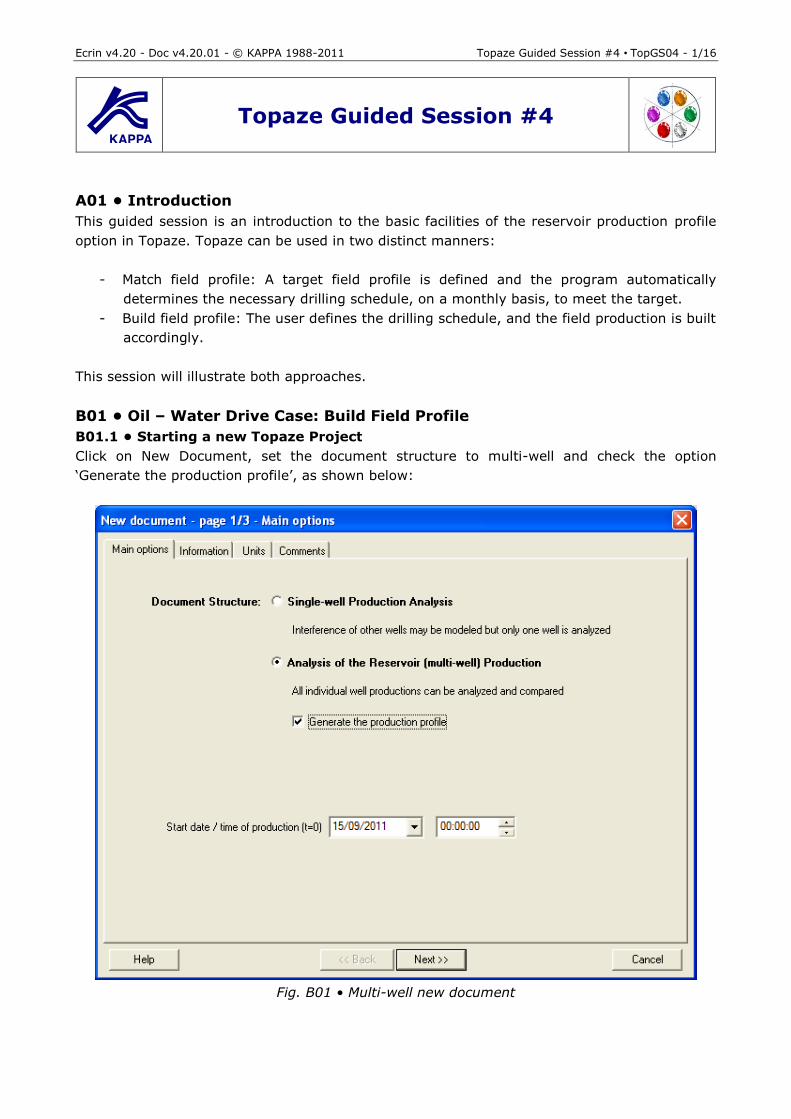
Click on New Document, set the document structure to multi-well and check the option
‘Generate the production profile’, as shown below:
Fig. B01 • Multi-well new document
Ecrin v4.20 - Doc v4.20.01 - © KAPPA 1988-2011 Topaze Guided Session #4 • TopGS04 - 2/16
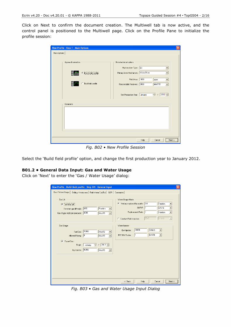
Click on Next to confirm the document creation. The Multiwell tab is now active, and the
control panel is positioned to the Multiwell page. Click on the Profile Pane to initialize the
profile session:
Fig. B02 • New Profile Session
Select the ‘Build field profile’ option, and change the first production year to January 2012.
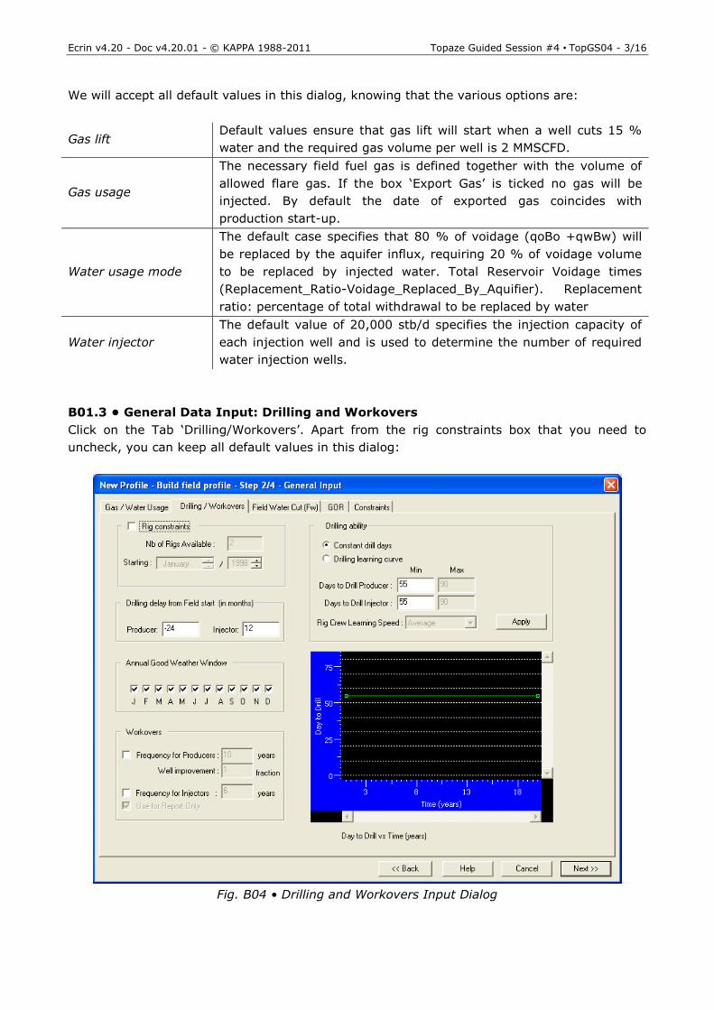
B01.2 • General Data Input: Gas and Water Usage
Click on ‘Next’ to enter the ‘Gas / Water Usage’ dialog:
Fig. B03 • Gas and Water Usage Input Dialog
Ecrin v4.20 - Doc v4.20.01 - © KAPPA 1988-2011 Topaze Guided Session #4 • TopGS04 - 3/16
We will accept all default values in this dialog, knowing that the various options are:
Gas lift Default values ensure that gas lift will start when a well cuts 15 %
water and the required gas volume per well is 2 MMSCFD.
Gas usage
The necessary field fuel gas is defined together with the volume of
allowed flare gas. If the box ‘Export Gas’ is ticked no gas will be
injected. By default the date of exported gas coincides with
production start-up.
Water usage mode
The default case specifies that 80 % of voidage (qoBo +qwBw) will
be replaced by the aquifer influx, requiring 20 % of voidage volume
to be replaced by injected water. Total Reservoir Voidage times
(Replacement_Ratio-Voidage_Replaced_By_Aquifier). Replacement
ratio: percentage of total withdrawal to be replaced by water
Water injector
The default value of 20,000 stb/d specifies the injection capacity of
each injection well and is used to determine the number of required
water injection wells.
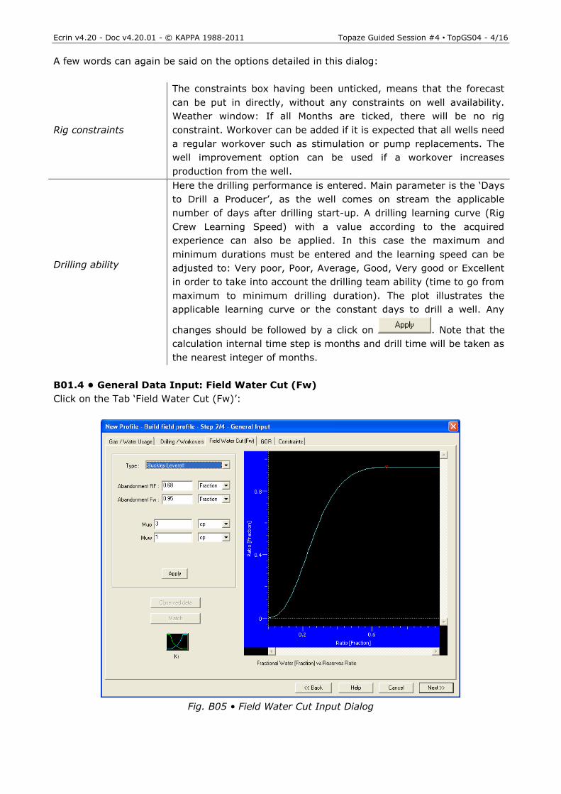
B01.3 • General Data Input: Drilling and Workovers
Click on the Tab ‘Drilling/Workovers’. Apart from the rig constraints box that you need to
uncheck, you can keep all default values in this dialog:
Fig. B04 • Drilling and Workovers Input Dialog
Ecrin v4.20 - Doc v4.20.01 - © KAPPA 1988-2011 Topaze Guided Session #4 • TopGS04 - 4/16
A few words can again be said on the options detailed in this dialog:
Rig constraints
The constraints box having been unticked, means that the forecast
can be put in directly, without any constraints on well availability.
Weather window: If all Months are ticked, there will be no rig
constraint. Workover can be added if it is expected that all wells need
a regular workover such as stimulation or pump replacements. The
well improvement option can be used if a workover increases
production from the well.
Drilling ability
Here the drilling performance is entered. Main parameter is the ‘Days
to Drill a Producer’, as the well comes on stream the applicable
number of days after drilling start-up. A drilling learning curve (Rig
Crew Learning Speed) with a value according to the acquired
experience can also be applied. In this case the maximum and
minimum durations must be entered and the learning speed can be
adjusted to: Very poor, Poor, Average, Good, Very good or Excellent
in order to take into account the drilling team ability (time to go from
maximum to minimum drilling duration). The plot illustrates the
applicable learning curve or the constant days to drill a well. Any
changes should be followed by a click on . Note that the
calculation internal time step is months and drill time will be taken as
the nearest integer of months.
B01.4 • General Data Input: Field Water Cut (Fw)
Click on the Tab ‘Field Water Cut (Fw)’:
Fig. B05 • Field Water Cut Input Dialog
Ecrin v4.20 - Doc v4.20.01 - © KAPPA 1988-2011 Topaze Guided Session #4 • TopGS04 - 5/16
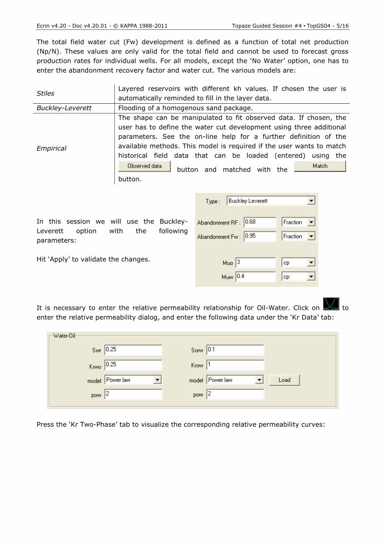
The total field water cut (Fw) development is defined as a function of total net production
(Np/N). These values are only valid for the total field and cannot be used to forecast gross
production rates for individual wells. For all models, except the ‘No Water’ option, one has to
enter the abandonment recovery factor and water cut. The various models are:
Stiles Layered reservoirs with different kh values. If chosen the user is
automatically reminded to fill in the layer data.
Buckley-Leverett Flooding of a homogenous sand package.
Empirical
The shape can be manipulated to fit observed data. If chosen, the
user has to define the water cut development using three additional
parameters. See the on-line help for a further definition of the
available methods. This model is required if the user wants to match
historical field data that can be loaded (entered) using the
button and matched with the
button.
In this session we will use the Buckley-
Leverett option with the following
parameters:
Hit ‘Apply’ to validate the changes.
It is necessary to enter the relative permeability relationship for Oil-Water. Click on to
enter the relative permeability dialog, and enter the following data under the ‘Kr Data’ tab:
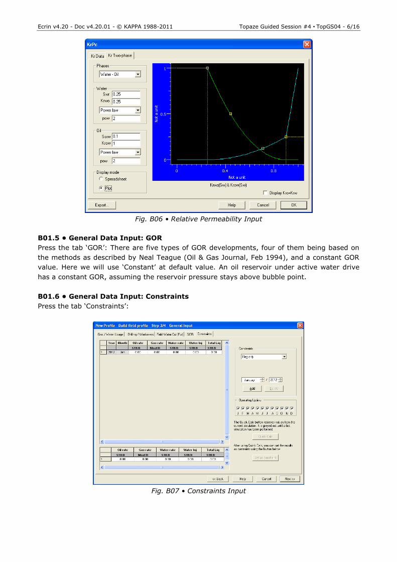
Press the ‘Kr Two-Phase’ tab to visualize the corresponding relative permeability curves:
Ecrin v4.20 - Doc v4.20.01 - © KAPPA 1988-2011 Topaze Guided Session #4 • TopGS04 - 6/16
Fig. B06 • Relative Permeability Input
B01.5 • General Data Input: GOR
Press the tab ‘GOR’: There are five types of GOR developments, four of them being based on
the methods as described by Neal Teague (Oil & Gas Journal, Feb 1994), and a constant GOR
value. Here we will use ‘Constant’ at default value. An oil reservoir under active water drive
has a constant GOR, assuming the reservoir pressure stays above bubble point.
B01.6 • General Data Input: Constraints
Press the tab ‘Constraints’:
Fig. B07 • Constraints Input
Ecrin v4.20 - Doc v4.20.01 - © KAPPA 1988-2011 Topaze Guided Session #4 • TopGS04 - 7/16
The constraints entered here can correspond to the operational field production limitations due
to logistics and storage, for instance. The following can be specified and modified at any point
in time: oil rate, gas rate, water production, water injection, total liquid rate.
In any Topaze forecast, the governing phase production, Oil or Gas, is driving all the other
phase productions or injections. For this reason, any of the above constraint can be translated
into a constraint on the main phase. This is called the minimum constraint and it is the value
used internally to check the main phase production. Note that at a given time step, this
minimum constraint is a function of Np/N. The minimum constraint can be plotted on the Field
production plot (Well schedule tab). With time, varying colors indicate what constraint is
causing the bottleneck.
Constraints can be handled in 3 ways:
Undefined: When a constraint value is zero, Topaze will ignore it. This constraint will have no
effect on the calculations or the results.
Flag only: In this case the constraints have no impact on the production. In the Tables and
Results sections, those values that violate a constraint are highlighted in red. Note for instance
that in an oil case, if the gas production exceeds the gas constraint, then necessarily the oil
production exceeds the ‘minimum constraint’. So violating a constraint other than the one on
the main phase entails the violation of that main phase ‘minimum constraint’ too. Note that
violated means bigger or equal.
Active: At each time step Topaze calculates the minimum constraint and defers any excess
production to future time steps. In the results/tables Topaze will still highlight what constraints
have been violated or reached, to indicate the bottlenecks. Also, in the Results dialog, Topaze-
Profile will report any deferred production that could not be re-allocated.
We will not impose any constraint here; click on ‘Next’ to move to the next stage of the project
definition – the well profiles.
B01.7 • Well Profiles
The Well Profile facility allows the user to enter new Well Production Profiles or to modify
existing ones. Some defaults profiles (named Producer#1, Gas Injector, Water Injector) are
pre-defined. New well profiles can be defined to be used either for prospective wells (manually
added by the user) or for automatic wells (added by the simulation). Their characteristics -
initial rate, number of declines, decline coefficient - can be modified in this dialog by the user.
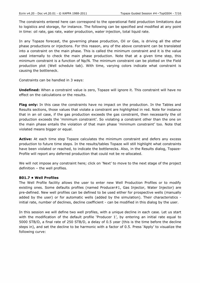
In this session we will define two well profiles, with a unique decline in each case. Let us start
with the modification of the default profile ‘Producer 1’, by entering an initial rate equal to
5000 STB/D, a final rate of 250 STB/D, a delay of 0.5 year (this is the time before the decline
steps in), and set the decline to be harmonic with a factor of 0.5. Press ‘Apply’ to visualize the
following curve:
Ecrin v4.20 - Doc v4.20.01 - © KAPPA 1988-2011 Topaze Guided Session #4 • TopGS04 - 8/16
Fig. B08 • Defining a harmonic decline on Producer 1
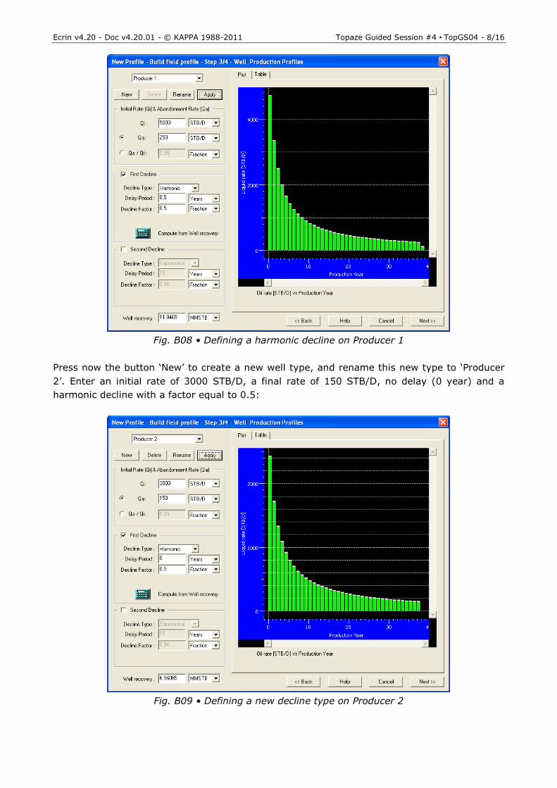
Press now the button ‘New’ to create a new well type, and rename this new type to ‘Producer
2’. Enter an initial rate of 3000 STB/D, a final rate of 150 STB/D, no delay (0 year) and a
harmonic decline with a factor equal to 0.5:
Fig. B09 • Defining a new decline type on Producer 2
Ecrin v4.20 - Doc v4.20.01 - © KAPPA 1988-2011 Topaze Guided Session #4 • TopGS04 - 9/16
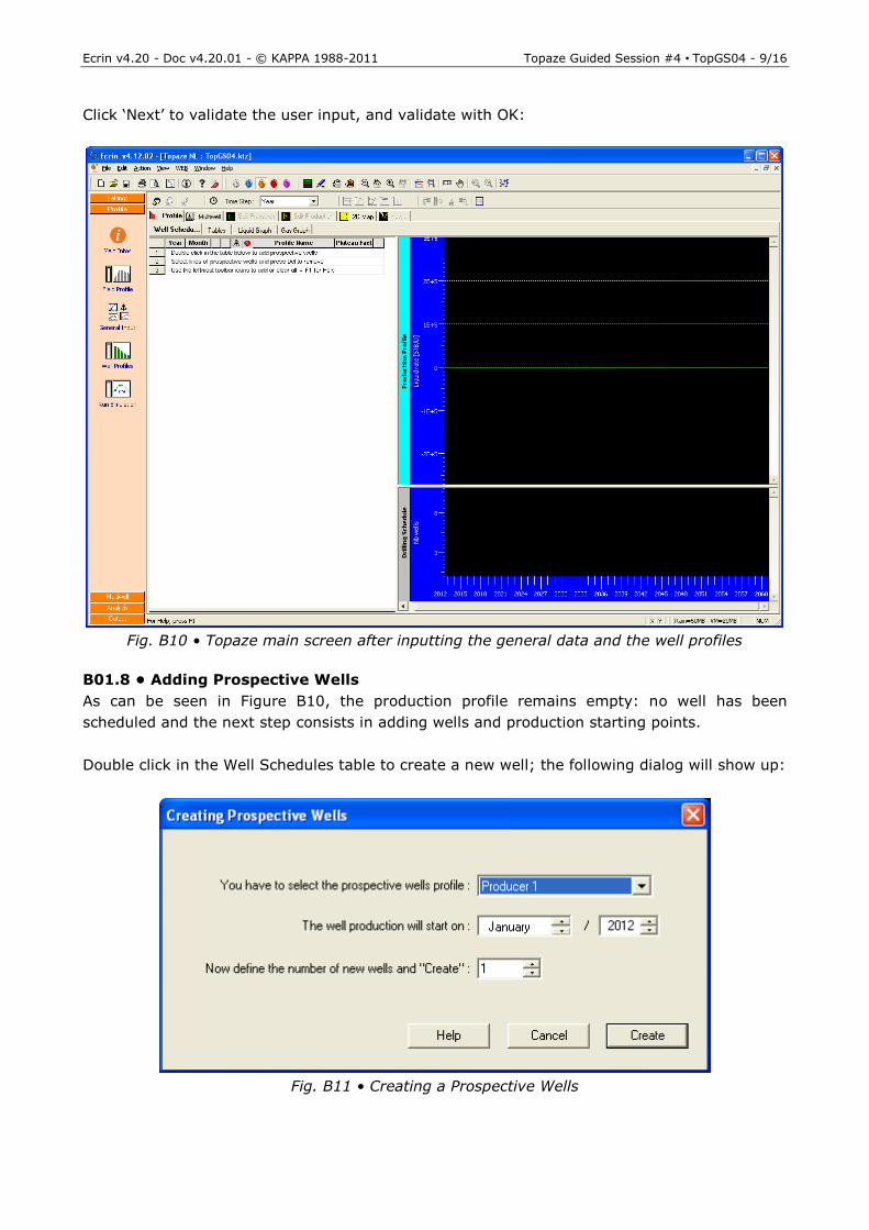
Click ‘Next’ to validate the user input, and validate with OK:
Fig. B10 • Topaze main screen after inputting the general data and the well profiles
B01.8 • Adding Prospective Wells
As can be seen in Figure B10, the production profile remains empty: no well has been
scheduled and the next step consists in adding wells and production starting points.
Double click in the Well Schedules table to create a new well; the following dialog will show up:
Fig. B11 • Creating a Prospective Wells
Ecrin v4.20 - Doc v4.20.01 - © KAPPA 1988-2011 Topaze Guided Session #4 • TopGS04 - 10/16
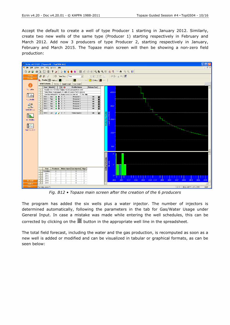
Accept the default to create a well of type Producer 1 starting in January 2012. Similarly,
create two new wells of the same type (Producer 1) starting respectively in February and
March 2012. Add now 3 producers of type Producer 2, starting respectively in January,
February and March 2015. The Topaze main screen will then be showing a non-zero field
production:
Fig. B12 • Topaze main screen after the creation of the 6 producers
The program has added the six wells plus a water injector. The number of injectors is
determined automatically, following the parameters in the tab for Gas/Water Usage under
General Input. In case a mistake was made while entering the well schedules, this can be
corrected by clicking on the button in the appropriate well line in the spreadsheet.
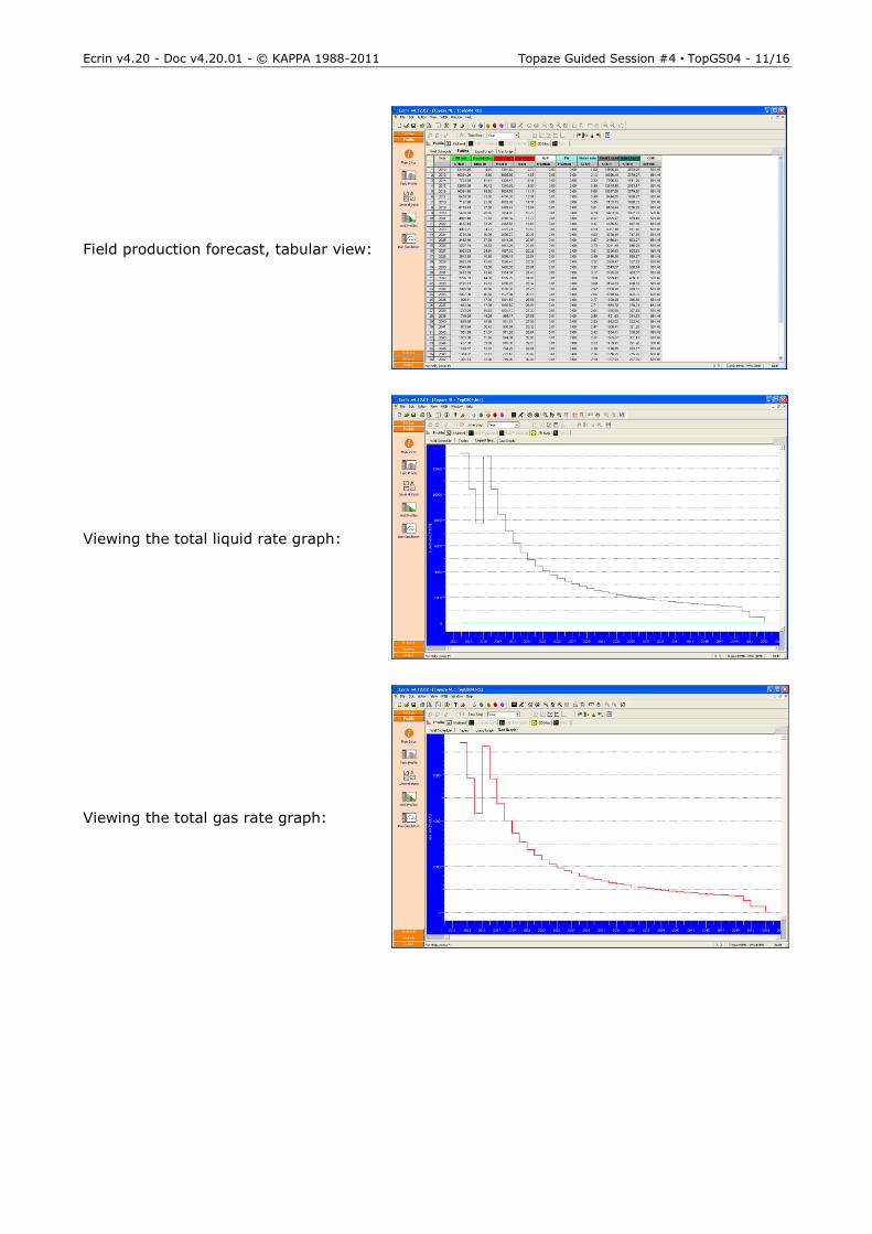
The total field forecast, including the water and the gas production, is recomputed as soon as a
new well is added or modified and can be visualized in tabular or graphical formats, as can be
seen below:
Ecrin v4.20 - Doc v4.20.01 - © KAPPA 1988-2011 Topaze Guided Session #4 • TopGS04 - 11/16
Field production forecast, tabular view:
Viewing the total liquid rate graph:
Viewing the total gas rate graph:
Ecrin v4.20 - Doc v4.20.01 - © KAPPA 1988-2011 Topaze Guided Session #4 • TopGS04 - 12/16
B02 • Oil – Water Drive Case: Match Field Profile
B02.1 • Switching to the Match Field Profile Method
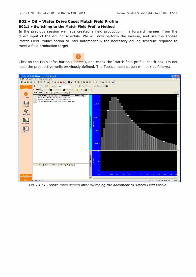
In the previous session we have created a field production in a forward manner, from the
direct input of the drilling schedule. We will now perform the inverse, and use the Topaze
‘Match Field Profile’ option to infer automatically the necessary drilling schedule required to
meet a field production target.
Click on the Main Infos button ( ), and check the ‘Match field profile’ check-box. Do not
keep the prospective wells previously defined. The Topaze main screen will look as follows:
Fig. B13 • Topaze main screen after switching the document to ‘Match Field Profile’
Ecrin v4.20 - Doc v4.20.01 - © KAPPA 1988-2011 Topaze Guided Session #4 • TopGS04 - 13/16
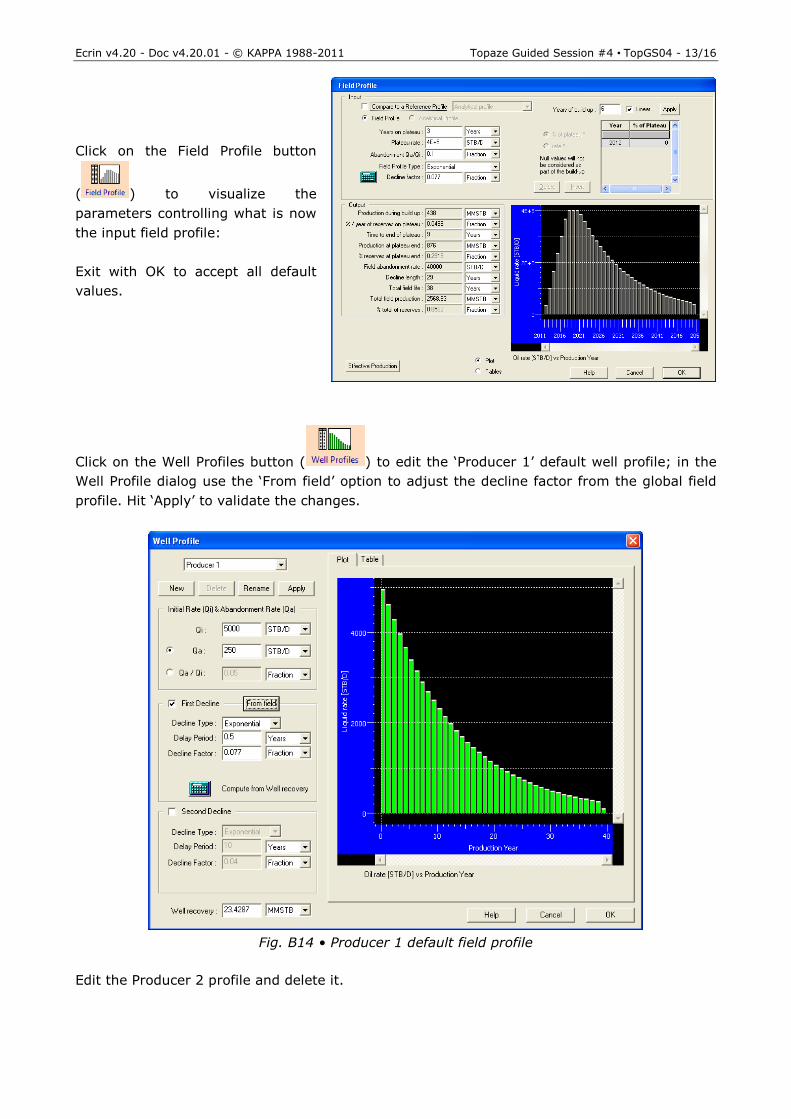
Click on the Field Profile button
( ) to visualize the
parameters controlling what is now
the input field profile:
Exit with OK to accept all default
values.
Click on the Well Profiles button ( ) to edit the ‘Producer 1’ default well profile; in the
Well Profile dialog use the ‘From field’ option to adjust the decline factor from the global field
profile. Hit ‘Apply’ to validate the changes.
Fig. B14 • Producer 1 default field profile
Edit the Producer 2 profile and delete it.

Ecrin v4.20 - Doc v4.20.01 - © KAPPA 1988-2011 Topaze Guided Session #4 • TopGS04 - 14/16
Click now on the Run Simulation ( ) button, and change the final initial rate to 4100
STB/D before to proceed with the Topaze field simulation:
Fig. B15 • Topaze main screen after field simulation
A total of 116 producers and 12 injectors were scheduled by the simulation.
B02.2 • Adding Constraints
Let us now assume that for logistic reasons the total oil rate cannot exceed 350,000 STB/D. To
enter this constraint, click on the General Input button in the Constraints tab, and enter
350,000 STB/D in the Oil rate column for a constraint starting in January 2012:
Keep this constraint as ‘Flag only’ for the time being, and click on OK to visualize it in the field
production graph (click on the option):
Ecrin v4.20 - Doc v4.20.01 - © KAPPA 1988-2011 Topaze Guided Session #4 • TopGS04 - 15/16
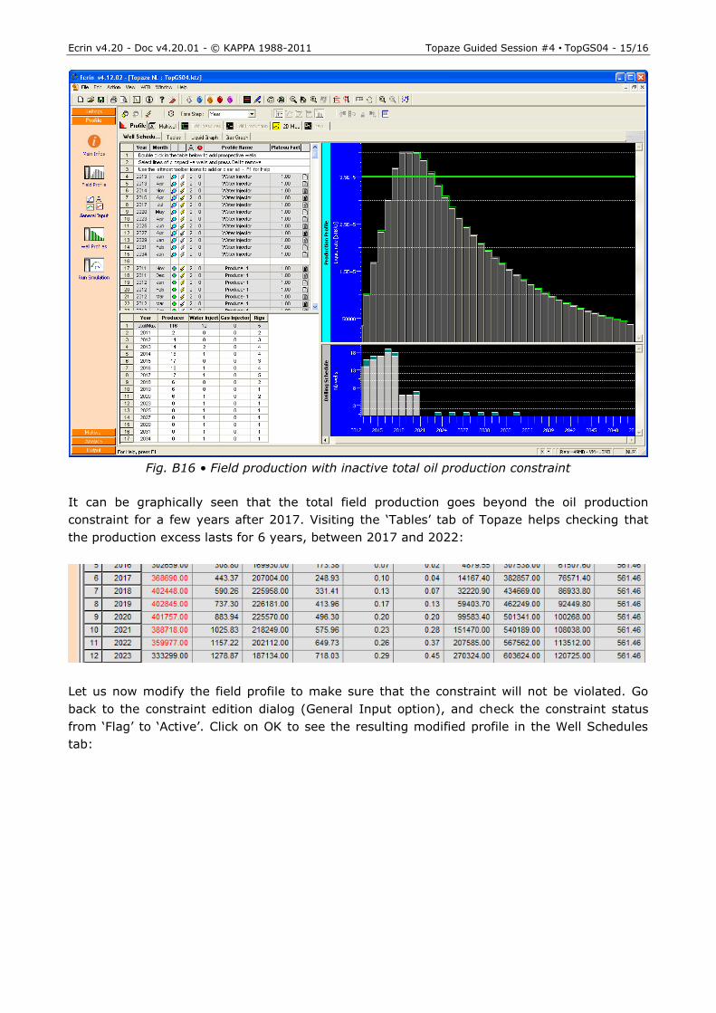
Fig. B16 • Field production with inactive total oil production constraint
It can be graphically seen that the total field production goes beyond the oil production
constraint for a few years after 2017. Visiting the ‘Tables’ tab of Topaze helps checking that
the production excess lasts for 6 years, between 2017 and 2022:
Let us now modify the field profile to make sure that the constraint will not be violated. Go
back to the constraint edition dialog (General Input option), and check the constraint status
from ‘Flag’ to ‘Active’. Click on OK to see the resulting modified profile in the Well Schedules
tab:
Ecrin v4.20 - Doc v4.20.01 - © KAPPA 1988-2011 Topaze Guided Session #4 • TopGS04 - 16/16
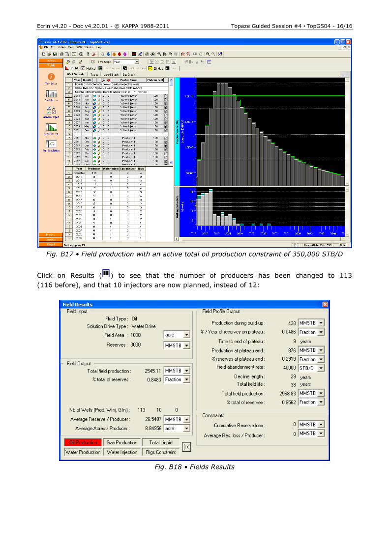
Fig. B17 • Field production with an active total oil production constraint of 350,000 STB/D
Click on Results ( ) to see that the number of producers has been changed to 113
(116 before), and that 10 injectors are now planned, instead of 12:
Fig. B18 • Fields Results