Tool 6: Poverty - Open Knowledge Repository
50
Tool 6: Poverty Equity Issues, Tobacco, and the Poor Richard M. Peck DRAFT USERS : PLEASE PROVIDE FEEDBACK AND COMMENTS TO Joy de Beyer ( [email protected]) and Ayda Yurekli ([email protected]) World Bank, MSN G7-702 1818 H Street NW Washington DC, 20433 USA Fax : (202) 522-3234 Editors: Ayda Yurekli & Joy de Beyer WORLD BANK ECONOMICS OF TOBACCO TOOLKIT Public Disclosure Authorized Public Disclosure Authorized Public Disclosure Authorized Public Disclosure Authorized
Transcript of Tool 6: Poverty - Open Knowledge Repository

Tool 6: Poverty
Equity Issues, Tobacco, and the Poor
Richard M. Peck
DRAFT
USERS : PLEASE PROVIDE FEEDBACK AND COMMENTS TO Joy de Beyer ( [email protected]) and Ayda Yurekli ([email protected]) World Bank, MSN G7-702 1818 H Street NW Washington DC, 20433 USA
Fax : (202) 522-3234
Editors: Ayda Yurekli & Joy de Beyer
WORLD BANK
ECONOMICS OF TOBACCO TOOLKIT
Pub
lic D
iscl
osur
e A
utho
rized
Pub
lic D
iscl
osur
e A
utho
rized
Pub
lic D
iscl
osur
e A
utho
rized
Pub
lic D
iscl
osur
e A
utho
rized
WB456288
Typewritten Text
80579

Equity Issues, Tobacco, and the Poor
ii
Contents
I. Introduction 1
Purpose of this Tool ..................................................................................................... 1 Who Should Use this Tool ........................................................................................... 3 How to Use this Tool ................................................................................................... 3
II. Key Information 5
Definitions ................................................................................................................... 5 Poverty .......................................................................................................... 5 Income ........................................................................................................... 6 Income Quintiles ........................................................................................... 6
Assumptions and Requirements ................................................................................ 10
III. Tobacco Consumption and Expenditures 11
Consider Income and Expenditures ........................................................................... 11 Income Share ............................................................................................... 11 Tobacco Expenditures ................................................................................. 12
Consider Elasticity and Product Quality .................................................................... 12 Income Elasticity ......................................................................................... 12 Luxury Goods .............................................................................................. 13 Calculate Income Elasticity ......................................................................... 14
IV. Tobacco Tax Fairness 15
Define a Regressive Tax ............................................................................................ 15 Determine if a Tax is Regressive ............................................................................... 16
Income Elasticity Less Than Zero ............................................................... 17 Income Elasticity Between Zero and One ................................................... 17
Determine a Tax’s Marginal Value ........................................................................... 18 Price Elasticity............................................................................................. 19 Marginal Progressivity ................................................................................ 21
Examples ................................................................................................................... 23 Example A ................................................................................................... 23 Example B ................................................................................................... 23 Knowledge Required to Conduct an Analysis ............................................. 25
V. Standard of Living 26
Define the Parameters ................................................................................................ 26 Percentage Change in Tobacco Price .......................................................... 26 Prevalence Rate ........................................................................................... 27 Number of Adults per Household ................................................................ 27 Household Tobacco Expenditures ............................................................... 27
Assess the Impact of Higher Tobacco Taxes on Household Expenditures ................ 28 Analyze the Parameters ............................................................................... 29

Equity Issues, Tobacco, and the Poor
iii
An Example ................................................................................................. 30
VI. Poverty and Tobacco-Related Illness 31
Estimate Tobacco-Related Deaths and Disability Adjusted Life Years Lost ............ 32 An Example ................................................................................................. 33
Calculate the Health Impact of Higher Tobacco Taxes ............................................. 33
VII. Tax Incidence 34
Understand How the Burden of Tax is Shifted .......................................................... 34 Examine the Entire Tax System ................................................................................ 35
Obtain an Overview of the Tax System....................................................... 36 Study Income Taxes .................................................................................... 36 Study Excise and Sales Taxes ..................................................................... 36 Study Property Taxes .................................................................................. 37
Determine Net Taxes Paid ......................................................................................... 38 Measure Inequality .................................................................................................... 38 Determine the Pre- and Post-Tax Gini Coefficient .................................................... 39
An Example ................................................................................................. 40 Compute Gini Coefficients with a Spreadsheet ......................................................... 41 Consider a Minimalist Approach ............................................................................... 42
VIII. Conclusion 44
IX. Additional References 45

Equity Issues, Tobacco, and the Poor
iv
List of Tables and Figures
Tables
Table 6.1. Incremental Tax Ratio: ΔRwealthy/ΔRpoor .................................................... 23
Table 6.2. Ratio of Incremental Tax Income Shares: ΔTwealthy/Iwealthy/
ΔTpoor/Ipoor .................................................................................................................. 24
Table 6.3. Impact of Tobacco Taxes on Income ........................................................ 40
Table 6.4. Income Share Difference for Pre-Tax Income .......................................... 41
Table 6.5. Income Share Difference for Post-Tax Income ........................................ 42

Equity Issues, Tobacco, and the Poor
1
I. Introduction
Purpose of this Tool
Currently there are approximately 4 million tobacco related deaths
annually. If present trends continue, by the year 2030 the number of
deaths will soar to about 10 million annual deaths, with 7 million in
low-income countries. However, government action to establish
various tobacco control initiatives can prevent this from happening
and save a significant number of lives. Tobacco control measures
include:
raising tobacco prices by imposing higher excise taxes
advertising and marketing bans and restrictions
clean indoor air provisions.
A 10% tobacco tax could
lower tobacco consumption
by 8% and save 10 million
lives.
Perhaps the most effective tobacco control measure involves
increasing tobacco excise taxes. For instance, if tobacco taxes are
raised worldwide to increase the price of tobacco products by 10
percent, consumption will decline by approximately 8 percent and
about 10 million lives can be saved. It is estimated that most of the
reduction in death (about 90 percent) will occur in low- and middle-
income countries (World Bank Report, 1999).
A popular and valid concern holds that raising tobacco excise taxes
for the purposes of tobacco control imposes an untenable and unfair
burden on the poor. In short, it is argued that higher tobacco excise
taxes increase inequality in the post-tax distribution of income and
reduces the real incomes of a particularly vulnerable group—the
poor. This Tool discusses a number of approaches in which to
examine the validity of this argument. Techniques to analyze the
impact of tobacco consumption and tobacco taxes on the poor are
explained. And analytical methods using country-specific data are
examined so that policy analysts can effectively address concerns
about the poor, tobacco consumption, and tobacco control policies.
Equity Issues, Tobacco, and the Poor
2
According to a variety of measures, there are significant differences
in the health of the wealthy and the poor. The poor experience higher
rates of morbidity and shorter life expectancy, higher rates of infant
mortality, and low birth weights. The relationships between superior
health outcomes and higher income are noted in both cross-country
studies and in studies examining health outcomes within a country
across income levels. In general, this robust relationship between
health and income is due to a number of factors. The poor suffer
from inadequate nutrition, have inadequate access to medical
services, are less informed about health care, and are subject to poor
sanitation and crowding. In developed countries, however, much of
the differences in health outcomes are due to differences in smoking
behavior: the poor smoke more than the wealthy. For example, a
recent study of income and birth weights attributes most of the
difference in birth weights to the fact that poor mothers are more
likely to smoke than wealthy mothers (Meara, 1999). If present
trends continue, then throughout the world income differences in
health outcomes will be increasingly driven by the propensity of
lower income individuals to smoke more than the wealthy.
One argument against raising tobacco taxes is that it will adversely
affect the poor. Consider that smoking is more prevalent among the
poor. For a variety of reasons (e.g., lifestyle, limited access to health
care, poor nutrition and sanitation, less education, inadequate shelter)
the poor generally live shorter and less healthy lives than the
wealthy. Increases in tobacco taxes further reduce the incomes and
well being of the poor. Taxing tobacco products, then, is akin to
“kicking people who are already down” (Sullivan, 2000). Framing
this argument somewhat differently: A 10 percent price increase
reduces consumption by 8 percent; assume that prevalence drops by
8 percent; the remaining 92 percent of the poor who continue to
smoke suffer doubly by enduring the burden of tobacco related
illnesses and the burden of higher taxes.
The relationship between income and tobacco consumption and
expenditures is, in general, complicated. Consider these
observations.
In developed economies, prevalence and intensity of tobacco
use is higher among poorer individuals than wealthier
individuals.
Overall prevalence of smoking is higher in low- and middle-
income countries than it is in high-income countries. The
exception to this is sub-Saharan Africa, which, for the most
part, is a low-income region where the prevalence and use of
tobacco is also low.
Frequently within a low- or middle-income country, tobacco
consumption increases with personal income.
To properly assess the impact of domestic tobacco policy of a
particular country, the relationship between income, tobacco
consumption, and expenditures within that country is of key
Equity Issues, Tobacco, and the Poor
3
importance and must be estimated. In this section we outline how to
go about doing this.
A tax can reduce standards of living by affecting either the uses of
income (i.e., the way income is spent), or the sources of income (i.e.,
the way incomes are generated). Thus there are two ways in which
the welfare of the poor and tobacco are linked. First, the purchase
and consumption of tobacco products constitutes one of the ways the
poor utilize their income. Second, poor individuals can also be
involved in the production, sale, and distribution of tobacco
products. That is, tobacco can be an important source of income for
some poor households.
There are other methods of tobacco control besides tax increases.
Tobacco warnings and counter-advertising, advertising restrictions
and bans, and clean indoor air statutes are all non-tax tobacco control
policies that reduce tobacco consumption. Further, these methods of
control have fewer measurable effects on the distribution of income,
as conventionally determined.1 For this reason, such non-tax policies
are very attractive. The downside to these methods is that their
effectiveness is typically maximized only when used in conjunction
with tobacco tax increases. So while tobacco tax increases are, by
and large, the most potent tobacco control mechanism available, the
use of other tools is important, particularly restricting smoking in
public places and banning all advertising and promotion.
Who Should Use this Tool
This Tool is intended primarily for tax administration staff who seek
to define and implement a tobacco tax that adequately encompasses
the concerns over the poor. This is a practical tool offering concise,
step-by-step instructions on properly measuring the tax base and
designing a fair and equitable tax. Several mathematical equations
are presented that require some knowledge of statistical surveying
and sampling. This tool, therefore, is written and designed for the
reader who has moderate to extensive knowledge of economics,
statistics, and tax administration.
How to Use this Tool
This Tool focuses on the impact tobacco taxes have on the welfare of
the poor and their consumption patterns. This analysis has two parts.
The first part examines the effect of tobacco taxes on non-tobacco
expenditures of the poor (i.e., the impact of higher tobacco taxes on
1 These policies raise the full price of tobacco consumption. Thus it can be argued that, as price increases, such
measures reduce the real standard of living. Alternatively, there is evidence that individuals are not completely
informed about the health consequences of tobacco consumption, so that such measures correct a market
imperfection. Adequately incorporating all these considerations requires esoteric modeling, and the effects on
the distribution of income are difficult to measure.

Equity Issues, Tobacco, and the Poor
4
expenditures on shelter, food, and clothing). The second part
examines the impact of tobacco taxation on the distribution of
income (i.e., whether tobacco taxes make the distribution of income
less equitable). This Tool also briefly discusses the impact of tobacco
taxation on the source of income for the poor. Finally, there is a
discussion on the incidence of tobacco related illnesses among the
poor.
All readers should refer to the Key Information chapter, as it
provides basic information on the fundamentals and assumptions
presented in this Tool.
The Tobacco Consumption and Expenditures chapter provides an
introduction to properly identifying and measuring household
incomes and expenditures, and how they can be impacted by tobacco
taxes.
In the Tobacco Tax Fairness chapter, readers can get a better
understanding of how to develop an overall tax system that is not
overly burdensome on the poor.
Methods of measuring the impact of a tobacco tax are presented in
the Standard of Living chapter.
The Poverty and Tobacco-Related Illness chapter focuses on the
impact of a tobacco tax on the well being of smokers, consumers,
and the poor.
Recommendations on viable tax mechanisms are presented and
discussed in the Tax Incidence chapter.
Equity Issues, Tobacco, and the Poor
5
II. Key Information
Definitions
Poverty
Poverty can be defined as
that of a household
suffering from economic
deprivation.
The standard definition of poverty is that of a household suffering
from economic deprivation. However, determining who fits this
definition is often problematic, since the term “economic
deprivation” is ambiguous and to some extent socially determined.
For example, in some societies the absence of a telephone is
regarded as a sign of deprivation; in other societies this is not the
case. Sen (1982) provides a useful discussion of some of the
conceptual issues involved in defining poverty. Additional
discussion can be found at the World Bank web site
(www.worldbank.org/poverty/). The U.S. Census web site also has
many useful links (www.census.gov/hhes/poverty/povdef.html).
Some countries actually compute a poverty line—that is, an income
level, adjusted for family size—that determines whether a given
household is poor or not. Typically this poverty line is determined by
computing the cost at market prices of a low-cost nutritious diet and
then multiplying by some factor (three in the U.S.) to determine an
amount needed for other necessities such as shelter, clothing,
transportation, and utilities. If such a criteria is available for a
country, it can be used to determine which households are poor. The
World Bank Development Indicators give the percentage of the
population living in poverty for a number of countries
(www.worldbank.org/poverty/data/wdi2000/pdfs/table2_7.pdf).
In the absence of such a criterion, the best recourse is to consider the
group of households making up the lower quintile of the income
distribution to be defined as poor. This is a reasonable approach for
high- and middle-income countries. For low-income countries this
approach is arguably more problematic, and it may be reasonable to
consider expanding the number of quintiles that are considered poor.
For example, one might take the bottom two quintiles as constituting
the poor.

Equity Issues, Tobacco, and the Poor
6
Income
The common definition of income is cash-flow (i.e., the money
flowing into the household as result of market activity). Thus if a
family has a single wage earner who brings home a paycheck, the
value of the paycheck is thought of as the income of the family.
Economists define income
as consumption plus
savings.
How do economists define income? When possible, economists use a
broader definition of income than non-economists. Their approach
begins by noting that income supports two important household
activities: savings and consumption. Indeed, it is a basic identity that
savings plus consumption must add up to total income. Thus income
is defined as the amount of savings undertaken by the household plus
the amount of consumption undertaken by the household. Net
household savings is over a given period of time—in turn, the net
change in household wealth. Hence income is defined as:
I = C + ∆W
where: I = Income, C = Consumption, and ∆W = the net change
in household wealth.
This is the Hague-Simon definition of income (for a discussion see
Rosen, 1999).
This definition has several important practical implications. First,
this approach means that in-kind income is included as a part of
income. For instance, if a family receives a bushel of potatoes in
exchange for work performed, and the potatoes are eaten by the
family, family consumption rises. This increase in consumption is,
according to the formula above, added to income. The standard way
to account for this bushel of potatoes is to value the bushel of
potatoes at current market prices. Thus if a bushel of potatoes sells
for $20, the addition to income would be counted as $20. Secondly,
if a family owns the house in which it resides, then the family is
consuming housing services and this, too, is included as a part of
income. Third, transfer payments and in-kind transfers from the
government or private sources also contribute to consumption and
accordingly are part of income. Additionally, capital gains, both
realized and unrealized, are regarded as part of income.
As a practical matter, the Hague-Simon definition of income is larger
than measures of income that are based on cash flow. Often it is not
possible to include all consumption items in determining income, so
measured income is frequently lower than true economic income.
Income Quintiles
When examining distributional issues, it is standard practice to
partition the population by income quintiles or deciles. That is, the
population (or a representative sample) is ranked by income. For
income quintiles, the ranking is split into five equal-size groups. The
bottom 20 percent of the population in terms of income forms the
low-income quintile; this group is usually taken as the poor. The top

Equity Issues, Tobacco, and the Poor
7
20 percent is the high-income quintile. The remaining 60 percent
form the three middle-income quintiles, though in a low income
country the second lowest quintile might also be regarded as poor.
Whether to include the second lowest quintile as part of the poor can
be determined by constructing a poverty line using the technique
discussed in the poverty definition, above.
Good Data Sets
Determining income quintiles requires a household data set that
represents a random sample of the country’s population. If a survey
is a true, unweighted random sample of the country’s population,
then income quintiles of its survey data set are an unbiased estimate
of the income quintiles of the population. It is sometimes useful,
however, to oversample lower income groups; this increases the
accuracy of statistics about the poor and compensates for the
likelihood that the poor are under counted.
Further, data set must have annual household income from both
market and non-market sources. Market income refers to cash
income generated by the sale of labor or other commodities for
money. For instance, cash wages and revenue from the sale of home-
produced agricultural goods are both counted as part of income. In
computing incomes of the poor, however, it is particularly important
that non-market sources of income also be included. For example,
rent from owner-occupied housing and the value of agricultural
products produced and consumed in the home should be included as
part of total income. Thus it is important that the survey has
information about the tenure status of housing and home agricultural
production.
A possible, necessary adjustment is to control for differences in
family size. If income data are collected by household, and
households differ systematically in size, then in order to make
meaningful comparisons across income groups, family size must be
taken into account. For example, suppose poor households have an
average family size of eight people, while wealthy households
average three people in size. If the average poor household income is
$2,400 and the average wealthy household income is $9,000, the per
capita income for the poor is $400 and the per capita income for the
wealthy is $3,000. Thus household incomes differ by a factor of 3.75
but standard of living differs by a factor of 7.5. In this case,
household income alone understates the differences in living
standards. In general, family size may vary across income groups, so
adjust for income and consumption comparisons across income
levels. The typical method for this is to standardize the size of
households at four persons. (Compute this by taking per capita
income for the average household and multiplying by four.) For the
example above, the standardized poor household has an income of
$1,600 and the standardized wealthy household has an income of
$12,000.

Equity Issues, Tobacco, and the Poor
8
Another consideration to keep in mind is the distinction between
permanent and transitory income. Permanent income is a measure of
lifetime average income; transitory income is a household’s current
measured income. At any given point of time, a household can have
an economically unusual year (i.e., earnings may be unusually low or
high). In examining the income distribution for a single year, a low-
income household may be experiencing a particularly bad year so
that its observed income—its transitory income—is significantly less
than its permanent income. By the same token, a high-income
household may be experiencing temporary good luck so that its
transitory income is significantly higher than its permanent income.
There are a couple of implications in examining income distribution
for only a single year.
Such measures tend to overstate the dispersion of income. In
other words, measures of income dispersion based on
permanent income tend to suggest that there is less
inequality than measures based on transitory income.
An incorrect conclusion can be drawn to the extent that
households base their consumption decisions on permanent
income. For instance, if a household experiences economic
misfortune for a single year, consumption may not be
significantly reduced. This means that tobacco expenditures
as a fraction of income will, for that year, rise. On the other
hand, a household experiencing a particularly lucky year
may choose to save most of the additional income and not
significantly raise consumption. For this household, tobacco
expenditures as a fraction of income will fall. Taken
together, this effect makes the share of tobacco expenditures
as a function of income appear to fall with income more
sharply than is really the case. Put differently, if permanent
income is available, tobacco expenditures as a function of
income will not vary as much as when transitory, current
income is utilized. A standard way of estimating permanent
income is to compute a five-year average of inflation-
adjusted earnings for each household. Unfortunately data to
do this is often hard to come by and so this adjustment is
often left undone. Obviously there is an important caveat in
interpreting average income and expenditure data. Some of
the implications of viewing expenditures and income from
lifetime expenditures can be found in Poterba (1989).
Survey data needs to be partitioned by income quintiles. If the survey
is not an unweighted random sample of the underlying population,
the population weights associated with different income levels must
be taken into account in partitioning the data set into representative
quintiles. After partitioning the data into income quintiles, sum the
total tobacco expenditures for each quintile and then divide by total
income for the corresponding quintile. This provides average
household tobacco expenditures for each quintile. There are two
features to consider.
Equity Issues, Tobacco, and the Poor
9
If the absolute share of household tobacco expenditures for
the lowest quintile is relatively small in absolute value (e.g.,
less than five percent), then one can make the argument that
increasing tobacco taxes will not have a dramatic effect on
the welfare of poor households.
If the fraction of household expenditures on tobacco with
respect to income changes is relatively constant, then the
burden of tobacco taxes is more uniformly spread out over
the entire population. On the other hand, if the share of
tobacco expenditures declines sharply with income, then the
burden of tobacco taxation falls disproportionately on the
poor. If the poor’s income share of tobacco expenditures is
high or if the income-tobacco share gradient is steep, then
consider decreasing some other tax that falls
disproportionately on the poor and/or earmarking tobacco
tax receipts for expenditure programs targeted to low-income
groups. This offsets the burden generated by higher tobacco
taxes.
Poor Data Sets
If good income data is not available, another approach is to examine
tobacco consumption by level of education, if available. Education is
typically well correlated with income, so that it serves as a
reasonable proxy for unobserved income. Survey data can be
partitioned by years of education; a reasonable breakdown might be:
none
elementary education
middle school
high school
college or more
The most appropriate partition, of course, varies from one country to
another.
The next step is to examine for each education category various
characteristics of tobacco consumption. Depending on the type of
tobacco consumption data available, compute the percentage of
households with one or more smokers (i.e., the prevalence of
smoking), average household tobacco consumption, and average
tobacco expenditures. Examine the correlation between educational
attainment and these variables to determine the approximate
relationship between income and tobacco consumption. If the data
suggests that less-educated individuals spend much more on tobacco
consumption than well-educated individuals, then concern about the
effect of tobacco taxes on the poor may be warranted and, likewise,
call for policies to offset the distributional impact of tobacco taxes.

Equity Issues, Tobacco, and the Poor
10
Assumptions and Requirements
This Tool assumes the poor are a particularly vulnerable group, thus
requiring very close and careful examination of the impact of
tobacco tax increases on the poor. Further, this Tool requires access
to data about income distribution and consumption patterns in order
to examine the impact of tobacco taxes and tobacco tax increases on
the welfare of the poor. In the absence of detailed survey data,
however, analysis can proceed by using very stylized assumptions
and facts, such as the price of a package of cigarettes, wage rates for
unskilled workers, and so forth.
The reader will gain the most from this Tool if he/she is acquainted
with economic and statistical analysis. For maximum benefit, the
reader should also feel comfortable with mathematics at the college
level (i.e., algebra and some calculus), and should be very
comfortable with the basics of supply and demand and the notion of
elasticity. Knowledge and understanding of more advanced
economic topics like tax incidence and income inequality measures
is advisable. While an elementary background in statistics is
required, the reader should also be acquainted with the notion of
quintile, means, and income share. To undertake some of the analysis
suggested by this Tool, the ability to work with large data sets is
necessary—requiring familiarity with software packages such as
SAS or SPSS. Access to a spreadsheet program like Microsoft Excel
or Lotus 123 is highly recommended.
Equity Issues, Tobacco, and the Poor
11
III. Tobacco Consumption and Expenditures
Consider Income and Expenditures
Income Share
To properly and effectively determine income share, a good data set
must have annual expenditures on tobacco products. If expenditure
data is collected on a per month basis, convert data to an annual basis
to make it commensurate with income data. Then calculate the
income share of tobacco expenditures as the total amount spent on
tobacco products divided by total income:
Income Share = Tobacco Expenditure ÷ Total Income
One factor complicating the interpretation of income share of
tobacco expenditure is the significant variation in the type and
quality of tobacco products. Cigarettes differ in quality and price;
international brand names such as Marlboro are more expensive than
locally produced brands. If cigarettes are hand rolled, tobacco
expenditures can constitute loose tobacco and cigarette papers. The
availability of hand rolled cigarettes, bidis, and other cheap
substitutes for machine manufactured cigarettes can mean that the
consumption of tobacco products, as measured by tar and nicotine
intake, is roughly the same across income groups, whereas tobacco
expenditures absolutely and as a fraction of income vary. Thus,
tobacco consumption by the poor can be similar to that of wealthier
individuals, as measured by cigarettes smoked, but tobacco
expenditures by the poor can be much lower because the poor smoke
cheaper brands of cigarettes. There is no systematic way to adjust for
this affect, but it is important to consider when interpreting data on
income shares. It may also be more important to examine
expenditure elasticities with respect to income than to examine the
usual income elasticity of tobacco consumption.

Equity Issues, Tobacco, and the Poor
12
Tobacco Expenditures
Differences in quality and expenditures also mean that the incidence
of tobacco taxes differs depending on whether taxes are unit excise
taxes or ad valorem taxes. If the tobacco taxes are ad valorem (i.e.,
specified as a percentage of the stated price), then in absolute terms
the price of higher quality brands increases more than the price of
lower quality brands. As a result, more of the tax burden can rest on
middle- and upper-income smokers who smoke more expensive
brands. If tobacco taxes are unit excise taxes (i.e., a set monetary
value per cigarette), then more of the tax burden can rest on the poor,
all else being equal.
Why is the income share of tobacco expenditures important? If the
income share is large, tax increases can have a much bigger impact
on household budgets. If the income share is relatively small,
however, then tax increases, with all else being equal, do not have
large budgetary implications for households. Thus average income
share of tobacco expenditures is an important measure of the impact
tobacco tax increases have on household welfare.
Average expenditures on tobacco are determined for different
average income levels. The expenditure elasticity summarizes how
expenditures change as income varies, and is defined as:
Єexpenditure = %ΔE ÷ %ΔI
where: the expenditure elasticity is the percentage change in
expenditures E (that is, %ΔE) divided by the percentage
change in income I (given by %ΔI).
An example can help clarify how this formula is utilized. Suppose
the lowest quintile spends an average of $300 on tobacco products
and has an average income of $2,000, while the next quintile spends
an average $700 on tobacco and has an average income of $3,000.
The percentage change in tobacco expenditures is:2
(700 — 300) ÷ 300 × 100 = 133 percent.
The percentage change in income is:
(3,000 – 2,000) ÷ 2,000 × 100 = 50 percent.
Hence the expenditure elasticity is 133 ÷ 50 = 2.67.
Consider Elasticity and Product Quality
Income Elasticity
If income rises, what happens to the quantity of tobacco products
purchased? Consumer purchases of tobacco products can respond in
any number of ways to increases in income. Economists measure this
2 For this calculation to be valid, all other relevant factors are held constant.
Equity Issues, Tobacco, and the Poor
13
response using income elasticity, defined as the percentage change in
quantity purchased divided by the percentage change in income. As
an equation, this appears:
ЄI = %ΔQ ÷ %ΔI = IΔQ ÷ QΔI
where: Δ = change.
I = income.
Q = quantity of tobacco purchased.
ЄI can assume positive or negative values or be equal to
zero.
If ЄI is positive, then the product or good is a “normal good”—
meaning, as income rises, tobacco consumption also rises. For
example, if income increases by 10 percent and tobacco consumption
increases by 20 percent, then the income elasticity of tobacco is 2. In
this scenario, where tobacco consumption increases as income rises,
the poor consume less tobacco products than their wealthier
counterparts.
If ЄI is negative, then the product or good is an “inferior good”—
meaning, as income rises, tobacco consumption falls. For example, if
income rises by 100 percent, but tobacco consumption falls 50
percent, then the income elasticity of tobacco is –0.5. In this
scenario, where tobacco consumption falls as income rises, the
wealthy consume less tobacco than the poor. This is actually the case
in some high-income countries such as the United States.
Luxury Goods
If ЄI exceeds one, then the product or good is not only a normal good
but is also a luxury good. In this scenario, not only do tobacco
purchases increase with income, but the income share of tobacco
expenditures also rises as income increases. Thus, the wealthier
purchase more tobacco products than the poor and spend a higher
percentage of their income on tobacco products. For example,
suppose weekly income is initially £100 and weekly tobacco
consumption is 5 packs. Now suppose that income rises to £120
pounds and tobacco consumption increases to 10 packs. The
percentage change in income is only 20 percent, while the percentage
change in tobacco consumption is 100 percent. Hence:
ЄI = 100% ÷ 20% = 5
Here, cigarettes are a luxury good because the income elasticity
exceeds one. If the price of a pack of cigarettes is £1, then the
income share of cigarettes has risen from 5 percent to about 8
percent.
However, when income elasticity exceeds one, the type and quality
of tobacco products that consumers use can change, in addition to the
amount. Very poor individuals who originally purchase loose
tobacco and cigarette papers may switch to machine manufactured

Equity Issues, Tobacco, and the Poor
14
cigarettes as income rises. When income rises even further,
consumers may switch to higher priced cigarette brands. Thus if
tobacco products are narrowly defined, they can eventually prove
inferior. A standard method to deal with the quality issue is to
consider tobacco expenditures instead of quantity of tobacco
products purchased. Hence, income elasticity is defined as:
ЄI = %ΔTobacco Expenditures ÷ %ΔIncome
Calculate Income Elasticity
Income elasticity can be crudely obtained as follows.
1. For each income quintile, determine average income and
average household expenditures on tobacco.
2. Compute the percentage change in income and tobacco
expenditures for the lowest to the second lowest income
quintile, from the second lowest to the middle-income
quintile, and so forth.
3. Compute the ratio of the percentage change in expenditure to
the percentage change in income. Examine the ratio of these
percentage changes to estimate the income elasticity.
Another approach is to examine the average income share of tobacco
for different income groups. If income shares decline as the average
income of the quintile increases, then this suggests an income
elasticity of less than one. If the income share is rising, then this
suggests an income elasticity exceeding one. If the absolute level of
expenditures declines as income rises, then income elasticity is less
than one.
If more data is available, such as a household or individual survey,
use more sophisticated techniques to determine income elasticity.
For instance, a standard of measuring the income elasticity of
tobacco demand is to use multiple regression techniques. The
dependent variable is quantity of tobacco consumed and the
independent variables are price, income, and other control variables.
The details of estimating a demand equation are outlined in Tool 3.
Demand Analysis.
Equity Issues, Tobacco, and the Poor
15
IV. Tobacco Tax Fairness
Define a Regressive Tax
The equity characteristics of a tax are important. Indeed, much of the
discussion and dispute over tax policy centers on whether a given tax
or tax increase is fair. The standard method to assess the fairness of a
tax is to determine whether the tax, on net, makes the distribution of
income more or less equal. A tax falling only on the wealthy reduces
income inequality, as their post-tax income declines and moves
closer to that of the poor. On the other hand, a tax falling primarily
on the poor reduces their post-tax income while leaving the income
of the wealthy unaffected. This increases the spread of post-tax
income between rich and poor and raises the level of inequality.
Regressive taxes fall
hardest on the poor and
increase income inequality.
A tax that disproportionately falls on the poor and raises income
inequality is regressive. If a tax takes a larger portion of the income
of the rich than it does of the poor and reduces inequality, then it is
progressive. If the taxes paid are an equal share of income for all
income groups, the tax is proportional or neutral. In other words, the
degree of inequality is not altered by the imposition of the tax.
Another related approach to tax equity is the notion of vertical
equity—sometimes referred to as “equal sacrifice.” The basic idea is
simple: the disutility of taxation should be the same for all taxpayers.
In other words, a tax should reduce the welfare of different people by
the same amount. Equal sacrifice occurs when:
ΔUR(IR) = UR(IR) – UR(IR – TR) = UP(IP) – UP(IP – TP) = ΔUP(IP)
where: UR(I) = the utility of income for wealthy individuals.
UP(I) = the utility of income for poor people.
ΔUR(IR) = the reduction in the utility of the wealthy.
ΔUP(IP) = the reduction in the utility of the poor.
While this provides a nice conceptual framework in which to think
about the issue of tax fairness, it does not provide too much in the
way of concrete policy recommendations. There is one important
lesson to be drawn from this approach. If there is diminishing
Equity Issues, Tobacco, and the Poor
16
marginal utility (i.e., an extra dollar raises the utility of a wealthy
person less than an extra dollar raises the utility of a poor person),
then equal sacrifice requires that taxes paid by the wealthy person
exceed the taxes paid by the poor person—that is, TR > TP.
Considerable evidence suggests diminishing marginal utility of
income. For example, aversion to risk is consistent with diminishing
marginal utility of income. To make more precise recommendations
beyond the suggestion that the wealthy pay more in taxes than the
poor, more detailed knowledge of the utility function is required.
Unfortunately, this type of information is difficult to obtain and
controversial. For example, if the utility function is given by
U = ln(I)
where: ln(I) = the natural log of income
then equal sacrifice requires that taxes be a constant fraction of
income.
Determine if a Tax is Regressive
The study of who actually pays a tax is called the determination of
tax incidence. Whether an excise tax is progressive, regressive, or
proportional is determined by the pattern of consumption as income
varies. Consider a simple example, if only the wealthy smoke
cigarettes, then cigarettes taxes are progressive; if only the poor
smoke, then cigarette taxes are regressive. In general, the income
elasticity of tobacco consumption determines the incidence of the
tax.
If a tobacco tax is a unit excise tax, then the amount of tax an
individual pays as a fraction of income is determined as:
tQ ÷ I
where: t = the unit excise tax.
Q = the quantity of tobacco purchased.
I = the individual’s income.
If this ratio does not change, then tobacco taxes are proportional or
neutral. For this ratio to remain constant, the income elasticity of
tobacco consumption must equal one. If this ratio declines as income
rises, then tobacco taxes are regressive, meaning that as income rises,
tobacco taxes constitute a declining share of income. In this case, the
income elasticity of tobacco consumption is less than one.
Alternatively, if this ratio rises with income, then wealthier
individuals pay on average a greater percentage of their income out
in the form of tobacco taxes. In this case, tobacco taxes are
progressive and the income elasticity exceeds one.

Equity Issues, Tobacco, and the Poor
17
Income Elasticity Less Than Zero
If the income elasticity is less than zero, then on average tobacco
taxes are regressive. The imposition of tobacco taxes raises standard
measures of inequality, such as the Gini coefficient. Tobacco taxes
also violate notions of equal sacrifice, since poorer individuals pay
more than wealthier individuals. Consider two basic notions.
It makes little sense to assess the impact of a single tax without
reference to the entire tax system. In virtually any country there are a
myriad of taxes imposed: excise, property, wage, and income taxes.
To properly and completely assess the burden of taxation and its
impact on the income distribution, the entire array of taxes needs to
be considered. While a particular tax can fall disproportionately on
the poor, the impact of that tax can be offset by other taxes that fall
disproportionately on the wealthy. In its entirety, the tax system may
impose a greater burden on wealthier groups. This also suggests that
the tax system can be adjusted in order to ameliorate the burden of
tobacco taxes. For example, offset the impact of higher tobacco
excise taxes by lowering a tax on kerosene, so long as the pattern of
kerosene use is similar to patterns of tobacco use.
Further broaden this system-wide perspective to include account
expenditures when assessing the net effect of the fiscal system on the
distribution of burden. If expenditures are targeted towards the poor,
offset the burden of tobacco excise taxes on the poor. For example, if
tobacco excise taxes are earmarked for health service for the
indigent, this offsets tax payments and reduces the net burden of
tobacco excise taxes. Thus in the final analysis, take into account the
entire fiscal system—all taxes and expenditures—to assess the net
impact of tobacco excise taxes on the poor.
Income Elasticity Between Zero and One
If the income elasticity is between zero and one, then total tobacco
taxes paid as a percentage of income is declining. However, the total
amount of tobacco taxes paid is increasing with income: wealthier
individuals pay more tobacco taxes than the poor. For example,
consider a household with an annual income of $1,000 that pays $50
in tobacco taxes. With an income elasticity of 0.5, a wealthier
household pays more in tobacco taxes. Thus, assuming the same
consumption behavior, a household with an annual income of
$10,000 pays $225 in tobacco taxes. This is determined as follows:
ЄI = %ΔQ ÷ %ΔI = IΔQ ÷ QΔI
or
0.5 = %ΔQ ÷ [(10,000 – 1,000) ÷ 1,000] × 100
0.5 = %ΔQ ÷ 900
450% = %ΔQ

Equity Issues, Tobacco, and the Poor
18
Tax expenditure increases by 450 percent or, equivalently, by a
factor of 4.5. Hence, the taxes paid by the wealthier household are
$50 × 4.5 = $225. However, as a percentage of income the poorer
household’s tobacco taxes are 5 percent, whereas the wealthier
household’s tobacco taxes are 2.25 percent.
Standard measures of income equality examine income after taxes;
usually by considering the share of income for each income group.
This means that if a tax is a greater share of income for the poor than
for the wealthy, income inequality increases. This is true even if the
absolute amount of taxes paid rises with income. However, the
notion of equal sacrifice does not necessarily require that taxes as a
fraction of income rise with income. With diminishing marginal
utility, the equal sacrifice principle requires that the total amount of
taxes paid rises with income. If the income elasticity exceeds zero,
the total amount of tobacco taxes paid rise with income. Whether or
not taxes as a percentage of income rise with income depends on the
shape of the utility function for money. While standard measures of
inequality such as the Gini coefficient (discussed in the Measure
Inequality section of the Tax Incidence chapter, below) rise if the
income elasticity is between zero and one, other approaches to tax
fairness cannot be violated. When the income elasticity of tobacco
lies between zero and one, the wealthy pay more tobacco taxes than
the poor, so the degree of unfairness is indeterminate.
Determine a Tax’s Marginal Value
Up to this point, the discussion on the measure of progressivity has
focused on average progressivity and regressivity. In other words,
the examination has been on the fairness and equity of tobacco taxes
in their entirety. For policy purposes, however, it is appropriate to
examine the incremental or marginal impact of a change in tobacco
taxes. In other words, what is the impact of an increase in tobacco
taxes on the welfare of the poor, measures of inequality, and vertical
equity?
A change in a regressive
tax may not, in and of
itself, be regressive, and
therefore beneficial to the
poor.
It is important to observe that even if, on average, tobacco taxes are
regressive, changes in tobacco taxes may not be regressive. A simple
example illuminates the logic behind this assertion. Consider two
households, one wealthy and one poor. The poor household has an
income of $1,000 and the wealthy household has an income of
$10,000. The poor household pays $50 in tobacco taxes while the
wealthy household pays $100 in tobacco taxes. In this scenario,
tobacco taxes are, on average, regressive, as the poor household pays
tobacco taxes totaling five percent of its income while the wealthy
household pays only one percent of its income in tobacco taxes.
Suppose, however, that a 10 percent increase in tobacco taxes causes
the poor household to reduce its tobacco purchases to such an extent
that total taxes paid remains as before, but that the wealthy
household does not reduce its tobacco expenditures at all. The

Equity Issues, Tobacco, and the Poor
19
wealthy household then pays $110 in tobacco taxes, while the poor
household still pays $50 in tobacco taxes. As a fraction of income,
this is calculated as:
ΔR ÷ I
where: ΔR = the change in taxes paid, that is, tax revenue.
I = income.
In the example, this quantity increases as income rises. For the poor
household, the change in tobacco taxes is zero; for the wealthy
household, the change in tobacco taxes is $10. Thus, on the margin,
the tax increase is progressive—the tax increase lowers the degree of
regressivity exhibited by the tobacco tax. That is, while the tobacco
tax is on average regressive, after taxes have been raised, the tax is
less regressive than it was before the tax was imposed. For policy
purposes, the appropriate measure fairness is marginal progressivity.
As the example indicates, marginal progressivity (or regressivity)
can be quite different than average progressivity.
Price Elasticity
An important determinant of marginal progressivity is price
elasticity, so it is particularly important to understand how it varies
with income. Price elasticity measures the responsiveness of demand
for a product to changes in its price, and is used to analyze and
classify consumer demand for goods and services.
The impact of higher tobacco taxes on the poor depends on their
response to the tax-induced increases in the price of tobacco
products. A fundamental tenet of economics asserts that when the
price of a good rises, the quantity consumed declines. Price elasticity
is the measure used to gauge the sensitivity of quantity demanded to
changes in price. The price elasticity of demand is a pure number
(i.e., it has no units and is the ratio of percentage change in quantity
demanded to percentage change in price). Formally the price
elasticity is given by:
ε = %ΔQ ÷ %ΔP = (ΔQ ÷ ΔP)(P ÷ Q)
This number is non-positive—that is, it is zero or negative. In order
to calculate it correctly, all other factors that might influence quantity
demanded are held fixed. Thus, household income, advertising,
tastes, and so on are assumed constant when the price elasticity is
determined. An elasticity of zero is a special case and indicates that
quantity demand is unresponsive to price—changes in price do not
cause the quantity demanded to change. Otherwise, the price
elasticity is negative indicating that as price increases, quantity
demanded declines. If the price elasticity lies between 0 and negative
one, then demand is inelastic. If the price elasticity is less than
negative one, then demand is price elastic. A demand elasticity of
exactly minus one is the special case of unit elastic demand.

Equity Issues, Tobacco, and the Poor
20
The total amount spent on a good (i.e., expenditure) is the price times
the quantity purchased. If the total price of tobacco increases while
the quantity purchased declines, it is generally not possible to say
whether total tobacco expenditures are rising, declining, or
unchanged. Whether expenditures rise or fall depends on the
magnitude of the quantity response. In particular, the change in
expenditures depends on the price elasticity of demand. If quantity
changes only a small amount in response to a price increase, then
total tobacco expenditures are higher. Put differently, if demand is
price inelastic, a price increase leads to greater expenditures. On the
other hand, if quantity declines significantly in response to a price
increase, then total tobacco expenditure is lower. Thus if quantity
demanded is price elastic, then total expenditures decline if price
increases. If the elasticity is exactly –1, then total tobacco
expenditures are unchanged. In this case, the percentage increase in
price causes an equal and offsetting percentage decline in quantity,
so the amount spent on tobacco does not change.
Economists distinguish between long-term and short-term effects. In
the short-term there is insufficient time to make all adjustments to a
change in price. Accordingly, in the long-term there is sufficient time
to make all adjustments to price changes. If tobacco prices rise,
consumers may not initially quit. But as the price increase persists,
tobacco users may eventually decide to quit. Higher prices can also
deter the initiation of smoking, though it usually takes a while before
this change has a significant affect on the number of smokers and the
quantity of cigarettes consumed.
The economic theory of addiction (see Becker and Murphy, 1988)
also stresses that individuals react differently to long-term, persistent
price changes differently than they do to transitory, short-term price
changes. Becker and Murphy demonstrate that the long-term price
elasticity is smaller (more negative) than the short-term price
elasticity. This is understandable. If a price change is initially viewed
as temporary, smokers may continue to smoke at previous rates, but
if the price increase persists, it can be viewed as permanent. When
they view it as a permanent increase, smokers may then modify their
smoking behavior, either quitting or cutting back on the number of
cigarettes smoked. This means that in the long-term, the response of
demand to price changes is greater than in the short-term.
Consider the long-term
impact of the price-
elasticity of tobacco
demand.
In order to best examine the impact of tax-induced price increases for
cigarettes, the long-term price elasticity of tobacco demand for the
poor must be determined.3 If an estimate of price elasticity for the
entire population is obtained, the presumption is that Є, the price
elasticity for the poor, is higher. For some specific cases, Є is
estimated. In the United States a figure of about –0.8 is obtained In
China, where the population estimate of price elasticity is –1.0, the
price elasticity for the lowest income quintile probably exceeds –1.0.
For low- and middle-income countries, the World Bank suggests a
3 General methods for estimating price elasticity are discussed in Tool 3. Demand Analysis.

Equity Issues, Tobacco, and the Poor
21
value of –0.8 (World Bank Report, 1999). Other studies use higher
estimates: Peck et al (2000) use an estimate of –1.2; Townsend et al
(1994) find a value of Є equal to –1.0 for the poor in the United
Kingdom.
Marginal Progressivity
Marginal progressivity can differ from average progressivity. A key
factor in determining marginal progressivity is the manner in which
price elasticity of demand for tobacco changes with income level. A
further consideration is whether the demand for tobacco increases,
decreases, or remains the same as income varies. If tobacco is a
normal good, and price elasticity rises (i.e., becomes more inelastic)
as income increases, then on the margin an increase in tobacco taxes
is most likely progressive.4
The argument is developed as follows. The change in taxes paid, ΔR,
as a result of a change in the unit excise tax rate, Δt, is given by
((t ÷ p + t)Є + 1)QΔt = ΔR [6.1]
where: t = the unit excise tax so that Δt is the change in the unit
excise tax.
Є = the price elasticity which is non-positive.
Q = quantity.
p = pre-tax price.
How is this formula derived? The change in taxes that accompanies a
rise in tax of Δt is
QΔt + tΔQ = ΔR
which indicates two effects: the first is the effect of increasing the
tax on the amount originally purchased; the second comes from the
original tax multiplied by the impact of the tax change on the
quantity purchased. Factor out the quantity qΔt and this expression
becomes
(1 + (t ÷ Q)ΔQ ÷ Δt) QΔt = ΔR [6.2]
Since the change in tax Δt is the same as the change in price Δp,
ΔQ ÷ Δt = ΔQ ÷ Δp = (Q ÷ p + t)Є
Substitute this expression into Equation 6.2 for ΔR to produce
Equation 6.1. Then differentiate Equation 6.1 with respect to income:
dΔR ÷ dI = Δt[(t ÷ p + t)Є´(I) + ((t ÷ p + t)Є + 1)dQ ÷ dI] [6.3]
where: Є´(I) = dЄ(I) ÷ dI (i.e., the rate of change in the income
elasticity as income changes).
4 While it is still theoretically possible for a tobacco tax increase to be progressive when tobacco is an inferior
good, the price elasticity of tobacco demand must fall sharply with income.

Equity Issues, Tobacco, and the Poor
22
This formula has some important implications. First, if dQ ÷ dI (the
rate of change in consumption as income changes) is positive and
Є´(I) is positive, then Equation 6.3 is positive. In other words, if the
price elasticity rises (falling in absolute value) as income rises and
tobacco is a normal good, then incremental taxes paid when taxes
increase rise with income. Second, even if tobacco is an inferior
good and dQ ÷ dI is negative, it is possible for incremental taxes to
rise with income. This occurs if Є´(I) is sufficiently positive (i.e.,
price elasticity rises with income to such a degree that it offsets the
negative income effect of dQ ÷ dI). If dQ ÷ dI is zero (i.e., tobacco
consumption does not vary by income), then ΔR rises with income
when Є´(I) is positive.
On the margin, a tax increase is progressive if the ratio of ΔR ÷ I
rises with income. This occurs if the following expression, in which
income elasticity of additional taxes exceeds one, is true:
(I ÷ ΔR)(dΔR ÷ dI) > 1 [6.4]
Estimate the left hand side of Equation 6.4 in the following way.
Equation 6.1 permits estimation of ΔR if the quintile estimates of
price elasticity, the average quantity of tobacco purchased by
quintile, and the pre-tax price and tax t are known. Use estimates of
ΔR, along with quintile average I, to compute differences in these
variable from quintile to quintile. The ratio of these differences
provide the estimate of dΔR ÷ dI:
Δ(ΔR) ÷ ΔI ≈ dΔR ÷ dI [6.6]
For each quintile, compute I ÷ ΔR and then combine with Equation
6.6 to obtain an estimate of Equation 6.4.
(I ÷ ΔR)Δ(ΔR) ÷ ΔI ≈ (I ÷ ΔR)(dΔR ÷ dI) > 1 [6.7]
If the resulting expression is greater than 1, then on the margin the
tax increase is progressive.
It is possible for Equation 6.4 to exceed one, even if, on average, the
tax is regressive (i.e., T ÷ I declines with income). For example,
consider the special case where dQ ÷ dI = 0, so that T ÷ I
automatically declines with income (provided that Q exceeds zero).
In this case, the right hand side of Equation 6.4 becomes
(I ÷ ΔR)(dΔR ÷ dI) = tIЄ´(I) ÷ Q(tЄ + (p + t)) [6.5]
If I is large relative to Q(tЄ + (p + t)), that is, the denominator of this
expression and Є´(I) is positive, then Equation 6.4 holds.
As previously mentioned, empirical research consistently determines
that Є rises with income—that is, Є´(I) appears to be positive (recall
that Є is less than zero, so that a rising Є means that demand is
becoming more inelastic). For plausible values of I, p, t, and Є, it is
possible that Equation 6.4 exceeds one, because I is quite large
compared to p, t, and Є. When dQ ÷ dI exceeds zero, then the left
hand side of Equation 6.5 is larger than the right hand side,
suggesting that marginal tobacco taxes can be progressive—though
this is an empirical matter.

Equity Issues, Tobacco, and the Poor
23
Examples
Example A
Suppose that for the poor, Єpoor = –0.8 while for the wealthy,
Єwealthy = –0.4. Also suppose that for the poor Q = 100, the current
price of cigarettes prior to taxation is $1.00, and the initial tax level
is $0.50 per package. The proposed tax increase is $0.10. Using
Equation 6.1, the increase in tobacco taxes paid by the poor is
ΔRpoor = ((t ÷ p + t)Єpoor + 1)QΔt = [(1 ÷ 3)(–0.8) + 1]100(0.10) =
7.33
Now suppose the income elasticity of demand is zero, so that for the
wealthy Q = 100 and the price elasticity of demand is higher. Thus,
also using Equation 6.1, the increase in tobacco taxes paid by the
wealthy is
ΔRwealthy = ((t ÷ p + t)Єwealthy + 1)QΔt = [(1 ÷ 3)(–0.4) + 1]100(0.10)
= 8.67
Thus the wealthy pay about 18 percent more in additional taxes,
solely because of the rise in price elasticity that results with higher
income. Whether or not this tax increase is progressive depends upon
the difference in income between the low- and high-income groups.
If the gap is less than 18 percent, then the tax increase is progressive.
Example B
A more extensive example uses data provided in Tables 6.1 and 6.2.
Assume that for the poor Q = 50 and that Δt = $0.10. The price
elasticity of the wealthy (Єwealthy) is held constant at –0.4. In Tables
6.1 and 6.2, Єpoor varies between –1.2 and –0.4 while ЄI varies
between –0.5 and 1.0. Finally, p = 1.00, Δt = 0.10, and t = 0.50. Use
Equation 6.1 to compute ΔRwealthy and ΔRpoor with the following
modification: the quantity purchased by the wealthy is given by
Table 6.1. Incremental Tax Ratio: ΔRwealthy/ΔRpoor
Єpoor
ЄI –0.40 –0.80 –1.20
–0.50 0.50 0.59 0.72
0.00 1.00 1.18 1.44
0.50 1.50 1.77 2.16
0.80 1.80 2.13 2.60
1.00 2.00 2.36 2.89

Equity Issues, Tobacco, and the Poor
24
Qwealthy = (1 + ЄI)Qpoor
This formula indicates that if ЄI = –0.5, then tobacco purchases of
the wealthy are half that of the poor; if ЄI = 1.0, then the wealthy
spend twice as much on tobacco as do the poor.5 In general, the
relationship between purchases of the poor and the wealthy is given
by
Qwealthy = (1 + ЄI[%ΔI ÷ 100])Qpoor
Thus if the income elasticity of tobacco consumption is 0.5 and the
income of the wealthy 10 times that of the poor, then Qwealthy is 10
times that of Qpoor. Since [%ΔI ÷ 100] is assumed equal to 1, then
Qwealthy = (1 + ЄI)Qpoor is relevant.
Considering this modification, ΔRpoor in Table 6.1 is derived from the
following version of Equation 6.1:
ΔRpoor = ((t ÷ p + t)Єpoor + 1)QpoorΔt
ΔRwealthy is derived from the following modification of Equation 6.1:
ΔRwealthy = ((t ÷ p + t)Єwealthy + 1)QwealthyΔt = ((t ÷ p + t)Єwealthy + 1)(1
+ ЄI)QpoorΔt
Here, t, p, and Δt are the same as for the poor, while Єwealthy = –0.4,
and ЄI ranges between –0.5 and 1.0.
Table 6.1 shows the ratio of the change in tobacco taxes paid by the
wealthy over the change in tobacco taxes paid by the poor. When the
income elasticity is negative, the poor pay more additional taxes then
do the wealthy; however, this ratio increases as the price elasticity of
the poor declines. As the income elasticity of income rises and the
price elasticity of the poor drops, the ratio of taxes paid by the
wealthy to taxes paid by the poor rises.
5 This assumes the income of the wealthy is twice that of the poor, so the percentage change in income is 100
percent.
Table 6.2. Ratio of Incremental Tax Income Shares: ΔTwealthy/Iwealthy/ΔTpoor/Ipoor
Єpoor
ЄI –0.40 –0.80 –1.20
–0.50 0.25 0.30 0.36
0.00 0.50 0.59 0.72
0.50 0.75 0.89 1.08
0.80 0.90 1.06 1.30
1.00 1.00 1.18 1.44

Equity Issues, Tobacco, and the Poor
25
Table 6.2 shows the same parameter values for computing ΔRwealthy
and ΔRpoor, but Ipoor = 1,000 and Iwealthy = 2,000. This table compares
additional taxes paid as a fraction income; entries are the ratio of
incremental taxes paid as a fraction of income for the wealthy to the
incremental taxes paid as a fraction of income for the poor. A value
less than one indicates the incremental change in taxes paid as a
fraction of income is greater for the poor, while a value greater than
one indicates the incremental change in taxes paid as a fraction of
income is greater for the rich than for the poor. A value exceeding
one indicates the degree of inequality has declined as a consequence
of raising taxes.
Table 6.2 also shows that as the price elasticity of the poor drops,
additional taxes paid as a fraction of income rises. In the lower left
hand corner of the table, the incremental tax changes are progressive
(i.e., for these parameter values, increases in the tobacco tax reduce
inequality on the margin). For example, the entry corresponding to
an income elasticity of 0.8 and a price elasticity for the poor of –0.8
is slightly greater than one. On average, given these parameter
values, the tobacco tax is regressive since the income elasticity is
less than one; total taxes paid as a fraction of income is declining as
income rises. Nonetheless, the fact that the value of this entry
exceeds one indicates that on the margin, an increase in the tobacco
tax is progressive (i.e., the degree of inequality is reduced when
taxes are increased). Of course, the relevancy of this example to real
world situations should be viewed with caution. In any particular
case, actual parameter values must be determined in order to assess
the impact of a tobacco tax increase on income inequality.
Knowledge Required to Conduct an Analysis
The calculations used in Table 6.1 and 6.2 require knowledge of
several parameters. At a minimum, the price elasticity of the poor
and the wealthy (i.e., the price elasticity for the lowest and highest
quintiles) need to be determined. In addition, tobacco consumption
levels of the poor and wealthy must be known, along with the
proposed tax increases. If only the consumption of the lowest income
quintile is known, the consumption of the highest income quintile
can be estimated if the income elasticity of consumption is known.
Average income for each quintile is also required. With these
parameters, the calculations used in Tables 6.1 and 6.2 can be
replicated to determine the marginal progressivity of tobacco tax
increases.

Equity Issues, Tobacco, and the Poor
26
V. Standard of Living
It is argued that higher tobacco taxes reduce the amount the poor
spend on shelter, food, clothing, childcare, and other necessities. If
true, the imposition of tobacco taxes reduces the standard of living
for the poor, hurting an already vulnerable group. From this
perspective, a household’s share of expenses on non-tobacco items is
the relevant focus in assessing the impact of higher tobacco taxes. If
tobacco taxes increase and the expenditures on non-tobacco items in
poorer households decline, then such households are worse off.
However, if expenditures on non-tobacco items decline or stay the
same, then such households are no worse off, and perhaps even
better off, due to increased tobacco taxes. This chapter examines the
effect of tax increases on the change in the share of non-tobacco
expenditures.
Define the Parameters
Percentage Change in Tobacco Price
ΔT is the percentage change in tobacco price as a result of a tax
increase. This is a policy parameter and is determined by the initial
price of tobacco (i.e., the price of tobacco before a tax increase is put
into place) and by the size of the tax increase, though varying quality
and price can complicate this calculation. Assuming the poor
purchase lower quality cigarettes, use the price of the cheaper brands
of tobacco as an initial price. (Use a more sophisticated approach to
generate a tobacco price index by weighing the different quality
cigarette brands by expenditure shares for the poor.) It may be
appropriate to determine the price and tax increases on hand-rolled
cigarettes and bidis.
It is possible that tobacco consumption by the poor can largely
escape higher taxes depending on the nature of taxation and the way
in which the poor consume tobacco products. For instance, this can
happen if higher tobacco taxes are limited to solely manufactured
cigarettes while the poor consume primarily hand rolled cigarettes or
bidis. If the tobacco tax is ad valorem (i.e., expressed as a rate rather

Equity Issues, Tobacco, and the Poor
27
than an amount per unit), then do not take into account differences in
tobacco quality. In this case the price change ΔT is given by
ΔT = Δt ÷ (1 + t)
where: t = the initial tax rate.
Δt = the change in the tax rate.6
The role of substitution can play an important role in minimizing
equity concerns for the poor. If there are lower-priced and/or non-
taxed options available (e.g., hand-rolled cigarettes, bidis) then the
impact of higher taxes on manufactured cigarettes on the welfare of
the poor may be small. That is, as taxes on manufactured cigarettes
increase, the poor may switch to the lower-priced, low-quality
options (e.g., hand-rolled cigarettes, bidis). Because these options are
not taxed or taxed at lower rates, the amount of tax revenue paid by
the poor is reduced.
The equity effects of higher taxes are also smaller if taxes are ad
valorem, as long as there are lower-priced options available. The
absolute size of an ad valorem tax depends on the tax rate and the
pre-tax price of the product. If the product’s price is low, then the
absolute amount of the tax, all else being equal, is lower than the
absolute amount of the tax collected on higher-priced brands. Using
ad valorem taxes mitigates to some degree the equity impact of
higher cigarette taxes.
Prevalence Rate
ρ is the prevalence rate for low-income adults. To determine this rate
accurately, it must be calculated from survey data. In the absence of
good survey data, set ρ = 50 percent (i.e., 0.5). If there are good
estimates of the average household’s income share of tobacco
expenditures, it is not necessary to obtain a value for this parameter,
as made apparent below.
Number of Adults per Household
γ is the average number of adults per household. To determine this
rate accurately, it must be calculated from survey data. In the
absence of good survey data, it is sufficient to set γ = 2.
Household Tobacco Expenditures
α is the average household share of tobacco expenditures, calculated
as total annual tobacco expenditures divided by total household
income. Essentially, given a representative sample of poor
households, tobacco expenditures are summed across households; for
the same sample, household income is added up across households.
6 Note: the initial price is absent from this equation (price cancels out), so the quality/price issue is not a
concern.

Equity Issues, Tobacco, and the Poor
28
Then divide total tobacco expenditures by total household income to
get α, the average share of household income spent on tobacco
products. Assuming a representative random sample of poor
households, this procedure automatically takes into account
prevalence rates and households with more than one smoker.
A rough estimate of α can be calculated.
1. Estimate the amount of tobacco consumed daily by a typical
low-income smoker.
2. Using current market prices, determine the daily cost of such
a habit.
3. Multiply by 365 to determine the annual tobacco
expenditure.
4. Divide the annual tobacco expenditure by an estimate of
annual income of a poor household. If there is one smoker in
the household, this gives the share of tobacco expenditures.
If there is not exactly one adult per household or one adult smoker
per household, the estimate can be refined.
1. Obtain an estimate of the average number of adults in a poor
household (γ), as above.
2. Multiply the average number of adults in a household by the
adult prevalence rate (ρ).
3. Multiply this product average tobacco expenditures per adult
smoker (A).
4. Divide this product income (I).
Formally, this equation appears as
α = γ × ρ × A ÷ I
Thus, if γ = 2 and ρ = 0.4 and A ÷ I = 0.24, then α = 0.192. Of
course, if α is the average of household tobacco expenditures for all
low-income households, then this formula is not relevant. Instead,
use the earlier formula directly, without modification.
Assess the Impact of Higher Tobacco Taxes on Household Expenditures
The decline in non-tobacco expenditures as a fraction of total
expenditures (Δß) is given by the formula:7
Δß = α × (1 + Є) × ΔT [6.8]
7 This formula is derived by noting that ΔE ÷ ΔP = Q(1 – Є), where E = total tobacco expenditures (i.e., PQ).
From this formula, one can derive ΔE ÷ I = (P ÷ P)(ΔP)Q(1 – α) ÷ I, where I = income. The left hand side of the
equation is the change in the fraction spent on tobacco. To acquire the equation stated in the text, collect and
rearrange the terms on the right hand side of the equation.
Equity Issues, Tobacco, and the Poor
29
where: α = the fraction of total income spent on tobacco: PQ ÷ I,
where P is the price of tobacco prior to the increase in
taxes (and thus includes taxes already in place) and Q is
the quantity of tobacco purchased.
Є = price elasticity of tobacco demand: (ΔQ ÷ ΔP) × (P
÷ Q), where ΔQ is the change in quantity and ΔP is the
change in price, due to the imposition of a higher
tobacco tax.
ΔT = fractional change in the original tobacco price, due
to increases in tobacco taxes: ΔP ÷ P = Δt ÷ P.
Note that the share of income spent on non-tobacco goods and
services (ß) = 1 – α. This means that
Δß = 1 – Δα
In other words, the change in the fraction of income spent on non-
tobacco income must equal minus the change in the fraction of
income spent on tobacco. Hence to get a rough measure of the
impact of higher tobacco taxes on the poor, it is necessary to know
three parameters: α, Є, and Δt. These parameters vary from one
country to the next.
Analyze the Parameters
The most striking aspect of Equation 6.8 is that the impact on non-
tobacco expenditures is small if Є is close to negative one. Estimates
vary, but for low-income groups this parameter is indeed often close
to negative one. For example, Warner (1990) finds this parameter for
Papua New Guinea to be less than –1. If Є equals negative one, then
the amount spent on non-tobacco items remains unchanged when
tobacco taxes increase. If Є is less than negative one, then
expenditures on non-tobacco items actually increase when tobacco
taxes increase. Thus, if the welfare of poor households is measured
by non-tobacco expenditures, then the poor are not adversely
affected by higher tobacco taxes when –1 ≥ Є.
For the poor in developed economies, estimates of Є are –0.8 or
higher. For instance, Townsend et al (1994) finds a value for Є of
–1.0 for the lowest socioeconomic group in the United Kingdom.
Values for Є are probably in this range for low- and middle-income
countries, as Hu’s (1997) estimate for China suggests. China (with a
population of 1.2 billion and per capita income estimated in 1999 to
be US$3,600, adjusted to reflect differences in purchasing power)
has a value of Є lying in the range –0.6 to –0.8. The value of Є
varies from country to country (see Tool 3. Demand Analysis for a
further discussion on estimating price elasticity of tobacco demand).
If α is small, then the impact of tobacco tax increases on non-tobacco
expenditures will also be small. If the proportion of income spent on
tobacco is relatively small to begin with, then increases in tobacco

Equity Issues, Tobacco, and the Poor
30
taxes will have a small impact on the amount spent on non-tobacco
items.
Another issue is how large Δα can become. The largest economically
possible value of Є is zero—that is, completely inelastic demand,
which means that when the price of tobacco increases, the quantity
demanded does not change. While the price elasticity is never zero
for groups, it can be zero for individuals. In this case Δα depends
only on α and ΔT. For example, if the price of tobacco is doubled so
that ΔT = 1, tobacco’s share of expenditures doubles from α to 2 × α.
If α = 0.2 and ΔT = 0.1 (i.e., a tax increase that boosts the price of
tobacco by 10 percent), then non-tobacco expenditures fall by 0.02
(2 percent) when demand is perfectly inelastic.
An Example
Consider that cigarettes in the United States average US$3.00 per
pack of 20. Hence a smoking habit of two packs per day costs about
US$2,200 per year. The poverty level in the United States for a
single person is about US$9,000 per year. Hence the share of tobacco
expenditures for a single poor person averages α´ = 1,100 ÷ 9,000 =
0.24.8 There are no good estimates of Є for low-income groups in the
United States, but suppose the long-term price elasticity is around
–0.8; this is consistent with estimates for teenage smokers in the
United States and with the estimates by Townsend et al (1994) for
the United Kingdom. If taxes are raised so that the price of cigarettes
increases by US$0.30 (i.e., from US$3.00 to US$3.30), then ΔT =
ΔP ÷ P = US$0.30 ÷ US$3.00 = 0.1. Inserting these numbers into
Equation 6.8 gives
Δα = α × (1 + Є) × ΔT = 0.24 × (1 – 0.8) × 0.1 = 0.0048
Thus if the price of cigarettes increase by US$0.30, then on average
non-tobacco expenditures for households with a heavy smoker fall
by 0.48 percent. Overall, the total amount of the decline in non-
tobacco expenditures by the poor will probably be even lower than
0.48 because overall smoking prevalence for the poor in the United
States is less than 100 percent—the prevalence rate among poor
adults is about 40 percent. Assuming the typical household has two
adults (which is probably high, as poor households in the United
States typically have less than two adults), the prevalence rate for
households is 80 percent, in which case the decline in non-tobacco
expenditures for all poor is about 0.38 percent. The impact of the
tobacco price increase can be easily offset by an adjustment in the
earned-income tax credit, which would also benefit the non-smoking
poor.
8 Assuming this value approximates the share of income spent on tobacco by low-income households.

Equity Issues, Tobacco, and the Poor
31
VI. Poverty and Tobacco-Related Illness
Tobacco control policies reduce smoking prevalence and intensity,
which subsequently cause a decline in tobacco-related illnesses. This
in turn leads to a decline in deaths and an increase in life expectancy.
Thus a principle benefit of tobacco control policies to the poor is
improved health and a longer and more productive life.
In light of this, it is necessary to establish that tobacco-related
illnesses are both present among the poor and have a significant
impact on their quality of life and life expectancy. This is established
by conducting two exercises. First, project the loss of life that would
occur in the absence of tobacco control policies and determine how
much tobacco control measures reduce loss of life. Second, examine
the current rates of tobacco-related illness among the poor.
Currently, life expectancy in developing countries at birth is about 65
years, equivalent to the life expectancy of 63 years in the United
States in 1940. From 1940 to 1980, in the United States there was a
surge in tobacco-related illness and mortality to the point where now
there are about 450 thousand annual deaths attributed to tobacco
consumption. If the current trend in developing countries continues,
epidemiologists project that those countries will experience a similar
upsurge in tobacco-related illness. The standard rule of thumb is that
50 percent of current smokers will die from a tobacco-related illness
and that one-half of this group will die in middle age.
The list of tobacco-related diseases is extensive. The following
diseases are linked to tobacco consumption:
cardiovascular diseases (heart attacks, congestive heart
failure, strokes)
respiratory diseases (tuberculosis, emphysema, asthma)
cancers (lung, mouth, throat, bladder, pancreas, kidney)
Since most cases of lung cancer are attributable to tobacco
consumption (90 percent for men), the incidence of lung cancer in a

Equity Issues, Tobacco, and the Poor
32
population is a very good marker of the impact of tobacco
consumption on mortality and life expectancy.
Estimate Tobacco-Related Deaths and Disability Adjusted Life Years Lost
A simple way to project future death rates is to examine the
relationship between past smoking and subsequent death rates. The
relationship between rates of lung cancer mortality and per capita
cigarette consumption twenty years earlier is stated as:
Y = 5.5 + 0.0248X9
where: Y = the lung cancer rate per 100,000 adults ages 35–69.
X = the per capita cigarette consumption per adult 20
years earlier.
A rule of thumb suggests that for every lung cancer death, there are
three times more deaths from other tobacco-related illnesses. To
determine the number of Disability Adjusted Life Years Lost
(DALYs) attributable to tobacco-related illnesses, multiply the
number of lung cancer deaths by 36.10
Total DALYs lost per 100,000
persons is thus given by
DALYs = 36 × Y
To determine the DALYs lost for the entire population, divide the
population by 100,000 and multiply this fraction by DALYs:
Total DALYs = 36 × Y × (P ÷ 100,000)
where: P = the entire population.
DALYs take into account the reduced quality of life from
debilitating illnesses that precede death, as well as years of life lost
due to premature death. Estimating DALYs provides a more
comprehensive measure of the impact of tobacco-related illness than
premature mortality estimates alone. Use caution in applying this
formula, however, as the underlying relationship between smoking
and lung cancer deaths can be very different for each country.
The approach outlined here provides, at best, an informed guess
about the health impact of smoking. For more details on these
techniques and calculations, refer to the chapter on poverty and
smoking in Jha and Chaloupka (2000), and Peto et al (1992, 1994).
9 The parameters of this equation are estimated using 1970 per capita cigarette consumption and 1990 lung
cancer mortality rates for ages 35 to 69 for selected developed countries. The fit of this equation to the data is
respectable, as measured by R2 (R
2 = 0.365). This equation and a brief discussion can be found in “Global
Patterns of Smoking and Smoking-Attributable Mortality”, Chapter 2 in Jha and Chaloupka (2000). 10
The value of 36 is the smoking impact ratio discussed by Peto et al (1992, 1994).

Equity Issues, Tobacco, and the Poor
33
An Example
Suppose the lowest-income quintile of a country consists of 5 million
adults, the prevalence rate is 50 percent, and the average smoker
consumes two packs a day. The average number of cigarettes
smoked by a smoker annually is 14,600—calculated by multiplying
the average number of packs smoked per day by the number of
cigarettes in a pack by the number of days in the year:
14,600 = 20 × 2 × 365
Since the prevalence rate is 50 percent, the average number of
cigarettes smoked per person in the lowest-income quintile is 7,300
(that is, 14,600 × 0.50). Therefore, using the equation above, X =
7,300 such that:
Y = 5.5 + 0.0248 × 7,300 = 186.54
This is the annual lung cancer mortality rate for a population of
100,000. The constant (5.5) is interpreted as the number of total lung
cancer deaths not attributable to smoking so that the remainder
(about 181) of these lung cancer deaths is attributable to smoking. To
determine the total death rate attributable to tobacco consumption,
multiply 181 by 3 to achieve the total death rate attributable to
tobacco of 543 per 100,000.
Putting this in perspective, in the United States the death rate per
100,000 is 864.7 (this is the raw death rate and is not age-adjusted).
Hence, the total number of premature lung cancer deaths in 20 years
is expected to be about 9,052 (181 × 5 million ÷ 100,000) and the
total annual premature deaths attributed to tobacco are about 27,156
(3 × 9,052). The number of DALY’s lost is about 325,872 (36 ×
9,052). These numbers probably underestimate actual loss of life and
DALYs among the poor.
Calculate the Health Impact of Higher Tobacco Taxes
If tobacco taxes are raised by 10 percent, consumption of tobacco
declines by 8 percent. In the previous example, this means adult per
capita consumption declines from 7,300 to 6,716 cigarettes per year.
Using the equation above, this implies, that the lung cancer death
rate declines from 181 to 166—a reduction of 15 lives per 100,000.
The decline in annual deaths attributed to tobacco, twenty years later,
is 45 per 100,000. If the poor population is 5 million, then the annual
number of averted deaths is 2,250 (50 × 45). The DALYs saved is
27,000 (36 × 15 × 50). Thus a 10 percent increase in tobacco prices
annually averts 2,250 premature deaths and saves 27,000 DALYs,
among the poor.

Equity Issues, Tobacco, and the Poor
34
VII. Tax Incidence
Understand How the Burden of Tax is Shifted
Economists find it useful to distinguish between the statutory burden
and the economic burden of taxation. The statutory burden of a tax is
the party responsible for paying the tax, as designated in the original
tax legislation. For example, if a bakery is required to pay to the
central government’s treasury a certain amount for each loaf of bread
sold, then the bakery bears the statutory burden of taxation. The
economic burden can be different because the bakery is able to shift
the burden of the tax onto another party. For example, a bakery can
shift the tax forward onto its customers (the consumers) by raising
the price of bread by the amount of the tax. Alternatively, a bakery
can shift the burden onto factors of production by reducing the wages
of its employees.
The likelihood and method of shifting a tax burden depends on how
various parties respond to higher costs. To continue the example, if
consumers respond by substantially reducing their purchases of
bread, the ability of a bakery to shift the tax forward onto consumers
is curtailed. Likewise, if a wage reduction results in employees
seeking work elsewhere, then the ability to shift the tax onto workers
is limited. This degree of tax shifting depends on the responsiveness
of consumers and workers to changes in cost—that is, shifting
depends on price elasticity. However, the degree of shifting also
depends on the supply elasticity of bakeries. If bakeries supply bread
perfectly elastically, then consumers bear the burden of taxation.
That is, the number of bakeries decreases until the price of bread
rises by the full amount of the tax, so that the price that bakeries
receive net of tax is the same as before the tax is implemented.
In the economics of tobacco control, it is typically assumed that the
supply of tobacco products is perfectly elastic. That is, there is a
belief that there is a competitive world market for tobacco products
and that, in the long-term, the tobacco industry is a constant cost
industry. Therefore, tobacco taxes are borne by the consumers of
tobacco products, and an increase in tobacco taxes results in an
increase in the price consumers pay equal to the tax increase.
Equity Issues, Tobacco, and the Poor
35
The importance of these concerns varies in magnitude.
It is necessary to know the fraction of income spent on
tobacco products for various income groups. If the fraction
of income spent on tobacco products is, for the poor, small,
then the impact of higher tobacco taxes on the poor is
diminished.
It is also important to assess the progressivity of the entire
tax system; thus, compute total taxes paid for each income
level. If the overall tax system is relatively progressive, then
concerns about the distributional impact of higher tobacco
taxes are less salient.
Finally, it is necessary to know the price elasticity of tobacco
demand for the poor.
Examine the Entire Tax System
Understand the distributional impact of the entire tax system in order
to place the distributional effects of tobacco taxes in proper
perspective. Admittedly, this is a complicated undertaking. Pechman
and Okner (1974), who examine the distributional burden of the U.S.
tax system in the 1960s, offer the prototype for this exercise.
Replicating their study for a given country requires a great deal of
data and analysis. The principal conceptual issue complicating any
analysis of tax burden is the determination tax incidence, which takes
into account the possibility that the individuals or firms bearing the
statutory burden of taxation may not bear the actual economic
burden. Instead, taxed entities may be able to shift the actual burden
of taxation onto some other group.
For example, the corporate income tax is a tax imposed on the profits
of incorporated firms; corporations are required to make a payment
to the Ministry of Finance based on their reported profits for a given
year. The immediate perception is that this leads to less profit
distributed to shareholders, and hence the burden of the tax is borne
by stockholders. But there are other possibilities. Firms can respond
to the tax by raising the price of their output, thus shifting the tax
burden onto consumers. Another possibility is that the tax lowers the
return on capital invested in the corporate sector, causing, in the
long-term, a reallocation of capital to unincorporated sectors,
depressing the rate of return on capital throughout the economy.
Capital throughout the economy then bears the burden of corporate
taxation. Further, a fall in the rate of return of capital can lead to a
reduction in savings. With less capital to work with, workers are less
productive and wages decline. Labor, then, carries the ultimate
burden of the tax.
In short, a study of the tax burden must consider the various
possibilities for shifting tax burdens among different groups.
Pechman and Okner (1974) deal with the issue of tax incidence by
considering a range of different incidence scenarios for various
Equity Issues, Tobacco, and the Poor
36
taxes, and then examining how changes in incidence assumptions
affect their conclusions.
Obtain an Overview of the Tax System
Gain a rough picture of the overall tax burden by considering some
of the basic features of the tax system. A standard approach is to use
incidence assumptions that are regressive (that is, make assumptions
that tend to impose the greatest tax burden on low income groups).
Consider also whether there are multiple taxing entities. For
example, cities, municipalities, provinces, and other administrative
units may impose taxes in addition to those imposed by the central
government. For an initial overview, only focus on those taxes
imposed by the central government.
Study Income Taxes
Examine any income taxes and their impact on the poor.
1. Are the poor essentially exempted from income taxes?
2. If not, what are the effective rates imposed on the poor?
3. How progressive is the income tax rate structure? Are there
loopholes or exemptions that make the income tax less
progressive than the rate structure alone suggests? For
example, are any forms of income (e.g., certain types of
interest income, capital gains) tax exempt?
It is typical to assume the incidence of the personal income tax falls
on the taxed individual (i.e., income taxes are borne entirely by the
taxed individual). Compute average income taxes paid for each
income quintile.
Study Excise and Sales Taxes
Consider excise and general sales taxes.
1. List all specific excise taxes that are imposed.
2. Determine the average amount consumed by each income
quintile so that the average amount of taxes paid by quintile
can be estimated.
3. Note whether the poor disproportionately consume goods
subject to excise taxation. To establish a worse case scenario
(i.e., the most regressive case), assume sales (and VAT)
taxes and corporate and business taxes are borne entirely by
consumers.
4. Using these assumptions, estimate average taxes paid for
each income quintile. Be sure to include tobacco excise tax
payments in these estimates.
Equity Issues, Tobacco, and the Poor
37
If average taxes paid decline with income, then the overall tax
system is progressive (i.e., any propensity of tobacco excise taxes to
adversely affect the poor is offset by presence of other more
progressive taxes in the system). Accordingly, the distributional
impact of tobacco taxes is muted by the overall tax system. Of
course, one can further reduce adverse distributional impacts of
tobacco excise taxes by lowering some other tax that is borne
primarily by the poor.
This assessment assumes the entire burden of taxation falls upon the
consumer, and is based on a simple framework in which the long-
term supply curve for tobacco products is horizontal—this is the case
if tobacco products are competitively supplied by a constant cost
industry. If this assumption is not approximately valid, then shift
some of the burden of taxation away from consumers. Of course, the
burden of taxation on the poor is then reduced. The benefit is less
severe distributional consequences of tobacco taxes. The drawback is
that the effectiveness of a given tobacco tax increase in reducing
consumption is blunted.
Briefly, the following scenario might unfold.
1. Tobacco taxes rise.
2. Tobacco companies lose customers and respond by lowering
the wholesale price.
3. The retail price of tobacco products declines.
4. The net change in tobacco prices is less than the increase in
tobacco taxes.
In theory, increasing taxes can further offset wholesale price
declines. In practice, this may be hampered by bureaucratic and
political lags.
Study Property Taxes
In addition to taxing income and transactions, taxes can also be
levied on various forms of wealth. An important type of wealth tax is
the property tax, which can be levied on different forms of wealth
such as land, buildings, automobiles, industrial equipment, and more
personal forms of wealth such as jewelry. Property taxes are most
commonly imposed on buildings, houses, commercial property, and
land.
The incidence of property taxes (that is, who bears the ultimate
burden) is the subject of controversy. Traditional view holds that
property taxes are borne by the consumers of the services generated
by property (see Netzer, 1966). If this is valid, property taxes can be
regressive or perhaps proportional. However, more recent
scholarship emphasizes that property taxes are shifted onto the
owners of all types of capital. In this case, for most economies
property taxes are probably progressive since higher-income groups
disproportionately earn income from capital ownerships.

Equity Issues, Tobacco, and the Poor
38
To properly and effectively apply property taxes, the standard
procedure is to investigate a range of incidence assumptions and
determine the sensitivity of conclusions about the tax system to such
assumptions. If property taxes are an important factor, it is typical to
consider the two alternatives discussed here: property taxes borne by
consumers, and property taxes borne by the owners of capital.
Determine Net Taxes Paid
Post-tax income (Y´) is determined by subtracting average quintile
taxes paid from quintile average income, as such:
Y´ = Y – T
where: Y = average income.
T = average taxes paid (income, sales, excise, payroll,
and property taxes).
Determining tax incidence is difficult; taxes can be shifted from
consumers on to producers and vice versa. Hence, even if households
are not by law liable for a given tax, from an economic perspective
they may be bearing the burden of the tax because of tax shifting.
For example, corporate income taxes legally are borne by
corporations, but they may pass the burden of such a tax onto
consumers by raising the price of their output. On the other hand,
households may bear the statutory burden of taxation, but market
forces may cause the economic burden to shift to suppliers. For
instance, the imposition of a kerosene tax causes the price to fall, so
that the net change in consumer price is less than the nominal size of
the tax.
It is standard to examine an array of incidence assumptions.
Typically, however, payroll and income taxes are assumed to fall
upon the taxpayer while excise and sales taxes fall upon consumers
(see Pechman and Okner, 1974).
Measure Inequality
The standard measure of income inequality is the Gini coefficient.
While this is not necessarily the best index of inequality, it is
relatively easy to calculate and widely used.11
The Gini coefficient
takes on values between 0 and 100,12
but in actual practice it
typically lies between 20 and 50 (though there are a few countries
with a Gini coefficient exceeding 60). When the index is 0, incomes
are equal; when the index is 100, one family earns all of a country’s
income and all other families earn zero income. Thus the higher the
Gini coefficient, the greater the degree of inequality. The World
11
Litchfield (1999) provides a good discussion of inequality indices. 12
The Gini coefficient is sometimes reported as a number between 0 and 1. The World Bank normalizes the
index so that it lies between 0 and 100.

Equity Issues, Tobacco, and the Poor
39
Bank gives the distribution of income by quintiles and provides Gini
coefficients for many countries
(www.worldbank.org/poverty/data/wdi2000/pdfs/table2_8.pdf). A
brief, relatively non-technical overview of the Gini coefficient is
available at (www.panix.com/~dhenwood/Gini_supplement.html).
An equation for the Gini coefficient (G) is stated formally as:
N
i
N
j
ji YYYN
G1 1
22
1
where: Yi = household i’s income.
Y = mean income.
N = the number of households.
Note that if all incomes are equal, then the summed equation is zero
and G = 0. For example, if N = 2, Y1 = 25, and Y2 = 75, then the
equation becomes:
G = (1 ÷ (2(4)(50)) (0 + 50 + 50 + 0)) = ½.
If the N households are ordered from wealthiest to poorest, so that 1
corresponds to the poorest household while N is the wealthiest, then
the Gini coefficient is written as
N
j
N
ji ij yyN
G1
where: yi = the ith household’s share of total income.
This means that quintile shares of total income can be used to
compute Gini coefficients. In this case, yi = the income share of the
ith quintile and N = 5 in the formula above.
Determine the Pre- and Post-Tax Gini Coefficient
To assess the impact of the tax system on the distribution of income:
1. Compute the income shares of income quintiles prior to tax
payments.
2. Using this data, compute the pre-tax Gini coefficient.
3. Compute the post-tax distribution of income by quintile
shares, including tobacco taxes.
If the Gini coefficient is smaller in step 3 than the Gini coefficient
for pre-tax income in step 2, then the tax system is overall
progressive. Thus even if the tobacco taxes, taken in isolation, are
regressive, other components of the tax system are sufficiently
progressive so that the overall tax system reduces on net income
inequality. This means that concerns about the equity impact of
tobacco taxes are not as compelling as might otherwise be the case.
Of course, it is also useful to compute the Gini coefficient in the
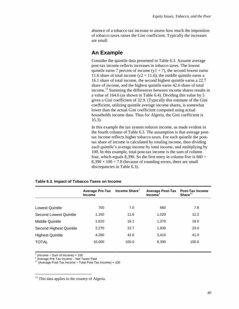
Equity Issues, Tobacco, and the Poor
40
absence of a tobacco tax increase to assess how much the imposition
of tobacco taxes raises the Gini coefficient. Typically the increases
are small.
An Example
Consider the quintile data presented in Table 6.3. Assume average
post-tax income reflects increases in tobacco taxes. The lowest
quintile earns 7 percent of income (y1 = 7), the second lowest earns
11.6 share of total income (y2 = 11.6), the middle quintile earns a
16.1 share of total income, the second highest quintile earns a 22.7
share of income, and the highest quintile earns 42.6 share of total
income.13
Summing the differences between income shares results in
a value of 164.6 (as shown in Table 6.4). Dividing this value by 5
gives a Gini coefficient of 32.9. (Typically this estimate of the Gini
coefficient, utilizing quintile average income shares, is somewhat
lower than the actual Gini coefficient computed using actual
households income data. Thus for Algeria, the Gini coefficient is
35.3).
In this example the tax system reduces income, as made evident in
the fourth column of Table 6.3. The assumption is that average post-
tax income reflects higher tobacco taxes. For each quintile the post-
tax share of income is calculated by totaling income, then dividing
each quintile’s average income by total income, and multiplying by
100. In this example, total post-tax income is the sum of column
four, which equals 8,390. So the first entry in column five is 660 ÷
8,390 × 100 = 7.8 (because of rounding errors, there are small
discrepancies in Table 6.3).
13
This data applies to the country of Algeria.
Table 6.3. Impact of Tobacco Taxes on Income
Average Pre-Tax Income
Income Share† Average Post-Tax
Income‡
Post-Tax Income Share
††
Lowest Quintile 700 7.0 660 7.8
Second Lowest Quintile 1,160 11.6 1,020 12.2
Middle Quintile 1,610 16.1 1,370 16.0
Second Highest Quintile 2,270 22.7 1,930 23.0
Highest Quintile 4,260 42.6 3,410 41.0
TOTAL 10,000 100.0 8,390 100.0
† (Income ÷ Sum of Income) × 100 ‡ Average Pre-Tax Income – Net Taxes Paid ††
(Average Post-Tax Income ÷ Total Post-Tax Income) × 100

Equity Issues, Tobacco, and the Poor
41
Using the post-tax income shares, compute income share difference
(shown in Table 6.5). Determine the Gini coefficient by dividing the
sum of the share differences (154.4) by 5 to get 30.9. Hence, the
originally estimated Gini coefficient (above) drops from 32.9 to 30.9.
The conclusion is that the tax system generates a pattern of
disposable income that is more equitable than would exist in the
absence of the tax system. Since the Gini coefficient declines, even
taking into account higher tobacco taxes, the tax system remains
progressive and increases equity. In this case, the imposition of
tobacco taxes does not lead to an increase in inequity, at least as
measured by the Gini coefficient, and concerns about the fairness of
the tobacco tax increase are less compelling.
Compute Gini Coefficients with a Spreadsheet
A Microsoft Excel spreadsheet is provided as an electronic
addendum to this Tool to compute Gini coefficients from quintile
data. Data that the investigator must supply is indicated in blue. To
fully utilize the spreadsheet, the following information for each
income quintile is required (these are quintile averages):
income
expenditure
property income
dividends
housing expenditures
non-tobacco excise tax payments
Table 6.4. Income Share Difference for Pre-Tax Income
y1 = 7.0 y2 = 11.6 y3 = 16.1 y4 = 22.7 y5 = 42.6 TOTAL
y1 = 7.0 0 (y1 – y1)
4.6 (y2 – y1)
9.1 (y3 – y1)
15.7 (y4 – y1)
35.6 (y5 – y1)
65.0
y2 = 11.6 0 (y2 – y2)
4.5 (y3 – y2)
11.1 (y4 – y2)
31.0 (y5 – y2)
46.6
y3 = 16.1 0 (y3 – y3)
6.6 (y4 – y3)
26.5 (y5 – y3)
33.1
y4 = 22.7 0 (y4 – y4)
19.9 (y5 – y4)
19.9
y5 = 42.6 0 (y5 – y5)
0
TOTAL 0.0 4.6 13.6 33.4 113.0 164.6

Equity Issues, Tobacco, and the Poor
42
sales taxes (VAT taxes)
tobacco tax payments
total corporate income taxes collected
If data is not available, there are several options. First, treat the data
as missing by assigning it a value of zero. Second, if total amounts
are available from, say, National Income and Product Account data
or the Ministry of Finance, then apportion totals according to income
shares.
There are two sets of incidence assumptions to invoke; one is a set of
progressive assumptions, and the other is a set of typically more
regressive assumptions. The incidence assumption is indicated in
red. The progressive scenario assumes that the burden of property
taxes falls on property income and that corporate taxes fall on
shareholders and property holders. The regressive scenario assumes
that corporate taxes are shifted to the consumers of corporate output
and that property taxes function as a tax on the consumption of
housing services. Both the Gini coefficients and the change in the
Gini coefficient are indicated in green.
Consider a Minimalist Approach
In the absence of detailed data about the structure of taxes and
sources of income, it is useful to undertake the following exercise.
Suppose that average income by quintile is available. For each
quintile, determine the corresponding income tax liability associated
with average quintile income. Then determine for each quintile
average tobacco taxes paid. If total excise tax payments are
available, apportion them into quintiles according to the quintile
Table 6.5. Income Share Difference for Post-Tax Income
y1 = 7.8 y2 = 12.2 y3 = 16.0 y4 = 23.0 y5 = 41.0 TOTAL
y1 = 7.0 0 (y1 – y1)
4.4 (y2 – y1)
8.2 (y3 – y1)
15.2 (y4 – y1)
33.3 (y5 – y1)
61.0
y2 = 11.6 0 (y2 – y2)
3.8 (y3 – y2)
10.8 (y4 – y2)
28.8 (y5 – y2)
43.4
y3 = 16.1 0 (y3 – y3)
7.0 (y4 – y3)
25.0 (y5 – y3)
32.0
y4 = 22.7 0 (y4 – y4)
18.0 (y5 – y4)
18.0
y5 = 42.6 0 (y5 – y5)
0
TOTAL 0.0 4.4 12.0 33.0 105.0 154.4

Equity Issues, Tobacco, and the Poor
43
share of tobacco taxes paid. Then sum the tax payments, income, and
tobacco excise taxes (and other excise taxes if available) for each
quintile and compute after tax quintile income. For the pre-tax
income and resulting post-tax income, calculate the Gini coefficients
and examine the change in Gini coefficients; if the Gini coefficient
declines for post-tax income, this provides some evidence that the
overall tax system is progressive.
Ultimately, the entire fiscal system is relevant in determining the
impact of higher tobacco taxes. This means that, in addition to taxes,
one should also consider all government expenditures and transfer
payments in determining the impact of government activity on the
distribution of income. Government expenditures on health,
education, housing, as well as direct cash transfers to low income
families must be assessed and calculated. Such government
expenditures, in conjunction with taxes, are then jointly taken into
account in determining the overall progressivity of the fiscal system.
Compute and compare the Gini coefficients, both before and after
taking into account all taxes and expenditures. If the Gini coefficient
after the impact of the entire fiscal system is taken into account
declines, then the overall fiscal system is progressive.

Equity Issues, Tobacco, and the Poor
44
VIII. Conclusion
The objection that higher taxes injure the poor is a very potent
argument against one of the prime methods of tobacco control. This
Tool identifies ways of investigating the impact of higher tobacco
excise taxes on the poor. Since the amount and quality of data, as
well as the amount of time and resources available for analysis, may
vary, a range of methodological options are suggested. Thus both
approaches that are bare bones in nature as well as methodologies
that are state of the art are proposed.
A fundamental point is that there is no reason for higher tobacco
taxes to disproportionately injure the poor, so long as policies are
well designed. For instance, higher taxes can be offset in a variety of
ways. Other taxes on commodities used by the poor can be reduced.
And tobacco tax revenue can be earmarked for expenditures that
primarily benefit the poor, such as health clinics, capital
development projects, or education.
Additionally, because of the way the poor respond to higher tobacco
taxes, the impact of higher taxes can be ameliorated. Thus, if the
poor respond by significantly reducing tobacco consumption, then
impact on the welfare of the poor may, on average, be slight, though
this depends on the magnitude of their responses.
Finally, it is important to keep in mind that the health consequences
of tobacco consumption are much more disruptive and severe for the
poor. With little access to health care and little or incomplete
knowledge about some aspects of health and medicine, mortality and
disability rates among the poor are much higher when they acquire
tobacco related illnesses.
In short, this Tool’s basic policy conclusions and suggestions are
very straightforward. Tobacco tax increases can be offset by changes
in the pattern of government expenditures or by lowering other taxes
paid by the poor. Further, it is possible that, at the aggregate level,
the impact of higher tobacco taxes on the poor may not be as severe
as is sometimes put forth. Most of the material in this Tool examines
when this second assertion is likely to be true. If it is not true, the
first policy option is always available to remedy the impact of higher
taxes.

Equity Issues, Tobacco, and the Poor
45
IX. Additional References
Becker, G., and Murphy, K, (1988), “A theory of rational addiction,” Journal of Political Economy,
96, 675–700.
Bobak, M., Jha, P., Nguyen, S., and Jarvis, M., (2000) “Poverty and smoking,” in Jha and Chaloupka
eds., Tobacco Control in Developing Countries, Oxford: Oxford University Press, pages 41–61.
Gajalakshmi, G. K., Jha, P., Ransom, K., and Nguyen, S., “Global patterns of smoking and smoking-
attributable mortality,” in Jha and Chaloupka eds., Tobacco Control in Developing Countries,
Oxford: Oxford University Press, pages 11–39.
Hu, T., (1997), “Cigarette taxation in China: Lessons from international experiences,” Tobacco
Control, 6, 136–140.
Jha, P and Chaloupka, F., (2000) eds., Tobacco Control in Developing Countries, Oxford: Oxford
University Press.
Litchfield, J., (1999), “Inequality measures and tools,” unpublished World Bank report (available at
www.worldbank.org/poverty/inequal/methods/index.htm).
Meara (1999), “Why is health related to socioeconomic status?” unpublished paper, Harvard Medical
School.
Netzer, D., (1966), Economics of the Property Tax, Brookings Institution.
Pechman, J., and Okner, B. (1974), Who Bears the Tax Burden? Brookings Institution.
Peck, R., Chaloupka, F., Jha, P., and Lightwood, J., (2000), “A welfare analysis of tobacco use,” in
Jha and Chaloupka eds., Tobacco Control in Developing Countries, Oxford: Oxford University
Press, pages 131–151.
Peto, R., Lopez, A.D., Boreham, J., Thun, M., and Heath, C.J., (1992), “Mortality from tobacco in
developed countries: Indirect estimation from national vital statistics,” Lancet, 339, 1268–1278.
Peto, R., Lopez, A.D., Boreham, J., Thun, M., and Heath, C.J., (1994), Mortality from Smoking in
Developed Countries 1950–2000: Indirect Estimates from National Vital Statistics, Oxford:
Oxford University Press.
Poterba, (1989), “Lifetime incidence and the distributional burden of excise taxes,” American
Economic Review, 79 (May), pages 325–330.
Rosen, H., (1999), Public Finance, Fifth Edition, Irwin McGraw-Hill.
Sen, A., (1982), Poverty and Famines, Oxford: Oxford University Press.

Equity Issues, Tobacco, and the Poor
46
Sullivan, M., (2000), “Taxing the ‘sins’ of the poor: Do two wrongs make a right,” State Tax Notes,
v. 1 18 (17), April 17, 2000, pages 1377–1381.
Townsend, J., Roderick, P., and Cooper, J., (1994), “Cigarette smoking by socioeconomic group, sex,
and age: Effects of price, income and health publicity,” British Medical Journal, 309, (6959),
pages 923–927.
Warner, K., (1990), “Tobacco taxation as a health policy in the third world,” American Journal of
Public Health, 80, 529–530.
World Bank Report, (1999), Curbing The Epidemic: Governments and the Economics of Tobacco
Control, World Bank Publication.