Tomlinson Harashima Precoding for Multi-Gigabit short-haul ...

Tomlinson Harashima Precoding for Multi-Gigabit

short-haul Transmission over Plastical Optical

Fibers

Laura Caballero Nadales

September 7, 2010

2

Acknowledgments

Thanks to my family and the people who has been with me in the worst moments

of my life, for you.

Institut für Nachrichtenübertragung Universität Stuttgart

3

Resumen

En este proyecto, el sistema de Precodi�cación Tomlinson-Harashima es estudi-

ado e implementado mediante un programa en Matlab con el objetivo de eliminar

la ISI en nuestro canal. Nuestro canal es característico de las POF (Plastic Optical

Fiber) y tiene ciertas características por las cuales hay que tener muy en cuenta a

la hora de aplicar el THP. El uso del THP es perfectamente justi�cable si se tienen

en cuenta las grandes ventajas que ofrece en contraposición a otras técnicas como el

DFE. El THP puede trabajar en conjunción con el Reed Solomon code para mejorar

así la BER. Más características del RS són presentadas a lo largo de la memoria

y �nalmente en la última parte, las simulaciones del THP y RS són mostradas y

posteriormente razonadas.


4

Abstract

In this dissertation, the Tomlinson-Harashima is presented and implemented by a

Matlab program with the objective to eliminate the ISI in our channel. Our channel

is characteristic by the use of Plastical Optical Fibers(POF) and the channel has

certain features that should be taken into account for the THP application. The

use of THP is justi�ed because of the great advantatges that it presents over other

techniques such as DFE, THP can works in conjuction with the Reed Solomon to

further decrease the Bit Error Ratio. More characteristics of RS are presented along

the dissertation and in the �nal part RS is combined with THP and the performance

results are shown.


Contents

1 Backgrounds of Tomlinson Harashima 9

1.1 Introduction . . . . . . . . . . . . . . . . . . . . . . . . . . . . . . . . 9

1.2 Decision-Feedback Equalization . . . . . . . . . . . . . . . . . . . . . 9

1.3 Precoding Schemes . . . . . . . . . . . . . . . . . . . . . . . . . . . . 12

1.4 Tomlinson Harashima Precoding . . . . . . . . . . . . . . . . . . . . . 13

1.4.1 History . . . . . . . . . . . . . . . . . . . . . . . . . . . . . . . 13

1.4.2 De�nition . . . . . . . . . . . . . . . . . . . . . . . . . . . . . 13

1.4.3 Mathematical concept . . . . . . . . . . . . . . . . . . . . . . 14

1.4.4 Losses of Tomlinson-Harashima Precoding . . . . . . . . . . . 19

1.4.5 THP under di�erent criterions . . . . . . . . . . . . . . . . . 20

2 System 22

2.1 Channel . . . . . . . . . . . . . . . . . . . . . . . . . . . . . . . . . . 23

2.1.1 Polymer Optical �bers . . . . . . . . . . . . . . . . . . . . . . 24

3 Simulation results for THP 27

3.1 Comparison . . . . . . . . . . . . . . . . . . . . . . . . . . . . . . . . 31

3.2 Reasons . . . . . . . . . . . . . . . . . . . . . . . . . . . . . . . . . . 31

3.2.1 Losses . . . . . . . . . . . . . . . . . . . . . . . . . . . . . . . 31

3.2.2 Channel typology . . . . . . . . . . . . . . . . . . . . . . . . . 32

4 Backgrounds Reed Solomon 35

4.1 Introduction . . . . . . . . . . . . . . . . . . . . . . . . . . . . . . . . 35

5

CONTENTS 6

4.2 Mathematical concept . . . . . . . . . . . . . . . . . . . . . . . . . . 36

4.2.1 Galois Finite Fields . . . . . . . . . . . . . . . . . . . . . . . . 38

5 Simulations results of RS 39

6 Simulations results of RS+TH 44

7 Conclusion 46

Bibliography 49

List of Figures 50

A Reed Solomon CODE 52

B Tomlinson Harashima CODE 54

C Tomlinson Harashima and Reed Solomon CODE 58


CONTENTS 7

Acronyms

BER Bit Error Ratio

DFE Decision Feedback Equalizer

EDS E�ective Data Sequence

FEC Forward Error Correction

ISI Intersymbol Interferece

MMSE Minimum Mean Square Error

MIMO Multiple Input Multiple Output

PAM Pulse Amplitud Modulation

POF Polymer Optical Fiber

RS Reed- Solomon

TH Tomlinson-Harashima

SER Symbol Error Ratio

SISO Single Input Single Output

SNR Signal-to-Noise-Ratio

ZF ZeroForcing


Chapter 1

Backgrounds of Tomlinson

Harashima

1.1 Introduction

To overcome the multipath e�ect ( ISI-Intersymbol Interference-) and achieve high

throughput transmission, channel equalization or precoding techniques can be used.

However, in linear equalization there are some limitations, for example in case of

severe ISI the performance of the linear equalizer is limited and su�ers from noise

enhancement. Thus, this dissertation will show how to improve the system per-

formance by nonlinear equalization. The most commonly used nonlinear equalizer

is the Decision-Feedback Equalizer, but it has some drawbacks, thus Tomlinson-

Harashima precoding technique is introduced in this dissertation as the main option

to overcome the drawbacks of DFE.

1.2 Decision-Feedback Equalization

The Decision Feedback Equalizer (DFE) is the improved equalizer according to the

linear equalizer by the introduced nonlinearity [1]. The DFE has a noise reduction

9

1. Backgrounds of Tomlinson Harashima 10

according to the linear equalizer which su�ers from noise enhancement.

A disadvantage of DFE is that erroneous decisions lead to residual postcursive

ISI and this can possible result in further decision errors, a phenomen known as

error propagation (EP) in its feedback loop. Error propagation is exacerbated when

DFE is combined with coded modulation techniques using dense constellations. As

the constellation distances become smaller, symbol-by-symbol decisions become less

accurate. In our case, MPAM is considered, whose constellation distances decreases

when M increases, causing a severer error propagation.

DFE is composed of two �lters: The feedforward �lter and feedback �lter. Both

are implemented at, in general, symbol rate. In the DFE, the input from the chan-

nel is passed through a feedforward �lter. The output of the feedback �lter is then

subtracted from the output of the feedforward �lter.

The block diagram of the DFE is given in Figure 1.1:

Figure 1.1: Block diagram of DFE



The feedforward �lter removes some of the ISI from the received signal, but

leaves some of the postcursor ISI on the signal (generally, all postcursor ISI). The

feedback �lter estimates the residual ISI from the past decisions and subtracts it

from the feedforward �lter output. The DFE solution is better than linear equalizer

with a low-complexity solution.

The low noise enhancement of the DFE arises from the fact that, by assuming

no decision errors, the decision device removes all the noise present in the signal

[1]. So, if the inputs of the feedback �lter have no noise then the outputs of the

feedback �lter have no noise. Also, the feedforward �lter has the less complex prob-

lem of removing only precursor coe�cients. This results in a better performance

for the feedforward �lter comparing to the linear equalizer. But, the assumption of

correct symbol decisions at the output of the decision device may not work in practi-

cal cases, so error propagation occurs and the performance of the equalizer degrades.

To cope with these problems exposed before, the precoding technique is intro-

duced.



1.3 Precoding Schemes

The original principle of precoding is that if transmitter knows the channel infor-

mation, we can design the transmit signal so that the ISI in the receiver side is

greatly mitigated. For instance, the use of Tomlinson-Harashima Precoding can be

regarded as moving the feedback �lter of DFE to the transmit side to avoid error

propagation problem.

In this section precoding techniques are discussed, by employing precoding, the

disadvantages of DFE can be avoided: Coding techniques can be applied in the same

way as for channels without ISI, and no error propagation occurs.

These techniques are always apply if known in advance by the transmitter, the

channel transfer function. Although the channel is not fully known by the trans-

mitter, the use of precoding is still correct but with a set of compromises, such as

removing the residual intersymbol interference (caused by estimation errors) through

the linear adaptive equalization in the receiver.

Basically, two precoding techniques are known: Tomlinson-Harashima precoding

(THP), which was proposed almost 30 years ago, and �exible precoding (FLP)[5],

developed recently during the standards activities for the international telephone

line modem standard ITU V.34.

In contrast to THP which is derived from linear preequalization at the trans-

mitter, �exible precoding resembles linear equalization at the receiver side. The

disadvantage of linear equalization is that the channel noise is �ltered with 1H(z)

,

too, and thus the desired prediction gain is lost.



1.4 Tomlinson Harashima Precoding

1.4.1 History

Tomlinson-Harashima precoding(THP) was invented independently and more or less

simultaneously (1968-1969) in theses by Tomlinson in the United Kingdom and Ha-

rashima in Japan. They applied THP to a SISO system without adaptive receive

�lter in order to suppress the ISI caused by the frequency selectivity of the channel,

since the recursive �lter necessary to equalize the channel can be unstable.

Later, Ginis and Fischer proposed Spatial THP without ordering for �at fading

MIMO channels. Whereas Ginis included a feedforward �lter in the transmitter

and assumed a receive �lter which is a diagonal matrix, Fischer investigated a sys-

tem with the feedforward �lter at the receiver. Further Fischer and Simeone were

the only ones to investigate the THP with partial channel state information at the

transmitter.

Finally, Joham presented the necessary optimizations for THP with FIR feed-

forward and feedback �lters for frequency selective MIMO channels and Fischer

designed THP for frequency selective MIMO channels with IIR feedforward �lter by

applying a spectral factorization of the channel transfer function.

1.4.2 De�nition

Tomlinson-Harashima precoding is a transmitter equalization technique where equal-

ization is performed at the transmitter side, and has been widely used in many ap-

plications, such as DSL systems, voice band and cable modems. It can eliminate

error propagation by moving the FBF of DFE to the transmitter and allow us to use

current capacity-achieving channel codes, such as low-density parity-check (LDPC)

codes in a natural way. Recently, TH precoding has been proposed to be used in 10

Gigabit Ethernet over copper (10 GBASE-T)[2].



1.4.3 Mathematical concept

Tomlinson-Harashima precoding was originally proposed for use with an M-point

one-dimensional PAM signal setA = ±1,±2,±3, ..± (M − 1). For this constellation

THP is almost identical to the inverse channel �lter 1H(z)

, except that an o�set-free

(symmetrical about the origin) modulo-2M adder is used instead of the conventional

adder.

Figure 1.2: Output vs Input for the modulo adder.[12]

Figure 1.2 shows an example plot of the function employed by the modulo adder

for M = 4. The modulo adder over a �xed interval of, say, [−M,+M) implements

the following algorithm:

• If the result of the summation, x(k) is greater than M, 2M is deducted from

it until it is less than M.

• If the result of the summation, x(k) is less than -M, 2M is added to it until it

is greater than or equal to -M.

The block diagram of the Tomlinson-Harashima precoder using a sawtooth non-



linearity for modulo reduction is sketched in Figure 1.3 [4].

Figure 1.3: Tomlinson-Harashima precoder and linearized description

As we see that the TH structure could be conceived in two ways. The �rst way

is: in the left part of the �gure there is a sequence a[k] that is deducted by f [k].

The f [k] is the result of �ltering the output sequence x[k] with the channel impulse

response substracted by one unit in the �rst element. At this point the result of the

addition is subjected by the explained modulo adder and, thus x[k] can be obtained.

The second manner to understand the TH structure is as follows: unique se-

quence d[k] ∈ 2MZ(considering Z as an integer number) is added to the data

sequence a[k] in order to create an e�ective data Sequence (EDS) v[k], with v[k] =

a[k] + d[k], v[k] is then �ltered with the inverse of H(z).

Below shows the mathematical relationship between the sequences:

x[k] = a[k] + d[k]−p∑

K=1

h[K] · x[k −K] = v[k]− f [k] (1.1)

The values d[k] are implicitly selected symbol-by-symbol by the memoryless mod-

ulo operation, which reduces x[k] to the interval [−M,+M) .



The principle of modulo precoding can be understood as a multiple-symbol rep-

resentation based on congruent signal levels. The congruent signal points are gen-

erated by extending the signal set A periodically to the set [4].

V ≡ A+ 2MZ = a+ d| a ∈ A, d ∈ 2MZ (1.2)

Next �gure shows the extended signal set V :

Figure 1.4: Extended signal set V with M = 4.

The THP uses the signal V set instead of A, hence THP is an extension of

linear preequalization. The current e�ective data symbol is selected in THP, which

is congruent to the current a[k] , and minimizes the magnitude of the corresponding

channel symbol x[k]. It is noteworthy that THP not only has to be matched to the

channel, but also is closely tied to the actual signal constellation A.



Next Figure 1.5 shows the complete scheme for a transmission with THP:

Figure 1.5: Complete scheme for a transmission with THP.

Following we can conclude that the receiver output sequence is given by:

r[k] = v′[k] =

p∑K=0

h[K] · x[k −K] + n[k] = x[k] +

p∑K=1

h[K] · x[k −K] + n[k] =

= x[k] + f [k] + n[k] = v[k]− f [k] + f [k] + n[k] = v[k] + n[k] (1.3)

where n[k] is again the white Gaussian noise sequence.

It can be easily deduced, that in absence of noise, v[k] can be recovered directly

before the entry of the last Mod 2M , then the output v[k] would be reduced to the



range R=[-M,M) by the modulo reductor without any ISI.

Theorical SER of THP

The probability of a correct decision of a′[k] can be written as:

Pc =1

M

∑p∈A

∞∑s=−∞

Pr {z[k] = s|a[k] = p} · Pr {a′[k] = p|a[k] = p, z[k] = s} (1.4)

where z[k] is the integer element that restrict x[k] within the interval [−M,M),

and p is a particular symbol in signal set A. Finally, s is considered as an integer

number.

The decision variable y[k] is obtained by continuously folding the sample (a[k] +

2Mz[k] + f [k] + n[k]) in the interval [−M,M). It that suggest that

Pr = {a′[k] = p|a[k] = p, z[k] = s} = Pr {p− 1 < y[k] > p+ 1|a[k] = p, z[k] = s} =∞∑

m=−∞

Pr {2(m− s)M − 1 < f [k] + n[k] ≤ 2(m− s)M + 1|a[k] = p, z[k] = s} =

∞∑m=−∞

Pr {2mM − 1 < f [k] + n[k] < 2mM + 1} (1.5)

The �nal step in the above equation is obtained by using the following facts: the

summation is made from m = −∞ to ∞ so that the integer s has no e�ect on the

resultant value and the inequality 2(m− s)M − 1 < f [k] + n[k] ≤ 2(m− s)M + 1 is

free from the condition of a[k] = p and z[k] = s.



Now substituting, it yields:

Pc =∞∑

m=−∞

Pr {2(m− s)M − 1 < f [k] + n[k] ≤ 2(m− s)M + 1}

·

[1

M

∑p∈A

∞∑s=−∞

Pr {z[k] = s|a[k] = p}

](1.6)

Note that the last term in brackets is equal to 1, then the SER of THP is:

Ps = 1− Pc = 1−∞∑

m=−∞

∫ 2mM+1

2mM−1fε(x)dx (1.7)

where m is an integer, and fε(x) is the probability density function of the dis-

turbance ε[k] = f [k] + n[k].

1.4.4 Losses of Tomlinson-Harashima Precoding

There are some losses limiting the performance of THP:

• Modulo loss:

To bind the transmission power, a modulo operation is used at the transmitter.

Due to the modulo operation at the receiver will be modulo errors because

when the noise is large this modulo may �ip signals to the wrong side of the

signal constellation and causes errors. These errors are referred to as modulo

errors.

• Shaping loss:



The output is uniform rather than Gaussian. This corresponds to a loss of

log2

(2πe12

)≈ 1.53dB at high SNR, and a loss of more than 4dB at low SNR.

• Power loss:

Compared to signaling using the data symbols a[k], Tomlinson-Harashima

precoding slightly increases average transmit power. This precoding loss is

only relevant for �small� signal sets and vanishes completely as the number M

of signal points goes to in�nity. Additionally, the number of nearest neighbor

points increases slightly due to the periodic extension of the constellation.

1.4.5 THP under di�erent criterions

The precoding processing, can be optimized to satisfy a ZF or a MMSE criterion.

This is the structure of THP based on ZF and MMSE criterion:

Figure 1.6: Communication system using THP with ZF and DFE

B(D) and F (D) correspond to the feedback and feedforward �lters of THP de-

signed to minimize either ZF or MMSE optimaly criteria. B(D) is closely related

to the feedback �lter of a DFE. F (D) must to be linear and time-invariant and



corresponds to the combination of the sampled matched �lter and feedforward �lter

in a DFE [13].

In the context of THP, zero-forcing implies forcind yk = 0 for all k. Spectral

factorization techniques satisfy this criterion by producing an allpass F (D) such

that H(D)F (D) is causal, monic and minimum phase (minimum delay). B(D) is

chosen to equal H(D)F (D) [13].

The MMSE-THP is obtained by choosing F (D) and B(D) to minimize VAR(nk+

yk) under the constraints that B(D) and H(D)F (D) are monic. As with the ZF-

THP, spectral factorization techniques provide the desired �lters, which are exactly

the values of B(D) and F (D) used in MMSE-DFE. Unlike the ZF-THP, H(D)F (D)

need not be causal or minimum phase, and F (D) need not be allpass [13].


Chapter 2

System

Our system is formed by: �rst of all a Reed Solomon encoder, the following part

consist of a modulation block (PAM modulation), then this modulated signal goes

throught a Tomlinson-Harashima Precoding block, afterwards the output's signal is

�ltered by the channel and then the demodulation and RS decodi�cation are applied.

This �gure allows the understanding of the system:

Figure 2.1: System scheme

22

2. System 23

2.1 Channel

The channel is not monic and obtained from the use of Plastic Optical Fiber in our

system, it has this mathematical expression:

h =A√2πσ· e−

(t−τ ·Lpof)2

2·σ2 (2.1)

Here, some parameters are de�ned:

σ = 0.132/B3dB-> �ber dispersion

τ = 4.97 · 10−9s/m -> group delay

Lpof = 10/15m -> POF lenght in meter

and it is represented as follows:

Figure 2.2: Channel impulse response

The most important feature of this channel is the fact that it varies little with

time, this could be relationed with the requirement of Tomlinson-Harashima Pre-


2. System 24

coding concerning always is applied if the channel is known in advance by the trans-

mitter. Hence, if the channel-impulse response is not so variable, THP is useful in

this situation because it is supposed that the channel transfer function is the �same�

all the time.

Because of this channel is directly related with Polymer Optical �bers,it would

be appropiate to introduce them in the theoretical way to get a rough idea of the

environment in which we work.

2.1.1 Polymer Optical �bers

In the last decade, in optical communication networks, Polymer optical �bers (POF)

are become of a great interest. They are based on the theory of generalized impulse

response of multimode channels. There are two types of POF depending if they

have been manufactured with step-index structure(SI-POF)(used in our system) or

gradual index(GI-POF).

The core material of a POF is known as PMMA (acrylic), and �uorinated poly-

mers are the cladding material, but since the late 1990s however, much higher-

performance POF based on per�uorinated polymers (mainly polyper�uorobutenylvinylether)

has begun to appear in the marketplace.

In large-diameter �bers, 96% of the cross section is the core that allows the trans-

mission of light. Similar to traditional glass �ber, POF transmits light (or data)

through the core of the �ber. The core size of POF is in some cases 100 times larger

than glass �ber.

Because the links, connectors, and installation of POF is inexpensive, is given the

name of the "consumer" of optical �ber. PMMA system is used in environments of


2. System 25

low-speed transmission and short distances, especially in digital home devices, home

networks, industrial networks and car networks. In contrast, the per�uorinated poly-

mer �bers are commonly used for much higher-speed data center applications such

as LAN wiring and building wiring.

In recent years, POF has begun to consider as a possible option for high-speed

home networking to the next generation of Gigabit/s. So European projects such as

POF-ALL and POF-PLUS have been initiated to further investigation on this type

of �ber.

The appearance of mPOF (microstructured POF), a type of a photonic crystal

�ber, is a great development in polymer �bers �eld.

These are some characteristics of POF in short:[10]

• PMMA and Polystyrene are used as �ber core, with refractive indices of 1.49

and 1.59 respectively.

• Generally, �ber cladding is made of silicone resin (refractive index 1.46).

• High refractive index di�erence is maintained between core and cladding.

• POF have high numerical aperture.

• Have high mechanical �exibility and low cost.

Modal dispersion

Modal dispersion is a distortion mechanism occurring in multimode �bers and other

waveguides, in which the signal is spread in time because the propagation velocity of

the optical signal is not the same for all modes. Dispersion is sometimes called chro-

matic dispersion to emphasize its wavelength-dependent nature, or group-velocity


2. System 26

dispersion (GVD) to emphasize the role of the group velocity. This modal dispersion

creates the limiting factor in POF systems, and this is usually the bandwidth of the

�ber itself.

This kind of dispersion is also considered as a type of intersymbol interference

(ISI). In the ray optics analogy, modal dispersion in a step-index optical �ber may

be compared to multipath propagation of a radio signal. Rays of light enter the

�ber with di�erent angles to the �ber axis, up to the �ber's acceptance angle. Rays

that enter with a shallower angle travel by a more direct path, and arrive sooner

than rays that enter at a steeper angle. The arrival of di�erent components of the

signal at di�erent times distorts the shape.


Chapter 3

Simulation results for THP

In this chapter, I have written a program developed in MATLAB (see Appendix B)

where the Tomlinson-Harashima Precoding is used. The aim of this program is to

eliminate the ISI in our channel, and then, to improve the general system perfor-

mance.

First of all, it is good to get an idea of the schematic structure of the program

before to show the simulation results. In the �rst lines, the channel features and

some simulation parameters are de�ned. The most featured simulation parameters

are the Rb that is the bit rate andM which corresponds to the order of modulation.

Afterwards, the channel impulse response seen in the last system chapter is de�ned.

Then we go into the main part of the program, where a bit sequence is created

and subjected to a PAM modulation. In this case the M = 8 = 23 is chosen, the

modulation is used because due to every symbol carries n bit, the required bandwidth

is reduced by a factor of 1/n and thus the noise as well. A lower noise level is required

because the many signal levels are much closer spaced. The advantages of PAM are

its �exibility and adaptability to the actual SNR. Higher the SNR is available, the

more bits per symbol can be transmitted to raise the transmission capacity.

27

3. Simulation results for THP 28

After modulation, the modulated signal crosses throught the Tomlinson-Harashima

Precoding block, and when it is recovered, the demodulation is the next step.

Next diagram represents the blocks in the THP program developed:

Figure 3.1: THP program structure

Finally the recovered sequence is compared with the initial one, and we can ob-

tain the BER (Bit error rate), depending on the SNR (Signal-to-Noise ratio).

In the Tomlinson-harashima Precoding block, in our case, it is not possible to

directly apply the theorical scheme found in the bibliography because the channel is

not monic and then the �rst element chnl(0) is not equal to 1. Only if the channel

is normalized by chnl(0), the original scheme of THP could be used.

Now, the graphs resulting from the simulation of Tomlinson-Harashima program

with di�erent bit rates are shown below:



Figure 3.2: BER performance for di�erent bit rates with THP.

As it is seen the BER performance with 3Gbit/s and in 2.5Gbit/s is worse than

in the case of 2Gbit/s. When the bit rate increases, the performance gets worser.

The next three graphs show the performance of DFE [11], they are useful to

compare with our �nal results:

Figure 3.3: BER performance of 8 PAM with DFE for 2Gbit/s[11]



Figure 3.4: BER performance of 8 PAM with DFE for 2.5Gbit/s[11]

Figure 3.5: BER performance of 8 PAM with DFE for 3Gbit/s[11]



3.1 Comparison

At �rst these results seem contradictory if we consider the theory exposed in the

preceding chapters, where for instance, the use of Tomlinson-Harashima Precoding

can be regarded as moving the feedback �lter of DFE to the transmit side to avoid

error propagation problem. Therefore, THP performance is supposed to have better

BER performance than the DFE. As it can be seen, this is not true in our case, the

DFE performance is better than THP. For example for the BER value of 10−2 the

DFE needs only 19.7dB to reach it, however with THP, 35dB of SNR is needed. In

both cases it is possible to observe one thing in common, when the bit rate increases

both techniques perform worse than in lower bit rate.

3.2 Reasons

Instead of the theorical results expected based on THP and DFE performance, there

are possible reasons why these assumptions are not true in this dissertation:

3.2.1 Losses

One of these reasons could be the di�erent types of losses seen in the Backgrounds

of THP: shaping loss, power loss and modulo loss.

In the particular case of the shaping loss, as we have explained in the Back-

grounds of THP is caused by the fact that the channel's output is uniform rather

than gaussian.

The power loss can be neglected because: since what TH changed is the transmit

signal power, so if we consider the SNR at the transmitter side, TH would cause

additional lost. However, we consider here the SNR at receiver, which means, we



generated the same SNR for both schemes(THP & DFE) at the receiver, since we

measured the received signal power, then add noise according to the SNR at receiver.

It doesn't take the transmit power into account.

In case of modulo loss, is caused by the errors that appear after the modulo

reduction which are the consequence when the noise is large. Related with these

modulo errors we could introduce the following section for justify the performance

achieved.

3.2.2 Channel typology

In order to understand why these modulo errors have importance in our BER per-

formance in the case of the THP use, we introduce a monic channel with the �rst

tap as a maximum:

chnl=[1.0000 0.3011]

Now we can get the simulation results after the use of this monic channel:

Figure 3.6: BER performance for 8 PAM with TH for new monolic channel



In fact, the performance becomes better when the �rst element of the monic

channel is maximum and of course the performance would be much better if chnl(0)

is far more bigger than the other taps.

Comparing the DFE at 2Gbit/s with the response of our THP with the monic

channel, it is possible to compare some speci�c values:

As it is seen the BER performances with both techniques are similar, but maybe

in the lower SNR the BER performance of DFE is a little better because of the losses

exposed before(see Losses in Backgrounds of THP), but from 30dB aproximately the

THP performance is better than DFE.

The reason why THP performs better with this monic channel, is related with

the fact that when the x precursors(x [k −K]) are �ltered in THP block to form

the f signal , if the samples of the channel are bigger than the �rst sample, the ISI

increases (f), and x is going to be reduced into the interval [−M,M) by the modulo

2M reduction much more times (d increases). Then, in �lter's output, despite that

y has no ISI, y is equivalent to the a but a�ected by the signal that has reduced the

x (in the �rst modulo reduction), which that corresponds to d . If this number of

reductions is high, the noise added is proportional depending on the output y and

the SNR is as follows:

SNR =E[a+ d]

E[n](3.1)

The next diagram allows to understand in a better way what is happens:



Figure 3.7: Diagram for explanation

hence, when the second modulo reduction is done after the noise addition, it

will be more errors due to the explained Modulo errors and the BER perfomance

becomes worse.

One solution for our channel(known as hpof channel) is to make a post equal-

ization(for example Zero Forzing equalization) to achieve that our channel is monic

and has the maximum sample of the channel in the �rst position, because we have

seen before the THP could work better under these conditions and this supposes an

improvement on the BER performance.


Chapter 4

Backgrounds Reed Solomon

4.1 Introduction

In this chapter the Reed Solomon encoding is introduced in the theorical way, ex-

plaining di�erent reasons why it is useful by adding it with THP to further improve

the system performance. The THP precoding removes inter-symbol interferences,

and RS codes are often used to reduce bit errors to a tolerating level.

The RS code is a nonbinary cyclic code, subtype of FEC(also called channel

coding),which is a type of digital signal processing that improves data reliability by

introducing a known structure(redundant data) into a data sequence prior to trans-

mission. Then, thanks to this structure, the receiver can detect and correct errors

without the need to ask the sender for additional data. Some of the advantages of

FEC are that back-channel is not required and the retransmission of data can often

be avoided. One of the applications of FEC is that these codes are used in data

storage systems.

RS describes a systematic way of building codes that could detect and correct

multiple random symbol errors. One of the reasons why Reed Solomon works prop-

erly against the exposure to noise is when a decoder corrects a byte, it replaces the

35

4. Backgrounds Reed Solomon 36

incorrect byte with the correct one, whether the error bit was being caused by one or

all eight bits corrupted being corrupted. This gives an RS code a tremendous burst-

noise advantage over binary codes, even allowing for the interleaving of binary codes.

In order to �ght against noise e�ectively, the noise duration has to be relatively

small percentage of the codeword. To represent that ensure this happens most of

the time, the receiver should be long average noise over a period of time, reducing

the e�ect of a freak streak of bad luck. Hence, error-correcting codes become more

e�cient (error performance improved) as the code block size increases.

As the redundancy of an RS code increases (lower code rate), its implementation

grows in complexity. Also, the bandwidth expansion must grow for any real-time

communications application. However, the bene�t of increased redundancy, just like

the bene�t of increased symbol size, is the improvement in bit-error performance.

4.2 Mathematical concept

Reed-Solomon codes are nonbinary cyclic codes with symbols made up of m-bit se-

quences, where m is any positive integer having a value greater than 2. RS (n, k)

codes on m-bit symbols exist for all n and k for which [8].

0 < k < n < 2m + 2 (4.1)

where k is the number of data symbols being encoded, and n is the total num-

ber of code symbols in the encoded block. For the most conventional RS (n, k) code,



(n, k) = (2m − 1, 2m − 1− 2t) (4.2)

where t is the symbol-error correcting capability of the code, and n − k = 2t is

the number of parity symbols. An extended RS code can be made up with n = 2m

or n = 2m + 1, but not any further.[8]

Reed-Solomon codes achieve the largest possible code minimum distance for any

linear code with the same encoder input and output block lengths. For nonbinary

codes, the distance between two codewords is de�ned (analogous to Hamming dis-

tance) as the number of symbols in which the sequences di�er. For Reed-Solomon

codes, the code minimum distance is given by [7]:

dmin = n− k + 1 (4.3)

The code is capable of correcting any combination of t or fewer errors, where t

can be expressed as:

t =

⌊dmin− 1

2

⌋=

⌊n− k

2

⌋(4.4)

where bxc means the largest integer not to exceed x. Equation 4.4 illustrates

that for the case of RS codes, correcting t symbol errors requires no more than 2t

parity symbols. The equation lends itself to the following intuitive reasoning. One

can say that the decoder has n − k redundant symbols to "spend", which is twice

the amount of correctable errors. For each error, one redundant symbol is used to



locate the error, and another redundant symbol is used to �nd its correct value.

In our particular case, we have used a RS code with the following values:

m = 8, then n = 255 and k = 223 (4.5)

with these values, the code is capable of correcting any combination of t or fewer

errors, in this case t is equal to 16. Correcting 16 symbol errors requires no more

than 32 parity symbols.

4.2.1 Galois Finite Fields

It is necessary to know the Galois �nite �elds(GF) to understand the encoding and

decoding of nonbinary codes. For any prime number, p , there exists a �nite �eld

denoted GF (p) that contains p elements. It is possible to extend GF (p) to a �eld

of pm elements, called an extension �eld of GF (p), and denoted by GF (pm), where

m is a nonzero positive integer. Symbols from the extension �eld GF (2m) are used

in the construction of Reed-Solomon (RS) codes [8].


Chapter 5

Simulations results of RS

This chapter consists of developing a RS code for use in conjunction with the

THP(see Appendix B).

There are some reasons for using this nonbinary cyclic code: as it has been ex-

plained in the last chapter, RS describes a systematic way of building codes that

could detect and correct multiple random symbol errors. Another reason is that

error performance is improved the code block size increases, making RS codes an

attractive choice whenever long block lengths are desired.

The RS programm wrote contains a modulation part after encoding the original

bit sequence, in particular PAM modulation. In the encoding part, the bit sequence

is transformed to a Galois array Message (belongs to Galois �nite �eld) and then is

converted to a Reed Solomon code word.

In the simulation, the RS(255,223) with m=8 is chosen(which is a commonly

used code for DVB). Since up to 16 symbols/bytes can be corrected, the code is

able to decrease BER from 10−4 to 10−9, where errorless transmission for digital

communication is achieved [14].

39

5. Simulations results of RS 40

Next theorical graph shows the RS performance(in Eb/No terms):

Figure 5.1: Error performances for RS codes [9].

If we observed the values and the trend of the curve, coincide with the explanation

in the last paragraph, then these results should be expected in the simulation results

from RS program.



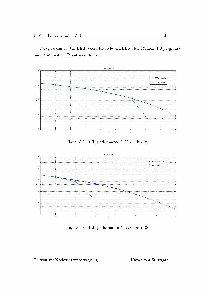
Now, we can get the BER before RS code and BER after RS from RS program's

simulation with di�erent modulations:

Figure 5.2: BER performance 2 PAM with RS





The �gures show the reduction of BER after the use of the RS code. In case of

2 PAM, the reduction occurs aproximately with 7dB of SNR, only with the increase

of 1dB till 8dB it is possible to achieve a reduction from 1.3 · 10−2 to 7 · 10−4. In 4

PAM in the range of 14-15dB, for example, the reduction is more prominent from

7 · 10−3 till 1.8 · 10−4 and �nally in 8 PAM the reduction starts with 20dB of SNR,

with SNR equal to 21dB the system can reach a value of 7 · 10−5.

In the Figures 5.1, 5.2 and 5.3 is only shown a part of the BER performance,

it is caused by the fact that the results shown above are dependent of the number

of simulations, in our case this value is 10−6, if we would want to get more values

to see that RS works as we expected, it is needed a bigger number of simulations,

but this implies a lot of time getting the results, may be we should need a computer

with higher procesing. Instead of this, we can observe the trend of the BER perfor-

mance with the use of RS prolonging it(in 8 PAM case, for example), we see that it

satis�es the theoretically expected (when the BER before RS is 10−4, BER after RS

reaches 10−9), while BER before RS needs 23.8dB(aproximately) of SNR to reach

the benchmark of 2 · 10−4, in the case of RS performance with this value of SNR,

reachs 10−9.



Now the imaginary prolongation in case of more simulations is done and repre-

sented as follows:

Figure 5.5: 8 PAM RS with prolongation.

Thus it demostrates the great use of RS, which reduces the error performance

in a substancial way for any value of modulation. An important observation is that

when M increases, a higher SNR is needed to observe the RS e�ect in the BER

performance.


Chapter 6

Simulations results of RS+TH

In this �nal chapter, the purpose is to introduce a program (see Appendix C) that

includes both RS code and THP. So in this way improvement is consist of eliminat-

ing the ISI resulting from the use of THP and reducing the error performace thanks

to the properties of RS code.

In TH program, the initial parameters and our channel are �rst de�ned. Next,

inside the main loop the original bit sequence is encoded by RS and afterwards is

modulated. The next step of this program consists of adding the THP part as it

has been created before, then the noise is added and in this point starts again the

same process described lines before but in reverse. In the �nal lines the BER after

RS and before RS are obtained to be displayed after.

The next �gure shows the BER performance achieved by the use of RS+THP

together with 8 PAM modulation, it is possible to see that in case of 2Gb/s the

BER after the use of RS+TH has a free error transmission from 37dB (with 10−6

simulations), where BER before RS decoder reaches 6·10−5. With the other bit rates

the BER achieved doesn't supposed any improvement regarding the TH program

without RS.

44

6. Simulations results of RS+TH 45

Figure 6.1: BER performance for 2Gbit/s with RS and THP.

To summarize, if we observe the results with RS+TH, the BER performance in

our system is better with the use of RS, from 10−2 this BER performance experi-

ments a great reduction comparing the BER before RS, thanks to the capacity of

detection and correction errors o�ered by RS.


Chapter 7

Conclusion

Indeed the use of TH precoding, is an improvement on the elimination of the ISI

of our channel but there are some limitations. Our channel is not monic, therefore

we have to normalize it to apply THP block in a correct way. Another point to

consider, is the fact that the rest of the channel samples have values bigger than the

initial sample, thus to reduce x we need a large number of reductions as we have seen,

a�ecting the output of channel (y). Then, in �lter's output, despite that y has no ISI,

y is equivalent to the a (modulated signal) but a�ected by the signal that has reduced

the x (in the �rst modulo reduction), which that corresponds to d . If this number

of reductions is high, the noise added is proportional depending on the output, this

causes that after the second modulo reduction will be more errors(called modulo

errors), then the BER performance becomes worser. Therefore, the application of

THP will be better if the channel is monic and the remaining samples have small

values. If it is not the case, we need to consider which could be considered as a

solution and obviously should be taken into account as future work to improve our

system, the use of an equalizer would be one of the options to be considered to

achieve the above exposed. Finally we can say that with the use of Reed Solomon

is possible to achieve a great improvement in the BER performance and it is easily

combined with THP.

46

Bibliography

[1] Edward A.Lee, David G.Messerschmitt , Digital Communication, Kluwer

Academic Publishers, Boston,1988.

[2] Yongru Gu and Keshab K. Parhi, High-Speed Architecture Design of Tom-

linson�Harashima Precoders, IEEE Transactions on circuits and systems-I: Reg-

ular Papers, Vol.54,No.9, September 2007.

[3] C. C. Jay Kuo, Shang-Ho Tsai, Layla Tadjpour and Yu-Hao Chang

Precoding Techniques for Digital Communication Systems

[4] Robert F.H.Fischer, Precoding and signal shaping for digital

transmission,Wiley-IEEE Press, New York,2002.

[5] Robert F.H.Fischer, Using �exible precoding for channels with spectral nulls,

Electronic letters,Vol.31 Issue:5,2002.

[6] Reed, Irving S. and Solomon, Gustave Polynomial Codes over Certain

Finite Fields, Journal of the Society for Industrial and Applied Mathematics.

[7] Gallager, R. G., Information Theory and Reliable Communication , New

York: John Wiley and Sons, 1968.

[8] Sklar, B., Digital Communications: Fundamentals and Applications , Second

Edition (Upper Saddle River, NJ: Prentice-Hall, 2001.

[9] Shu Lin and Daniel J. Costello Error Control Coding, 2nd ed., Pearson

Prentice Hall, NJ, 2004.

48

BIBLIOGRAPHY 49

[10] Jurgen Klauser and Olaf Ziemann Peter E.Zamzow Werner Daum

Optical Short range Transmission Systems,2nd ed.,2008,Springer

[11] Yixuan Wang Graphs Source

[12] Adnan Blind equalization for THP precoded systems

[13] Richard WeselJohn Cioffi. Achievables rates for Tomlinson-Harashima

Precoding IEEE paper

[14] Yixuan Wang Powerpoint presentation


List of Figures

1.1 Block diagram of DFE . . . . . . . . . . . . . . . . . . . . . . . . . . 10

1.2 Output vs Input for the modulo adder.[12] . . . . . . . . . . . . . . . 14

1.3 Tomlinson-Harashima precoder and linearized description . . . . . . . 15

1.4 Extended signal set V with M = 4. . . . . . . . . . . . . . . . . . . . 16

1.5 Complete scheme for a transmission with THP. . . . . . . . . . . . . 17

1.6 Communication system using THP with ZF and DFE . . . . . . . . . 20

2.1 System scheme . . . . . . . . . . . . . . . . . . . . . . . . . . . . . . 22

2.2 Channel impulse response . . . . . . . . . . . . . . . . . . . . . . . . 23

3.1 THP program structure . . . . . . . . . . . . . . . . . . . . . . . . . 28

3.2 BER performance for di�erent bit rates with THP. . . . . . . . . . . 29

3.3 BER performance of 8 PAM with DFE for 2Gbit/s[11] . . . . . . . . 29

3.4 BER performance of 8 PAM with DFE for 2.5Gbit/s[11] . . . . . . . 30

3.5 BER performance of 8 PAM with DFE for 3Gbit/s[11] . . . . . . . . 30

3.6 BER performance for 8 PAM with TH for new monolic channel . . . 32

3.7 Diagram for explanation . . . . . . . . . . . . . . . . . . . . . . . . . 34

5.1 Error performances for RS codes [9]. . . . . . . . . . . . . . . . . . . 40

5.2 BER performance 2 PAM with RS . . . . . . . . . . . . . . . . . . . 41



5.5 8 PAM RS with prolongation. . . . . . . . . . . . . . . . . . . . . . . 43

50

LIST OF FIGURES 51

6.1 BER performance for 2Gbit/s with RS and THP. . . . . . . . . . . . 45


Appendix A

Reed Solomon CODE

SNR=15:30;

BERratiobefore=ze ro s ( s i z e (SNR) ) ;

BERrat ioafter=ze ro s ( s i z e (SNR) ) ;

f o r e = 1 : l ength (SNR)

ja =0; jb=0;BERa=0;BERb=0;

whi l e jb<=10^6

m=8;k=223;M=8;n=255;

b i t s eq1 = randint (m∗k∗ l og2 (M) ,1) ;% genera t ing the sequence

ja=ja+m∗k∗ l og2 (M) ;

jb=jb+m∗n∗ l og2 (M) ;

x = reshape ( b i t seq1 ,m, k∗ l og2 (M) ) ;

xx1 = bi2de (x ' ) ;

xx2 = reshape ( xx1 , k , l og2 (M) ) ' ;

msg = g f ( xx2 ,m);%message in g a l o i s f i e l d

%encode

c = rsenc (msg , n , k ) ' ;

cc = double ( de2bi ( c . x ) ) ' ;

cc2=reshape ( cc , l og2 (M) , n∗m) ;

%modulation

h=modem.pammod( 'M' ,M, ' SymbolOrder ' , ' gray ' , ' InputType ' , ' b i t ' ) ;

y=modulate (h , cc2 ) ;

y=r e a l ( y ) ;

%no i s e added

yw=awgn(y ,SNR( e ) , ' measured ' ) ;

52

A. Reed Solomon CODE 53

h2=modem. pamdemod(h ) ;

z=demodulate (h2 , yw ) ;

z3=reshape ( z ,m∗n∗ l og2 (M) , 1 ) ;

z4=reshape ( z ,m, n∗ l og2 (M) ) ;

xx3 =bi2de ( z4 ' ) ;

xx4=reshape ( xx3 , n , l og2 (M) ) ' ;

%decode

g2=g f ( xx4 ,m) ;

q=rsdec ( g2 , n , k ) ;

H=double ( q . x ) ' ;

H2 = de2bi (H) ' ;

H3=reshape (H2 ,m∗k∗ l og2 (M) , 1 ) ;

[NUMb,RATIO]= b i t e r r ( z3 , cc ( : ) ) ;

[NUMa,RATIO2]= b i t e r r (H3 , b i t s eq1 ) ;

BERb = NUMb+BERb;

BERa = NUMa+BERa;

end

BERratiobefore ( e)=BERb/ jb ;

BERrat ioafter ( e)=BERa/ ja ;

end

d i sp ( 'BER r a t i o be f o r e RS decoder i s : ' )

d i sp ( BERratiobefore ) ;

d i sp ( 'BER r a t i o a f t e r RS decoder i s : ' )

d i sp ( BERrat ioafter ) ;

semi logy (SNR, BERratiobefore ,SNR, BERrat ioafter )

l egend ( ' BERratiobeforeRS ' , ' BERratioafterRS ' )


Appendix B

Tomlinson Harashima CODE

% POF parameters

AN = 0 . 5 ; % numerica l aper ture

Lpof = 10 ; % POF length in meter

tau = 4.97 e−3; % uni t us/m

alpha = 0 ; % f i b e r l o s s in dB/m;

A = 10^(−alpha ∗Lpof /10 ) ; % at tenuat ion over the f i b e r

AN_On = f a l s e ; % i f numerica l aper ture e f f e c t

i f AN_On

Bo=428.07/(AN^2)−1127.2/AN+1466.3; % uni t MHz

q=−0.0383/(AN^2)+0.2456/AN+0.5195;

B_3dB=Bo∗Lpof^(−q ) ; % uni t MHz

e l s e

B_3dB=1009∗Lpof ^(−0.8747); % uni t MHz

end

sigma=0.1325/B_3dB;

% Simulat ion parameters

M =8; % order o f modulation

Rb =2000; % b i t ra t e in Mbit/ s

Rs = Rb/ log2 (M) ; % symbol ra t e

f s = Rs ; % sampling f requency

NFFT = 2048 ;

t t = ( 0 :NFFT−1)/ f s ;f = f s /NFFT∗ ( 1 :NFFT−1);

% channel impulse re sponse

hpof1 = A/ sq r t (2∗ pi )/ sigma∗exp(−( tt−tau∗Lpof ) .^2/2/ sigma ^2) ;

54

B. Tomlinson Harashima CODE 55

n1 = f i nd ( abs ( hpof1)>max( hpof1 ) ∗ 0 . 0 1 ) ;chnl = hpof1 ( n1 ( 1 ) : n1 ( end ) ) ;

chnl = chnl / sq r t (sum( chnl . ^ 2 ) ) ;

f i gu r e , stem ( t t ( 1 : l ength ( chnl ) ) , chnl , ' f i l l e d ' , ' MarkerSize ' , 2 ) ;

l egend ( ' Sampled by Rs ' )

x l ab e l ( 'Time [ us ] ' )

y l ab e l ( ' hpof ( t ) ' )

g r id on

[ numfi l , numcol ]= s i z e ( n1 ) ;

chnl=chnl / chnl ( 1 ) ;

SNR=20:45;

BERratiobefore13=ze ro s ( s i z e (SNR) ) ;

SERrat iobefore13=ze ro s ( s i z e (SNR) ) ;


j =0;BERb13=0;SERb13=0;

whi l e j <=10^3

m=3000;M=8;

b i t s eq1 = randint (m∗ l og2 (M) , 1 ) ;

j=j+m∗ l og2 (M) ;

b i t s eq2 = reshape ( b i t seq1 , log2 (M) ,m) ;

%MODULATION

g=modem.pammod( 'M' ,M, ' SymbolOrder ' , ' gray ' , ' InputType ' , ' b i t ' ) ;

a=modulate ( g , b i t s eq2 ) ;

a=r e a l ( a ) ;

%TH PRECODE

x=ze ro s (1 ,m) ;

f=ze ro s (1 ,m) ;

y=ze ro s (1 ,m) ;

yn=ze ro s (1 ,m) ;

an=ze ro s (1 ,m) ;

q=ze ro s (1 ,m) ;

v=ze ro s (1 ,m) ;

b=ze ro s (1 ,m) ;

d=ze ro s (1 ,m) ;

f o r k=1:m

n=2;

i f k>=2

whi le n<=k&&n<=numcol

f ( k)= f (k)+chnl (n)∗x (k−(n−1)) ;



n=n+1;

end

end

q (k)=a (k)− f ( k ) ;

%MOD−2M

i f ( q (k)>M)

whi l e ( q (k)>M)

q (k)=q(k)−(2∗M) ;

b(k)=b(k)+(2∗M) ;

d(k)=−(b(k ) ) ;end

e l s e i f ( q ( k)<=(−M))

whi le ( q (k)<=(−M))

q (k)=q(k)+(2∗M) ;

d(k)=d(k)+(2∗M) ;

end

end

v (k)=a (k)+d(k ) ;

x ( k)=v(k)− f ( k ) ;

%FILTER

y=conv (x , chnl ) ;

%ADDING NOISE

yn (k)=awgn(y (k ) ,SNR( e ) , ' measured ' ) ;

an (k)=yn (k ) ;

%MOD 2M−a r i thmet i c

i f ( an (k)>M)

whi le ( an (k)>M)

an (k)=an (k)−(2∗M) ;

end

e l s e i f ( an (k)<=(−M))

whi le ( an (k)<=(−M))

an (k)=an (k)+(2∗M) ;

end

end

end



% DEMOD

h2=modem. pamdemod( g ) ;

z=demodulate (h2 , an ) ;

z s=modulate ( g , z ) ;

zb=reshape ( z ,m∗ l og2 (M) , 1 ) ;

[NUMs,RATIOs]=symerr ( a , z s ) ;

[NUM,RATIO]= b i t e r r ( zb , b i t s eq1 ) ;

SERb=NUMs+SERb ;

BERb=NUM+BERb;

end

BERratiobefore ( e)=BERb/ j ;

SERrat iobefore ( e)=SERb/ j ∗ l og2 (M) ;

end

f i g u r e ; semi logy (SNR, BERratiobefore ,SNR, SERrat iobefore )

legend ( ' BERratiobefore ' , ' SERrat iobefore ' )


Appendix C

Tomlinson Harashima and Reed

Solomon CODE

% POF parameters

AN = 0 . 5 ; % numerica l aper ture

Lpof = 10 ; % POF length in meter

tau = 4.97 e−3; % uni t us/m

alpha = 0 ; % f i b e r l o s s in dB/m;

A = 10^(−alpha ∗Lpof /10 ) ; % at tenuat ion over the f i b e r

AN_On = f a l s e ; % i f numerica l aper ture e f f e c t

i f AN_On

Bo=428.07/(AN^2)−1127.2/AN+1466.3; % uni t MHz

q=−0.0383/(AN^2)+0.2456/AN+0.5195;

B_3dB=Bo∗Lpof^(−q ) ; % uni t MHz

e l s e

B_3dB=1009∗Lpof ^(−0.8747); % uni t MHz

end

sigma=0.1325/B_3dB;

% Simulat ion parameters

M =8; % order o f modulation

Rb = 2000 ; % b i t ra t e in Mbit/ s

Rs = Rb/ log2 (M) ; % symbol

f s = Rs ; % sampling f requency

NFFT = 2048 ;

t t = ( 0 :NFFT−1)/ f s ;f = f s /NFFT∗ ( 1 :NFFT−1);

% channel impulse re sponse

58

C. Tomlinson Harashima and Reed Solomon CODE 59

hpof1 = A/ sq r t (2∗ pi )/ sigma∗exp(−( tt−tau∗Lpof ) .^2/2/ sigma ^2) ;

n1 = f i nd ( abs ( hpof1)>max( hpof1 ) ∗ 0 . 0 1 ) ;chnl = hpof1 ( n1 ( 1 ) : n1 ( end ) ) ;

chnl = chnl / sq r t (sum( chnl . ^ 2 ) ) ;

f i gu r e , stem ( t t ( 1 : l ength ( chnl ) ) , chnl , ' f i l l e d ' , ' MarkerSize ' , 2 ) ;

l egend ( ' Sampled by Rs ' )

x l ab e l ( 'Time [ us ] ' )

y l ab e l ( ' hpof ( t ) ' )

g r id on

[ numfi l , numcol ]= s i z e ( n1 ) ;

chnl=chnl / chnl (1);% because the channel i s not monic , i t i s nece s sa ry f o r THP apply ing

SNR=20:45;

BERratiobefore=ze ro s ( s i z e (SNR) ) ;

SERrat iobefore=ze ro s ( s i z e (SNR) ) ;

BERrat ioafter=ze ro s ( s i z e (SNR) ) ;


jb=0; j a =0;BERb=0;SERb=0;BERa=0;NUM=0;NUM2=0;NUMs=0;

whi l e jb<=10^3

m=8;k=223;M=8;n=255;

b i t s eq1 = randint (m∗k∗ l og2 (M) ,1) ;% generate seq

ja=ja+m∗k∗ l og2 (M) ;

jb=jb+m∗n∗ l og2 (M) ;

x = reshape ( b i t seq1 ,m, k∗ l og2 (M));% reo rde r the s t r u c tu r e

xx1 = bi2de (x ' ) ;% binary to decimal

xx2 = reshape ( xx1 , k , l og2 (M) ) ' ;

msg = g f ( xx2 ,m);% Message i s a Galo i s array .

%encode

c = rsenc (msg , n , k ) ' ;

cc = double ( de2bi ( c . x ) ) ' ;

cc2=reshape ( cc , l og2 (M) , n∗m) ;

%modulation

h=modem.pammod( 'M' ,M, ' SymbolOrder ' , ' gray ' , ' InputType ' , ' b i t ' ) ;

a=modulate (h , cc2 ) ;

a=r e a l ( a ) ;

%TH PRECODE

x=ze ro s (1 ,m∗n ) ;f=ze ro s (1 ,m∗n ) ;y=ze ro s (1 ,m∗n ) ;yn=ze ro s (1 ,m∗n ) ;an=ze ro s (1 ,m∗n ) ;



v=ze ro s (1 ,m∗n ) ;d=ze ro s (1 ,m∗n ) ;b=ze ro s (1 ,m∗n ) ;q=ze ro s (1 ,m∗n ) ;

f o r s =1:(m∗n)w=2;

i f s>=2

whi le w<=s&&w<=numcol

f ( s)= f ( s)+chnl (w)∗x ( s−(w−1)) ;w=w+1;

end

end

q ( s)=a ( s)− f ( s ) ;

%MOD−2Mi f ( q ( s)>=(M))

whi l e ( q ( s)>=(M))

q ( s)=q( s )−(2∗M) ;

b( s)=b( s )+(2∗M) ;

d( s)=−(b( s ) ) ;end

e l s e i f ( q ( s)<(−M))

whi le ( q ( s)<(−M))

q ( s)=q( s )+(2∗M) ;

d( s)=d( s )+(2∗M) ;

end

end

v ( s)=a ( s)+d( s ) ;

x ( s)=v( s)− f ( s ) ;

%FILTER

y=conv (x , chnl ) ;

%ADDING NOISE

yn ( s)=awgn(y ( s ) ,SNR( e ) , ' measured ' ) ; %yn ( s)=u( s)+n( s )

an ( s)=yn ( s ) ;

%MOD 2M−a r i thmet i c

i f ( an ( s)>=(M))

whi l e ( an ( s)>=(M))

an ( s)=an ( s )−(2∗M) ;

end



e l s e i f ( an ( s)<(−M))

whi le ( an ( s)<(−M))

an ( s)=an ( s )+(2∗M) ;

end

end

end

%demodulation

h2=modem. pamdemod(h ) ;

z=demodulate (h2 , an ) ;

z s=modulate (h , z ) ;

z3=reshape ( z ,m∗n∗ l og2 (M) , 1 ) ;

z4=reshape ( z ,m, n∗ l og2 (M) ) ;

xx3 =bi2de ( z4 ' ) ;

xx4=reshape ( xx3 , n , l og2 (M) ) ' ;

g2=g f ( xx4 ,m);% Message i s a Galo i s array .

%decode

q=rsdec ( g2 , n , k ) ;

H=double ( q . x ) ' ;% change type o f data

H2 = de2bi (H) ' ;

H3=reshape (H2 ,m∗k∗ l og2 (M) , 1 ) ;

[NUM,RATIO]= b i t e r r ( z3 , cc ( : ) ) ;

[NUM2,RATIO2]= b i t e r r (H3 , b i t s eq1 ) ;

[NUMs,RATIOs]=symerr ( a , z s ) ;

BERb=NUM+BERb;

BERa=NUM2+BERa;

SERb=NUMs+SERb ;

end

BERratiobefore ( e)=BERb/ jb ;

BERrat ioafter ( e)=BERa/ ja ;

SERrat iobefore ( e)=SERb/ jb ∗ l og2 (M) ;

end

d i sp ( 'BER r a t i o be f o r e RS decoder i s : ' )

d i sp ( BERratiobefore ) ;

d i sp ( 'BER r a t i o a f t e r RS decoder i s : ' )

d i sp ( BERrat ioafter ) ;

semi logy (SNR, BERratiobefore ,SNR, BERratioafter ,SNR, SERrat iobefore )



l egend ( ' BERratiobeforeRS ' , ' BERratioafterRS ' , ' SERratiobefore ' ) ;


Tomlinson Harashima Precoding for Multi-Gigabit short-haul ...

Documents

Transcript of Tomlinson Harashima Precoding for Multi-Gigabit short-haul ...