
Toll Free: 1.800.625.2488 :: Phone: 403.213.4200 :: Email ... · Analytical Solutions a) Transient...
204
Transcript of Toll Free: 1.800.625.2488 :: Phone: 403.213.4200 :: Email ... · Analytical Solutions a) Transient...

Modern Production Data Analysis
Day 1 - Theory1. Introduction to Well Performance Analysis
2. Arps – Theory
a) Exponential
b) Hyperbolic
c) Harmonic
3. Analytical Solutions
a) Transient versus Boundary Dominated
Flow
b) Boundary Dominated Flow
i. Material Balance Equation
ii. Pseudo Steady-State Concept
iii. Rate Equations
c) Transient Flow
i. Radius of Investigation Concept
ii. Transient Equation (Radial Flow)
4. Theory of Type Curves
a) Dimensionless variables
b) The log-log plot
c) Type Curve matching
5. Principle of Superposition
a) Superposition
b) Desuperposition
c) Material Balance Time
6. Gas Corrections
a) Pseudo-Pressure
b) Pseudo-Time

Modern Production Data Analysis
Day 2 - Practice7. Arps – Practical Considerations
a) Guidelines
b) Advantages
c) Limitations
8. Analysis Using Type Curves
a) Fetkovich
b) Blasingame (Integrals)
c) AG and NPI (Derivatives)
d) Transient
e) Wattenbarger
9. Flowing Material Balance
10. Specialized
11. Modeling and History Matching
12. A Systematic and Comprehensive
Approach
13. Practical Diagnostics
a) Data validation
b) Pressure support
c) Interference
d) Liquid loading
e) Accumulating skin
damage
f) Transient flow regimes
14. Tutorials
15. Selected Topics and Examples

Introduction to Well
Performance Analysis

Traditional
- Production rate only
- Using historical trends to predict future
- Empirical (curve fitting)
- Based on analogy
- Deliverables:
- Production forecast
- Recoverable Reserves under current conditions

Modern
- Rates AND Flowing Pressures
- Based on physics, not empirical
- Reservoir signal extraction and characterization
- Deliverables:
- OGIP / OOIP and Reserves
- Permeability and skin
- Drainage area and shape
- Production optimization screening
- Infill potential

Recommended Approach
- Use BOTH Traditional and Modern together
- Production Data Analysis should include a
comparison of multiple methods
- No single method always works
- Production data is varied in frequency, quality
and duration

Welltest Analysis
- High resolution
early-time
characterization
- High resolution
characterization
of the near-
wellbore
-Point-in-time
characterization
of wellbore skin
- Estimation of
reserves when
flowing pressure
is unknown
Empirical Decline
Analysis
- Flow regime
characterization over
life of well
- Estimation of fluids-
in-place
- Performance based
recovery factor
- Able to analyze
transient production
data (early-time
production, tight gas
etc)
- Characterization
of perm and skin
-Estimation of
contacted
drainage area
-Estimation of
reservoir
pressure
- Projection
of recovery
constrained
by historical
operating
conditions
Modern Production Analysis
Modern Production Analysis -
Integration of Knowledge

Arps - Empirical

Traditional Decline Curves
– J.J. Arps
- Graphical – Curve fitting exercise
- Empirical – No theoretical basis
- Implicitly assumes constant operating conditions

The Exponential Decline Curve
2001 2002 2003 2004 2005 2006
0.00
0.50
1.00
1.50
2.00
2.50
3.00
3.50
4.00
4.50
5.00
Gas R
ate,
MMscf
d
Rate vs TimeUnnamed Well
2001 2002 2003 2004 2005 2006
10-1
1.0
101
2
3
4
5
6
7
2
3
4
5
6
7
Gas R
ate
, M
Mscfd
Rate vs TimeUnnamed Well
0.00 0.10 0.20 0.30 0.40 0.50 0.60 0.70 0.80 0.90 1.00 1.10 1.20 1.30 1.40 1.50 1.60 1.70 1.80 1.90 2.00 2.10 2.20 2.30 2.40 2.50
Gas Cum. Prod., Bscf
0.00
0.50
1.00
1.50
2.00
2.50
3.00
3.50
4.00
4.50
Gas R
ate
, M
Mscfd
Rate vs. Cumulative Prod.Unnamed Well
tDi
ieqq
log log2.302
ii
D tq q
i iq q DQ
2.302*iD SlopeiD Slope
iSlope
Dq

The Hyperbolic Decline Curve
0.00 0.10 0.20 0.30 0.40 0.50 0.60 0.70 0.80 0.90 1.00 1.10 1.20 1.30 1.40 1.50 1.60 1.70 1.80 1.90 2.00 2.10 2.20 2.30 2.40 2.50 2.60
Gas Cum. Prod., Bscf
0.00
0.50
1.00
1.50
2.00
2.50
3.00
3.50
4.00
4.50
Gas R
ate
, M
Mscfd
Rate vs. Cumulative Prod.Unnamed Well
bi
i
tbD
/1)1(
( )D f t
i b
bi
DD q
q

Hyperbolic Exponent “b”
0.00 0.10 0.20 0.30 0.40 0.50 0.60 0.70 0.80 0.90 1.00 1.10 1.20 1.30 1.40 1.50 1.60 1.70 1.80 1.90 2.00 2.10 2.20 2.30 2.40 2.50 2.60
Gas Cum. Prod., Bscf
0.00
0.50
1.00
1.50
2.00
2.50
3.00
3.50
4.00
4.50
Gas R
ate,
MMsc
fd
Rate vs. Cumulative Prod.Unnamed Well
Mild Hyperbolic – b ~ 0
0.00 0.05 0.10 0.15 0.20 0.25 0.30 0.35 0.40 0.45 0.50 0.55 0.60 0.65 0.70 0.75 0.80 0.85 0.90 0.95 1.00 1.05
Gas Cumulative, Bscf
0.00
0.20
0.40
0.60
0.80
1.00
1.20
1.40
1.60
1.80
2.00
2.20
2.40
2.60
2.80
3.00
3.20
Gas
Rat
e,
MM
scfd
Rate vs. Cumulative Prod.NBU 921-22G
Strong Hyperbolic – b ~ 1

Analytical Solutions

Transient vs Boundary Dominated Flow

Transient Flow
- Early-time OR Low Permeability
- Flow that occurs while a pressure “pulse” is
moving out into an infinite or semi-infinite acting
reservoir
- Like the “fingerprint” of the reservoir
- Contains information about reservoir
properties (permeability, drainage shape)

Boundary Dominated Flow
- Late-time flow behavior
- Typically dominates long-term production data
- Reservoir is in a state of pseudo-equilibrium –
physics reduces to a mass balance
- Contains information about reservoir pore volume
(OOIP and OGIP)

Boundary Dominated Flow

Definition of Compressibility
V
pi
V
dV
pi-dp
p
V
Vc
1

Compressibility Defines Material Balance of a
Closed Oil Reservoir (above bubble point)
1 p
i
pi
t
i pss p
Nc
N p p
Np p
c N
p p m N
Note: only valid if c is constant
V=N
DV = NpDp = pi - p

Single Phase Oil MB
ip p
pN
pssmslope
ppssi Nmpp
mxy

Distance
pre
ssure
rw
Constant Rate q
1p1
Illustration of Pseudo-Steady-State
pwf1
re
2p
pwf2
2
3p
pwf3
3
time

Flowing Material Balance
pN
pssmslope
bNmpp
bmxy
ppsswfi
wfi pp
b

Steady-State Inflow Equation
Distance
pre
ssure
rw re
p
pwf
pi
Inflow (Darcy) pressure drop- Constant-
Productivity Index
),,( areaskhfb
qbpp
pss
psswf

Flowing Material Balance
Variable Rate
q
Np
pssmslope
pssppsswfi
bq
Nm
q
pp
bmxy
q
pp wfi
pssb

The Three Most Important Equations
in Modern Production Analysis
i pss pp p m N
wf pssp p qb
pssppsswfi qbNmpp

Constant Pressure
=
Production
Constant Rate
=
Welltest
q
pwf
q
pwf
Operating Conditions - Simplified

- Invert the PSS equation
1 1
( )
1
( )1
pss pi wf pss psspss
pss
pssi wf
pss
q
m Np p t m t bb
q
q b
mp p tt
b
Constant Rate Solution
Relate Back to Arps Harmonic

Constant Flowing Pressure Solution
- Required: q(t), Npmax and N for constant pwf
- Take derivative of both equations and solve for q
- Integrate to find Np(t), as t goes to infinity Np goes to Npmax
max
( )
pss
pss
mti wf b
pss
i wfp i wf t
pss
p pq t e
b
p pN p p c N
m

Constant Flowing Pressure Solution
Relate Back to Arps Exponential, Determine N
max
max
( ) ( )
i wfi
pss
pssi
pss
ip
i
t i wf t i wf i
p i
p pq
b
mD
b
qN
D
c p p c p p DN
N q

Plot Constant p and Constant q together
0
0.1
0.2
0.3
0.4
0.5
0.6
0.7
0.8
0.9
1
0 5 10 15 20 25 30 35 40 45
Constant rate q/Dp (Harmonic)
Constant pressure q/Dp (Exponential)
1
( )1
pss
pssi wf
pss
q b
mp p tt
b
( ) 1pss
pss
mt
b
i wf pss
q te
p p b

Transient Flow

-4000 -3600 -3200 -2800 -2400 -2000 -1600 -1200 -800 -400 0 400 800 1200 1600 2000 2400 2800 3200 3600 4000
Radii, ft
0
200
400
600
800
1000
1200
1400
1600
1800
2000
2200
2400
2600
2800
3000
3200
3400
3600
Pre
ssu
re,
psi
Cross Section Pressure Plot
Numerical Radial Model10
Cross Section
Plan View
Transient and Boundary Dominated Flow
Boundary Dominated
Well Performance =
f(Volume, PI)
Transient Well
Performance = f(k, skin,
time)

-4000 -3600 -3200 -2800 -2400 -2000 -1600 -1200 -800 -400 0 400 800 1200 1600 2000 2400 2800 3200 3600 4000
Radii, ft
0
200
400
600
800
1000
1200
1400
1600
1800
2000
2200
2400
2600
2800
3000
3200
3400
3600
Pre
ssu
re,
psi
Cross Section Pressure Plot
Numerical Radial Model10
Cross Section
Plan View
948
948
inv
inv
ktr
c
ktA
c
Radius (Region) of Investigation

Transient Equation
1
( ) 141.2 1 0.0063ln 0.4045
2
i wf
t
q kh
p p B kts
c
Describes radial flow in an infinite acting reservoir

q(t)’s compared
0
0.2
0.4
0.6
0.8
1
1.2
1.4
1.6
0 5 10 15 20 25 30 35 40 45
Transient flow: compares to Arps “super
hyperbolic” (b>1)

Type Curves

Blending of Transient into
Boundary Dominated Flow
0
0.5
1
1.5
2
2.5
3
0 5 10 15 20 25 30 35 40 45
Complete q(t) consists of:
Transient q(t) from t=0 to tpss
Depletion equation from t = tpss and higher

Log-Log Plot: Adds a New
Visual DynamicComparison of qD with 1/pD
Cylindrical Reservoir with Vertical Well in Center
0.000001
0.00001
0.0001
0.001
0.01
0.1
1
10
100
1000
0.000001 0.0001 0.01 1 100 10000 1000000 100000000 1E+10 1E+12 1E+14
tD
qD
an
d 1
/pD
0.9
Constant Pressure Solution Exponential
Constant Rate Solution
Harmonic
Infinite Acting Boundary Dominated

Type Curve
- Dimensionless model for reservoir / well system
- Log-log plot
- Assumes constant operating conditions
- Valuable tool for interpretation of production and
pressure data

Type Curve Example - Fetkovich
10-1 1.0 1012 3 4 5 6 7 8 9 2 3 4 5 6 7 8 2 3 4 5 6 7 8
Time
10-2
10-1
1.0
2
3
4
5
6
7
9
2
3
4
5
6
7
Rate
,Fetkovich Typecurve Analysis
Exponential
Harmonic
qDd
tDd
DdtDd eq
1
1Dd
Dd
qt
tDt
q
tqq
iDd
i
Dd
)(
Hyperbolic
1/
1
(1 )Dd
bDd
qbt

Plotting Fetkovich Type Curves-
ExampleWell 1 (exponential)
qi = 2.5 MMscfd
Di = 10 % per year
Well 2 (exponential)
qi = 10 MMscfdDi = 20 % per year
Raw Data Plot
0.00
2.00
4.00
6.00
8.00
10.00
12.00
0 5 10 15
Time (years)
Rate
(M
Mscfd
)
Well 1
Well 2
Dimensionless Plot
0.10
1.00
0.01 0.10 1.00 10.00
tDd
qD
d Well 1
Well 2
Time (years)
Well 1 Well 2 Well 1 Well 2 Well 1 Well 2
0 2.50 10.00 0.00 0.00 1.00 1.00
1 2.26 8.19 0.10 0.20 0.90 0.82
2 2.05 6.70 0.20 0.40 0.82 0.67
3 1.85 5.49 0.30 0.60 0.74 0.55
4 1.68 4.49 0.40 0.80 0.67 0.45
5 1.52 3.68 0.50 1.00 0.61 0.37
6 1.37 3.01 0.60 1.20 0.55 0.30
7 1.24 2.47 0.70 1.40 0.50 0.25
8 1.12 2.02 0.80 1.60 0.45 0.20
9 1.02 1.65 0.90 1.80 0.41 0.17
10 0.92 1.35 1.00 2.00 0.37 0.14
Rate (MMscfd) tDd qDd

Fetkovich Typecurve Matching
In most cases, we don’t know what “qi” and “Di” are ahead of time. Thus, qi and Di
are calculated based on the typecurve match (ie. The typecurve is superimposed on
the data set
t
tD
q
tqq
Ddi
Dd
i
)(
Knowing qi and Di, EUR (expected ultimate recovery) can be calculated
1.0 1013 4 5 6 7 8 9 2 3 4 5 6 7 8 9 2
Time
10-1
1.0
5
6
7
8
9
2
3
4
5
6
7
8
Rate
,
Fetkovich Typecurve AnalysisNBU 921-22G
qDd
tDd
q
t

Analytical Model Type Curve
10-4 10-3 10-2 10-1 1.0 1012 3 4 5 6 7 9 2 3 4 5 6 78 2 3 4 5 6 78 2 3 4 5 6 78 2 3 4 5 6 78 2 3 4 5 6 7
Time
10-2
10-1
1.0
101
2
3
4
6
9
2
3
4
6
9
2
3
4
6
9
2
3
4
6
Rate
,
Fetkovich Typecurve Analysis
Boundary Dominated Flow
Exponential
Transient Flow
re/rwa = 10 re/rwa = 100 re/rwa = 10,000qDd
tDd

Modeling Skin using Apparent Wellbore
Radius
rw re
rwa (s)
rwa(d)
swwa err ΔP(s)
ΔP(d)

Dimensionless Variable Definitions
(Fetkovich)
2
2
141.2 1ln
( ) 2
0.00634
1 1ln 1
2 2
eDd
i wf wa
waDd
e e
wa wa
q B rq
kh p p r
kt
ctrt
r r
r r

Type Curve Matching (Fetkovich)
2
141.2 1ln
( ) 2
0.00634 1ln
1 1ln 1
2 2
141.2 0.006342
( )
e
i wf wa Ddmatch
wwa
t Dd wae e
wa wamatch
e
i wf t Dd Dd matchmatch
B r qk
h p p r q
k t rr s
c t rr r
r r
B q tr
h p p c q t
The Fetkovich analytical typecurves can be used to calculate three parameters:
permeability, skin and reservoir radius

Type Curve Matching - Example
10-4 10-3 10-2 10-1 1.0 1012 3 4 5 6 78 2 3 4 5 6 78 2 3 4 5 6 78 2 3 4 5 6 78 2 3 4 5 6 78 2 3 4 5 6 78
Time
10-3
10-2
10-1
1.0
101
2
3
4
6
8
2
3
4
6
8
2
3
4
6
8
2
3
4
6
8
Rat
e,
Fetkovich Typecurve Analysis10
Boundary Dominated Flow
Exponential
Transient Flow
tDd
reD = 50
qDd
q
t
k = f(q/qDd)
s = f(q/qDd * t/tDd, reD)re = f(q/qDd * t/tDd)

Superposition

What about Variable Rate / Variable Pressure
Production? The Principle of Superposition
Superposition in Time:
1. Divide the production history into a series of constant rate periods
2. The observed pressure response is a result of the additive effect of each rate
change in the history
Example: Two Rate History
q1
q2
Effect of (q2-q1)
t1
1 2 1 1( ) ( ) ( )i wfp p q f t q q f t t q
pwf

The Principle of Superposition
1 2 1 1( ) ( ) ( )i wfp p q f t q q f t t
Two Rate History
N - Rate History
1 1
1
( ) ( )N
i wf j j j
j
p p q q f t t
f(t) is the Unit Step Response

Superposition versus Desuperposition
Simple
- Unit step response f(t)
- Type Curve
- Superposition Time
Complex
- Real rate and pressure
history
- Modeling (history
matching)
Superposition
Desuperposition
q
pwf
q
pwf
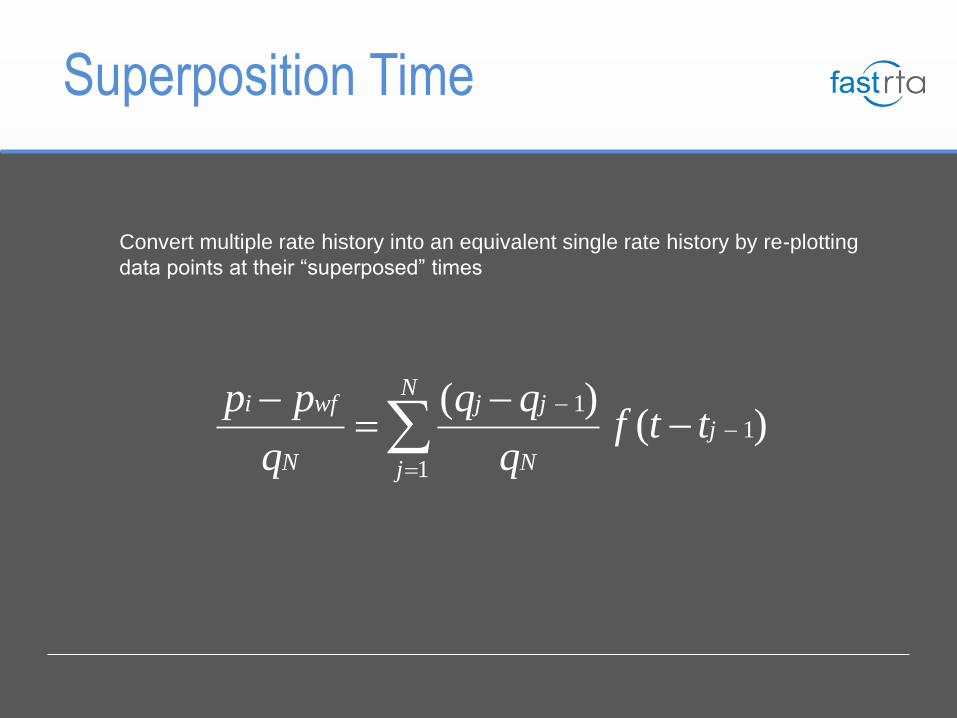
Superposition Time
Convert multiple rate history into an equivalent single rate history by re-plotting
data points at their “superposed” times
11
1
( )( )
Ni wf j j
j
N Nj
p p q qf t t
q q

The Principle of Superposition –
PSS Case
11
1
( )( )
Ni wf j j
j
N Nj
p p q qf t t
q q
141.2 3( ) ln
4
i wf e
t wa
p p t B rf t
q c N kh r
11
1
1 ( ) 141.2 3( ) ln
4
1 141.2 3ln
4
Ni wf j j e
j
N t N waj
i wf p e
N t N wa
p p q q B rt t
q c N q kh r
p p N B r
q c N q kh r
Superposition Time: Material Balance Time

Definition of Material Balance Time
(Blasingame et al)
Actual Rate Decline Equivalent Constant Rate
q
Q
actual time (t)
Q
= Q/qmaterial balance time (tc)

Features of Material Balance Time
-MBT is a superposition time function
- MBT converts VARIABLE RATE data into an
EQUIVALENT CONSTANT RATE solution.
- MBT is RIGOROUS for the BOUNDARY
DOMINATED flow regime
- MBT works very well for transient data also, but
is only an approximation (errors can be up to 20%
for linear flow)

Comparison of qD (Material Balance Time Corrected) with 1/pDCylindrical Reservoir with Vertical Well in Center
0.000001
0.00001
0.0001
0.001
0.01
0.1
1
10
100
1000
0.000001 0.0001 0.01 1 100 10000 1000000 100000000 1E+10 1E+12 1E+14
tD
qD
an
d 1
/pD
0
0.2
0.4
0.6
0.8
1
1.2
Rati
o 1
/pD
to
qD
Beginning of "semi-log" radial flow (tD=25)
Ratio (qD to 1/pD) ~ 97%
0.97
Very early time radial flow
Ratio (qD to 1/pD) ~ 90%
MBT Shifts Constant Pressure to
Equivalent Constant Rate
Constant Pressure Solution qD
Corrected to Harmonic
Constant Rate Solution
1/pD
Harmonic

Corrections for Gas Reservoirs

Corrections Required for Gas
Reservoirs
• Gas properties vary with pressure
– Formation Volume Factor
– Compressibility
– Viscosity

Corrections Required for Gas
Reservoirs
141.2 3ln
4
o ei wf
o wa
qt qB rp p
c N kh r
Depletion Term
Depends on
compressibility
Reservoir FlowTerm:
Depends on “B” and
Viscosity

Darcy’s Law Correction for Gas
Reservoirs
Darcy’s Law states : qp D
p
p
Z
pdpp
0
2
Solution: Pseudo-Pressure
For Gas Flow, this is not true because
viscosity () and Z-factor (Z) vary with pressure

Depletion Correction for Gas
Reservoirs Gas properties (compressibility and viscosity) vary
significantly with pressure
Gas Compressibility
0
0.002
0.004
0.006
0.008
0.01
0.012
0 1000 2000 3000 4000 5000 6000
Pressure (psi)
Co
mp
ressib
ilit
y (
1/p
si)
pcg
1

Solution: Pseudo-Time
g
t
g
iga
c
c
dtct
,
0
Evaluated at average reservoir
pressure
Not to be confused with welltest pseudo-time which evaluates properties
at well flowing pressure
Depletion Correction for Gas
Reservoirs: Pseudo-Time

Boundary Dominated Flow
Equation for Gas
D
4
3ln
*6417.1
)(
2
wa
ea
iig
ipwfpip
r
r
kh
Tqeqt
GZc
pppp
Pseudo-pressure Pseudo-time
Constant Rate Case
Variable Rate Case
pss
i
papb
qG
G
q
p
D
Pseudo-Cumulative Production

Overall time function - Material
Balance Pseudo-time
t
g
igta
aca
t
c
c
qdt
q
cqdt
qt
qdtq
t
00
0
1
1
0
ca
)(1
)(
t
ift
itdt
ppcc
tq
q
ct
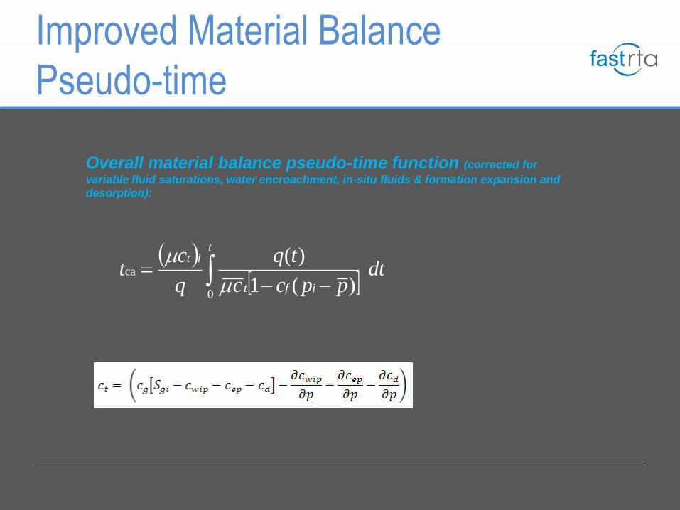
Improved Material Balance
Pseudo-time
Overall material balance pseudo-time function (corrected for
variable fluid saturations, water encroachment, in-situ fluids & formation expansion and
desorption):

Arps – Practical Consideration

Notes About Drive Mechanism and
b Value (from Arps and Fetkovich)
b value Reservoir Drive Mechanism
0 Single phase liquid expansion (oil above bubble point)
Single phase gas expansion at high pressure
Water or gas breakthrough in an oil well
0.1 - 0.4 Solution gas drive
0.4 - 0.5 Single phase gas expansion
0.5 Effective edge water drive
0.5 - 1.0 Layered reservoirs
> 1 Transient (Tight Gas)

Advantages of Traditional
- Easy and convenient
- No simplifying assumptions are required regarding the
physics of fluid flow. Thus, can be used to model very
complex systems
- Very “Real” indication of well performance

Limitations of Traditional
- Implicitly assumes constant operating conditions
- Non-unique results, especially for tight gas (transient flow)
- Provides limited information about the reservoir

Example 1: Decline Overpredicts
Reserves
October November December January February March April
2001 2002
4
Gas R
ate
, M
Mscfd
Rate vs TimeUnnamed Well
0.00 0.50 1.00 1.50 2.00 2.50 3.00 3.50 4.00 4.50 5.00 5.50 6.00 6.50 7.00 7.50 8.00 8.50 9.00 9.50 10.00 10.50
Gas Cum. Prod., Bscf
0
1
2
3
4
Gas R
ate
, M
Mscfd
Rate vs. Cumulative Prod.Unnamed Well
EUR = 9.5 bcf

Example 1 (cont’d)
Flowing Pressure and Rate vs Cumulative Production
0
0.5
1
1.5
2
2.5
3
3.5
4
4.5
5
0 1 2 3 4 5 6 7 8 9 10
Cumulative Production (bcf)
Rate
(M
Mscfd
)
0
200
400
600
800
1000
1200
Flo
win
g P
ressu
re (
psia
)
True EUR does not
exceed 4.5 bcf
Rates
Pressures
Forecast is not
valid here

Example 2: Decline Underpredicts
Reserves
0.00 0.10 0.20 0.30 0.40 0.50 0.60 0.70 0.80 0.90 1.00 1.10 1.20 1.30 1.40 1.50 1.60 1.70 1.80 1.90 2.00 2.10 2.20 2.30 2.40 2.50 2.60 2.70 2.80 2.90 3.00 3.10 3.20
Gas Cum. Prod., Bscf
0.00
0.50
1.00
1.50
2.00
2.50
3.00
3.50
4.00
4.50
5.00
5.50
6.00
6.50
7.00
7.50
8.00
8.50
Gas R
ate
, M
Mscfd
Rate vs. Cumulative Prod.Unnamed Well
EUR = 3.0 bcf

Example 2 (cont’d)
0 1 2 3 4 5 6 7 8 9 10 11 12 13 14 15 16 17 18 19 20 21 22 23 24 25
Normalized Cumulative Production, Bscf
0.000
0.005
0.010
0.015
0.020
0.025
0.030
0.035
0.040
0.045
0.050
0.055
0.060
0.065
0.070
0.075
0.080
0.085
No
rmalized
Rate
, M
Mscfd
/(10
6p
si
2/c
P)
Flowing Material BalanceUnnamed Well
Original Gas In Place
LegendDecline FMB
OGIP = 24 bcf

Example 2 (cont’d)
0 20 40 60 80 100 120 140 160 180 200 220 240 260 280 300 320 340 360 380 400 420 440 460 480 500 520 540 560 580 600 620 640 660 680 700 720
Time, days
0
1
2
3
4
5
6
7
8
9
10
11
12
13
14
15
16
17
18
Gas,
MM
scfd
0
100
200
300
400
500
600
700
800
900
1000
1100
1200
1300
Pre
ssu
re,
psi
Data ChartUnnamed Well
LegendPressure
Actual Gas Data
Operating conditions: Low drawdown
Increasing back pressure

Arps Production Forecast
0.01
0.1
1
10
Dec-00 May-06 Nov-11 May-17 Oct-22 Apr-28 Oct-33
Time
Gas R
ate
(M
Mscfd
)
Economic Limit =
0.05 MMscfd b = 0.25,
EUR = 2.0 bcf
b = 0.50,
EUR = 2.5 bcf
b = 0.80,
EUR = 3.6 bcf
Example 3 – Illustration of Non-
Uniqueness

Analysis using Type Curves

Blasingame Typecurve Analysis
Blasingame typecurves have identical format to those of Fetkovich. However, there are three important differences in presentation:
1. Models are based on constant RATE solution instead of constant pressure
2. Exponential and Hyperbolic stems are absent, only HARMONIC stem is plotted
3. Rate Integral and Rate Integral - Derivative typecurves are used (simultaneous typecurve match)
Data plotted on Blasingame typecurves makes use of MODERN DECLINE ANALYSIS methods:
- NORMALIZED RATE (q/Dp)
- MATERIAL BALANCE TIME / PSEUDO TIME

Blasingame Typecurve Analysis-
Comparison to Fetkovich
log(qDd)
log(tDd)
log(q/Dp)
log(tca)
log(qDd)
log(tDd)
log(q)
log(t)
Fetkovich Blasingame
- Usage of q/Dp and tca allow boundary dominated flow to be represented by harmonic
stem only, regardless of flowing conditions
- Blasingame harmonic stem offers an ANALYTICAL fluids-in-place solution
- Transient stems (not shown) are similar to Fetkovich

Blasingame Typecurve Analysis-
Definitions
Normalized Rate
Typecurves Data - Oil Data - Gas
D
2
1ln
2.141
wa
e
Ddr
r
Pkh
P
q
D
pP
q
D
dttqt
qDAt
Dd
DA
Ddi 0
1 D
D
ct
ci
dtP
q
tP
q
0
1 D
D
cat
pcaip
dtP
q
tP
q
0
1
DA
DdiDADdid
dt
dqtq
c
ic
id dt
P
qd
tP
q
D
D
ca
ip
ca
idp dt
P
qdt
P
q
D
D
Rate Integral
Rate Integral - Derivative

Q
rate
integral =
Q/t
actual rate
Q
actual
time
Concept of Rate Integral
(Blasingame et al)
actual
time

Rate Integral: Like a Cumulative
Average
Effective way to remove noise
t1
Average rate over time period
“0 to t1”
q
Average rate over time period
“0 to t2”
t2

D
D
ct
ci
dtp
q
tp
q
0
1
Rate Integral: Definition

Typecurve Interpretation Aids:
Integrals, Derivatives
Integral /
Cumulative
Removing the scatter from
noisy data sets
Dilutes the reservoir
signal
Fetkovich,
Blasingame, NPI
Derivative
Amplifying the reservoir
signal embedded in
production data
Amplifies noise -
often unusable
Agarwal-Gardner,
PTA
Integral-DerivativeMaximizing the strengths
of Integral and DerivativeCan still be noisy Blasingame, NPI
Used in AnalysisTypecurve Most Useful For Drawback
Other methods: Data filtering, Moving averages, Wavelet decomposition

Rate Integral and Rate Integral
Derivative (Blasingame et al)
Rate Integral
Rate (Normalized)
Rate Integral Derivative

Blasingame Typecurve Analysis-
Transient CalculationsOil:
k is obtained from rearranging the definition of
2
1
r
rln
kh
2.141
p
matchwa
eDd
D
2
1
r
rln
h
2.141
q
pq
k
matchwa
e
match
Dd
D
Solve for rwa from the definition of
2
1
r
rln1
r
rrc
2
1
kt006328.0t
matchwa
e
2
matchwa
e2
wat
cDd
2
1
matchwar
er
ln1
2
matchwar
er
2
1
tc
k006328.0
matchDdt
t
war c
wa
w
r
rlns

Blasingame Typecurve Analysis-
Boundary Dominated Calculations-OilOil-in-Place calculation is based on the harmonic stem of Fetkovich typecurves.
In Blasingame typecurve analysis, qDd and tDd are defined as follows:
ciDd
iDd tDt
pq
pqq
D
D and
/
/
Recall the Fetkovich definition for the harmonic typecurve and the PSS equation for oil in
harmonic form:
11
1
and 1
1
D
c
t
DdDd
tNbc
b
p
q
tq
From the above equations:
NbcD
bp
q
tD
p
q
p
q
t
i
i
ci
i 1 and ,
1
ere wh
1
D
D
D
PSS equation for oil in
harmonic form, using
material balance time
Definition of Harmonic
typecurve

Blasingame Typecurve Analysis-
Boundary Dominated Calculations-Oil
Oil-in-Place (N) is calculated as follows:
Rearranging the equation for Di:
bDcN
it
1
Now, substitute the definitions of qDd and tDd back into the above equation:
D
D
DdDd
c
tDd
c
Ddt
q
pq
t
t
c
pq
q
t
tc
N/1
/
1
Y-axis “match-point”
from typecurve analysis
X-axis “match-point from
typecurve analysis

bGcZ
pD
bp
q
tD
p
q
p
q
iit
ii
i
pci
i
2 and ,
1
ere wh
1
D
D
D
Blasingame Typecurve Analysis- Boundary
Dominated Calculations- GasGas-in-Place calculation is similar to that of oil, with the additional complications of pseudo-
time and pseudo-pressure.
In Blasingame typecurve analysis, qDd and tDd are defined as follows:
caiDd
ip
p
Dd tDtpq
pqq
D
D and
/
/
Recall the Fetkovich definition for the harmonic typecurve and the PSS equation for gas in
harmonic form:
1
2
1
and 1
1
D
ca
iit
ipDdDd
tbGcZ
pb
p
q
tq
PSS equation for gas in
harmonic form, using
material balance pseudo-
time
Definition of Harmonic
typecurve
From the above equations:

Gas-in-Place (Gi) is calculated as follows:
Rearranging the equation for Di:
bcZD
pG
iti
ii
2
Now, substitute the definitions of qDd and tDd back into the above equation:
Y-axis “match-point”
from typecurve analysis
X-axis “match-point from
typecurve analysis
Blasingame Typecurve Analysis-
Boundary Dominated Calculations- Gas
D
D
Dd
p
Dd
ca
it
i
p
Ddit
ca
Dd
ii
q
pq
t
t
cZ
p
pq
qcZ
t
t
pG
/2
)/(
2

Agarwal-Gardner Typecurve Analysis
Agarwal and Gardner have developed several different diagnostic
methods, each based on modern decline analysis theory. The AG
typecurves are all derived using the WELLTESTING definitions of
dimensionless rate and time (as opposed to the Fetkovich
definitions). The models are all based on the constant RATE
solution. The methods they present are as follows:
1. Rate vs. Time typecurves (tD and tDA format)
2. Cumulative Production vs. Time typecurves (tD and tDA
format)
3. Rate vs. Cumulative Production typecurves (tDA
format)
- linear format
- logarithmic format

Agarwal-Gardner Typecurve Analysis

Agarwal-Gardner - Rate vs.
Time Typecurves
Agarwal and Gardner Rate vs. Time typecurves are the same as
conventional drawdown typecurves, but are inverted and plotted in
tDA (time based on area) format.
qD vs tDA
The AG derivative plot is not a rate derivative (as per Blasingame).
Rather, it is an INVERSE PRESSURE DERIVATIVE.
pD(der) = t(dpD/dt) qD(der) = t(dqD/dt)
1/pD(der) = ( t(dpD/dt) ) -1

Agarwal-Gardner - Rate vs.
Time TypecurvesComparison to Blasingame Typecurves
Rate Integral-
Derivative
Inv. Pressure
Integral-
Derivative
qDd and tDd
plotting format
qD and tDA
plotting fomat

Agarwal-Gardner - Rate vs.
Cumulative Typecurves
Agarwal and Gardner Rate vs. Cumulative typecurves are different from
conventional typecurves because they are plotted on LINEAR
coordinates.
They are designed to analyze BOUNDARY DOMINATED data only. Thus,
they do not yield estimates of permeability and skin, only fluid-in-place.
Plot: qD (1/pD) vs QDA
Where (for oil):
tpp
tq
kh
Bq
wfi
D
2.141
wfi
i
wfit
DADDApp
pp
ppNc
QtqQ
2
1ely alternativor
)(2
1*

Where (for gas):
Agarwal-Gardner - Rate vs.
Cumulative Typecurves
t
tq
kh
Teq
wfi
D
*6417.1
wfi
i
wfiiit
caDADDA
GZc
qttqQ
2
1ely alternativor
)(
2
2
1*

Agarwal-Gardner - Rate vs.
Cumulative Typecurves
qD vs QDA typecurves
always converge to 1/2
0.159)

NPI (Normalized Pressure Integral)
NPI analysis plots a normalized PRESSURE rather than a normalized
RATE. The analysis consists of three sets of typecurves:
1. Normalized pressure vs. tc (material balance time)
2. Pressure integral vs. tc
3. Pressure integral - derivative vs. tc
- Pressure integral methodology was developed by Tom Blasingame;
originally used to interpret drawdown data with a lot of noise. (ie.
conventional pressure derivative contains far too much scatter)
- NPI utilizes a PRESSRE that is normalized using the current RATE.
It also utilizes the concepts of material balance time and pseudo-
time.

NPI (Normalized Pressure Integral):
Definitions
Normalized Pressure
Typecurves Data - Oil Data - Gas
q
PkhPD
2.141
D
q
PD
q
PpD
DA
DDd
td
dPP
ln
cdtd
q
Pd
q
P
ln
D
D
ca
p
i
p
td
q
Pd
q
P
ln
D
D
dttPt
PDAt
p
DA
Di 0
1
D
D ct
ci
dtq
P
tq
P
0
1
D
D cat
p
cai
pdt
q
P
tq
P
0
1
DA
DiDADid
dt
dPtP
c
i
c
iddt
q
Pd
tq
P
D
D
ca
i
p
ca
id
p
dt
q
Pdt
q
P
D
D
Conventional
Pressure Derivative
Pressure Integral
Pressure Integral -
Derivative

NPI (Normalized Pressure Integral):
Diagnostics
Transient
Boundary
Dominated
Integral - Derivative
Typecurve
Normalized
Pressure
Typecruve

NPI (Normalized Pressure Integral):
Calculation of Parameters- Oil
Oil - Radial
q
PkhPD
2.141
D
2
00634.0
et
c
DArC
ktt
match
D
q
P
P
hk
D
2.141
matchDA
c
t
et
t
C
kr
00634.0
matchwa
e
wq
r
re
rr
wa
w
r
rS ln
matchDA
c
match
D
t t
t
q
P
PS
CN
D
1000*615.5
2.14100634.0 0(MBBIS)

Gas – Radial
Tq
PkhP
p
D6417.1
D
2
00634.0
etii
caDA
rC
ktt
match
p
D
q
P
P
h
Tk
D
6417.1
matchDA
ca
tii
et
t
C
kr
00634.0
matchwa
e
ewa
r
r
rr
wa
w
r
rS ln
910*
6417.100634.0
match
p
D
matchDA
ca
scitii
scig
q
P
P
t
t
Pzc
TPSG
D
(bcf)
NPI (Normalized Pressure Integral):
Calculation of Parameters- Gas

Transient (tD format) Typecurves
Transient typecurves plot a normalized rate against material balance time
(similar to other methods), but use a dimensionless time based on
WELLBORE RADIUS (welltest definition of dimensionless time), rather
than AREA. The analysis consists of two sets of typecurves:
1. Normalized rate vs. tc (material balance time)
2. Inverse pressure integral - derivative vs. tc
- Transient typecurves are designed for analyzing EARLY-TIME data to
estimate PERMEABILITY and SKIN. They should not be used (on their
own) for estimating fluid-in-place
- Because of the tD format, the typecurves blend together in the early-time
and diverge during boundary dominated flow (opposite of tDA and tDd
format typecurves)

Transient versus Boundary
Scaling Formats
log(qDd)
log(tDd)log(tD)
log(qD)

Transient (tD format) Typecurves:
Definitions
Normalized Rate
Typecurves Data - Oil Data - Gas
Pkh
qqD
D
2.141
P
q
D pP
q
D
1
0
1/1
dttP
tP
DAt
p
DA
Di
1
0
1
D
Dct
ci
dtq
P
tq
PInv
1
0
1
D
Dcat
p
cai
pdt
q
P
tq
PInv
1
/1
DA
DiDADid
dt
dPtP
1
D
D
c
ic
iddt
q
Pd
tq
PInv
1
D
D
ca
i
p
ca
id
p
dt
q
Pdt
q
PInv
Inverse Pressure
Integral
Inverse Presssure
Integral - Derivative

Transient (tD format) Typecurves:
Diagnostics (Radial Model)
Transient Transition to Boundary
Dominated occurs at
different points for
different typecurves
Inverse Integral -
Derivative
Typecurve
Normalized Rate
Typecurve

Transient (tD format) Typecurves:
Finite Conductivity Fracture Model
Increasing Fracture
Conductivity (FCD
stems)
Increasing
Reservoir Size
(xe/xf stems)
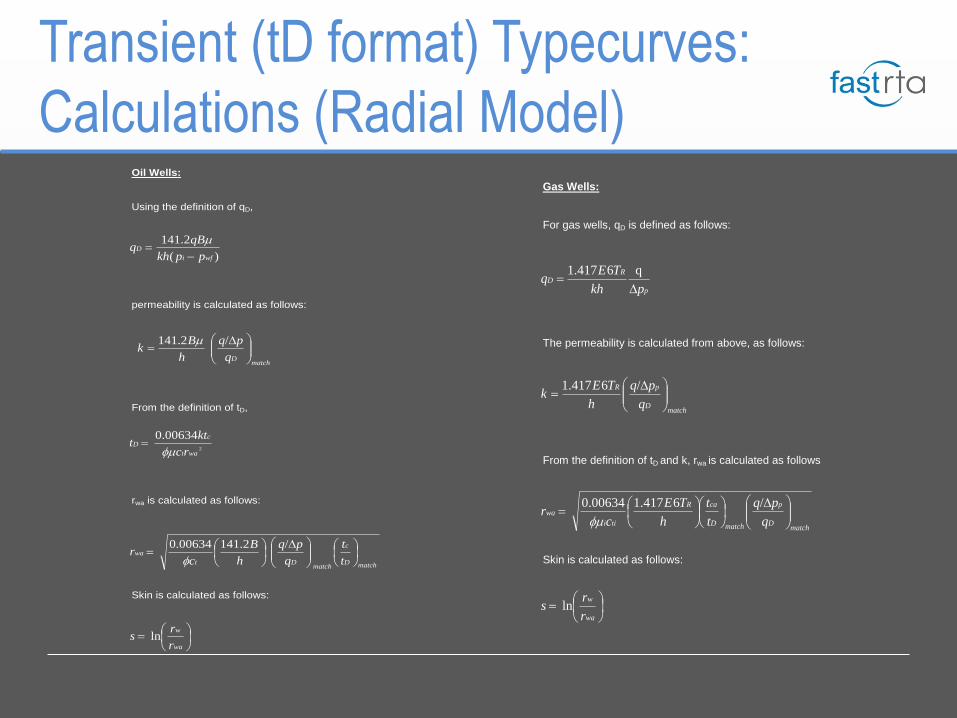
Transient (tD format) Typecurves:
Calculations (Radial Model)Oil Wells:
Using the definition of qD,
permeability is calculated as follows:
From the definition of tD,
rwa is calculated as follows:
Skin is calculated as follows:
/
2.141
matchDq
pq
h
Bk
D
/
2.14100634.0
matchD
c
matchDt
wa
t
t
q
pq
h
B
cr
D
)(
2.141
wfi
D
ppkh
qBq
00634.0
2
wat
cD
rc
ktt
ln w
war
rs
Gas Wells:
For gas wells, qD is defined as follows:
The permeability is calculated from above, as follows:
From the definition of tD and k, rwa is calculated as follows
Skin is calculated as follows:
q6.4171
p
RD
pkh
TEq
D
/6.4171
matchD
pR
q
pq
h
TEk
D
/6.417100634.0
match
D
p
matchD
caR
tii
wa
q
pq
t
t
h
TE
cr
D
ln w
war
rs

Flowing Material Balance

Flowing p/z Method for Gas –
Constant Rate
pG
Measured at well
during flow
Pressure loss due to flow
in reservoir (Darcy’s Law)
is constant with time
iG
i
i
z
p
wf
wf
z
p
- Mattar L., McNeil, R., "The 'Flowing' Gas
Material Balance", JCPT, Volume 37 #2, 1998
constant
wfz
p
z
p

pG
Measured at well
during flow
wf
wf
z
p
Graphical Method Doesn’t
Work!
Graphical Flowing p/z Method
for Gas – Variable Rate
iG ?
i
i
z
p

pG
Measured at well
during flow
Pressure loss due to flow
in reservoir is NOT
constant
iG
i
i
z
p
wf
wf
z
p
pss
wf
qbz
p
z
p
Unknown
Flowing p/z Method for Gas –
Variable Rate

Variable Rate p/z – Procedure (1)
0.00 0.10 0.20 0.30 0.40 0.50 0.60 0.70 0.80 0.90 1.00 1.10 1.20 1.30 1.40 1.50 1.60 1.70 1.80 1.90 2.00 2.10 2.20 2.30 2.40 2.50 2.60 2.70
Cumulative Production, Bscf
0
50
100
150
200
250
300
350
400
450
500
550
Flo
win
g P
ressu
re,
psi
Flowing Material BalanceUnnamed Well
Original Gas In Place
LegendStatic P/Z*
P/Z Line
Flowing Pressure
Step 1: Estimate OGIP and
plot a straight line from pi/zi
to OGIP. Include flowing
pressures (p/z)wf on plot

Variable Rate p/z – Procedure (2)
0.00 0.10 0.20 0.30 0.40 0.50 0.60 0.70 0.80 0.90 1.00 1.10 1.20 1.30 1.40 1.50 1.60 1.70 1.80 1.90 2.00 2.10 2.20 2.30 2.40 2.50 2.60 2.70
Cumulative Production, Bscf
0.00
0.40
0.80
1.20
1.60
2.00
2.40
2.80
3.20
3.60
4.00
4.40
Pro
du
cti
vit
y In
dex,
MM
scfd
/(10
6p
si
2/c
P)
0
50
100
150
200
250
300
350
400
450
500
550
Flo
win
g P
ressu
re,
psi
Flowing Material BalanceUnnamed Well
Original Gas In Place
LegendStatic P/Z*
P/Z Line
Flowing Pressure
Productivity Index
Step 2: Calculate bpss for
each production point using
the following formula:
Plot 1/bpss as a function of
Gp
line wfpss
p p
z zb
q

Variable Rate p/z – Procedure (3)
0.00 0.10 0.20 0.30 0.40 0.50 0.60 0.70 0.80 0.90 1.00 1.10 1.20 1.30 1.40 1.50 1.60 1.70 1.80 1.90 2.00 2.10 2.20 2.30 2.40 2.50 2.60 2.70
Cumulative Production, Bscf
0.00
0.40
0.80
1.20
1.60
2.00
2.40
2.80
3.20
3.60
4.00
4.40
Pro
du
cti
vit
y In
dex,
MM
scfd
/(10
6p
si
2/c
P)
0
50
100
150
200
250
300
350
400
450
500
550
Flo
win
g P
ressu
re,
psi
Flowing Material BalanceUnnamed Well
Original Gas In Place
LegendStatic P/Z*
P/Z Line
Flowing Pressure
Productivity Index
Step 3: 1/bpss should tend
towards a flat line. Iterate on
OGIP estimates until this
happens

Variable Rate p/z – Procedure (4)
0.00 0.10 0.20 0.30 0.40 0.50 0.60 0.70 0.80 0.90 1.00 1.10 1.20 1.30 1.40 1.50 1.60 1.70 1.80 1.90 2.00 2.10 2.20 2.30 2.40 2.50 2.60 2.70
Cumulative Production, Bscf
0.00
0.40
0.80
1.20
1.60
2.00
2.40
2.80
3.20
3.60
4.00
4.40
Pro
du
cti
vit
y In
dex,
MM
scfd
/(10
6p
si
2/c
P)
0
50
100
150
200
250
300
350
400
450
500
550
P/Z
*, Flo
win
g P
ressu
re,
psi
Flowing Material BalanceUnnamed Well
Original Gas In Place
LegendStatic P/Z*
P/Z Line
Flowing P/Z*
Flowing Pressure
Productivity Index
Step 4: Plot p/z points on the
p/z line using the following
formula:
“Fine tune” the OGIP estimate
pss
data wf
p pqb
z z
1/bpss

Specialized

Modeling and History Matching

Modeling and History Matching
Well / Reservoir
ModelWell Pressure at Sandface Production Volumes
Constraint (Input) Signal (Output)
Well / Reservoir
ModelProduction Volumes Well Pressure at Sandface
Constraint (Input) Signal (Output)
1. Pressure Constrained System:
2. Rate Constrained System:

Modeling and History Matching
Models - Horizontal
Rectangular reservoir with a horizontal well located anywhere inside.
L
Models - Radial
Rectangular reservoir with a vertical well located anywhere inside.
Models - Fracture
Rectangular reservoir with a vertical infinite conductivity fracture located anywhere inside.

A Systematic and Comprehensive
Method for Analysis

Modern Production Analysis
Methodology
Diagnostics Interpretation and
AnalysisModeling and
History Matching
Forecasting
- Data Chart
- Typecurves- Analytical Models
- Numerical Models
- Data Validation
- Reservoir signal
extraction
- Identifying dominant
flow regimes
- Estimating reservoir
characteristics
- Identifying important
system parameters
- Qualifying
uncertainty
- Traditional
- Fetkovich
- Blasingame
- AG / NPI
- Flowing p/z
- Transient
- Validating interpretation
- Optimizing solution
- Enabling additional
flexibility and complexity
- Reserves
- Optimization scenarios

Practical Diagnostics

• Qualitative investigation of data
– Pre-analysis, pre-modeling
– Must be quick and simple
• A VITAL component of production data
analysis (and reservoir engineering in
general)
What are diagnostics?

Illustration- Typical Dataset
0 20 40 60 80 100 120 140 160 180 200 220 240 260 280 300 320 340 360 380 400 420 440 460 480 500 520 540
Time, days
0
2
4
6
8
10
12
14
16
18
20
22
24
26
28
Liq
uid
Rate
s , b
bl/d
0.50
1.00
1.50
2.00
2.50
3.00
3.50
4.00
4.50
5.00
5.50
Gas , M
Mcfd
0
100
200
300
400
500
600
700
800
900
1000
1100
1200
1300
1400
1500
1600
Pre
ssu
re , p
si
Data ChartUnnamed Well
Legend
Pressure
Actual Gas Data

“Face Value” Analysis of Data
OGIP = 90 bcf

Go Back: Diagnostics
0 20 40 60 80 100 120 140 160 180 200 220 240 260 280 300 320 340 360 380 400 420 440 460 480 500 520 540
Time, days
0
2
4
6
8
10
12
14
16
18
20
22
24
26
28
Liq
uid
Rate
s , b
bl/d
0.50
1.00
1.50
2.00
2.50
3.00
3.50
4.00
4.50
5.00
5.50
Gas , M
Mcfd
0
100
200
300
400
500
600
700
800
900
1000
1100
1200
1300
1400
1500
1600
Pre
ssu
re , p
si
Data ChartUnnamed Well
Legend
Pressure
Actual Gas Data
Data ChartUnnamed Well
Legend
Pressure
Actual Gas Data
Pressures are not
representative of
bh deliverability

Correct Data Used
0 20 40 60 80 100 120 140 160 180 200 220 240 260 280 300 320 340 360 380 400 420 440 460 480 500 520 540
Time, days
0.00
0.50
1.00
1.50
2.00
2.50
3.00
3.50
4.00
4.50
5.00
5.50
6.00
Liq
uid
Rates , b
bl/d
0.50
1.00
1.50
2.00
2.50
3.00
3.50
4.00
4.50
5.00
5.50
Gas , M
Mcfd
4600
4800
5000
5200
5400
5600
5800
6000
6200
6400
6600
6800
7000
7200
7400
Pressu
re , p
si
Data ChartUnnamed Well
Legend
Pressure
Actual Gas Data
Oil Production
Water Production
OGIP = 19 bcf

Diagnostics using Typecurves
10-1 1.0 101 102 103 104 105 106 1074 56 8 2 3 4 5 7 9 2 3 4 5 7 9 2 3 4 56 8 2 3 4 56 8 2 3 4 56 8 2 3 4 56 8 2 3 4 56 8 2 3 4 5 7 2 3 4 5 7
10-11
10-10
10-9
10-8
10-7
2
3
5
8
2
3
5
8
2
3
5
8
2
3
5
8
2
3
5
8
2
Blasingame Typecurve Match
Radial Model
qDd
tDd
Base Model:- Vertical Well in Center of Circle
- Homogeneous, Single Layer
Transient
(concave up) Boundary Dominated
(concave down)

Material Balance DiagnosticsDiagnostics using Typecurves
10-1 1.0 101 102 103 104 105 106 1074 56 8 2 3 4 5 7 9 2 3 4 5 7 9 2 3 4 56 8 2 3 4 56 8 2 3 4 56 8 2 3 4 56 8 2 3 4 56 8 2 3 4 5 7 2 3 4 5 7
10-11
10-10
10-9
10-8
10-7
2
3
5
8
2
3
5
8
2
3
5
8
2
3
5
8
2
3
5
8
2
Blasingame Typecurve Match
Radial Model
Leaky Reservoir
(interference)
Reservoir With
Pressure Support
qDd
tDd

Productivity Diagnostics
Diagnostics using Typecurves
10-1 1.0 101 102 103 104 105 106 1074 56 8 2 3 4 5 7 9 2 3 4 5 7 9 2 3 4 56 8 2 3 4 56 8 2 3 4 56 8 2 3 4 56 8 2 3 4 56 8 2 3 4 5 7 2 3 4 5 7
10-11
10-10
10-9
10-8
10-7
2
3
5
8
2
3
5
8
2
3
5
8
2
3
5
8
2
3
5
8
2
Blasingame Typecurve Match
Radial Model
Well Cleaning Up
Liquid Loading
Increasing Damage (difficult to identify)
qDd
tDd
Productivity Shifts
(workover,
unreported tubing
change)

Transient Flow Diagnostics
Diagnostics using Typecurves
10-1 1.0 101 102 103 104 105 106 1074 56 8 2 3 4 5 7 9 2 3 4 5 7 9 2 3 4 56 8 2 3 4 56 8 2 3 4 56 8 2 3 4 56 8 2 3 4 56 8 2 3 4 5 7 2 3 4 5 7
10-11
10-10
10-9
10-8
10-7
2
3
5
8
2
3
5
8
2
3
5
8
2
3
5
8
2
3
5
8
2
Blasingame Typecurve Match
Radial Model
Transitionally
Dominated Flow (eg:
Channel or Naturally
Fractured)
Fracture Linear Flow
(Stimulated)
Radial Flow
DamagedqDd
tDd

10-1 1.0 101 102 103 104 105 106 1074 56 8 2 3 4 5 7 9 2 3 4 5 7 9 2 3 4 56 8 2 3 4 56 8 2 3 4 56 8 2 3 4 56 8 2 3 4 56 8 2 3 4 5 7 2 3 4 5 7
10-11
10-10
10-9
10-8
10-7
2
3
5
8
2
3
5
8
2
3
5
8
2
3
5
8
2
3
5
8
2
Blasingame Typecurve Match
Radial Model
Dp in reservoir is too high-Tubing size too large ?
- Initial pressure too high ?
- Wellbore correlations
underestimate pressure loss ?
Dp in reservoir is too low-Tubing size too small ?
- Initial pressure too low ?
- Wellbore correlations
overestimate pressure loss ?
qDd
tDd
“Bad Data” Diagnostics
Diagnostics using Typecurves

Selected Topics and Examples

Tight Gas

Industry Migration to Tight Gas
Reservoirs

Production Analysis – Tight Gas versus
Conventional Gas
Analysis methods are no different from that of high permeability reservoirs
Transient effects tend to be more dominant – Establishing the region (volume) of influence is critical
Drainage shape becomes more important (Transitional effects)
Linear flow is more common
Layer effects are more common

Tight Gas- Common Geometries
Tight Gas Type Curves
1.00E-11
1.00E-10
1.00E-09
1.00E-08
1.00E-07
1.00E-06
1.00E-05
1.00E-05 1.00E-04 1.00E-03 1.00E-02 1.00E-01 1.00E+00 1.00E+01 1.00E+02 1.00E+03 1.00E+04
tDd
qD
d
Linear flow
dominated Limited, bounded
drainage area
Infinite acting reservoir
1/2
1

Tight Gas Model 1
Extensive, continuous porous media; very low
permeability
Pi = 2000 psi
1800 psi
Pi = 1500 psi

Tight Gas Type Curves
1.00E-11
1.00E-10
1.00E-09
1.00E-08
1.00E-07
1.00E-06
1.00E-05
1.00E-05 1.00E-04 1.00E-03 1.00E-02 1.00E-01 1.00E+00 1.00E+01 1.00E+02 1.00E+03 1.00E+04
tDd
qD
d
1/2
Infinite Acting System

Example#1 – Infinite Acting System
10-5 10-4 10-3 10-2 10-1 1.0 101 1022 3 4 5 6 7 8 2 3 4 5 6 78 2 3 4 5 6 7 8 2 3 4 5 6 7 8 2 3 4 5 6 7 8 2 3 4 5 6 7 8 2 3 4 5 6 7 8
Material Balance Pseudo Time
10-2
10-1
1.0
101
102
2
3
5
7
2
3
5
7
2
3
4
6
9
2
3
5
7
2
3
4
6
2
No
rmalized
R
ate
Agarwal Gardner Rate vs Time Typecurve Analysis10
10-5 10-4 10-3 10-2 10-1 1.0 101 1022 3 4 5 6 7 8 2 3 4 5 6 78 2 3 4 5 6 7 8 2 3 4 5 6 7 8 2 3 4 5 6 7 8 2 3 4 5 6 7 8 2 3 4 5 6 7 8
Material Balance Pseudo Time
10-2
10-1
1.0
101
102
2
3
5
7
2
3
5
7
2
3
4
6
9
2
3
5
7
2
3
4
6
2
No
rmalized
R
ate
Agarwal Gardner Rate vs Time Typecurve Analysis10
k = 0.08 md
xf = 53 ft
OGIP = 10 bcf
k = 0.08 md
xf = 53 ft
Minimum OGIP = 2.6 bcf

No flow continuity across reservoir- Well only
drains a limited bounded volume
Tight Gas Model 2
Example: Lenticular Sands

Bounded Reservoir
Tight Gas Type Curves
1.00E-11
1.00E-10
1.00E-09
1.00E-08
1.00E-07
1.00E-06
1.00E-05
1.00E-05 1.00E-04 1.00E-03 1.00E-02 1.00E-01 1.00E+00 1.00E+01 1.00E+02 1.00E+03 1.00E+04
tDd
qD
d
1/2
1- Limited or no flow continuity in reservoir
- Very small drainage areas
- Very large effective fracture lengths
Commonly observed in practice

Example #2- Bounded Drainage
Areas
0
5
10
15
20
25
30
35
10 20 30 40 50 60 70 80 90 100 More
Drainage Area (acres)
Fre
qu
en
cy .
0%
20%
40%
60%
80%
100%
120%
Frequency Cumulative %
10-3 10-2 10-1 1.0 101 1022 3 4 5 6 78 2 3 4 5 6 78 2 3 4 5 6 78 2 3 4 5 6 78 2 3 4 5 6 78
Material Balance Pseudo Time
10-2
10-1
1.0
101
2
3
5
7
2
3
5
7
2
3
5
7
2
No
rmal
ized
Rat
e
Blasingame Typecurve AnalysisROBINSON 11-1 ALT
0
1
2
3
4
5
6
7
8
9
10
0 100 200 300 400 500 600
xf (feet)
OG
IP (
bc
f)
.
- West Louisiana gas field
- 80 acre average spacing
- All wells in boundary dominated flow

Linear flow dominated system
Tight Gas Model 3
kx
ky
Example: Naturally fractured, tight reservoir

Infinite Systems versus Linear Flow
Systems
Establish
permeability and
xf independently
Establish xf sqrt
(k) product only

Linear Flow Systems
Tight Gas Type Curves
1.00E-11
1.00E-10
1.00E-09
1.00E-08
1.00E-07
1.00E-06
1.00E-05
1.00E-05 1.00E-04 1.00E-03 1.00E-02 1.00E-01 1.00E+00 1.00E+01 1.00E+02 1.00E+03 1.00E+04
tDd
qD
d
1/2
- Channel and faulted reservoirs
- Naturally fractured (anisotropic) reservoirs
- Very large effective fracture lengths
- Very difficult to uniquely interpret
Commonly observed in practice

Example #3- Linear Flow System
101 102 1032 3 4 5 6 7 8 9 2 3 4 5 6 7 8 9 2 3 4 5 6 7 8
10-8
10-7
5
7
9
2
3
4
5
7
2
3
4
5
Blasingame Typecurve Match
Fracture Model
k = 1.1 md
xf = 511 ft
ye = 5,500 ft
yw = 2,900 ft
ye
2xf
yw

More Examples

Example #3- Multiple Layers
10-1 1.03 4 5 6 7 8 9 2 3 4 5 6 7 8 9 2 3 4 5 6 7 8 9
Material Balance Pseudo Time
10-1
1.0
9
2
3
4
5
6
7
8
2
3
No
rmalized
R
ate
Blasingame Typecurve Analysis
1.0 101 102 103 1042 3 4 5 6 7 8 9 2 3 4 5 6 7 8 9 2 3 4 5 6 7 8 9 2 3 4 5 6 7 8
10-10
10-9
10-8
2
3
4
6
8
2
3
4
5
7
Blasingame Typecurve Match
Multi Layer ModelWell
- Blasingame typecurve match, using Fracture Model
- Pressure support indicated
- Three-Layer Model (one layer with very low
permeability) used, late-time match improved

Example #4- Shale Gas
10-3 10-2 10-1 1.06 7 8 9 2 3 4 5 6 7 8 9 2 3 4 5 6 7 8 9 2 3 4 5 6 7 8 9
Material Balance Pseudo Time
10-1
1.0
3
4
5
6
7
9
2
3
4
5
6
7
2
3
4
5
No
rmalized
R
ate
Agarwal Gardner Rate vs Time Typecurve AnalysisWell
- Multi-stage fractures, horizontal well
- Analyzed as a vertical well in a circle
k = 0.02 md
s = -4
OGIP = 4.5 bcf

Tight Gas: Assessing Reserve Potential
– Recovery Plots
Objectives
Determine incremental reserves that are added as the
ROI expands into the reservoir (only relevant for
infinite or semi-infinite systems)
To establish a practical range of Expected Ultimate
Recovery

Typical Recovery Profile
Recovery Curves for k = 1 md
0
1
2
3
4
5
6
7
8
9
10
0 1 2 3 4 5 6 7 8 9 10
Original Gas in Place (bcf)
EU
R (
bcf)
1 md reservoir, unfractured
(~10 bcf / section)
100% Recovery

Typical Recovery Profile
Recovery Curves for k = 1 md
0
1
2
3
4
5
6
7
8
9
10
0 1 2 3 4 5 6 7 8 9 10
Original Gas in Place (bcf)
EU
R (
bcf
)
EUR- unlimited time
Actual EUR (qab = 0.05 MMscfd)
100% Recovery
1 md reservoir, unfractured
(~10 bcf / section)

Typical Recovery Profile
Recovery Curves for k = 1 md
0
1
2
3
4
5
6
7
8
9
10
0 1 2 3 4 5 6 7 8 9 10
Original Gas in Place (bcf)
EU
R (
bcf)
EUR- 30 year EUR- unlimited time
30 Year Limited
Actual EUR (qab = 0.05 MMscfd)
100% Recovery
1 md reservoir, unfractured
(~10 bcf / section)

Typical Recovery Profile
Recovery Curves for k = 1 md
0
1
2
3
4
5
6
7
8
9
10
0 1 2 3 4 5 6 7 8 9 10
Original Gas in Place (bcf)
EU
R (
bcf)
EUR- 30 year EUR- 20 year EUR- unlimited time
20 Year Limited
30 Year Limited
Actual EUR (qab = 0.05 MMscfd)
100% Recovery
1 md reservoir, unfractured
(~10 bcf / section)

Tight Gas Recovery Profile
Recovery Curves for k = 0.02 md
0
1
2
3
4
5
6
7
8
9
10
0 1 2 3 4 5 6 7 8 9 10
Original Gas in Place (bcf)
EU
R (
bcf)
EUR- unlimited time
0.02 md reservoir,
fractured
(~10 bcf / section)
Actual EUR (qab = 0.05 MMscfd)

Tight Gas Recovery Profile
Recovery Curves for k = 0.02 md
0
1
2
3
4
5
6
7
8
9
10
0 1 2 3 4 5 6 7 8 9 10
Original Gas in Place (bcf)
EU
R (
bcf)
EUR- 30 year EUR- unlimited time
30 Year
Actual EUR (qab = 0.05 MMscfd)
0.02 md reservoir,
fractured
(~10 bcf / section)

Tight Gas Recovery Profile
Recovery Curves for k = 0.02 md
0
1
2
3
4
5
6
7
8
9
10
0 1 2 3 4 5 6 7 8 9 10
Original Gas in Place (bcf)
EU
R (
bcf)
EUR- 30 year EUR- 20 year EUR- unlimited time
30 Year20 Year
Actual EUR (qab = 0.05 MMscfd)
0.02 md reservoir, fractured
(~10 bcf / section)

Tight Gas Recovery Profile
Recovery Curves for k = 0.02 md
0
1
2
3
4
5
6
7
8
9
10
0 1 2 3 4 5 6 7 8 9 10
Original Gas in Place (bcf)
EU
R (
bcf)
EUR- 30 year EUR- 20 year EUR- unlimited time
30 Year
Max EUR (30 y) = 2 bcf
Actual EUR (qab = 0.05 MMscfd)
20 Year
0.02 md reservoir,
fractured
(~10 bcf / section)

Example – South Texas, Deep
Gas Well
1.0 101 102 1032 3 4 5 6 7 8 9 2 3 4 5 6 7 8 9 2 3 4 5 6 7 8 9 2 3 4 5 6 7 8
10-9
10-8
7
9
2
3
4
5
7
2
3
AG Typecurve Match
Fracture Model
Sqrt k X xf = 155
Min OGIP = 4.2 bcf

Example – South Texas, Deep
Gas WellRecovery Plot - Linear System
0
1
2
3
4
5
6
7
0 100 200 300 400 500 600
ROI (acres)
EU
R (
bcf)
Minimum EUR = 3.5 bcf
Maximum EUR = 6.7 bcf
Recovery period = 30 years
sqrt k X xf = 155
pi = 6971 psia

Water Drive Models

Water Drive (Aquifer) Models:
Models for reservoirs under the influence of active water encroachment can
be categorized as follows:
1. Steady State Models (inaccurate for finite reservoir sizes)
- Schilthuis
2. Pseudo Steady-State Models (geometry independent,
time discretized)
- Fetkovich
3. Single Phase Transient Models (geometry dependent)
- infinite aquifer (linear, radial or layer geometry)
- finite aquifer (linear, radial or layer geometry)
4. Modified Transient Models
- Moving saturation front approximations
- Two phase flow approximations

Water Drive (Aquifer) Models:
Pseudo Steady-State Models
PSS models (such as that of Fetkovich) use a TRANSFER
COEFFICIENT (similar to a well productivity index) to describe the
PSS rate of water influx into the reservoir, in conjunction with a
MATERIAL BALANCE model that predicts the decline in reservoir
boundary pressure over time.
The Fetkovich model is generally used to determine reservoir fluid-
in-place by history matching the CUMULATIVE PRODUCTION and
AVERAGE RESERVOIR PRESSURE.

Water Drive (Aquifer) Models:
Pseudo Steady-State Models
Advantages:
- Geometry independent (applicable to aquifers of any shape, size or
connectivity to the reservoir)
- Works well for finite sized aquifers of medium to high mobility
- Computationally efficient
Disadvantages:
- Does not provide a full time solution (transient effects are ignored)
- Does not work well for infinite acting or very low mobility aquifers

Water Drive (Aquifer) Models:
Pseudo Steady-State Model- EquationsThe Fetkovich water influx equation for a finite aquifer is:
The above equation applies to the water influx due to a constant pressure difference between aquifer and
reservoir. In practice, the reservoir pressure “p” will be declining with time. Thus, the equation must be
discretized as follows:
/
1
ieii
i
eie
WtJpe-pp
p
WW Initial encroachable water
Aquifer transfer coefficient
Reservoir boundary pressure
/
1 1
D
i
nn
ei
na
i
eie
WtJpep-p
p
WW
The average aquifer pressure at the previous timestep (n-1) is evaluated explicitly, as follows:
1
1
1
1
D
ei
n
j
ej
ia
W
W
ppn
(1)

Water Drive (Aquifer) Models:
Pseudo Steady-State Model- Equations
But there is another equation that relates the average reservoir pressure to the amount of water
influx: the material balance equation for a gas reservoir under water drive.
1 1
-1
i
ie
i
p
i
i
G
BW
G
G
z
p
z
p
Now, we have one equation with two unknowns (water influx “We” and reservoir boundary
pressure “p”)
As with the water influx equation, the material balance equation can be discretized in time:
(2) 1 1
-1
i
ie
i
p
i
i
n G
BW
G
G
z
p
z
pnn
Equations 1 and 2 are now solved simultaneously at each timestep, to obtain a discretized
reservoir pressure and water influx profile through time.
Cumulative Production
FVF at initial conditions
Gas-in-place

Water Drive (Aquifer) Models:
Transient ModelsTransient models use the full solution to the hydraulic DIFFUSIVITY EQUATION to model rates and pressures.
The transient equations can be used to model either FINITE or INFINITE acting aquifers. There are a number of different transient models available for analyzing a reservoir under active water drive:
- Radial Composite (edge water drive)- Linear (edge water drive)- Layered (bottom water drive)
Advantages:
- Offers full continuous pressure solution in the reservoir- Includes early time effects
Disadvantages:
- Geometry dependent (only a disadvantage if aquifer properties are unknown)- Limited to assumption of single phase flow - Does not account for water influx

Water Drive (Aquifer) Typecurves:
Radial Composite Model
Blasingame, AG and NPI dimensionless formats can be used to plot
typecurves for SINGLE PHASE production (oil or gas) from a reservoir under
the influence of an EDGE WATER DRIVE. A typecurve match using this
model can be used to predict
1. Reservoir fluid-in-place
2. Aquifer mobility
- These typecurves are designed to estimate fluid-in-place by
detecting the shift in fluid mobility as the transient passes the reservoir
boundaries, into the aquifer.
- Their usefulness is limited to single phase flow (ie: the transition from
reservoir fluid to aquifer is assumed to be abrupt)

Water Drive (Aquifer) Typecurves:
Definitions
Model Type: Radial Composite (two zones);
outer zone is of infinite extent
Reservoir Aquifer
aq
res
res
aq
res
aq
k
k
M
MM
Mobility Ratio (M):

Water Drive (Aquifer) Typecurves:
Diagnostics
Increasing Aquifer Mobility
(M)
M=0 (Volumetric Depletion)
M=10 (Constant Pressure System
(approx))
Decreasing reD value

Water Drive (Aquifer) Typecurves:
Diagnostics
M=10 (Constant Pressure System
(approx))
M=0 (Volumetric Depletion)
Decreasing reD value
Increasing Aquifer Mobility
(M)
Water Drive (Aquifer) Models:
Modified Transient Models
1. Moving aquifer front (reservoir boundary)
The radial composite model previously discussed can be enhanced to accommodate a shrinking reservoir boundary, caused by water influx. This is achieved by discretizing the transient solution in time and using the PSS water influx equations to predict the advancement of the aquifer front. The solution still assumes single phase flow, but can now more accurately estimate the time to water breakthrough.
2. Two phase flow (after M. Abbaszadeh et al)
The previously discussed model can also be modified to accommodate a region of two-phase flow (located between the inner region - hydrocarbon phase and outer region - water phase). Thus, geometrically, the overall model is three zone composite. The pressure transient solution for the two-phase zone is calculated by superimposing the single phase pressure solution on a saturation profile determined using the Buckley-Leverett equations.
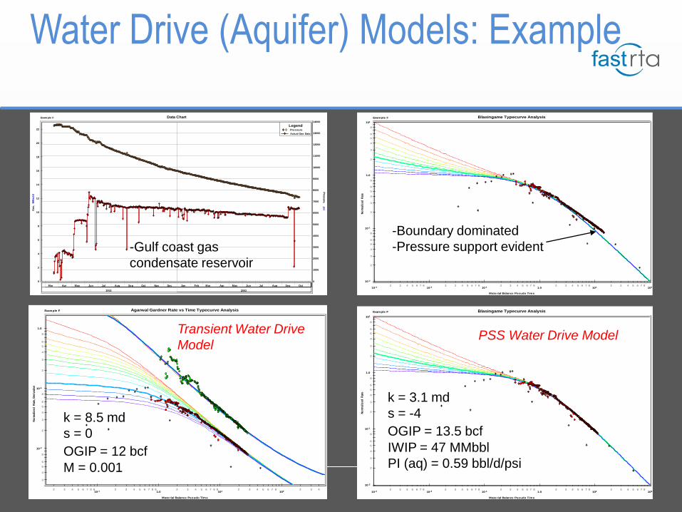
Water Drive (Aquifer) Models: Example
10-3 10-2 10-1 1.0 101 1022 3 4 5 6 7 8 2 3 4 5 6 7 8 2 3 4 5 6 7 8 2 3 4 5 6 7 8 2 3 4 5 6 7 8
Material Balance Pseudo Time
10-2
10-1
1.0
101
2
3
4
5
6
8
2
3
4
5
6
8
2
3
4
5
6
8
No
rmal
ized
Rat
e
Blasingame Typecurve AnalysisExample F
-Boundary dominated
-Pressure support evident
Mar Apr May Jun Jul Aug Sep Oct Nov Dec Jan Feb Mar Apr May Jun Jul Aug Sep Oct
2002 2003
0
2
4
6
8
10
12
14
16
18
20
22
Gas,
MM
scfd
0
1000
2000
3000
4000
5000
6000
7000
8000
9000
10000
11000
12000
13000
14000
Pre
ssu
re,
psi
Data ChartExample F
LegendPressure
Actual Gas Data
-Gulf coast gas
condensate reservoir
10-1 1.0 101 1022 3 4 5 6 7 8 9 2 3 4 5 6 7 8 9 2 3 4 5 6 7 8 9 2 3 4 5 6 7 8 2 3 4
Material Balance Pseudo Time
10-2
10-1
1.0
3
4
5
6
8
2
3
4
5
6
8
2
3
4
5
6
8
No
rmalized
R
ate
, D
eri
vati
ve
Agarwal Gardner Rate vs Time Typecurve AnalysisExample F
k = 8.5 md
s = 0
OGIP = 12 bcf
M = 0.001
Transient Water Drive
Model
10-3 10-2 10-1 1.0 101 1022 3 4 5 6 7 8 2 3 4 5 6 7 8 2 3 4 5 6 7 8 2 3 4 5 6 7 8 2 3 4 5 6 7 8
Material Balance Pseudo Time
10-2
10-1
1.0
101
2
3
4
5
6
8
2
3
4
5
6
8
2
3
4
5
6
8
No
rmalized
R
ate
Blasingame Typecurve AnalysisExample F
k = 3.1 md
s = -4
OGIP = 13.5 bcf
IWIP = 47 MMbbl
PI (aq) = 0.59 bbl/d/psi
PSS Water Drive Model

Multiple Well Analysis

1. Empirical- Group production decline plots
2. Material Balance Analysis- Shut-in data only
3. Reservoir Simulation
4. Semi-analytic production data analysis methods
- Blasingame approach
Multi-well / Reservoir-based Analysis-
Available Methods

Multi-Well Analysis- When is it
required?
1. Situations where high efficiency is required
- Scoping studies / A & D
- Reserves auditing
2. Single well methods sometimes don’t apply
- Interference effects evident in production / pressure
data- Wells producing and shutting in at different times
- Predictive tool for entire reservoir is required
- Complex reservoir behavior in the presence of
multiple wells (multi-phase flow, reservoir
heterogeneities)

Multi-Well Analysis- When is it not
required?
The vast majority of production data can be analyzed
effectively without using multi-well methods
1. Single well reservoirs
2. Low permeability reservoirs
- Pressure transients from different wells in reservoir
do not interfere over the production life of the well
3. Cases where “outer boundary conditions” do not change
too much over the production life of the well
- Wide range of reservoir types

Identifying Interference
Well A Well B
Rate is adjusted at Well A
q
Q Q
Response at Well B

Correcting Interference Using
Blasingame et al Method
A
BAtotce
qqt
Q
Define a “total material balance time” function
tce is used in place of tc to plot the data in the typecurve match
(for analyzing Well A)

Multi-Well Analysis as a
Typecurve Plot
log(q/Dp)
tce= (QB +QA)/qA
log(tc) tcA tce
MBT is corrected for
interference caused
by production from
Well B
Analysis of Well A:
Also applies to Agarwal-Gardner, NPI and FMB

Multi-Well Analysis- Example
1991 1992 1993 1994 1995 1996 1997 1998 1999 2000 2001 2002
0.00
0.50
1.00
1.50
2.00
2.50
3.00
3.50
4.00
4.50
5.00
5.50
6.00
Oil / W
ate
r R
ate
s,
bb
l/d
0.00
0.20
0.40
0.60
0.80
1.00
1.20
1.40
1.60
1.80
2.00
2.20
2.40
2.60
2.80
Gas,
MM
scfd
0
2000
4000
6000
8000
10000
12000
14000
16000
18000
20000
22000
24000
26000
28000
30000
32000
34000
36000
Pre
ssu
re,
psi
Data ChartWell 1
LegendPressure
Actual Gas Data
Pool Production
Water Production
-Three well system
-“Staggered” on-stream dates
-High permeability reservoir
Aggregate production of well group
Production history of well to be analyzed
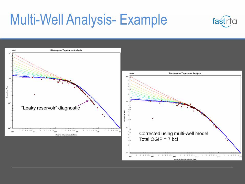
Multi-Well Analysis- Example
10-3 10-2 10-1 1.0 101 1022 3 4 5 6 7 8 2 3 4 5 6 7 8 2 3 4 5 6 7 8 2 3 4 5 6 7 8 2 3 4 5 6 7 8
Material Balance Pseudo Time
10-2
10-1
1.0
101
2
3
4
5
7
2
3
4
5
7
2
3
4
5
7
No
rmalized
R
ate
Blasingame Typecurve AnalysisWell 1
“Leaky reservoir” diagnostic
10-3 10-2 10-1 1.0 101 1022 3 4 5 6 7 8 2 3 4 5 6 7 8 2 3 4 5 6 7 8 2 3 4 5 6 7 8 2 3 4 5 6 7 8
Material Balance Pseudo Time
10-2
10-1
1.0
101
2
3
4
5
7
2
3
4
5
7
2
3
4
5
7
No
rmalized
R
ate
Blasingame Typecurve AnalysisWell 1
Corrected using multi-well model
Total OGIP = 7 bcf

Multi-Well Analysis- Example
0.00 0.40 0.80 1.20 1.60 2.00 2.40 2.80 3.20 3.60 4.00 4.40 4.80 5.20 5.60 6.00 6.40 6.80 7.20 7.60
Cumulative Production, Bscf
0
100
200
300
400
500
600
700
800
900
1000
1100
1200
1300
1400
1500
1600
1700
1800
1900
P/Z
*, psi
Flowing Material BalanceWell 1
Original Gas In Place
LegendP/Z Line
Flowing P/Z*
OGIP for subject well = 3.5 bcf
0.00 0.40 0.80 1.20 1.60 2.00 2.40 2.80 3.20 3.60 4.00 4.40 4.80 5.20 5.60 6.00 6.40 6.80 7.20 7.60 8.00
Cumulative Production, Bscf
0
200
400
600
800
1000
1200
1400
1600
1800
2000
P/Z
*, psi
Flowing Material BalanceWell 1
Original Gas In Place
LegendP/Z Line
Flowing P/Z*
Total OGIP = 7.0 bcf

Overpressured Reservoirs

1. Analysis methods are the same as normally pressured case
2. Additional parameters to be aware of
• Formation compressibility
• In-situ water compressibility
• Compaction effects (pressure dependent permeability)
3. Two models available, depending on required complexity
• p/z* model (accounts for constant cf, cw and co in
material balance equation
• Full geomechanical model (accounts for cf(p) and k(p))
Overpressured Reservoirs

Compresibilities of Gas and Rock
Compressibility vs. Pressure (Typical Gas Reservoir)
0.00E+00
5.00E-05
1.00E-04
1.50E-04
2.00E-04
2.50E-04
3.00E-04
0 2000 4000 6000 8000 10000 12000
Reservoir Pressure (psi)
Co
mp
ressib
ilit
y (
1/p
si)
gas
formation
Formation energy is critical in this regionFormation
energy may
be influencial
in this region
Formation
energy is
negligible in
this region

p/z* Model – Corrects Material
Balance
ca
0
( )
1 ( )
tt i
t f i
c q tt dt
q c c p p
*
11
1 ( )
1
i
i
p
f i
p
p p G
zz c p p OGIP
p p G
zz OGIP
Flowing MB
Typecurves

Geomechanical Model – Corrects
Well Productivity
D
4
3ln
*6417.1
)(
2 **
wa
e
i
a
iit
ip
r
r
hk
Tqet
GZc
qpp
Dpi
pwfi
p
z
pdppk
kp
)(2*
t
ti
ita
c
dtk
k
ct
0
* )(
where
In the standard pressure transient equations, permeability is usually considered to be
constant. There are several situations where this may not be a valid assumption:
1. Compaction in overpressured reservoirs
2. Very low permeability reservoirs in general
3. Unconsolidated and/or fractured formations
One way to account for a variable permeability over time is to modify the definition of
pseudo-pressure and pseudo-time.
Pressure dependent
permeability included in
pseudo-pressure and pseudo-
time

Overpressured Reservoirs -
Example
10-3 10-2 10-1 1.0 101 1022 3 4 5 6 7 8 2 3 4 5 6 7 8 2 3 4 5 6 7 8 2 3 4 5 6 7 8 2 3 4 5 6 7 8
Material Balance Pseudo Time
10-2
10-1
1.0
101
2
3
4
5
6
8
2
3
4
5
6
8
2
3
4
5
6
8
No
rmalized
R
ate
Blasingame Typecurve Analysis
Gulf Coast, deep gas condensate reservoir
Boundary dominated flow
OGIP = 17 bcf

Overpressured Reservoirs -
Example
June July August September October
2003
0
10
20
30
40
50
60
70
80
Rat
e,
MM
scfd
2000
4000
6000
8000
10000
12000
14000
16000
18000
Pressu
re, p
si
History Match
Radial Model218 Prod and Pressure Data
Good flowing pressure match,
Poor shut-in pressure match
OGIP = 17 bcf

Overpressured Reservoirs -
Example
June July August September October
2003
0
10
20
30
40
50
60
70
80
Rat
e,
MM
scfd
2000
4000
6000
8000
10000
12000
14000
16000
18000
Pressu
re, p
si
History Match
Radial Model218 Prod and Pressure Data
Good flowing pressure match,
Good shut-in pressure match
OGIP = 29 bcf
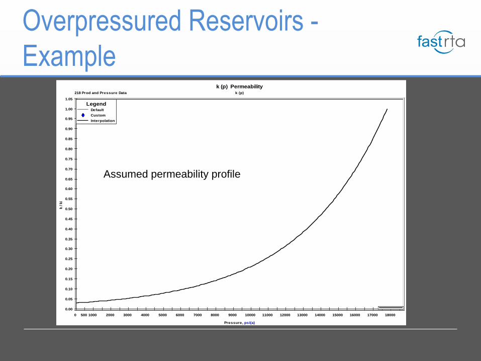
Overpressured Reservoirs -
Example
0 500 1000 2000 3000 4000 5000 6000 7000 8000 9000 10000 11000 12000 13000 14000 15000 16000 17000 18000
Pressure, psi(a)
0.00
0.05
0.10
0.15
0.20
0.25
0.30
0.35
0.40
0.45
0.50
0.55
0.60
0.65
0.70
0.75
0.80
0.85
0.90
0.95
1.00
1.05
k / k
i
k (p)
k (p) Permeability218 Prod and Pressure Data
LegendDefault
Custom
Interpolation
Assumed permeability profile

Horizontal Wells

Horizontal Wells
Horizontal wells may be analyzed in any of three different ways, depending on completion and petrophysical details:
1. As a vertical well,• if lateral length is small compared to drainage area
2. As a fractured well,• if the formation is very thin• if the vertical permeability is high• if the lateral is cased hole with single or multiple stage
fractures• to get an idea about the contributing lateral length
3. As a horizontal well (Blasingame model)• all others

Where is the square root of the anisotropic ratio:
Horizontal Wells – Blasingame
TypecurvesThe horizontal well typecurve matching procedure is based on a square shaped reservoir with uniform thickness (h).
The well is assumed to penetrate the center of the pay zone.
The procedure for matching horizontal wells is similar to that of vertical wells. However, for horizontal wells, there is
more than one choice of model. Each model presents a suite of typecurves representing a different penetration ratio
(L/2xe) and dimensionless wellbore radius (rwD). The definition of the penetration ratio is illustrated in the following
diagram:
L
rr
wawD
2
h
LLD
2
v
h
k
k
The characteristic dimensionless parameter for each suite of horizontal typecurves is defined as follows:
For an input value of “L”,
L
2xe
rwa h
Plan
Cross Section
L
2xe

Horizontal Wells – Example
10-3 10-2 10-1 1.0 101 1022 3 4 5 6 7 8 2 3 4 5 6 7 8 2 3 4 5 6 7 8 2 3 4 5 6 7 8 2 3 4 5 6 7 8
Material Balance Pseudo Time
10-2
10-1
1.0
101
102
2
3
4
6
8
2
3
4
6
8
2
3
4
6
8
2
3
4
6
8
No
rmalized
R
ate
Blasingame Typecurve AnalysisUnnamed Well
L/2xe = 1
rwD = 2e-3
Ld = 5
Le = 1,968 ft
k (hz) = 0.18 md
k (v) = 0.011 md
OGIP = 1.1 bcf

Oil Wells

Oil Wells
Analysis methods are no different from that
of gas reservoirs (in fact they are simpler)
provided that the reservoir is above the
bubble point
If below bubble point, a multi-phase
capable model (Numerical) must be used
Include relative permeability effects
Include variable oil and gas properties

Oil Wells – Example
Apr May Jun Jul Aug Sep Oct Nov Dec Jan Feb Mar Apr May Jun Jul Aug Sep Oct
2001 2002
0
10
20
30
40
50
60
70
80
90
100
110
120
130
140
150
160
170
180
190
Liq
uid
Rate
s,
bb
l/d
0.00
0.01
0.02
0.03
0.04
0.05
0.06
0.07
0.08
0.09
0.10
0.11
Gas,
MM
scfd
0
200
400
600
800
1000
1200
1400
1600
1800
2000
2200
2400
2600
2800
3000
3200
3400
3600
3800
4000
Pre
ssu
re,
psi
Data Chartexample7
LegendPressure
Actual Gas Data
Oil Production
Water Production- Pumping oil well
- Assumed to be pumped offProducing GOR ~ constant
(indicates reservoir pressure is above
bubble point

Oil Wells – Example
Rs input from production data,
Pbp and co calculated using
Vasquez and Beggs
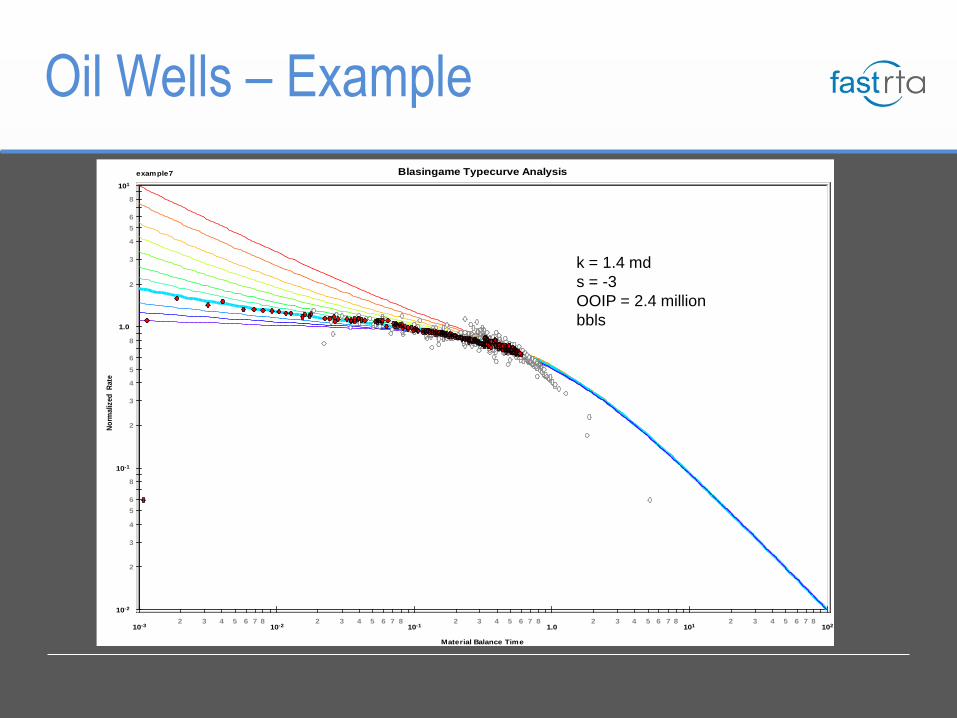
Oil Wells – Example
10-3 10-2 10-1 1.0 101 1022 3 4 5 6 7 8 2 3 4 5 6 7 8 2 3 4 5 6 7 8 2 3 4 5 6 7 8 2 3 4 5 6 7 8
Material Balance Time
10-2
10-1
1.0
101
2
3
4
5
6
8
2
3
4
5
6
8
2
3
4
5
6
8
No
rmalized
R
ate
Blasingame Typecurve Analysisexample7
k = 1.4 md
s = -3
OOIP = 2.4 million
bbls

Oil Wells – Example
2001 2002 2003 2004 2005 2006 2007 2008 2009 2010 2011 2012 2013 2014 2015 2016 2017 2018 2019 2020 2021 2022
0
20
40
60
80
100
120
140
160
180
200
220
240
260
280
300
Oil R
ate
, b
bl/d
0
200
400
600
800
1000
1200
1400
1600
1800
2000
2200
2400
2600
2800
3000
3200
3400
3600
3800
4000
Pre
ssu
re,
psi
Numerical Radial Model - Production Forecastexample7
LegendHistory Oil Rate
Flow Press
Syn Rate
History Reservoir Press
Forecasted Press
Forecasted Reservoir Press
Forecasted Rate
240 month forecast
EUR = 265 Mbbls