
Tolerance synthesis scheme - GPO Cylindrical Feature - Modified to MMC.....17 3.3.4 Cylindrical...
62
NISTIR 6836 Tolerance Synthesis Scheme U. Roy N. Pramanik H. Wang R. Sudarsan R. D. Sriram K. W. Lyons
Transcript of Tolerance synthesis scheme - GPO Cylindrical Feature - Modified to MMC.....17 3.3.4 Cylindrical...

Tolerance Synthesi
NISTIR 6836
s Scheme
U. RoyN. Pramanik
H. WangR. Sudarsan
R. D. SriramK. W. Lyons
NISTIR 6836
Tolerance Synthesis Scheme
U. RoyN. Pramanik
H. WangR. Sudarsan
R. D. SriramK. W. Lyons
June 03
U.S. DEPARTMENT OF COMMERCEDonald L. Evans, Secretary
TECHNOLOGY ADMINISTRATIONPhillip J. Bond, Under Secretary of Commerce for Technology
NATIONAL INSTITUTE OF STANDARDS AND TECHNOLOGYArden L. Bement, Jr., Director

Tolerance Synthesis Scheme
U. Roy, N. Pramanik and H. Wang Knowledge Based Engineering Laboratory Dept. of Mechanical , Aerospace, Manufacturing Engineering, Syracuse University Syracuse, NY 13244-1240 Email: {uroy, pramanik, hawang}@ecs.syr.edu
R. Sudarsan1, R. D. Sriram and K. W. Lyons Design and Process Group Manufacturing Systems Integration Division National Institute of Standards and Technology Gaithersburg, MD 20899 1 George Washington University Email: {sudarsan, sriram, klyons}@cme.nist.gov
Abstract The objective of this report is to identify representations and issues for the generic assembly information model and its use in a proactive tolerance synthesis scheme. It is proposed to use the small displacement torsors (the screw parameters) as a mathematical tool for analyzing the causal relationship between variations in parts’ shapes and sizes (due to the small allowances permitted by tolerance specifications), and their effects on relative positioning on adjacent parts. For a given assembly, the allowable geometric variations of assembled parts, the assembly specification and the desired functional requirements have been characterized by finite sets of equality and inequality constraints. An optimization process is then formulated to study the tolerance synthesis and analysis problems in the assembly.

Tolerance Synthesis Scheme Page 1 of 62
TABLE OF CONTENTS
Abstract .....................................................................................................................................................0 1. Introduction .......................................................................................................................................3 2. Tolerance Synthesis Scheme.............................................................................................................3 3. Generation of Constraints..................................................................................................................7
3.1 Constraints Related to Performance/ Functional Requirements................................................7
3.2 Constraints related to Assembleability / Kinematic Mating .....................................................8
3.2.1 Derivation of the A matrix ......................................................................................................8 3.3 Constraints related to mapping of tolerance to deviation parameters .....................................11
3.3.1 Representation of Geometric Deviations of Features of a Part .......................................12 3.3.2 Planar Features ................................................................................................................15 3.3.3 Cylindrical Feature - Modified to MMC.........................................................................17 3.3.4 Cylindrical Feature Modified to RFS..............................................................................20 3.3.5 Spherical Surface.............................................................................................................23 3.3.6 Conical Feature ...............................................................................................................25 3.3.7 Special cases....................................................................................................................28 Example of Some Mappings ...........................................................................................................32 Case 1: Planar Feature.....................................................................................................................32 Case 2: Cylindrical mating..............................................................................................................34
4. Optimization Process.......................................................................................................................35 4.1 Cost of Manufacturing ............................................................................................................35
4.2 Deviation-based Cost Model of Manufacturing......................................................................36
4.3 Optimization Process...............................................................................................................39
Acknowledgement...................................................................................................................................40 Disclaimer ...............................................................................................................................................41 References ...............................................................................................................................................41 Appendix – A: An Example of Deriving Assembliability Constraints ...................................................43 Appendix – B: Class diagrams of the basic entities in the synthesis scheme .........................................50 Appendix - C: Artifact Database Tables and Relations ........................................................................51
Page 1

Tolerance Synthesis Scheme Page 2 of 62
LIST OF FIGURES Figure 1: A spur gear sub-assembly ........................................................................................................4 Figure 2: Mating surfaces of the gear sub-assembly ...............................................................................5 Figure 3: Assembly Graph of the gear sub-assembly ............................................................................5 Figure 4: Points of interest on features. ...................................................................................................6 Figure 5: Transformation of Torsors – Local to Global...........................................................................8 Figure 6: Loops/Paths in an assembly ....................................................................................................10 Figure 7: Planar feature (rectangular) with size tolerance....................................................................15 Figure 8: Planar feature (circle) with size tolerance .............................................................................16 Figure 9: Cylindrical Feature with LCS .................................................................................................17 Figure 10: Cylindrical Feature with Tolerance Modified to MMC........................................................19 Figure 11: Cylindrical Feature with Tolerance Modified to RFS ..........................................................20 Figure 12: Cylindrical tolerance zone.......................................................................................................21 Figure 13: Derivation of constraint on Dqx ...........................................................................................22 Figure 14: Derivation of constraint on Dqy ...........................................................................................22 Figure 15: Spherical feature with LCS ..................................................................................................23 Figure 16: Spherical feature with tolerance specification......................................................................23 Figure 17: Conical feature with LCS......................................................................................................26 Figure 18: Conical feature with tolerance specification .......................................................................28 Figure 19: Composite tolerance specification .......................................................................................29 Figure 20: MMC Specified to datum......................................................................................................31 Figure 21: Planar feature (rectangular) with size tolerance.................................................................32 Figure 22: Deviation space for size tolerance on planar surface..........................................................33 Figure 24: Cost as function of deviation parameters .............................................................................38 Figure 25: Cost contour lines and the bounds........................................................................................38 Figure 26: Interacting torsors at mating surfaces ................................................................................44 Figure 27: Example problem with three blocks .................................................................................................46 Figure 28: Example problem with feature numbers and LCS ................................................................46 Figure 29: Block Artifact ........................................................................................................................56 Figure 30: Nominal shape with local coordinate systems (LCS)............................................................57 Figure 31: Feature to feature connectivity diagram...............................................................................57 Figure 32: Artifact Control main Screen ................................................................................................58 Figure 33: Sample cost of Manufacturing Function.......................................................................................58 Figure 34: Optimized configuration................................................................................................................59
Page 2

Tolerance Synthesis Scheme Page 3 of 62
1. Introduction
This report gives details of work on tolerance synthesis subsequent to our earlier work [ROY01]. For tolerance synthesis and analysis, we principally need a detailed description of the “kinematic functions” of the assembly, by which we mean those functions defined essentially by the location, size and shape (form) of associated mating features. These kinematic functional specifications are not directly provided by the customer or by early specifications of the desired product / assembly function. They are slowly evolved with the assembly as the design takes concrete shape and size in the later phases of the conceptual design. Tolerance synthesis and analysis needs an exhaustive functional analysis mechanism to make sure that the identified functional requirements between the mating components of the assembly are met and are suitably described in the form of critical toleranced dimensions / size / sizes / forms or in the form of toleranced gaps. The tolerance representation procedure uses the small deviation torsor scheme [BAL00] to represent the variations associated with each feature of a part in the assembly. The tolerance representation and synthesis scheme has been elaborated in the following Section 2. Section 3 discusses the formulation of cost functions while Section 4 presents a detailed discussion on the several constraint generation procedures for establishing the optimization process as described in section 5. Section 6 briefly describes the implementation issues with an example.
2. Tolerance Synthesis Scheme
Based on the considerations discussed in earlier works, we propose the following steps for the tolerance synthesis scheme: 1. For each component of the artifact, develop the kinematic Degrees Of Freedom (DOF)
requirement between the mating features and decide the intrinsic displacement and deviation of the surface from the nominal surface as torsor components.
2. For each pair of connected features, establish the gap between the features as a gap torsor
taking into account the indeterminate and/or blocked degrees of freedoms. 3. Generate assembleability constraints by considering all chains of connected components as a
kinematic link (either closed loop or path between two datum features) and aggregate the torsors along the path with reference to a global frame of reference. Each loop would generate a maximum possible of six equations binding the deviation parameters associated with all the related surfaces. These sets of constraints would form a deviation for the possible geometric variations of the connected components.
4. Generate functional requirement constraints based on the specified functions/objectives to be
fulfilled by the artifact. This will restrict the range of values of the deviations within which a component must remain to fulfill specific functional requirements.
5. Generate manufacturing / production cost models for each component (based on a suitable
knowledgebase for manufacturing/ production costs) for different machining operations, and
Page 3

Tolerance Synthesis Scheme Page 4 of 62
formulate a minimization scheme by considering the sum of costs for machining all the parts as the cost function subject to the constraints defined in steps 3 and 4.
6. Use standard mathematical tools to solve the above optimization scheme to find the deviation
parameters for each component. Convert the deviation parameters associated with each surface into appropriate tolerance zones through a tolerance mapping scheme.
Let us take an example to elaborate the steps described above for the tolerance synthesis process. The example has been taken from the design evolution solution in our earlier work [ROY01] where we illustrated the design evolution process by taking an example of designing a device for transmitting torque with changing rotational speed. We used a sample artifact library and arrived at a few tentative design solutions that matched the functional requirements. We take one of the solutions from the above design example and assume the tentative sizing of the components. The gear-subassembly consists of three parts: a spur gear, a shaft with a keyhole and a key. The geometric models of these three parts, including their face-level mating relationships and behavioral models have been shown in Figure 1, Figure 2.
Key
Gear
Shaft
Figure 1: A spur gear sub-assembly
Page 4

Tolerance Synthesis Scheme Page 5 of 62
Part 2: Gear Hub P2F3 P3F2 P2F2 P2F4 P2F1 Part 3: Key P3F1 P3F3 P1F1 P1F2 P3F4 P1F4 P1F3 Part 1: Shaft
Figure 2: Mating surfaces of the gear sub-assembly
F1 F4 F1 F2 F2 Part 1 F4 F3 Part 2 F3
F1 F2 F4 Part 3 F3
Figure 3: Assembly Graph of the gear sub-assembly
After the torsors for each of the mating surfaces have been defined, we consider the assembly graph of the artifact (Figure 3) and enumerate closed loops of independent paths for forming equations that represent various possible geometric configuration hulls for the artifact. Thus, for example, a typical closed loop from the Figure 3 would be represented by: T[F1/P1] Gap[F1/P1,F1/P2] T[F1/P2,F4/P2] Gap[F4/P2,F3/P3] T[F3/P3] Gap[F3/P3,F4/P1] T[F4/P1] T[F1,P1]. (Please see appendix –A for details). The aggregation of these torsors (transforming into global reference frame, as needed) should then be equated to a null torsor. This will give six equations connecting the components of the torsors associated with the loop. The gap between the mating features will be used as constraints to satisfy specific design functional requirements as well as kinematic requirements.
Page 5

Tolerance Synthesis Scheme Page 6 of 62
For computations in each loop, the local variations are to be converted to a global coordinate system by transformation of the corresponding torsors in the local frame. Thus, in the case of this example, in, we can take the center of the inner shaft as the reference origin and express all the components in terms of vectors emanating from that point. While traversing these loops, the gap between the two mating features would play a vital role in deciding the type of interface between the two mating features. The gap torsor is required to model the kinematic/ functional specifications specific to the given mating conditions. However, we also need to assess the possibility of any interference between the mating features by applying the torsor on some specific points on the two mating features. This would require studying the torsor equations applied on those strategic points. These strategic points could be some inspection points to be used in future inspection of the features. We have kept points of kinematic interest in the artifact class definition so that we can create those points as required on specific surfaces/features. As an example, in case of a rectangular feature, we can select the four furthest points (corner points) as the desired points. For circular features, we can keep eight points uniformly placed on the circumference (Figure 4). It may be mentioned that additional points as desired may be introduced at any stage to improve accuracy; however, the number of equations and complexity of the problem would increase with each additional point.
Rectangular: 4 points (At the end of each diagonal) A Circular: 8 points @ equal intervals 0
Figure 4: Points of interest on features.
After all the loops have been considered and corresponding equations have been formed, we will get a system of equations that will define the possible geometric variations of the artifact configuration. Depending on the type of mating and functional requirements for each mating pairs of surfaces, these sets of equations may be under or over constrained. In other words, there may be too few equations connecting too many variables or vice-versa. These will constitute the constraints of the optimization process for tolerance synthesis.
The proposed optimization scheme could be now summarized as below: Minimize: Cost of manufacturing
Page 6
Tolerance Synthesis Scheme Page 7 of 62
Subject to: Constraints associated with the geometry of the product as imposed by the kinematic
requirements between mating features and the constraints associated with functional requirements.
In the following sections, we will detail:
i) Model for cost of manufacturing ii) Constraints related to Performance/Functional requirements iii) Constraints related to Assembleability/Kinematic Mating iv) Constraints related to mapping of tolerance to feature deviation parameters, and v) Optimization process, and other implementation issues
3. Generation of Constraints
We have considered two types of constraints associated with the tolerance synthesis process. Constraints arising to meet the functional requirements and constraints associated with the kinematic mating requirements / assembleability. Since both the constraints play a crucial role in the tolerance synthesis process, we have elaborated each process separately in the following sub-sections.
3.1 Constraints Related to Performance/ Functional Requirements Functional requirements are design requirements specified explicitly as well as implicitly by the user and designers to meet a certain desired performance from the artifact/assembly. In terms of low-level tolerance and deviation parameters the functional requirements would translate into constraint i.e. functions establishing some relationship between parameters. These relations could be of two types: equality and inequality. The functional requirements can be thought of in two different ways: as a goal satisfaction to minimize a penalty cost for deviating from the design specification or to convert the functional requirements as a set of constraints on the tolerance zone. Since the functional requirements are developed based on customer’s specification and designer’s technical requirements, it is desirable to satisfy the product specification / functional requirements as necessary constraints rather than a goal satisfaction process. Thus, we have decided to treat the functional requirements as constraints on the geometric variations of the mating features of the components and considered manufacturing cost as a minimization goal to arrive at an optimal tolerance design. We need to develop a generic process to transform the functional requirements associated with a design into corresponding set of constraints. The functional requirements mainly translate into algebraic inequalities representing constraints of the form:
G(x) ≤ 0, x ∈ Rn. (3.1-1)
Functional requirements specified between two mating features could be represented by using the gap torsor parameters associated with each mating. A Functional requirement can be thought of in two different ways: either as a goal satisfaction to minimize a penalty cost for deviating from the design specification or as a set of constraints on the tolerance zone.
Page 7

Tolerance Synthesis Scheme Page 8 of 62
We are working to evolve a generic approach to transform the functional requirements associated with a design into a corresponding set of constraints. We have already introduced some treatment of functional requirements and constraints in our earlier work [ROY01] and we need to extend further the work done to transform the constraint equations as functions of the deviation parameters.
3.2 Constraints related to Assembleability / Kinematic Mating The constraints arising from the kinematic requirements between the mating surfaces to meet the requirement of transmission and/or blocking the desired flow of energy / force / fluent / information through the mating area could be treated as kinematic constraints. The torsor scheme for the modeling of the small geometric variations of connecting features / faces of an artifact has been adopted for the present study and the scheme has been elaborated in our earlier report [ROY00b]. These kinematic assembleability constraints are established by considering the sum of the torsor components along each independent paths/loops that exist between datum surfaces. The torsor summation is carried out using the torsor transformation rules by transferring the effect to a global point on the datum surface. In our assumed model with small displacements / deviations, the assembleability constraints become linear and can be put into the compact form: Ax = b, where A = [aij] an m x n matrix, aij ∈ R, x ∈ Rn
, b ∈ Rm , m is the number of constraints and in general m is less than number of deviation parameters n. We would need to work further to establish an automated process to generates the A matrix from the specified assembly configuration.
3.2.1 Derivation of the A matrix Since we will the need torsor transformations in the derivation of the A matrix, the torsor transformations are presented below (Figure 5). Transformation of Torsors
Figure 5: Transformation of Torsors – Local to Global
z
N
y
x
Z M
z y
x
Y
X
Page 8

Tolerance Synthesis Scheme Page 9 of 62
A small deviation torsor (SDT) TN defined at a point N in the local coordinate system (x, y, z) with six components (θx, θy, θz, δx, δy , δz) (where θ denotes rotational and δ denotes linear components of movements) transforms to (TN)ML (where L denotes local coordinate system) in the same local coordinate system shifted to a new point M is be given by: (TN)ML = (θx, θy, θz, δx + (θy*∆z - θz *∆z), δy + (θz *∆x – θx *∆z), δz + (θx *∆y – θy *∆x)) . This could be written in compact notation as: (TN)ML = DTN where D is the 6x6 transformation matrix given by
,
100001000010000100000010000001
∆∆−∆−∆∆∆−
=
xyxz
yzD
(3.2.1-1)
where ∆ =(∆x, ∆y, ∆z)T = (XN-XM, YN -YM, ZN-ZM)T is the vector from point M to N in global coordinate system (X, Y, Z). After the above transformation, the components of torsor (TN)ML are still in the local coordinate system (x,y,z). Let the local coordinate system (x,y,z) be defined by the three unit vectors x = (kxX, kxY, kxZ), y = (kyX, kyY,kyZ) and z = (kzX, kzY, kzZ) in the global coordinate system, in other words, the local coordinate system could be represented by the [K] matrix given by:
. (3.2.1-2) [ ]
=
zZyZxZ
zYyYxY
zXyXxX
kkkkkkkkk
K
The components of (TN)ML could then be converted to the global system by the following transformation (applicable for both the linear movement and the small rotations in the sense of SDT) :
θ X = θx * kxX + θy * kyX + θz * kzX,, (3.2.1-3) θY = θx * kxY + θy * kyY + θ z* kzY , (3.2.1-4) θZ = θx * kxZ + θy * kyZ + θz* kzZ , (3.2.1-5) θG = [θ X θ Y θ Z]T = [K][ θx θy θz]T, θG = [K] θL. (3.2.1-6)
where the subscripts G and L refer to global and local coordinate systems respectively.
δX = [δx + (θy *∆z - θz*∆y)]* kxX + [δy+ (θz*∆x – θx*∆z)]* kyX + [δz+ (θx*∆y – θy *∆x)]* kzX , (3.2.1-7) δY = [δx + (θy *∆z - θz*∆y)]* kxY + [δy+ (θz*∆x – θx*∆z)]* kyY + [δz + (θx*∆y – θy*∆x)]* kzY, (3.2.1-8) δZ = [δx + (θy *∆z - θz*∆y)]* kxZ + [δy+ (θz*∆x – θx*∆z)]* kyZ + [δz + (θx*∆y – θy*∆x)]* kzZ, (3.2.1-9)
δG = [δX δY δZ]T = [K] ( [δx δy δz]T + [∆x ∆y ∆z]T × [θ z θ y θ z]T). (3.2.1-10) where × is the vector cross product.
Page 9

Tolerance Synthesis Scheme Page 10 of 62
δG = [K] ( δL + ∆ × θ L ) where ( δL = [δx δy δz]T , ∆ =(∆x, ∆y, ∆z)T, θ L = [ θx θy θz]T ). Combining the two transformations, we can write the result as: (where subscript G refers to global) (TN)MG = (θG, δG )
(TN)MG = ([K][ θx θy θz]T , [K] ( [δx δy δz]T + [∆x ∆y ∆z]T × [θ x θ y θ z]T ). (3.2.1-11)
The above relation could be written as (TN)MG = K2 (TN)ML , (3.2.1-12) where K2 is the 6 x 6 transformation matrix generated from (3.2.1-10). We will have to use above results for transforming each torsor (defined in the local coordinate system) in a loop to the global reference point before they can be combined. For each loop/cycle in the assembly graph (parts connected through mating of features), we would have (at most) six equations by summing all the deviations along a cycle/loop to zero (or a pre-assigned quantity). In this derivation, we will use following notation. Without any loss of generality and without any ambiguity we will assume that each loop/path could be enumerated as a linked list L defined by:
L = { (p, f), g, [(f, p, f), g]…, (f, p)}, (3.2.1-13) where p = part, f = feature, g = gap between mating features. Symbolically this can be represented as shown in Figure 6. Items within [ ]… could be repeated zero or more times as required to traverse a loop/path, (p, f) is the starting point (from_part, from_feature), (f, p) the end point (to_feature, to_part), [(f, p, f), g] are intermediate connections (to_feature, part, from_feature), gap along the path to the next part. Part Feature Gap Feature Part Feature Gap Feature Part
Figure 6: Loops/Paths in an assembly
Zero or more repetitions
In case of a closed loop, the last part would be the same as the first part. Both the starting and the final parts for open loops should be terminals (datums). In the case of closed loops, the summation of the torsors would be null (0), whereas for an open path, the summation would be equal to a torsor (possibly non-null) that has to be established from known functional specifications between the two terminal parts. We will designate this quantity as b. We will use T to indicate torsor with index p, f, g for parts, features and gaps respectively.
Page 10

Tolerance Synthesis Scheme Page 11 of 62
Pj = Part number j, j =1 to n, n = number of parts in the loop,
Fk = Feature k of part Pj , k = 1 to m, m = number of features of part Pj,
Tp = 6-component displacement torsor of the part P, defined at a suitable point O inside the part in a
local coordinate system, Tf = 6-component deviation torsor of the feature k (of some part Pj) , defined at a suitable point N on
the feature in a local coordinate system with x-axis along the outward (away from the material) normal and y and z are the other two axes mutually perpendicular to the x-axis,
Tg = 6-component gap torsor defined at a mating between two features of two parts.
With the above notation, we can write the desired equations for each loop, with implied local to global transformations applied to each torsor as viewed from any convenient point (typically, at the center of the first part where the loop begins), as:
(Tp + Tf ) + Tg [+ (Tf + Tp + Tf + Tg )]… + (Tf + Tp ) = b. (3.2.1-14)
Summing over the entire loop, we can write,
,)(* ∑
∈
=×∆+EntireLoopj
jjjj bxK δθδ (3.2.1-15)
,*
θθ bKEntireLoopj
jj =∑∈
(3.2.1-16)
where,
Kj is the local to global transformation matrix (eqn. (3.2.1-2) ) for feature j, δj = [δx δy δz]T
j and θ j = [θ z θ y θ z]Tj are the two vectors formed from the linear and
rotational components respectively of the deviation torsor of the feature j. The scheme for the representations and transformations of the torsors have been elaborated in Appendix – A with an example of an artifact with three blocks. Since the proposed scheme uses six small displacement parameters to represent the possible geometric deviations from the design / nominal surface, we need a mechanism to express standard tolerances in terms of these torsor parameters. We consider some engineering features/surfaces and develop the tolerance to deviation mappings in the following section.
3.3 Constraints related to mapping of tolerance to deviation parameters
Page 11
Tolerance Synthesis Scheme Page 12 of 62
The category of relations arising from the mapping of the deviation parameters of the features to corresponding tolerance values is of the generic non-linear inequality (“less than or equal to” type) and takes the form: FDP
k (x) ≤ FTol
k (t), where FDP is some function of the deviation parameters x∈Rn, FTol
is some function of the tolerance parameters t, and k∈ N+ is an index. Exact forms of FDP
k(x) and FTol
k(t), depend on the nature of the feature/surface. For a planar surface, the above relationship becomes a set of linear constraints. The interesting feature in the above relationship is the separable nature of the equation in terms of the variables t and x. We would like to explore the possibility of taking advantage of the separable nature of the mapping to define the deviation hull in a semi-analytical way, if possible. The linear nature of the equations, however, does not exist when we consider other non-planar features. So far, we have been successful in establishing the required relationships for the features: rectangular planar, circular planar, cylindrical, and spherical. Following sections give the detailed results.
3.3.1 Representation of Geometric Deviations of Features of a Part The geometric variations of the features are defined in terms of deviations of their independent degrees of freedom. In this approach, at the most six independent parameters would be used to represent a six-component vector corresponding to the possible six degrees of freedom. In actual case, depending on the type of surface (planar, cylindrical, etc) some of the degrees of freedom are ‘free’ (variations along which keeps the surface invariant) and thus, in general, less than six deviation parameters are required. For example, for a planar surface, rotation along the outward normal to the surface and movements along the two axes on the surface keep the feature invariant and hence a planar surface requires three deviation parameters (axial movement, two rotations along the two transverse axes). In order to make the process of converting the functional requirements as well as kinematic requirements into a set of constraints in a generic manner, we need a procedure to represent the variations associated with each part in terms of a set of generic parameters of the mating features/surfaces. Assuming small displacements/deviations of these features due to manufacturing inaccuracies/other defects, the actual surface of a feature deviates from the theoretical (nominal) surface slightly. Such variations could be systematically treated by considering variations of six small parameters defined at a point on the surface. The six parameters are: three linear translations and three rotations along the three axes of the local orthogonal coordinate system corresponding to the six degrees of freedom. These six small displacement parameters have been called screw parameters or torsors. Since the proposed method uses six small displacement variation parameters to represent the possible geometric deviations from the design / nominal surface, we need a mechanism to express geometric variations in terms of these torsor parameters. It has been mentioned above that not all the six parameters for each surface may be uniquely defined and we may not need to know all the six parameters in specific cases. We plan to consider each type of engineering surfaces and formulate methods to represent the tolerance values as functions of the parameters. This task require a mapping of the deviation parameters to geometric tolerances. So far, we have completed mappings for Planar, Cylindrical, and Spherical features. Conical, Toroidal, and Helical cases will be taken as future work. In order to give a meaningful interpretation to the assemblability of an artifact in terms of tolerance specifications as per industry standard codes and practices like ASME Y14.5.1M-1994, ISO, we need
Page 12

Tolerance Synthesis Scheme Page 13 of 62
to consider relationship between the tolerance zones (or virtual condition boundaries) and the deviation parameters of a feature. By deviation parameters, we mean the representation of the possible deviation of a feature by using (at most) six independent parameters corresponding to the six degrees of freedom of a feature. In general, the deviation parameters to tolerance mappings are not one-to-one and can only be represented as inequalities involving functions of the tolerance parameters and the deviation parameters. Mappings developed from these are, in general, a set of non-linear inequalities. However, for some specific cases, like the planar surface, the inequalities are linear, and represent a diamond shaped zone by the intersection of inequalities, each of which are half-spaces in the D x T (D: Deviation, T: Tolerance) space [BAL98]. There are four types of tolerances used in the industry: size tolerance, form tolerance, orientation tolerance, and location/position tolerance. These tolerances are sometimes specified with material conditions as modifiers. There are three such material conditions: MMC (Maximum Material Condition), LMC (Least Material Condition) and RFS (Regardless of Feature’s Size). Since we assume that the shape of a toleranced feature remains similar to the nominal feature (for example, a plane remains a plane, a cylinder remains a cylinder, etc.), the variation of position and orientation due to form tolerance is very small [Gil91] and in this study, we consider only the size tolerance, orientation tolerance, and positional tolerance. A geometric tolerance applied to a feature of size and modified to MMC will establish a virtual condition boundary (VCB) 4 outside of the material space adjacent to the feature. The feature shall not cross this VCB. Likewise, a geometric tolerance applied to a feature of size and modified to LMC establishes a VCB inside the material and the feature shall not cross the VCB. This translates to the following relationships [DRA99]: Modified to MMC:
For an internal feature of size: MMC virtual condition = MMC size limit – geometric tolerance; (3.3.1-1)
For an external feature of size: MMC virtual condition = MMC size limit + geometric tolerance; (3.3.1-2)
Modified to LMC: For an internal feature of size:
LMC virtual condition = LMC size limit + geometric tolerance; (3.3.1-3) For an external feature of size:
LMC virtual condition = LMC size limit – geometric tolerance. (3.3.1-4) If a geometric tolerance applied to a feature of size is neither modified to MMC nor LMC, by definition of standards such as ASME Y14.5, it is modified to RFS. In this case, instead of VCB, the tolerance specification will generate a tolerance zone into which the derived element will not interfere. A VCB or tolerance zone represents the basic intention of the designer that each point on the toleranced feature/derived element should remain within (or outside) this boundary/zone. Hence, the VCB or tolerance zone would be ideally suitable for representing the relational limits on the deviation parameters associated with the deviation of the feature from its nominal position. Since the deviation parameters for a feature could be used to define the deviation of all points on a feature (by employing 4 Virtual condition boundary: A constant boundary generated by the collective effects of a size feature’s specified MMC or LMC material condition and the geometric tolerance for that material condition.
Page 13

Tolerance Synthesis Scheme Page 14 of 62
one or more independent parameters), the tolerance specifications could be thought of a set of limits for the deviation parameters and vice-versa. These relationships could be used for tolerance synthesis as well as for tolerance analysis including checking the assemblability in the worst-case scenario. In the following sections of this paper, we consider the mapping for size tolerance, positional tolerance, and orientation tolerance for four types of features: planar, cylindrical, spherical, and conical. For the planar case, there is no material condition as it is a non-size feature. For the cylindrical feature we have two cases: MMC and RFS and for the spherical feature we have MMC and for conical feature we have the size tolerance only. We use the following basic steps to convert a tolerance specification into a set of inequalities in the deviation parameters: a. Generate the intrinsic torsor and the deviation torsor for the feature by eliminating the deviation
parameters that are invariant for the feature to reduce the degrees of freedom. This reduces the number of deviation parameters needed to represent the variation of the feature. For example, for a cylindrical feature, axial movement and axial rotation are two invariants. Hence, we do not need these two parameters.
b. Generate a VCB (or a tolerance zone) based on the tolerance specification. In this step, we
compute the size of the VCB or the tolerance zone for restricting the variation of the feature or derived element respectively.
c. In case of VCB, take an arbitrary point on its nominal surface of the feature in a parametric
form and transform it to a new position by applying the effect of the deviation torsors. For example, for a cylindrical feature a point P on its nominal surface is represented by two parameters (θ, z); P = (rcosθ , rsinθ, z), where θ∈(0, 2π) and z ∈ (0, L), L=Length of the cylinder. In the case of tolerance zones, transform the derived element, such as center plane, center axis etc., to a new position by applying the effect of the deviation torsor.
d. Eliminate the free parameters, (such as the (θ, z) mentioned in step c above), by applying the
condition that the extreme points of the transformed position should remain within the VCB or that the derived element should remain within the tolerance zone. This step generates a set of inequalities connecting the deviation parameters with the tolerance specification.
The procedure for applying the above four steps will be clear in subsequent sections where we generate the mappings for the basic features under various material conditions The symbols used in the following sections, unless otherwise specified, are defined as below:
TU = Upper limit, size tolerance, TL = Lower limit, size tolerance, TP = Positional tolerance, TV = Perpendicularity tolerance, (∆θx, ∆θy, ∆θz, ∆x, ∆y, ∆z) = six components of the deviation torsor.
Page 14
Tolerance Synthesis Scheme Page 15 of 62
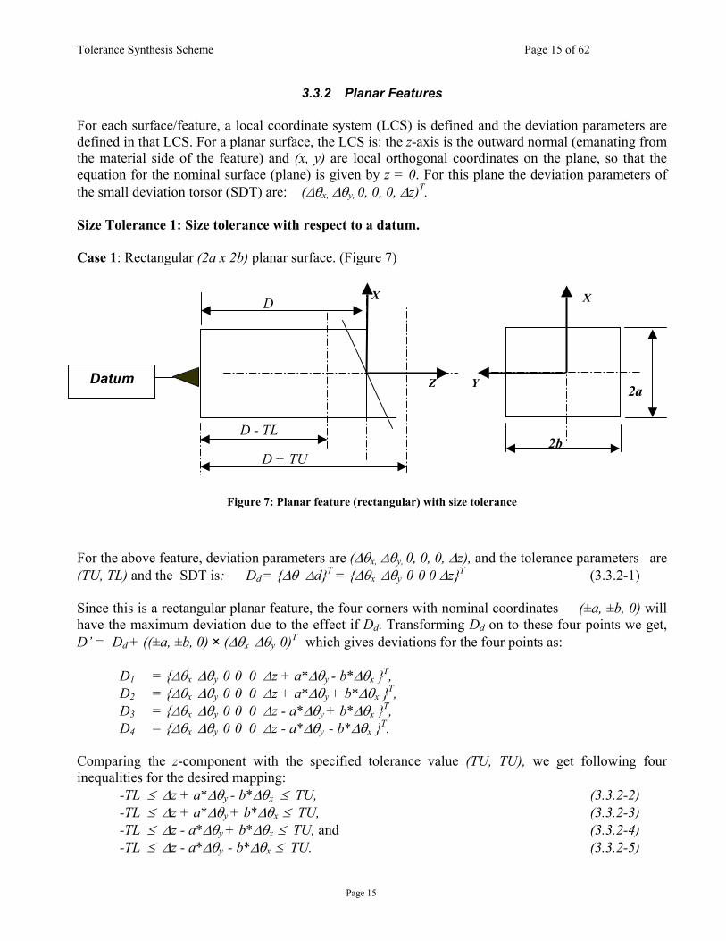
3.3.2 Planar Features For each surface/feature, a local coordinate system (LCS) is defined and the deviation parameters are defined in that LCS. For a planar surface, the LCS is: the z-axis is the outward normal (emanating from the material side of the feature) and (x, y) are local orthogonal coordinates on the plane, so that the equation for the nominal surface (plane) is given by z = 0. For this plane the deviation parameters of the small deviation torsor (SDT) are: (∆θx, ∆θy, 0, 0, 0, ∆z)T. Size Tolerance 1: Size tolerance with respect to a datum. Case 1: Rectangular (2a x 2b) planar surface. (Figure 7)
Figure 7: Planar feature (rectangular) with size tolerance
D + TU
D - TL
X
Z Y
2b
2a
X D
Datum
For the above feature, deviation parameters are (∆θx, ∆θy, 0, 0, 0, ∆z), and the tolerance parameters are (TU, TL) and the SDT is: Dd = {∆θ ∆d}T = {∆θx ∆θy 0 0 0 ∆z}T (3.3.2-1) Since this is a rectangular planar feature, the four corners with nominal coordinates (±a, ±b, 0) will have the maximum deviation due to the effect if Dd. Transforming Dd on to these four points we get, D’ = Dd + ((±a, ±b, 0) × (∆θx ∆θy 0)T which gives deviations for the four points as:
D1 = {∆θx ∆θy 0 0 0 ∆z + a*∆θy - b*∆θx }T, D2 = {∆θx ∆θy 0 0 0 ∆z + a*∆θy + b*∆θx }T,
D3 = {∆θx ∆θy 0 0 0 ∆z - a*∆θy + b*∆θx }T,
D4 = {∆θx ∆θy 0 0 0 ∆z - a*∆θy - b*∆θx }T. Comparing the z-component with the specified tolerance value (TU, TU), we get following four inequalities for the desired mapping:
-TL ≤ ∆z + a*∆θy - b*∆θx ≤ TU, (3.3.2-2) -TL ≤ ∆z + a*∆θy + b*∆θx ≤ TU, (3.3.2-3)
-TL ≤ ∆z - a*∆θy + b*∆θx ≤ TU, and (3.3.2-4)
-TL ≤ ∆z - a*∆θy - b*∆θx ≤ TU. (3.3.2-5)
Page 15

Tolerance Synthesis Scheme Page 16 of 62
Case 2: Circular (radius r) planar surface. (Figure 8)
Figure 8: Planar feature (circle) with size tolerance
β
D + TU
D - TL
X
Z
Y
X P
Datum
Deviation parameters = (0, 0, ∆z, ∆θx, ∆θy, 0), tolerance parameters = (TU, TL). For arbitrary point P on the circumference, at an angle β with the y-axis, we have, δz = ∆z -R∆θySin(β)+R∆θxCos(β), where δz is the pure position variation of a point in the Z direction, where there is a size tolerance control. The tolerance zone in this case is made up of two planes, z = +TU and z = -TL. We need to ensure that δz is within the above boundary ∀β ∈ (0, 2π) This can be done by treating the δz as a function of β and then finding the extreme points by putting ∂(δz )/ ∂β = 0. This gives,
δz max/min = ∆z ± R√( ∆θx2
+∆θy2).
This leads to the following mapping (constraints):
(∆θx
2 + ∆θy
2) ≤ (TU + TL)2/(4R2).
We can also write in the parametric form as
TL ≤ ∆z + R∆θxSin(β) + R∆θyCos(β) ≤ TU , ∀β ∈ (0, 2π). The last inequality, using the value of δz max/min could be written, independent of β, as:
Page 16

Tolerance Synthesis Scheme Page 17 of 62
TL ≤ (∆z - R√( ∆θx2
+∆θy2) ) and (∆z + R√( ∆θx
2 +∆θy
2) ) ≤ TU .
3.3.3 Cylindrical Feature - Modified to MMC Let us assume a cylindrical feature with a given tolerance specification as shown in Figure 9. A local coordinate system (LCS), as shown in Figure 10, is defined for cylindrical surface and the deviation parameters are defined in that LCS. For a cylindrical surface, the LCS is: z-axis along the axis of the cylinder and (x, y) are local orthogonal co-ordinates on the middle of the axis (Figure 9, Figure 10). For this surface, the deviation parameters of the SDT are: (∆x, ∆y, 0, ∆θx, ∆θy, 0) and dr. Based on this notation, constraints could be derived connecting these parameters with the specified tolerance values as detailed below. Deviation parameters = (∆x, ∆y, 0, ∆θx, ∆θy, 0), tolerance parameters = (TU, TL, TP ), SDT is:
Dd = {∆θ ∆d} = {∆θx ∆θy 0 ∆x ∆y 0}T, Di = {∆θ ∆d} = {0 0 0 dr*cosθ dr*sinθ 0}T , where Dd is displacement torsor5 and Di is intrinsic torsor6.
Let us assume that there is a point P ) ,sin ,cos( zrr θθ (Figure 9) on the nominal cylindrical surface. After applying the transformation due to the effect of the two small displacement torsors, the new position of transformed point P’ can be calculated as follows.
Figure 9: Cylindrical Feature with LCS
P’
Pz
yx
P
5 Displacement torsor: torsor for the deviation of the feature from the nominal position. 6 Intrinsic torsor: torsor to represent the intrinsic variation of size of the feature.
Page 17

Tolerance Synthesis Scheme Page 18 of 62
+∆++∆−∆+∆−+∆+∆++
=
++
∆∆−∆∆−∆∆
1sin)(cos)(
sin)(cos)(
1
sin)(cos)(
100001
1001
θθθθθθθθ
θθ
θθθθ
drrdrrzyzdrrxzdrr
zdrrdrr
yx
xy
x
y
xy
x
y
.
The 4 by 4 matrix on left hand side of the equation is the transformation matrix for point P following the assumed transformation sequence ∆x ∆y ∆θx ∆θy by displacement torsor. The 4 by 1 matrix (vector) on the left hand side of the equation represent the changed position of point P by intrinsic torsor. So, the new position P’ (Figure 9) is given by
).sin)(cos)( , sin)(, cos)(( θθθθθθθθ drrdrrzyzdrrxzdrr xyxy +∆++∆−∆+∆−+∆+∆++
The VCB of the cylindrical surface is constructed by using the rules (3.3.1-1, 3.3.1-2,3.3.1-3,3.3.1-4) and has the following properties:
o A perfect shape as that of the nominal cylindrical feature, o A size (diameter) of max size plus geometric tolerance, because its external feature and the
positional tolerance is modified to MMC, o A perfect orientation as that of the nominal cylindrical feature (vertical to C), o A perfect location as that of the nominal cylindrical feature.
Hence, the constraint equation will be:
4/Tp)TU2r()sin)(()cos)(( 222 ++≤∆+∆−++∆+∆++ yzdrrxzdrr xy θθθθ , (3.3.3-1) where θ ∈ (0, 2π). The left hand side is a function of two independent parameters θ and z ∈ (0, L). The inequality should be valid ∀θ ∈ (0, 2π) and ∀z ∈ (0, L). We thus need to eliminate θ and z from the LHS of (3.3.3-1) by finding the maximum of the above equation. LHS of equation (3.3.3-1) could be written as:
)33.3.3(
.0,)(1
min,0,)(1
max
get, ,0 ,0
zero, tof of sderivative partial theequatingBy
. , , , ,where)23.3.3( ,)sin()cos(),(
22
2
22
22
min22
2
22
22
max
22
−
+
+−+
+
±
=
+
+−+
+
±
=
=∂∂
=∂∂
∆=∆−=∆=∆=+=−+++++=
bd
cdbeabadbdf
bd
cdbeabadbdf
wezfandf
yedxcbdrraedzacbzazf
xy
θ
θθθθθ
Page 18

Tolerance Synthesis Scheme Page 19 of 62
Figure 10: Cylindrical Feature with Tolerance Modified to MMC
Virtual condition boundary
C
TUTLr ±2φ
B
A
The final set of constraints is:
.
,2
2 2
max
TUdrTL
TpTUrf
≤≤−
++
≤
When the toleranced feature is internal, as for example, for a hole, the constraints are:
.
,2
2 2
min
TUdrTL
TpTUrf
≤≤−
−+
≥
If the external feature is modified to LMC, the constraint will be:
Page 19

Tolerance Synthesis Scheme Page 20 of 62
.2
2 ,2
min
TUdrTL
TpTLrf
≤≤−
−−
≥
If the internal feature is modified to LMC, the constraint will be:
.
,2
2 2
max
TUdrTL
TpTLrf
≤≤−
+−
≤
3.3.4 Cylindrical Feature Modified to RFS
Figure 11: Cylindrical Feature with Tolerance Modified to RFS
Page 20
Tolerance Synthesis Scheme Page 21 of 62
L x z
x y
r
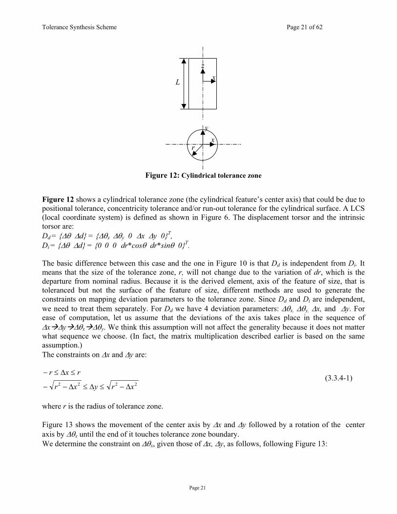
Figure 12: Cylindrical tolerance zone
Figure 12 shows a cylindrical tolerance zone (the cylindrical feature’s center axis) that could be due to positional tolerance, concentricity tolerance and/or run-out tolerance for the cylindrical surface. A LCS (local coordinate system) is defined as shown in Figure 6. The displacement torsor and the intrinsic torsor are: Dd = {∆θ ∆d} = {∆θx ∆θy 0 ∆x ∆y 0}T,
Di = {∆θ ∆d} = {0 0 0 dr*cosθ dr*sinθ 0}T. The basic difference between this case and the one in Figure 10 is that Dd is independent from Di. It means that the size of the tolerance zone, r, will not change due to the variation of dr, which is the departure from nominal radius. Because it is the derived element, axis of the feature of size, that is toleranced but not the surface of the feature of size, different methods are used to generate the constraints on mapping deviation parameters to the tolerance zone. Since Dd and Di are independent, we need to treat them separately. For Dd we have 4 deviation parameters: ∆θx, ∆θy, ∆x, and ∆y. For ease of computation, let us assume that the deviations of the axis takes place in the sequence of ∆x ∆y ∆θx ∆θy. We think this assumption will not affect the generality because it does not matter what sequence we choose. (In fact, the matrix multiplication described earlier is based on the same assumption.) The constraints on ∆x and ∆y are:
2222 xryxr
rxr
∆−≤∆≤∆−−
≤∆≤− (3.3.4-1)
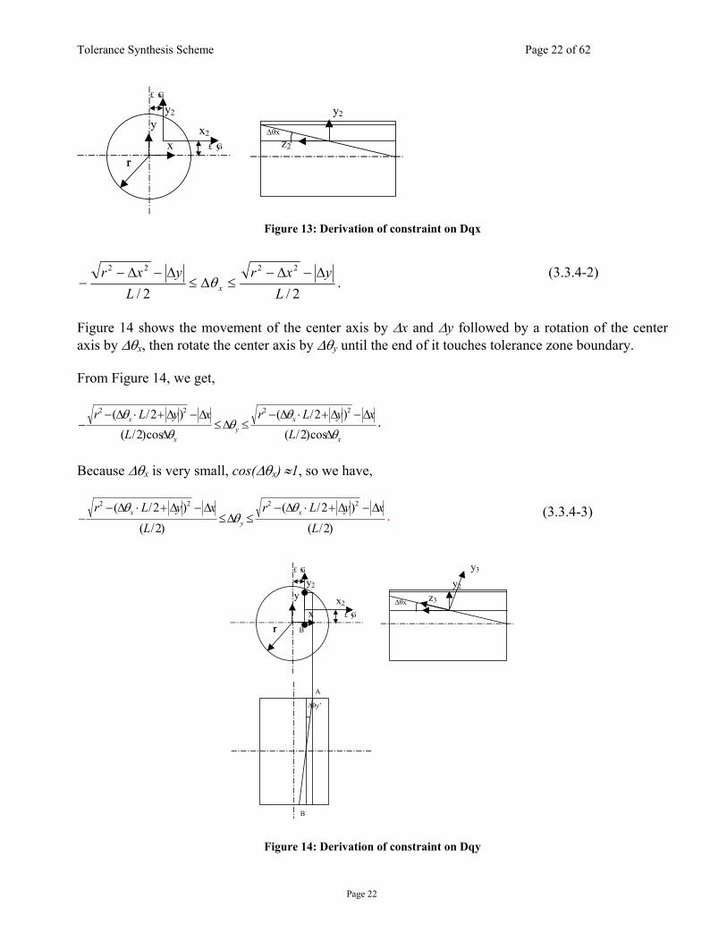
where r is the radius of tolerance zone. Figure 13 shows the movement of the center axis by ∆x and ∆y followed by a rotation of the center axis by ∆θx until the end of it touches tolerance zone boundary. We determine the constraint on ∆θx, given those of ∆x, ∆y, as follows, following Figure 13:
Page 21
Tolerance Synthesis Scheme Page 22 of 62
y
x
y2
x2
£ Gx
£ Gy
r r
y2
z2
∆θx
Figure 13: Derivation of constraint on Dqx
2/2/
2222
Lyxr
Lyxr
x
∆−∆−≤∆≤
∆−∆−− θ .
(3.3.4-2)
Figure 14 shows the movement of the center axis by ∆x and ∆y followed by a rotation of the center axis by ∆θx, then rotate the center axis by ∆θy until the end of it touches tolerance zone boundary. From Figure 14, we get,
x
xy
x
x
LxyLr
LxyLr
θθ
θθ
θ∆
∆−∆+⋅∆−≤∆≤
∆
∆−∆+⋅∆−−
cos)2/()2/(
cos)2/()2/( 2222
.
Because ∆θx is very small, cos(∆θx) ≈1, so we have,
)2/()2/(
)2/()2/( 2222
LxyLr
LxyLr x
yx ∆−∆+⋅∆−
≤∆≤∆−∆+⋅∆−
−θ
θθ . (3.3.4-3)
B
y
x
y2
x2
£ Gx
£ Gy
r r
y2
z3 ∆θx
y3
A
B
∆θy’
Figure 14: Derivation of constraint on Dqy
Page 22

Tolerance Synthesis Scheme Page 23 of 62
Inequalities (3.3.4-1,3.3.4-2,3.3.4-3) are the mapping results for the positional tolerance modified by RFS specified on a cylindrical feature of size.
3.3.5 Spherical Surface A local coordinate system (LCS) is defined for a spherical surface and the deviation parameters are defined in that LCS. For a spherical surface, the LCS is: the z-axis is along a radius of the sphere, and (x, y) are local orthogonal co-ordinates at the center of the sphere (Figure 15, Figure 16). For this surface the deviation parameters of the SDT are: (∆x, ∆y, ∆z, 0, 0, 0 ) and dr. Based on this notation, constraints could be derived connecting these parameters with the specified tolerance values as detailed below.
Figure 15: Spherical feature with LCS
xy
z
TL
Figure 16: Spherical feature with
Page 23
B
A
S Φ TUr ±2
t
olerance specification
Tolerance Synthesis Scheme Page 24 of 62
The VCB of the spherical surface is constructed with the following properties:
o A perfect shape as that of the nominal spherical feature, o A size (diameter) of 2r+TU+Tp, because it is an external feature and the positional tolerance is
modified to MMC, o A perfect location as that of the nominal cylindrical feature.
By applying the same procedures as was followed for the cylindrical case, we have:
Dd = {∆θ ∆d} = {0 0 0 ∆x ∆y ∆z}T, Di = {∆θ ∆d} = {0 0 0 dr*sinφ*cos ψ dr*sinφ*sinψ dr*cosφ}T, and
++∆++∆++∆
=
+++
∆∆∆
1cos)(
sinsin)(cossin)(
1cos)(
sinsin)(cossin)(
1000100010001
ψψφψφ
ψψφψφ
drrzdrrydrrx
drrdrrdrr
zyx
.
The 4 by 4 matrix on the left hand side of the above equation is the transformation matrix for any point on the spherical surface due to displacement torsor assuming the transformation sequence ∆x ∆y ∆z. The 4 by 1 matrix (vector) on the left hand side of the equation represents the changed position of the point due to the intrinsic torsor. The constraint equation is given by:
. and4/)2()cos)(()sinsin)(()cossin)(( 2222
TLdrTPTUrdrrzdrrydrrx
−≥++≤++∆+++∆+++∆ ψψφψφ
We need the above inequality to be valid ∀Φ ∈ (0, 2π) and ∀Ψ ∈ (0, 2π). So we eliminate parameters Φ and Ψ by maximizing the following function.
ψψφψφψφψφ cos2sinsin2cossin2cossin),( 22 zyxaaf ∆+∆+∆++= , where a = r + dr
.0sin2cossin2sinsin2sincos2 0/ , 0)sincossin(cos2 0/
=∆−∆+∆−−⇒=∂∂=∆+∆+⇒=∂∂
ψψφψφψψψψψφφφ
zyxafyxaf
Here, we have two sets of solutions (a symbolic software package was used to get the solutions in symbolic form):
1) )2)2(2(where
, ,2
)12(
2222223242
1
yyazzxazxyzyazazzxyatgn
∆−∆+∆+−∆∆+∆+∆+∆−=∆+∆∆−
−=+= −
β
βψπφ
Page 24

Tolerance Synthesis Scheme Page 25 of 62
2)
).)222()222()2
22()222((where
,)12(,)(
)(sin
22222
3222222442222432
2342244222242
222222
21
222
22222221
xyazzyzazaxzazazxaxyyaxyazyza
xzazazxyyxyaxaa
zayxaxytg
azayxayzayxax
∆∆+∆−∆∆
−∆−∆∆+∆+∆+∆−∆−∆−∆∆−−+∆∆
+∆∆−∆+∆∆+∆+∆+∆+∆−=
∆−∆−∆+−
−∆∆=
∆−∆−∆+−
∆−∆−∆+∆+−∆−= −−
γ
γγγγγψ
γγγγγγγφ
The final set of constraints is:
.
,2
2 2
max
TUdrTL
TpTUrf
≤≤−
++
≤
When the toleranced feature is internal, for example a hole, the final constraint will be:
.
,2
2 2
min
TUdrTL
TpTUrf
≤≤−
−+
≥
If the external feature is modified to LMC, the constraint will be:
.
,2
2 2
min
TUdrTL
TpTLrf
≤≤−
−−
≥
If the internal feature is modified to LMC, the constraint will be:
.
,2
2 2
max
TUdrTL
TpTLrf
≤≤−
+−
≤
3.3.6 Conical Feature
A local coordinate system (LCS) is defined for a conical surface and the deviation parameters are defined in that LCS. For a conical surface, the LCS is: the z-axis is along the cone axis and (x, y) are local orthogonal co-ordinates on the bottom plane of the cone (Figure 17). For this surface the deviation parameters of the SDT are: (∆x, ∆y, ∆z, ∆θx, ∆θy, 0) and dr. Based on this notation, constraints could be derived connecting these parameters with the specified tolerance values as detailed below.
Page 25

Tolerance Synthesis Scheme Page 26 of 62
Figure 17: Coni
R2
R1
L
=
∆∆∆
∆∆
=0θθ
Dzyx
D Iy
x
d
A point P on the nominal surface
rr ,sin,cos θθ
=
−−
++
∆∆∆−∆∆−∆∆
1
sin)(cos)(
10001
1001
1
21
1
RRL
RRrR
drrdrr
zyx
xy
x
yθθ
θθθθ
For the tolerance specification of the following fe
Pag
z
y
xcal feature with LCS
0sincos
000
θθ
drdr
, (3.3.6-1)
−−
LRRrR
21
1 , will transform to:
∆++∆++∆−−−
∆+−−
∆−+
∆+−−
∆++
1
sin)(cos)(
sin)(
cos)(
2
1
21
1
21
1
zdrrdrrLRr
yLRRrR
drr
xLRRrR
drr
xy
x
y
θθθθ
θθ
θθ
(3.3.6-2) ature, the constraints will be:
e 26

Tolerance Synthesis Scheme Page 27 of 62
.sin)(cos)(
,sin)(
,cos)(
where
,
21
1
21
1
21
1
2122
zdrrdrrLRRrRz
yLRRrRdrry
xLRRrRdrrx
TUrzL
RRyxTLr
xy
x
y
∆++∆++∆−−−
=′
∆+−−
∆−+=′
∆+−−
∆++=′
+≤′−
+′+′≤−
θθθθ
θθ
θθ
(3.3.6-3)
We need to find the Max and Min of zL
RRyxrf ′−+′+′= 2122),( θ , to eliminate r and θ. However,
we cannot yet solve the two non-linear equations formed by equating the partial derivatives of the function f with respect to r and t to zero in compact (symbolic) form. So in order to use the results for the conical surfaces in the tolerance synthesis/assemblability analysis, we have to explore further to get a solution or else develop/adopt methods to treat the equation keeping the two free parameters as extra variables.
TUTLr ±2φ
R2 R1
L1
L
Xo
Page 27

Tolerance Synthesis Scheme Page 28 of 62
Figure 18: Conical feature with tolerance specification
3.3.7 Special cases 3.3.7.1 Composite tolerance specification Sometimes we have more than one tolerance specified on one feature of size, as shown in Figure 19. In this case, more constraints need to be generated. A designer has two intents when specifying combined tolerances: 1) both tolerances must be satisfied at the same time, and 2) some DOFs of the feature of size will be constrained specifically by the additional tolerance. In the following case, the perpendicular tolerance gives more constraint on the orientation of the feature of size.
Page 28

Tolerance Synthesis Scheme Page 29 of 62
B
TL
The ASME Y14.satisfied independexample, the consderivation of the c The function of thfeature. Because pthe tolerance onlytolerance can be c
∆∆−−∆
00
1001
θθ xy
Therefore, the con
cos)(( drr ∆++ θ with the constrain
A
Figure 19: Composite tolerance specification
C
5 standard requires that all the tolerances specified to one featuently. This means that we need to treat every tolerance seprattraints for positional tolerance are same as those in Section 3.3.3; onstraints for perpendicular tolerance.
e perpendicular tolerance here is to give more constraints on therpendicular tolerance does not fix the position of virtual condi controls orientation, the position of the transformed point due tan be calculated as follows:
+∆++∆−∆−+∆++
=
++
∆
1sin)(cos)(
sin)(cos)(
1
sin)(cos)(
100100
θθθθθθθ
θθ
θθ
drrdrrzzdrrzdrr
zdrrdrr
xy
x
y
x
y
straint equation will be:
4/()sin)(() 22 2Vxy )TTU2rzdrrz ++≤∆−++ θθθ ,
t equation by positional tolerance:
Page 29
Φ TUr ±2
re of size must be ely. For the above the following is the
e orientation of the tion boundary, and o the perpendicular
θ.
(3.3.7.1-1)
Tolerance Synthesis Scheme Page 30 of 62
4/Tp)TU2r()sin)(()cos)(( 222 ++≤∆+∆−++∆+∆++ yzdrrxzdrr xy θθθθ . (3.3.7.1-2) Equation (3.3.7.1-1) and (3.3.7.1-2) are the constraints due to the composite tolerance specification in the above example. Using the same procedure as in section 3.3.3 to eliminate θ and z, we have thefollowing constraints on deviations for the perpendicular tolerance:
.0,)(1
min
,0,)(1
max
get, we,0 and ,0
zero, tof of sderivative partial theequatingBy . , ,
,)sin()cos(),(
22
2
22
22
min
22
2
22
22
max
22
+
+
+
±
=′
+
+
+
±
=′
=∂′∂
=∂′∂
′
∆−=∆=+=+++=′
bd
abadbdf
bd
abadbdf
zff
dbdrrawheredzabzazf
xy
θ
θθθθθ
From the last section for a positional tolerance of similar specification, we have:
.0,))(1(
min,0,))(1(
max
get, ,0 ,0
zero, tof of sderivative partial theequatingBy
. , , , ,where ,)sin()cos(),(
22
222
22
min22
222
22
max
22
+
+−++
±
=
+
+−++
±
=
=∂∂
=∂∂
∆=∆−=∆=∆=+=+++++=
bd
cdbeabadbdf
bd
cdbeabadbdf
wezfandf
yedxcbdrraedzacbzazf
xy
θ
θθθθθ
The final constraints due to perpendicular tolerance and positional tolerance are:
.
,2
2
,2
2
2
max
2
max
TUdrTL
TvTUrf
TpTUrf
≤≤−
++
≤′
++
≤
(3.3.7.1-3)
Page 30
Tolerance Synthesis Scheme Page 31 of 62
When the toleranced feature is internal, as for example, for a hole, the constraints are:
.
,2
2
,2
2
2
min
2
min
TUdrTL
TvTUrf
TpTUrf
≤≤−
−+
≥′
−+
≥
(3.3.7.1-4)
If the external feature is modified to LMC, the constraints will be:
.
,2
2
,2
2
2
min
2
min
TUdrTL
TvTLrf
TpTLrf
≤≤−
−−
≥′
−−
≥
(3.3.7.1-5)
If the internal feature is modified to LMC, the constraints will be:
.
,2
2
,2
2
2
max
2
max
TUdrTL
TvTLrf
TpTLrf
≤≤−
+−
≤′
+−
≤
(3.3.7.1-6)
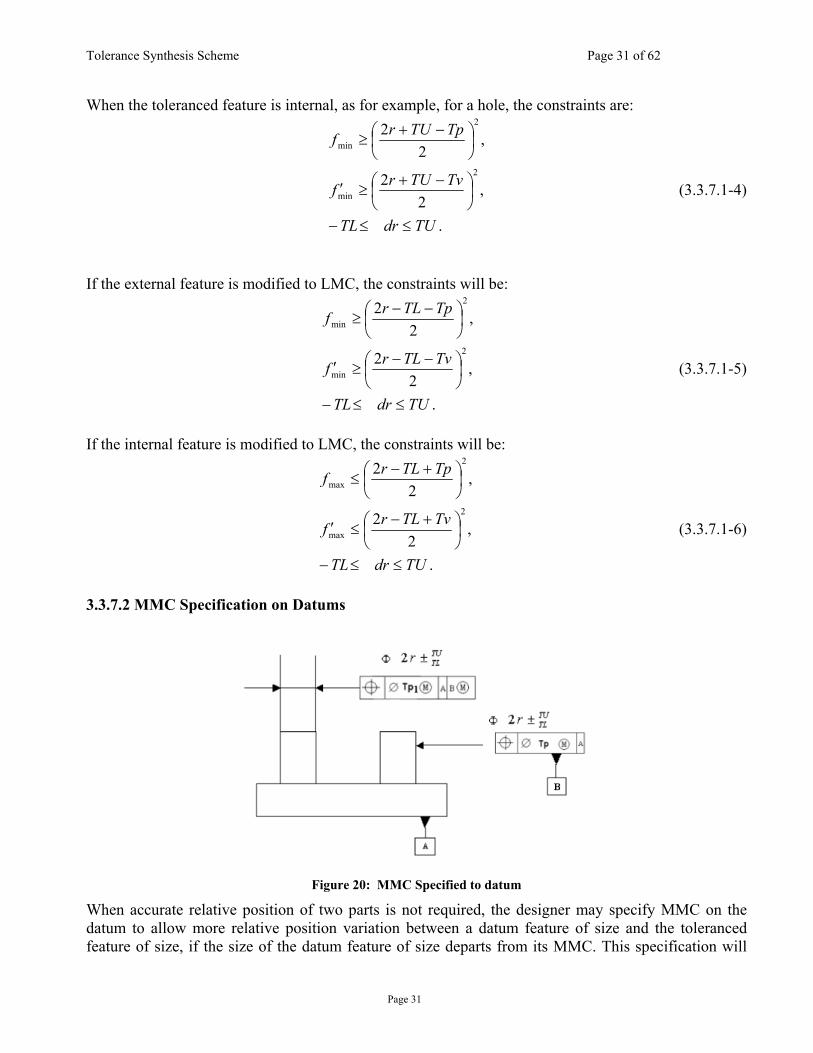
3.3.7.2 MMC Specification on Datums
Figure 20: MMC Specified to datum
When accurate relative position of two parts is not required, the designer may specify MMC on the datum to allow more relative position variation between a datum feature of size and the toleranced feature of size, if the size of the datum feature of size departs from its MMC. This specification will
Page 31

Tolerance Synthesis Scheme Page 32 of 62
not increase the size of the VCB but will allow its center axis to move if the datum feature of size departs from its MMC. In contrast to the composite tolerance specification described in previous section, the position of the VCB of the left hand side cylindrical feature is dependent on the real size of the cylindrical feature on the right hand side. Because this specification means that both cylindrical features will mate features on the other part and the clearance due to the departure of size of datum feature of size from its MMC is allowed to be used to adjust the position of left side cylindrical feature, this problem can be modeled as if we have the positional tolerance and perpendicular tolerance specified on the left-hand feature. The positional tolerance will be Tp1+(TU+Tp-dr) 6 and the perpendicular tolerance is Tp1. Following the procedures as described in Section 3.2, we can develop the constraints on deviations of the left hand side cylindrical feature by substituting Tp= Tp1+(TU+Tp-dr) and Tv=Tp1 :
.
,2
12
2dr)-Tp(TUTp12
2
max
2
max
TUdrTL
TpTUrf
TUrf
≤≤−
++
≤′
++++
≤
Example of Some Mappings
Case 1: Planar Feature
Figure 21: Planar feature (rectangular) with size tolerance
4
x
Figure 21 shows a simple size tolerance to a planar surface with LCS specified. Lhand side surface is the implicit datum and the other side is controlled by the toler
Page 32
6 In this case (TU+Tp-dr) is from the other cylindrical feature
6±0.08
3
zx
et uanc
y
s assume the left e specification.

Tolerance Synthesis Scheme Page 33 of 62
From Figure 21, we know the deviation parameters for the right hand side surface which is a non-size feature are ∆θx, ∆θy, ∆z. The following constraints are established by considering the deviation at the four extreme points (corners) of the plane which are nominally at (1.5, 2, 0), (1.5, -2, 0), (-1.5, 2, 0) and (-1.5, -2, 0).
-0.08 ≤ ∆z + 1.5*∆θy - 2*∆θx ≤ 0.08, -0.08 ≤ ∆z + 1.5*∆θy + 2*∆θx ≤ 0.08,
-0.08 ≤ ∆z – 1.5*∆θy + 2*∆θx ≤ 0.08,
-0.08 ≤ ∆z – 1.5*∆θy - 2*∆θx ≤ 0.08. The above constraints on deviation parameters result in a diamond shape in deviation space as follows:.
Figure 22: Deviation space for size tolerance on planar surface
0.053
-0.08
0.08
-0.053
-0.04
0.04
z
∆θy
∆θx
Page 33

Tolerance Synthesis Scheme Page 34 of 62
Case 2: Cylindrical mating
Figure 23: Assembly of two parts specified with positional tolerance From the above specification, we know that the VCB of the external feature of the above part is equal to that of the internal feature of the bottom part. Following equations (3.3.3-1) and (3.3.3-2), the size of the VCB for the external cylindrical feature is 5+0.25+0.05= 5.3, and that of the internal cylindrical feature is .5.7-0.35-0.05= 5.3. Therefore, we know that the two parts are guaranteed to be assembled. Now let’s see what constraints on deviation parameters we can get by our tolerance mapping, so we can computationally perform the tolerance analysis or synthesis.
.0,)(1
min,0,)(1
max
, , , , ,Let
22
2
22
22
min22
2
22
22
max
+
+−+
+
±
=
+
+−+
+
±
=
∆=∆−=∆=∆=+=
bd
cdbeabadbdf
bd
cdbeabadbdf
yedxcbdrra xy θθ
The final set of constraints for the external feature is:
.25.025.0
,2
05.025.05 2
max
≤≤−
++
≤
dr
f
When the toleranced feature is internal, as for example, for a hole, the constraints are:
.35.035.0
,2
05.035.07.5 2
min
≤≤−
−−
≥
dr
f
Page 34
Tolerance Synthesis Scheme Page 35 of 62
The above equations connot be reduced further in compact form so no further derivation and/or plotting is possible. However, the inequalities as such could be used in computations.
4. Optimization Process Formulation of the Cost Functions The cost function to be minimized can have several components, including:
o Cost of Manufacturing, o Cost of Assembling, o Cost of Inspection, o Cost related to product life span, o Cost to meet functional requirements, o Cost to meet assemblability, etc.
In this study, we have considered the Cost of Manufacturing in details and a new cost of manufacturing model [deviation-based cost of manufacturing] has been introduced. Apart from the cost of manufacturing, we could not yet carry out further investigation into the cost of assembly, inspection, product life-span related costs, etc. Some authors have done context specific work on the above costs and, for example, Dong [DON97] has considered the effect of tolerance on cost related to product lifespan by constructing a functional performance index generated from the effect of tolerance. However, the work is applicable to very specific domains and cannot be used universally. In our tolerance synthesis scheme, we have not considered these costs. In the proposed tolerance synthesis scheme, we have kept a generalized cost of manufacturing model so that the designer can easily introduce/modify the cost functions associated with each part in the artifact library [ROY01]. The cost function has been kept as a virtual function in the artifact class so that the specific cost models could be introduced in the instantiated object from a class of real cost functions. We would consider the last two of the above cost factors (Cost to meet functional requirements and Cost to meet assembleability) as constrains rather than minimization criteria. We will now go into details of cost of manufacturing.
4.1 Cost of Manufacturing We consider the cost associated with manufacturing a part for specified material, dimensions/geometric shape, a sequence of manufacturing operations, and the process capabilities. In general, the cost of manufacturing is a function of all the above entities. Many researchers have analyzed various issues associated with the cost of manufacturing in relation to tolerances and the cost of manufacturing as a decreasing function of a single tolerance parameter. Various functional forms (like the inverse power law, exponential decay, etc.) have been used as cost models that are generally monotonically decreasing functions of increasing in tolerance value. Effect of process capabilities on cost of manufacturing has also been well studied by several authors [DON97].
Page 35

Tolerance Synthesis Scheme Page 36 of 62
Also, since, in general, more than one operation is required to transform the raw blank into the final finished part, the cost of manufacturing is a function of the process sequence and of how much accuracy is achieved in each stages of operation. The cost is also affected by the setup error in each machining process. The total cost of production thus becomes a sum of the costs associated with each process [ROY97]. While none of these methods mentioned above could claim to be universal, there are several limitations with the one-parameter (single tolerance) cost of manufacturing formulation. In reality, a manufactured surface would rarely have a single tolerance value. Apart from a size tolerance, there could be geometric tolerances (form tolerance, orientation tolerance, etc) and it would be difficult to formulate a single parameter representing all these tolerances that could effectively be used for representing the cost of manufacturing. In order to circumvent the above problem, we propose a new formulation for the cost of manufacturing, which we would like to call the deviation-based model.
4.2 Deviation-based Cost Model of Manufacturing In general, a part will have more than one feature, and is connected to other features of other parts and since each feature could possibly have up to six degrees of freedom, the scheme we have adopted uses six deviation parameters to represent the variations associated with each feature. In our earlier reports, we have used the small deviation torsors (SDT) for representing the deviations of features. We have also shown that these deviation parameters are related to the tolerance specifications through a functional mapping (a one to many relation: a tolerance specification defined a bounded region in the deviation space). In our approach, we propose to represent the cost of manufacturing as function of these deviation parameters. Thus, for example, the cost function g(δ) defined as a function of some tolerance value δ, would become a function of the six parameters g(δ) = g( δ(θx θy θz δx δy δz), and then the cost functions could be treated as functions of the small deviation parameters associated with the surface/part. We propose to model the cost of manufacturing a part as an explicit product of six functions of the six deviation parameters in the form:
DCOM(d) = C1(d1)*C2(d2)*….C6(d6) , (4.2-1) where d = (d1, d2, d3, d4, d5, d6) = (θx , θy , θz , δx , δy , δz) is a 6-componenet torsor representing the six deviation parameters characteristic of the feature. The form of the individual functions can vary depending on the specific surfaces and manufacturing process. Some of the functions could be of similar form. Also depending on the nature/type of the feature, some of the functions will be constants (i.e. ∀x, f(x) ≡ 1) and could be eliminated. These functions correspond to the deviation parameters that are invariants of the surface. For an example, for a planar surface there are only three independent parameters given by: d = (dx, 0, 0, 0, θy , θz ) that affect the deviation of the surface from it’s nominal shape; changes in the remaining three keep the surface invariant. The cost function can then be represented as:
Page 36

Tolerance Synthesis Scheme Page 37 of 62
DCOM(d) = Cx(dx)*Cθ(θy)*Cθ(θz). (4.2-2) Also, in this case, since the surface is symmetric about the y and z axes, the form the two functions for rotational deviations along these two directions are also same, namely Cθ. We have mentioned earlier in this section that the deviation parameters are restricted by the tolerance specification. For the planar feature, this mapping forms a convex hull in the form of a diamond in the 3-D space. For a rectangular planar section with cross-section ( ‘a’ x ‘b’), (see section 3.3.2), the following are the constraints: TSL ≤ min (dX + a*θy + b* θz , dX + a*θy - b* θz , dX - a*θy + b* θz , dX - a*θy - b* θz , (4.2-3) TSU ≥ max (dX + a*θy + b* θz , dX + a*θy - b* θz , dX - a*θy + b* θz , dX - a*θy - b* θz ), (4.2-4) where (TSL, TSU) are the lower and upper values of the tolerance parameter for the planar surface. Thus, the parameters dx θy θz are restricted. The cost function (3-2) will be restricted accordingly. To illustrate the cost function, let us assume a generic function of the form: C(x) = a +b/|x|, where x is the deviation parameter and a and b are constants. For the planar case, we then get,
DCOM(d) = Cx(dx)*Cθ(θy)*Cθ(θz)=(a1+b1/|dx|) * (a2+b2/|θy|) * (a3+b3/|θz|)
To further simplify, we assume, a=b=1 and a2 = a3, b2 = b3.
Then we have
-TSL ≤ (dX + θy + θz ) ≤ TSU,
- TSL ≤ (dX + θy - θz) ≤ TSU, -TSL ≤ (dX - θy + θz ) ≤ TSU, - TSL ≤ (dX - θy - θz ) ≤ TSU,
and DCOM(d) = (a1+b1/|dx|) * (a+b/|θy|) * (a+b/|θz|).
Removing the z-parameter θz again so that we can have a visual representation of the cost function, we have - TSL ≤ (d + θ ) ≤ TSU - TSL ≤ (d - θ ) ≤ TSU and
DCOM(d) = (a1+b1/|d|) * (a+b/|θ|). (4.2-5)
In the d-θ plane, this would look like a tent bounded by four vertical planes (by the tolerance specification) approaching infinity along the two axes (Figure 24, Figure 25).
Page 37

Tolerance Synthesis Scheme Page 38 of 62
Figure 24: Cost as function of deviation parameters
Cost
θ
d
- TSL ≤ (d + θ ) ≤ TSU - TSL ≤ (d - θ ) ≤ TSU
d
Cost contours, increasing towards the axes
Figure 25: Co
It is to be noted that the actual form of the inevident that since the deviation parametersfunctions of these deviation parameters shou
θ
st contour lines and the bounds
dividual cost functions are yet to be determined. Also, it is limit the tolerance values in some way or other, the cost ld also be monotone non-increasing in nature.
Page 38

Tolerance Synthesis Scheme Page 39 of 62
4.3 Optimization Process Based on the models described above, the optimization process could be summarized as below: Minimize:
Cost of production: C(x) = Σ(i ∈ all_parts)Σ(j∈ all_mating_features) C(xij), (4.3-1)
where xij is the deviation parameters of the jth feature of part i in the assembly Subject to:
Functional constraints of the form: G(x) ≤ 0, x ∈ Rn , (4.3-2)
Linear Assembliability Constraints of the form: Ax = b , where A = [aij] is an m x n matrix, aij∈ R, x ∈ Rn
, b ∈ Rm , and m is the number of constraints. In general, m is less than the number of variables n.
Deviation to tolerance mapping constraints: FDPk(x) ≤ FTolk(t), x∈Rn, k∈ N+ (4.3-3) where FDP denotes Function of Deviation Parameter, FTol denotes Function of tolerance parameter subscript k is the number of constraint equations. In order to look for a solution for the above minimization formulation that falls under the non-linear programming [NLP] category, we are proposing to develop suitable and efficient evolutionary algorithms [EA] because of the potential problems that could be anticipated in using standard gradient-based NLP solvers as detailed below. The problem formulated above has several layers of complexity that make the problem very difficult to solve using traditional methods. We have tried to formulate the constraints for a very simple, elementary, two dimensional, planar, 3-element assembly [Appendix-A] for which we need about 150+ variables, 80+ linear constraints, 10+ non-linear constraints. We assumed there were no constraints arising out of function requirements and assumed a fairly complex [exponential and inverse] cost function. We then tried to solve the problem using the Matlab NLP solver fmincon. We got some solutions after several trials but the solution is not realistic unless we impose several restrictions on the deviation parameters as well as the tolerance parameters. We anticipate that a medium to reasonably large sized assembly with say a couple of hundred parts in a 3D space would give rise to several thousands of variables and constraints. Apart from that the matrix A in the linear assembleability constraints Ax = b could be very sparse depending upon the assembly, requiring special treatment.
In addition, it is our endeavor to establish a deviation hull as a suitable solution space for further mapping of the tolerance space. This task itself is quite complicated and we believe an approach using the EA techniques could give us some lead by, for example, storing the intermediate solutions and doing some analysis of the pattern. However, this area is open for further research.
Page 39

Tolerance Synthesis Scheme Page 40 of 62
Computer Implementation of the Tolerance Synthesis System The proposed tolerance synthesis system has been considered as an object-oriented representation built in part on our earlier work [ROY01] where we introduced a generic artifact class that can be extended to include a tolerance class and other class structures. We developed the class structures using UML (Rational Rose 2000 - Enterprise Edition). We plan to do the full-scale implementation in C++ and add interfaces with 3D CAD packages such as AutoCAD, ProE, and SolidWorks etc, so that the end user could interact with a user-friendly graphic environment for defining the product and carry out the desired tolerance related computations. At present the graphics display and other graphics driven design/tolerance synthesis aspects are being formulated for use with SolidWorks. Appendix – B shows a part of the class diagrams of the basic entities in the synthesis scheme. A very skeletal (but operational) tolerance synthesis method has been implemented under the Windows environment as a core module without Windows GUI and CAD interfaces using a database programming system (Clipper 5.2). In order to make manipulation of the model data easy, systematic, and structured, the entire data associated with each model is stored in a relational database system with several tables for each type of object/class. The structures of these tables, along with relational links between the tables, have been shown in Appendix–C. The field names in each table have been kept nearer to their real counterparts for ease of understanding. The program is menu driven and operates in two phases. In the first phase, the designer would build the model (artifact) using standard artifact library elements and specifying other details. After a model has been established, governing equations for each independent path are generated and then the equations are converted into a set of MatLab input files for optimization. Cost functions and constraints for the functional requirements are formulated separately as MatLab input files. MatLab is then used to solve the resulting nonlinear optimization problem for arriving at a set of optimal deviation parameters. Details of the Example Model In Appendix – D we present details of an example model including part/feature details, input data listing, generated data (partial list), generated MatLab input files (mostly generated from the synthesis module), and some preliminary results. It has already been mentioned that we are using MatLab to solve the cost minimization problem. In the present case, only a sample (fictitious) cost function has been used to test if the constraints generated could be properly treated in MatLab. The optimized output results are of little significance here since those are based on fictitious cost functions. We are now in the process of selecting realistic cost functions and various models, so that some practical tolerance limits/bounds could be computed based on the optimization results.
Acknowledgement This work is sponsored by the SIMA (Systems Integration for Manufacturing Applications) program at NIST and the RaDEO (Rapid Design Exploration and Optimization) program at DARPA. The authors also wish thank the reviewers for their valuable comments and suggestions.
Page 40

Tolerance Synthesis Scheme Page 41 of 62
Disclaimer No approval or endorsement of any commercial product by the National Institute of Standards and Technology is intended or implied. Certain commercial equipments, instruments, or materials are identified in this report in order to facilitate better understanding. Such identification does not imply recommendations or endorsement by the National Institute of Standards and Technology, nor does it imply the materials or equipment identified are necessarily the best available for the purpose.
References [BAL00] E. Ballot, P. Bourdet, A Mathematical Model of Geometric Errors in the case of
Specification and 3D Control of Mechanical Parts. Advanced Mathematical and Computational Tools in Metrology IV, 2000 World Scientific Publishing
[BAL98] E. Ballot, P. Bourdet, A Computation Method for the Consequences of Geometric Errors in
Mechanisms. Geometric Design Tolerancing: Theories, Standards, and Applications, Hoda A. Elmaraghy (Editor), Chapman & Hall, pp 197-207, 1998.
[DAS97] D. Dasgupta, Z. Michalewicz, Evolutionary Algorithms in Engineering
Applications,Springer-Verlag, 1997, ISBN: 3-540-62021-4 [DON97] Zuomin Dong, Tolerance Synthesis by Manufacturing Cost Modeling and Design
Optimization, Advanced Tolerancing Techniques, Edited by Hong-Chao Zhang, John Wiley & Sons, Inc, pp 233-260, 1997.
[DRA99] Drake, Paul, Dimensioning and Tolerancing Handbook, McGraw-Hill, 1999 [GIL91] Gilbert, Olivier L., Representation of Geometric Variations Using Matrix Transforms for Statistical Tolerance Analysis in Assemblies, Master thesis, MIT, 1992
[LIN97] Shui-Shun Lin, Hsu-Pin (Ben) Wang and Chun (Chuc) Zhang, Optimal Tolerance Design
for Integrated Design, Manufacturing, and Inspection with Genetic Algorithms, Advanced Tolerancing Techniques, Hong-Chao Zhang (Editor), John Wiley & Sons, Inc, pp 261-281, 1997.
[MAT98] L. Mathieu, A. Clement and P. Bourdet, Modeling, Representation and Processing of
Tolerances, Tolerance Inspection: A Survey of Current Hypothesis. Geometric Design Tolerancing: Theories, Standards, and Applications, Hoda A. Elmaraghy (Editor), Chapman & Hall, pp 1-33, 1998.
[ROY97] Utpal Roy and Ying-Che Fang, Optimal Tolerance Re-allocation for the Generative
Process Sequence, IIE Transactions, Vol 29, pp 37-44, 1997. [ROY99] U Roy, Bing Li. Representation and interpretation of geometric tolerances for polyhedral
objects-II. Size, orientation and position tolerances. Computer-Aided Design 31 (1999), pp 273-285.
Page 41
Tolerance Synthesis Scheme Page 42 of 62
[ROY00a] U. Roy, Bing Li, Tolerance Synthesis by Manufacturing Cost Modeling and Design
Optimization, Advanced Tolerancing Techniques, Edited by Hong-Chao Zhang, John Wiley & Sons, Inc, pp 233-260, 1997.
[ROY00b] U. Roy, N. Pramanik, Tolerance Representation and Synthesis Scheme Interim Report # 4:
Submitted to NIST, March 2000. [ROY00c] U. Roy, N. Pramanik, System Level Tolerancing: Standards and Implementation Issues:
Tolerance Representation and Synthesis Scheme Interim Report # 6: Submitted to NIST, July 2000.
[ROY00d] U. Roy, N. Pramanik, System Level Tolerancing: Standards and Implementation Issues:
Tolerance Representation and Synthesis Scheme Interim Report #7: Submitted to NIST, September 2000.
[ROY00e] U. Roy, N. Pramanik, and H. Wang System Level Tolerancing: Standards and
Implementation Issues: Tolerance Representation and Synthesis Scheme Interim Report #8: Submitted to NIST, March 2001.
[ROY01] U. Roy, N. Pramanik, R. Sudarsan, R. D. Sriram and K. W. Lyons, Function-to-Form
Mapping: Model, Representation and Applications in Design Synthesis, Journal of Computer-Aided Design (accepted for publication).
[ROY02] Utpal Roy, and Balaji Bharadwaj. Design with Part Behaviors: Behavior Model,
Representation and Application. Journal of Computer-Aided Design (in press).
Page 42

Tolerance Synthesis Scheme Page 43 of 62
Appendix – A: An Example of Deriving Assembliability
Constraints Mathematical Model of Tolerances
Various mathematical models for representation of components in an assembly have been studied so that the geometric variations arising out of small deviations of the features (faces) of the components could be analyzed. We adopted the small displacement torsor scheme to represent the deviation of a real surface with respect to the corresponding nominal surface at a point on a feature/face of a component. Based on this scheme, an effective representation of kinematic variations for the mating faces/features could be formulated as elaborated hereinafter. A torsor is a tensor-type representation of small displacements and rotations (corresponding to the six degrees of freedom associated with a space point on a surface embedded in R3). If we introduce three small displacements along the three local principal axes at a point A on a surface as δ = [δx δy δz]T and three rotations θ = [θx θy θz ]T then the torsor TA/R at A with reference to a datum R can be represented as:
TA/R = [θA δA ]T = [θx θy θz δx δy δz ]T.
Torsors transform according to standard rotation and translation rules of axes. However, the components are small in comparison to the dimension of the components. The torsor representation of deviations of real surfaces with respect to the nominal surface for all possible regular surface geometries used in engineering design have been well studied. It has been found that, there can be some component (out of the possible six) variations along which the surface is kept invariant with respect to the nominal surface. These components are called independent components and may be varied for considering possible configurations. As for example, for a cylindrical surface, a translation along the axis keeps the surface invariant as does a o a rotation about the axis. Thus the torsor representation for the deviation is:
y x
z
TA/R = [θA δA ]T = [Rx θy θz Ix δy δz ]T
Page 43

Tolerance Synthesis Scheme Page 44 of 62
where I stands for independent movement (in this case along the axis of the cylinder) and R stands for free rotation (here, about the axis of the cylinder). We can arbitrarily make these quantities zero so that they do not enter into the equations. In addition, we can vary these parameters for various constraint satisfactions keeping the surfaces invariant. The small-displacement torsor mentioned above could be used to represent three types of deviations associated with the mating of components in an assembly. Two torsors associated with each component and a gap torsor at the mating. The two torsors associated with each surface are: a displacement torsor and a deviation torsor as shown in Figure 26. The displacement torsor is an intrinsic variation torsor that is specific to the element (as for example, displacement arising out of the variation of the radius of a cylindrical surface). The displacement torsor represents the deviation of the real surface from the nominal surface. The gap torsor between two mating features represents possible geometric variations between the mating features, as depicted in Figure 26.
Figure 26: Interacting torsors at mating surfaces
Gap
Displacement Nominal
Part B
Part A Real Surface
Deviation torsor
Deviation torsor
Displacement
The torsor scheme indicated above could be used to form equations based on loops connecting components in an assembly. Torsors associated with each component feature would be kept in the artifact library in the local coordinate system of the component. The gap torsor associated with two mating features would be formed based the functional and/or kinematic requirements as established in the design specifications. In order to add the torsors in a loop to form equations connecting the components of the torsors, a mechanism would be necessary to transform the torsors defined in the
Page 44

Tolerance Synthesis Scheme Page 45 of 62
local coordinate systems of the individual components into a global reference frame. Since a torsor is represented by a 1x6 vector, the transformations required would be 6x6 transformation matrices. Torsor Transformation Rules The small displacement torsor TN = [θN δN ]T = [θx θy θz δx δy δz ]T defined at a point N on a surface could be expressed at a point M on a different surface by applying the required displacement and rotation to the vector MN. The transformation is a 6x6 matrix given by:
∆∆−∆−∆∆∆−
=
100001000010000100000010000001
xyxz
yzD ,
where (∆x ∆y ∆z)T is the vector from M to N. The transformation is given by TM = DTN and it can be explicitly written as
.
)()()(
×+=
∆−∆+∆−∆+∆−∆+
=
NN
N
xyz
zxy
yzx
z
y
x
M
MN
yxxzzy
Tθδ
θ
θθδθθδθθδ
θθθ
The torsor scheme for the modeling of the small geometric variations of connecting features/faces of an artifact has been elaborated with a simple example of a rectangular block (Part-3) enclosed within two channels (Part-1 and Part-2) (Figure 27, Figure 28). Apart from the simplified configuration, further simplification has been done as detailed below so that the relevant transformations and preliminary computations could be checked manually.
Page 45

Tolerance Synthesis Scheme Page 46 of 62
Figure 27: Example problem with three blocks
Part -
Loop –1 Part -
Loop –2
Loop –3 Part - Loop –4
Loop –5
Loop –6
Part -
Part -
y y z x 22 23 24 21 25 33 y 32 z 34 31
11 15 12 y 14 y 13 x
Figure 28: Example problem with feature numbers and LCS
Part -
The simplifications are:
a) All variations take place along the vertical plane only (with 3 possible variations: x-rotation, y-displacement and z-displacement) to keep the formulation simple.
Page 46
Tolerance Synthesis Scheme Page 47 of 62
b) There is no displacement torsor for each part. Only the surface deviation torsors and
the gaps are taken into consideration.
c) The bottom surface of Part 1 has been assumed to be a fixed datum. The three parts 1, 2, and 3, local axes and contact surfaces have been shown in the same sketch. Surfaces have been designated as <part_number><serial_number> such that surfaces on part 1 are numbered as 11, 12, 13, 14, etc. For generating equations connecting the variations of the mating surfaces, six loops have been considered (Figure 27). With the above simplifications, we are left with following configuration: Number of mating surfaces : 14 (all planer) Number of gaps between mating surfaces : 8 Number of surface parameters : 14 x 3 = 42 Number of gap parameters : 8 x 3 = 24 Total number of parameters : 42 + 24 = 66 Number of loops : 6 Number of equations from the loops : 6 x 3 = 18 The six loops are as follows:
Loop-1: 12 32 31 13 Loop-2: 11 21 22 32 32 12 Loop-3: 22 32 33 23 Loop-4: 24 34 33 23 Loop-5: 15 25 24 34 34 14 Loop-6: 14 34 31 13
The associated torsors in their local coordinate systems are: T11 , T12, T13, T14, T15, T21, T22, T23, T24, T25, T31, T32, T33, T34. Typically, each of these torsors would have similar 6-component forms like: T11 = [θ11 δ11 ]T = [θx11 0 0 0 δy11 δz11 ]T , T12 = [θ12 δ12 ]T = [θx12 0 0 0 δy12 δz12 ]T. The gap torsors are: G11/21, G12/32, G13/31, G14/34, G15/25, G22/32, G23/33, G24/34, with typical forms given by: G11/21 = [θg11/21 δg11/21 ]T = [θgx11/21 0 0 0 δgy11/21 δgz11/21 ]T.
Page 47

Tolerance Synthesis Scheme Page 48 of 62
We now consider the Loop - 1 (12 32 31 13) and write the torsor equation for the loop as:
T12 + G12/32 + (-T32 ) + T31 + (-G13/31 ) + (-T13 ) = 0. Transforming all the terms in the above equation in Part–1’s frame of reference, the equation becomes, T12
+ (D12/23)12 G12/32 + (D32)12 (-T32 ) +(D31)12 T31 +(D13/31)12 G13/31 + (D13)12 (-T13 ) = 0, where the D’s are the corresponding transformations with respect to the Part - 1. Writing the D’s in full, and carrying out the operations, the above equation becomes,
[θx12 0 0 0 δy12 δz12 ]T + [θgx12/32 0 0 0 δgy12/32 δgz12/32 ]T - [θx32 0 0 0 δy32 + θx32 (z32 - z12) δz32 + θx32 (y32 - y12) ]T + [θx31 0 0 0 δy31 + θx31 (z31 - z12) δz31 + θx31 (y31 - y12) ]T + [θgx13/31 0 0 0 δgy13/31 + θgx13/31 (z31 - z12) δgz13/31 + θgx13/31 (y31 - y12)]T - [θx13 0 0 0 δy13 + θx13 (z13 - z12) δz13 + θx13 (y12 - y12)]T
= [ 0 0 0 0 0 0 ]T
. Equating each component to zero gives six scalar equations. In this present case, there are only three equations due to the restricted space of the example.
θx12 + θgx12/32 - θx32 + θx31 + θgx13/31 - θx13 = 0,
δy12 + δgy12/32 - δy32 - θx32 (z32 - z12) + δy31 + θx31 (z31 - z12) + δgy13/31 + θgx13/31 (z31 - z12) - δy13 + θx13 (z13 - z12) = 0,
δz12 + δgz12/32 - δz32 - θx32 (y32 - y12) + δz31 + θx31 (y31 - y12) + δgz13/31 + θgx13/31 (y31 - y12) - δz13 + θx13 (y12 - y12) = 0.
Each of the six loops will give three similar equations. Altogether eighteen equations would be formed connecting the sixty-six parameters. Let us repeat the procedure of forming the equations for Loop–2 (11 21 22 32 32 12). The torsor equation for the Loop - 2 is: T11 + G11/21 + (-T21 ) + T22 + (G22/32 ) + (-T32 ) + T32 + (G32/12 ) + (-T12 ) = 0, i.e., T11 + G11/21 + (-T21 ) + T22 + (G22/32 ) + (G32/12 ) + (-T12 ) = 0.
Page 48

Tolerance Synthesis Scheme Page 49 of 62
Transforming all the terms in the above equation in Part–1’s frame of reference, the equation becomes, T11
+ (D11/21)11 G11/21 + (D21)11 (-T21 ) +(D22)11 T22 +(D22/32)11 G22/32 + + (D32/12)11 G22/12 + (D12)11 (-T12 ) = 0, where the D’s are the corresponding transformations with respect to the Part-1. Writing the D’s in full, and carrying out the operations, the above equation becomes,
[θx11 0 0 0 δy11 δz11 ]T + [θgx11/21 0 0 0 δgy11/21 δgz11/21 ]T - [θx21 0 0 0 δy21 + θx21 (z21 - z11) δz21 + θx21 (y21 - y11) ]T + [θx22 0 0 0 δy22 + θx22 (z22 - z11) δz22 + θx22 (y22 - y11) ]T + [θgx22/32 0 0 0 δgy22/32 + θgx22/32 (z22 - z11) δgz22/32 + θgx22/32 (y22 - y11)]T + [θgx32/12 0 0 0 δgy32/12 + θgx32/12 (z32 - z11) δgz32/12 + θgx32/12 (y32 - y11)]T - [θx12 0 0 0 δy12 + θx12 (z12 - z11) δz12 + θx12 (y12 - y11)]T
= [ 0 0 0 0 0 0 ]T
. Equating each component to zero gives following three equations:
θx11 + θgx11/21 - θx21 + θx22 + θgx22/32 + θgx32/12 - θx12 = 0,
δy11 + δgy11/21 - δy21 - θx21 (z21 - z11) + δy22 + θx22 (z22 - z11) + δgy22/32 + + θgx22/32 (z22 - z11) +δgy32/12 + θgx32/12 (z32 - z11) - δy12 - θx12 (z12 - z11) = 0,
δz11 + δgz11/21 - δz21 - θx21 (y21 - y11) + δz22 + θx22 (y22 - y11) + δgz22/32 + θgx22/32 (y22 - y11) + δgz32/12 + θgx32/12 (y32 - y11) - δz12 - θx12 (y12 - y11) = 0.
Similar procedures would yield the rest of the equations for the remaining four loops. The gap parameters have to be generated / constrained based on the physical nature of mating between the pair of surfaces and/or design functional requirements. Converting a functional requirement into some constraint binding the gap parameters is a very complex task and currently not many generalized treatments have been published (as far as knowledge of this author goes). However, many people are carrying out work for this goal. In our present work, we have assumed that the mapping from functional requirements to constraints binding the gap parameters have been carried out, and the corresponding constraint equations have been obtained.
Page 49

Tolerance Synthesis Scheme Page 50 of 62
Appendix – B: Class diagrams of the basic entities in the synthesis scheme
Page 50
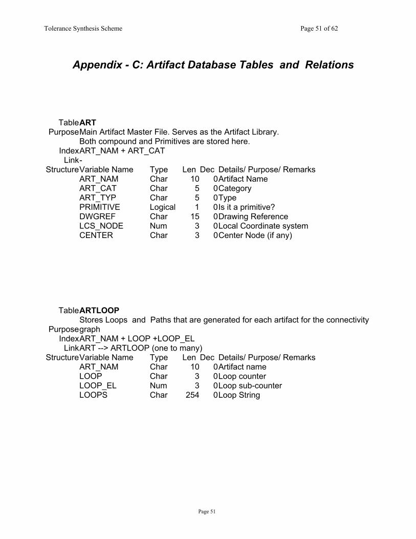
Tolerance Synthesis Scheme Page 51 of 62
Appendix - C: Artifact Database Tables and Relations
Table ART Purpose Main Artifact Master File. Serves as the Artifact Library. Both compound and Primitives are stored here. Index ART_NAM + ART_CAT Link - Structure Variable Name Type Len Dec Details/ Purpose/ Remarks ART_NAM Char 10 0Artifact Name ART_CAT Char 5 0Category ART_TYP Char 5 0Type PRIMITIVE Logical 1 0Is it a primitive? DWGREF Char 15 0Drawing Reference LCS_NODE Num 3 0Local Coordinate system CENTER Char 3 0Center Node (if any)
Table ARTLOOP
Purpose Stores Loops and Paths that are generated for each artifact for the connectivity graph
Index ART_NAM + LOOP +LOOP_EL Link ART --> ARTLOOP (one to many) Structure Variable Name Type Len Dec Details/ Purpose/ Remarks ART_NAM Char 10 0Artifact name LOOP Char 3 0Loop counter LOOP_EL Num 3 0Loop sub-counter LOOPS Char 254 0Loop String
Page 51
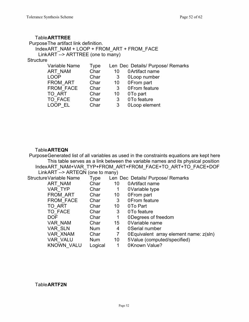
Tolerance Synthesis Scheme Page 52 of 62
Table ARTTREE Purpose The artifact link definition. Index ART_NAM + LOOP + FROM_ART + FROM_FACE Link ART --> ARTTREE (one to many) Structure Variable Name Type Len Dec Details/ Purpose/ Remarks ART_NAM Char 10 0Artifact name LOOP Char 3 0Loop number FROM_ART Char 10 0From part FROM_FACE Char 3 0From feature TO_ART Char 10 0To part TO_FACE Char 3 0To feature LOOP_EL Char 3 0Loop element Table ARTEQN Purpose Generated list of all variables as used in the constraints equations are kept here This table serves as a link between the variable names and its physical position IndexART_NAM+VAR_TYP+FROM_ART+FROM_FACE+TO_ART+TO_FACE+DOF Link ART --> ARTEQN (one to many) Structure Variable Name Type Len Dec Details/ Purpose/ Remarks ART_NAM Char 10 0Artifact name VAR_TYP Char 1 0Variable type FROM_ART Char 10 0From part FROM_FACE Char 3 0From feature TO_ART Char 10 0To Part TO_FACE Char 3 0To feature DOF Char 1 0Degrees of freedom VAR_NAM Char 15 0Variable name VAR_SLN Num 4 0Serial number VAR_XNAM Char 7 0Equivalent array element name: z(sln) VAR_VALU Num 10 5Value (computed/specified) KNOWN_VALU Logical 1 0Known Value?
Table ARTF2N
Page 52
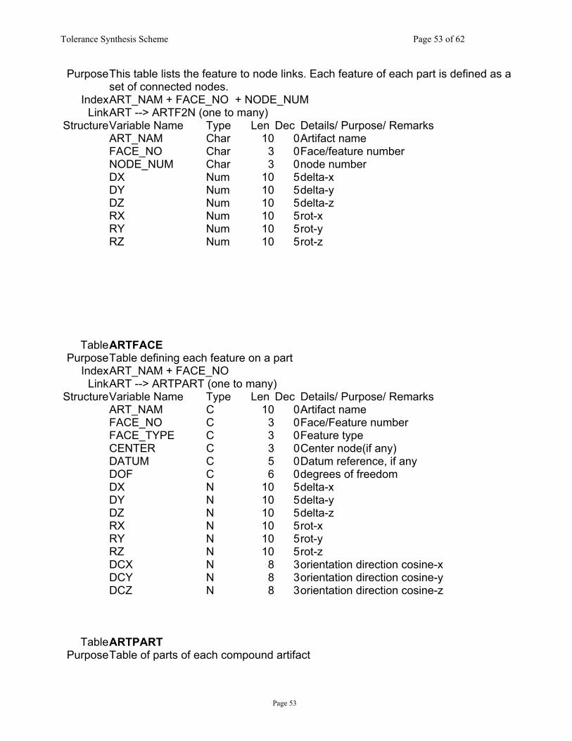
Tolerance Synthesis Scheme Page 53 of 62
Purpose This table lists the feature to node links. Each feature of each part is defined as a set of connected nodes. Index ART_NAM + FACE_NO + NODE_NUM Link ART --> ARTF2N (one to many) Structure Variable Name Type Len Dec Details/ Purpose/ Remarks ART_NAM Char 10 0Artifact name FACE_NO Char 3 0Face/feature number NODE_NUM Char 3 0node number DX Num 10 5delta-x DY Num 10 5delta-y DZ Num 10 5delta-z RX Num 10 5rot-x RY Num 10 5rot-y RZ Num 10 5rot-z Table ARTFACE Purpose Table defining each feature on a part Index ART_NAM + FACE_NO Link ART --> ARTPART (one to many) Structure Variable Name Type Len Dec Details/ Purpose/ Remarks ART_NAM C 10 0Artifact name FACE_NO C 3 0Face/Feature number FACE_TYPE C 3 0Feature type CENTER C 3 0Center node(if any) DATUM C 5 0Datum reference, if any DOF C 6 0degrees of freedom DX N 10 5delta-x DY N 10 5delta-y DZ N 10 5delta-z RX N 10 5rot-x RY N 10 5rot-y RZ N 10 5rot-z DCX N 8 3orientation direction cosine-x DCY N 8 3orientation direction cosine-y DCZ N 8 3orientation direction cosine-z Table ARTPART Purpose Table of parts of each compound artifact
Page 53
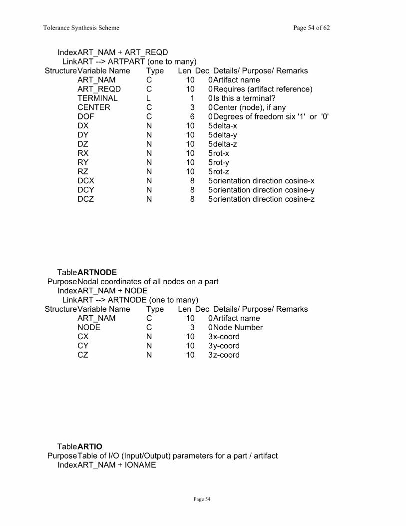
Tolerance Synthesis Scheme Page 54 of 62
Index ART_NAM + ART_REQD Link ART --> ARTPART (one to many) Structure Variable Name Type Len Dec Details/ Purpose/ Remarks ART_NAM C 10 0Artifact name ART_REQD C 10 0Requires (artifact reference) TERMINAL L 1 0Is this a terminal? CENTER C 3 0Center (node), if any DOF C 6 0Degrees of freedom six '1' or '0' DX N 10 5delta-x DY N 10 5delta-y DZ N 10 5delta-z RX N 10 5rot-x RY N 10 5rot-y RZ N 10 5rot-z DCX N 8 5orientation direction cosine-x DCY N 8 5orientation direction cosine-y DCZ N 8 5orientation direction cosine-z
Table ARTNODE Purpose Nodal coordinates of all nodes on a part Index ART_NAM + NODE Link ART --> ARTNODE (one to many) Structure Variable Name Type Len Dec Details/ Purpose/ Remarks ART_NAM C 10 0Artifact name NODE C 3 0Node Number CX N 10 3x-coord CY N 10 3y-coord CZ N 10 3z-coord
Table ARTIO Purpose Table of I/O (Input/Output) parameters for a part / artifact Index ART_NAM + IONAME
Page 54

Tolerance Synthesis Scheme Page 55 of 62
Link ART --> ARTNODE (one to many) Structure Variable Name Type Len Dec Details/ Purpose/ Remarks ART_NAM C 10 0Artifact name IOTYPE C 5 0I/O Type IONAME C 10 0I/O Name IOCAT C 5 0Category IOUNIT C 5 0Unit IOVALU N 10 3Value
Page 55

Tolerance Synthesis Scheme Page 56 of 62
Appendix – D: Tolerance Synthesis Example Model In this section we present preliminary results for an example artifact with three blocks (consisting of parts 1, 2, 3) as shown in Figure 29. This artifact as represented in the program is shown along with local coordinate systems for each feature in Figure 30. The program first generates the artifact tree from the input configuration (Figure 31) and then all independent paths/loops are generated in an exhaustive manner (Figure 32). Each path/loop is used to generate assemblability constraints. As has been shown earlier these assemblability constraints are in the form KX = b. For ease of handling these constraints in Matlab, a sparse matrix representation has been used for the K-matrix. This implementation has a built-in procedure to generate cost functions based on deviation parameters. The cost function generated for this example is shown in Figure 33. For solving the optimization (minimization) problem as formulated in this program, we are using “fmincon”, a nonlinear constrained optimization facility in Matlab. The program generates a “dot m file” for running the optimization in Matlab. Results of the optimization run are depicted in Figure 34 as a distorted shape of the original (nominal) artifact shown in Figure 30. These deviation parameters signify the amount permissible variations of each critical feature of the assembly within the prescribed ranges of assembly and functional constraints. In order to arrive at a specific tolerance specification we need to carry out following steps:
o Identify candidate features for tolerancing, o Determine datum reference frames (DRF), o Decide tolerance types, o Generate Tolerance Specification from Deviation to Tolerance Mappings for the corresponding features.
This work is in progress and we will report actual mapping to a particular tolerance specification in our next NIST IR.
Figure 29: Block Artifact
Page 56

Tolerance Synthesis Scheme Page 57 of 62
Figure 30: Nominal shape with local coordinate systems (LCS)
Figure 31: Feature to feature connectivity diagram
Page 57

Tolerance Synthesis Scheme Page 58 of 62
Figure 32: Artifact Control main Screen
Figure 33: Sample cost of Manufacturing Function
Page 58
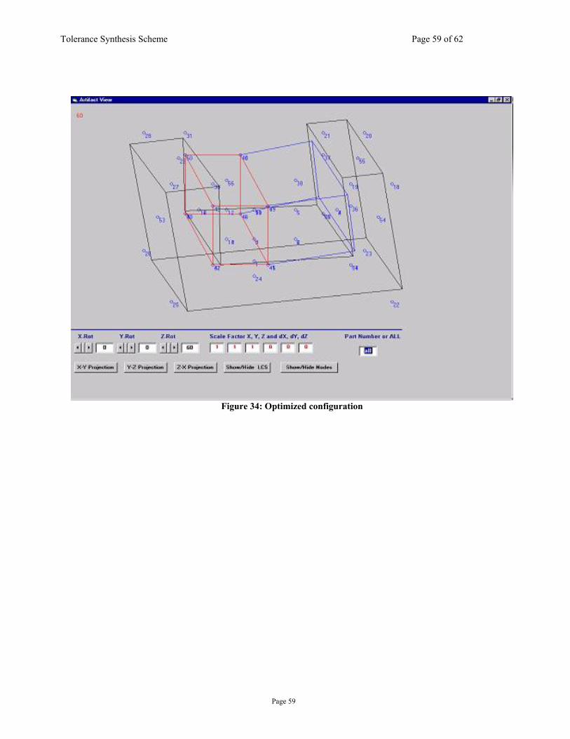
Tolerance Synthesis Scheme Page 59 of 62
Page 59
Figure 34: Optimized configuration


![Pituitary Lesions, Obesity, and Mesenteric Lipomas in ... · insulin sensitivity via the insulin-modified, frequently-sampled intravenous glucose tolerance test (FSIGTT) [5]. ...](https://static.fdocuments.net/doc/165x107/602099004fee671578648e12/pituitary-lesions-obesity-and-mesenteric-lipomas-in-insulin-sensitivity-via.jpg)


