Research & Development

Tolerable Variation in Item

Parameter Estimates for

Linear and Adaptive

Computer-based Testing

July 2004 RR-04-28

ResearchReport

Saba Rizavi

Walter D. Way

Tim Davey

Erin Herbert

Tolerable Variation in Item Parameter Estimates for Linear and Adaptive

Computer-based Testing

Saba Rizavi, Walter D. Way, Tim Davey, and Erin Herbert

ETS, Princeton, NJ

July 2004

ETS Research Reports provide preliminary and limiteddissemination of ETS research prior to publication. Toobtain a PDF or a print copy of a report, please visit:

www.ets.org/research/contact.html

Abstract

Item parameter estimates vary for a variety of reasons, including estimation error, characteristics

of the examinee samples, and context effects (e.g., item location effects, section location effects,

etc.). Although we expect variation based on theory, there is reason to believe that observed

variation in item parameter estimates exceeds what theory would predict. This study examined

both items that were administered linearly in a fixed order each time that they were used and

items that had appeared in different adaptive testing item pools. The study looked at both the

magnitude of variation in the item parameter estimates and the impact of this variation in the

estimation of test-taker scores. The results showed that the linearly administered items exhibited

remarkably small variation in parameter estimates over repeated calibrations. Similar findings

with adaptively administered items in another high stakes testing program were also found when

initial adaptively based item parameter estimates were compared with estimates from repeated

use. The results of this study also indicated that context effects played a more significant role in

adaptive item parameters when the comparisons were made to the parameters that were initially

obtained from linear paper-and-pencil testing.

Key words: Item parameter estimates, computer adaptive testing, IRT, scoring

i

Acknowledgements

The authors would like to express their gratitude to Dr. Valerie Folk for reviewing this paper,

and to Diane Cruz and Roxanna Paez for their help and cooperation during this project.

ii

Computer-based testing, and adaptive testing in particular, typically depends upon item

response theory (IRT). The advantages of IRT are well-known through the testing literature and

have fueled the transition of computerized adaptive testing (CAT) from a research interest to a

widely used practical application. However, the introduction of computer-based testing in high

volume, high stakes settings has presented new challenges to testing practitioners. In most

computer-based testing programs, it is necessary to administer items repeatedly over time. This

continuous item exposure raises security concerns that were not fully appreciated by researchers

when the theory and practice of CAT were first developed.

In most CAT programs, steps are taken to protect the integrity of item pools through

strategies such as item exposure control, pool rotation, and accelerated item development (Way,

1998). Despite such efforts, maintaining CAT programs remains difficult because adaptive

algorithms tend to select the most highly discriminating items. Efforts to increase item

development bring increased costs and diminishing returns. As these items become exposed and

are retired from use, developing sufficient replacement items of the same quality is very difficult:

Three or four items may need to be written to find a suitable replacement. Furthermore, the lag

time between the initial writing of the items and use of the items in an operational CAT pool is

usually significant, as items must be pretested, calibrated, and evaluated before they may be used

operationally.

Recently, researchers at ETS have begun exploring an approach to adaptive testing that

could address some of the challenges of item exposure and pool maintenance (Bejar et al., 2002).

Bejar (1991) referred to this approach as generative testing. More recently it has been called item

modeling. The essence of item modeling is to create items from explicit and principled rules. The

approach has roots in computer-assisted instruction and domain-referenced testing (Hively,

1974). The obvious vehicle for item modeling is the computer, and successful applications of

automated item generation have been reported by a number of researchers (Embretson, 1999;

Irvine, Dunn, & Anderson, 1990; Irvine & Kyllonen, 2001).

Although the capability to develop item models and generate items automatically is more

easily established for some item types than for others, the potential utility of automated item

generation for supporting computer-based testing is obvious. An effective item model provides

the basis for a limitless number of items, each of which is assumed to share the same content and

statistical characteristics. In CAT, the adaptive algorithm could choose an item model based on

1

the common psychometric characteristics, and the actual instance of the item would be generated

at the time of delivery. Such an approach was referred to as on-the-fly adaptive testing by Bejar

et al. (2002). They carried out a feasibility study of a CAT application where item models were

utilized and concluded that the adaptive generative model they employed was both technically

feasible and cost effective.

From a traditional IRT perspective, the use of item models with adaptive testing seems

far-fetched. In fact, much of the IRT literature in recent years has centered on item parameter

estimation and parameter recovery, the idea being that successful applications of IRT depend

upon well-estimated parameters. The notion that one could use a single set of IRT estimates to

characterize all of the items generated from a particular model directly contradicts the goal of

obtaining accurate item parameter estimates. However, such a perspective does not account for

the variation that may occur in student scores due to a variety of effects that influence how test

items are responded to in the real world. These include context effects, item position effects,

instructional effects, variable sample sizes, and other sources of item parameter drift that are

typically not formally recognized or controlled for in the context of CAT.

Several researchers have documented the existence and influence of such item level

effects. Sireci (1991) looked at the effect of sample sizes on the stability of IRT item parameter

estimates. Kingston and Dorans (1984) described such effects in equating the paper-and-pencil

GRE. Leary and Dorans (1985) and Brennan (1992) reviewed literature related to context effects

and provided guidelines on how such effects might be minimized. Zwick (1991) described a case

study of how context effects created an anomaly in the Reading test scores on the National

Assessment of Educational Progress (NAEP). Divgi (1986) documented changes in item

parameter estimates in an early application of the Armed Services Vocational Aptitude Battery

(CAT-ASVAB). Several researchers have investigated causes of item parameter drift in testing

programs that utilized IRT in test construction and equating over time (Eignor & Stocking, 1986;

Kolen & Harris, 1990; Sykes & Fitzpatrick, 1992; Way, Carey, & Golub-Smith, 1992).

In considering the viability of item models for CAT, we recognize that variation within

models introduces a source of errors that is not present in traditional CAT. However, the

repeated use of the same items across different CAT pools also introduces a source of errors that

is tolerated but not accounted for. The purpose of this study was to investigate and to quantify

the error that is currently tolerated in item parameter estimates for different sets of items used in

2

computer-based testing. The study examined items that were administered repeatedly to different

examinee samples over time. We examined items that, each time they were used, were

administered linearly in a fixed order and also items that had appeared in different adaptive

testing item pools. We examined both the magnitude of variation in the item parameter estimates

and the impact of this variation on the test takers’ scaled or reported scores.

Case Study 1: Linear Administration of Items

Data

In order to carry out the investigation of the stability of parameter estimates in linearly

administered tests, two sets of items from a high stakes admissions test were chosen. The first set

was composed of 28 items from the Quantitative (QNT) measure, while the second set consisted

of 30 items from the Verbal (VBL) measure of the same test. Since ability distributions for the

Quantitative measure are known to change more rapidly than the other measures, a greater

variation in the parameter estimates was expected for that measure.

The items contained in the two sets come from actual test administrations in which these

items were used as anchors to place parameter estimates on the base scale for other items in the

linearly administered pretest sections. In every online pretest calibration for these CAT

programs, anchor items are administered as similarly as possible to pretest items. The

composition of the anchor set mirrors the pretests in terms of psychometric and content

characteristics; the number of items in the pretest and anchor set is the same. The Verbal and

Quantitative anchor items evaluated in the study were used over a 2-year period and were

calibrated for each administration of the corresponding pretest measure. Thus nine repeated

calibrations were available for each anchor item. The average item parameter estimates for both

Quantitative and Verbal measures are presented in Table 1.

The calibration samples were randomly obtained by spiraling the pretest forms across

examinees. The sample sizes used to calibrate each item varied from 627 to 2,305 for the

Quantitative measure and 830 to 2,284 for the Verbal measure. The details of sample sizes used

for each calibration are presented in Table A1. The perfect response patterns were excluded from

each of the response sets; the resulting sample sizes are presented in the last column of that table.

3

Table 1

Average Item Parameter Estimates (a, b)

Calibration a-parameter b-parameter Mean St. dev Mean St. dev

QNT 1 0.842 0.342 –0.020 1.1632 0.852 0.348 –0.008 1.145 3 0.826 0.340 –0.028 1.166 4 0.764 0.365 –0.042 1.341 5 0.764 0.297 –0.030 1.256 6 0.779 0.272 0.016 1.208 7 0.818 0.339 –0.047 1.235 8 0.755 0.335 –0.182 1.305 9 0.775 0.299 –0.036 1.175

VBL

1 1.003 0.292 –0.090 1.150 2 0.983 0.290 –0.034 1.205 3 0.954 0.279 –0.065 1.222 4 0.967 0.270 0.035 1.229 5 1.024 0.291 0.045 1.124 6 1.129 0.313 0.046 1.059 7 0.970 0.278 –0.010 1.114 8 1.020 0.301 0.010 1.107 9 0.954 0.275 –0.061 1.186

Parameter Estimation Methodology

The item parameter estimates were obtained using the software LOGIST (Wingersky,

Patrick, & Lord, 1988). LOGIST uses the joint maximum likelihood estimation methodology to

estimate item parameters, keeping the ability parameters fixed, while formulating item parameter

estimates. The ability parameters in this case were the actual ability estimates obtained on the

operational section of the test. The estimates on the linearly administered items were then

subjected to scaling using the test characteristic curve methodology proposed by Stocking and

Lord (1983). In this study, the stability of estimates on both sets of anchor items was investigated

after the scaling was carried out.

4

Analyses

In order to look at the general trends in the variation of individual parameter estimates the

a, b, and c parameters were plotted for each item across calibrations. The purpose of this analysis

was simply to get an idea of any directional change that could occur in some items over time. In

order to look at the effect of parameter estimate variation on the probability of getting an item

correct, the item characteristic curves were examined for each item across nine calibrations for

both measures. The weighted Root Mean Squared Errors (RMSE) were then computed between

the item characteristic curves for the various calibrations in relation to the first calibration. In

other words the first calibration was chosen as a point of reference for all comparisons in this

case. The RMSE in this case is defined as

n

21

1

( ( ) ( ))jic ic j i jj

RMSE w P Pθ θ=

= −∑ , (1)

where )( jicP θ is the probability of getting an item (i) correct in a calibration (c) at an ability level

jθ . The weight wj is the proportion of examinees out of the total number of examinees and n is

the number of ability levels. The ability levels (and the corresponding weights) were derived

from the reference paper-and-pencil (P & P) base form ability distribution for this particular

program on the number-right scale. The number-right score levels ranged from 10 to 59 for

Quantitative and 15 to 75 for Verbal resulting in 11 and 13 ability levels for the two measures

respectively. The levels were then converted on to the theta metric as listed in Table 2. These

ability levels ranged from –3.839 to 3.546 for Quantitative and –5.855 to 4.881 for Verbal.

This index was used in similar research performed at ETS where the item characteristic

curves (ICCs) obtained on different calibrations were compared (Guo, Stone, & Cruz, 2001;

Rizavi & Guo, 2002). The RMSEs were then plotted for each item across calibrations to capture

variation for items.

5

Table 2

Ability Levels and Corresponding Weights for Quantitative and Verbal Measures

Quantitative Verbal

Level Ability Weight Ability Weight 1 –3.839 0.001 –5.855 0.000 2 –2.184 0.029 –3.355 0.006 3 –1.381 0.100 –2.337 0.019 4 –0.812 0.158 –1.635 0.049 5 –0.348 0.172 –1.074 0.111 6 0.053 0.155 –0.585 0.175 7 0.427 0.125 –0.127 0.195 8 0.807 0.106 0.329 0.163 9 1.242 0.094 0.800 0.130 10 1.882 0.055 1.298 0.084 11 3.546 0.003 1.856 0.051 12 2.608 0.017 13 4.881 0.000

Another interesting way to look at the variation is to estimate the variance-covariance

matrix of item parameter estimates. Several alternatives are available for computing the sampling

variances of item parameter estimates. The first is to use standard large-sample theory, which

holds that the asymptotic variances of < cba ,, > are given by the inverse of the 3 x 3 Fisher

information (I) matrix evaluated at the true parameter values <a, b, c> (Lord, 1980; Hambleton,

Swaminathan, & Rogers, 1991) defined as,

a ab ac

bc

bc

.

i ab b

ac c

I I I

I I I

I I I

Σ =

(2)

The diagonal elements of the matrix represent the information associated with each

parameter. The problem, of course, is that the true parameters are unknown. Our best

approximation is then to evaluate information at the values of the parameter estimates < cba ,, >

and hope that these are reasonably close to the true values. The estimates were averaged across

6

nine calibrations to obtain the best estimate for each item. It is, however, true that the

item parameter estimates are often constrained to avoid taking on inappropriate values (e.g.,

negative a-parameters or c-parameters outside the range [0, 1]). Such constraints are liable to

upset asymptotic theory and render the sampling variance approximations less valid.

In the current situation, a second means is available for estimating sampling variation.

The items under study were administered on nine separate occasions, and parameter estimates

were separately obtained from each administration sample. The observed variation across these

estimates is therefore an empirical estimate of the sampling fluctuation of the parameter

estimates defined as,

=Σ

2bc

bc2

acab2a

cac

babi

σσσ

σσσ

σσσ

. (3)

In theory, and under all of the assumptions of that theory, the empirical and asymptotic

estimates of sampling variation should be very similar. However, the empirical variances are

only based on nine observations and may not be very stable. Both asymptotic and empirical

sampling variance estimates are therefore problematic to some extent. It was therefore decided to

repeat the analyses with both.

The last and the most affirming set of analyses was performed to look at the effect of

variation in the item parameter estimates on the actual reported scores. The responses of

examinees on the anchor items were selected for the nine sets of calibrations on both measures.

A typical ability distribution for the examinees during an administration is given in Figure A5 for

both Quantitative and Verbal. Each response set was then scored using the set of item parameter

estimates obtained on it during calibration process and then using the parameter estimates

obtained using each of the other eight sets of responses. Hence 9 sets of scores were obtained

from each response set. A grand total of 81 sets of scores were produced from the total of 9

response sets. The scoring was carried out using maximum likelihood estimation methodology

(Lord, 1980; Hambleton et al., 1991). RMSE statistics between each set of the baseline theta

estimates (or scores obtained using the set of item parameter estimates obtained on the same

7

response set during calibration process) and the estimates from each of the other eight sets were

then computed. The statistic was defined as,

2

1

ˆ ˆ( ),

kncj kj

ck

j k

RMSEn

θ θ

=

−= ∑ (4)

where is the ability estimate obtained for an examinee j on examinee set (or response set) k

using item parameter estimates obtained by calibrating response set k. On the other hand, is

the ability estimate for an examinee j on examinee set k, using item parameter estimates obtained

by calibrating response set c.

kjθ̂

cjθ̂

The ability estimates were then mapped on to the reported score scale and the

distributions of differences (Scorecj - Scorekj) for each of the 81 scenarios were plotted. The

differences were expressed on the operational or reported score scale where the reported scores

for this particular program are expressed in 10-point intervals.

Case Study 2: Adaptive Administration of Items

Estimation Methodology

The second part of this investigation was carried out on a set of adaptively administered

operational items from another high stakes admissions test. This particular program uses the item

specific prior methodology with a proprietary version of computer software PARSCALE

(Muraki & Bock, 1999). This methodology allows unique multivariate normal distributions to be

used as prior distributions for the parameters of each item (Swaminathan & Gifford, 1986; Folk

& Golub-Smith, 1996). These item specific priors are actually the mean estimates of the (b, a, c)

parameters as well as the asymptotic variance-covariance matrix specified as (Intercept, a, c).

These priors are used for the CAT operational items and are different for each item, as they are

item specific. On the other hand, global priors are used for the pretest items and are the same for

all pretest as well as anchor items. The global prior distributions for the a-parameter are

approximated by lognormal distribution, b-parameter distributions are approximated by normal,

and the c-parameter prior distributions are approximated by beta distribution. All pretest, anchor,

and CAT items are calibrated together for an administration. In this case, pretest or anchor items

8

are actually embedded in the operational test. This is unlike the previous case, where a pretest or

anchor set is offered as a separate section. Since the priors on the CAT items are strong, their

values hardly move away from their original values. The CAT items, therefore, set the scale;

thus, putting all items on the same scale. Once calibrated, the pretest item parameter estimates

are stored in the item bank to be used in subsequent pools, while the operational item parameter

estimates are not used further. This methodology has been shown to be effective in utilizing data

from operational items that do not have a uniform distribution of ability, since they are

administered adaptively.

Data

The data for this investigation came from the Quantitative measure of an adaptively

administered high stakes admissions test. Items that had already appeared in operational pools

and had been included in several pretest calibrations to hold the scale (with item specific priors

on them) were identified. In order to obtain relatively uniform ability distributions, 30 items that

were slightly easy, mid-difficulty, or adequately difficult and had sample sizes larger than 500

associated with them were chosen. The item parameter estimates for these items were originally

obtained when they were pretested in P & P administrations before the introduction of CAT. The

mean and standard deviations for the original a, b, and c parameters are give in Table 3.

Table 3

Mean and Standard Deviations for the a, b, and c Parameters (Original P & P)

a b c

Mean 1.07 0.23 0.16

Stdev 0.19 0.72 0.05

All chosen items had appeared in several pools and had been included in at least 8

calibrations. The number of calibrations available on these items is given in Table 4.

The ability distributions of examinees who received these items in each calibration were

inspected to make sure that the range of examinee abilities for each of these items was not

restrictive. For the purpose of this investigation, all calibrations were rerun with the following

modification: the item specific priors were removed and global priors were imposed on these

9

CAT items, thus they were treated like other pretest items. The modified requests for the

calibration were resubmitted using ETS-specific software called GENASYS, which uses

PARSCALE for calibration. Items were then calibrated in this modified way and new parameter

estimates were obtained.

Table 4

Number of Calibrations

No. of items No. of calibrations 5 8 12 9 7 10 6 11

Analyses

Similar to the previous case study, the item characteristic curves were examined for each

item. The weighted RMSEs were then computed between the ICCs for the first calibration,

compared with the other calibrations as discussed in the previous study. The first calibration was

arbitrarily chosen as the point of comparison.

The next part of the analyses involved looking at the effect of variation in parameter

estimates on ability estimation. Unlike the linear case, where a fixed number of calibrations were

available on each item, the number of calibrations varied in this case (as shown in Table 5, the

number of calibrations on various items varied from 8 to 11). Thus, 20 sets of item parameter

estimates were generated for each item by drawing parameters at random from the various

calibrations available for that item (except the first calibration). A response set was obtained by

generating responses for 1,000 examinees at 11 ability levels corresponding to the ability levels

listed in Table 5. These ability levels are obtained on the number-right scale from the reference P

& P base form. The number-right score for this particular test ranged from 0 to 60, resulting in

11 ability levels with a 6-point interval. The ability levels when converted on to the theta metric

ranged from –3.138 to 2.592.

The item parameter estimates used to generate the response set came from the first

calibration and were considered as the baseline estimates. The response set was scored using

10

baseline parameter estimates from the first calibration, as well as using the 20 other randomly

chosen sets of estimates.

Table 5

Ability levels and corresponding weights for Quantitative CAT

Level Ability Weight 1 –3.138 0.007 2 –1.970 0.057 3 –1.289 0.107 4 –0.772 0.145 5 –0.337 0.163 6 0.054 0.154 7 0.426 0.135 8 0.800 0.110 9 1.210 0.077 10 1.725 0.039 11 2.592 0.005

The first set of scores was then compared to the other 20 sets of scores. RMSEs were

computed between the various sets of ability estimates at each ability level. Since rectangular

distribution was simulated, the mean sum-of-squares at various ability levels were weighted in

order to compute the overall RMSE. The ability estimates were then converted to scaled or

reported scores and the distributions of differences between those scores obtained using various

sets of estimates were compared. The differences were expressed on the operational or reported

score scale where the reported scores for this particular program are expressed in 1-point

intervals.

Next, the scoring analyses were repeated by generating response data using the item bank

parameters for these items. As mentioned earlier, these parameters were originally obtained from

P & P pretest calibrations. These analyses were expected to reveal more variation in scores due

to P & P context effects in addition to positional effects obtained from adaptive administrations.

In real calibrations, these estimates are used as priors for the corresponding items; hence, it is

important to know whether such context effects influence the parameter estimation. The response

set was then scored using the same set of item parameter estimates as well as the remaining 20

sets of estimates.

11

Results

The results of the analyses on linearly administered items are presented first, followed by

the adaptively administered items.

Results for Case Study 1

It should be noted that, for the sake of brevity and clarity, results for Quantitative and

Verbal are presented and discussed side-by-side; however, the authors do not intend to compare

the two measures. Figure 1 presents the test characteristic curves (TCC) for the set of anchor

items for the two measures.

TCC for anchor items for 9 Quantitative packages

0

5 10

15 20 25 30

-3 -2 -1 0 1 2 3

Ability

Sum

of i

tem

pro

babi

litie

s

1

2

3

4

5

6

7

8

9

TCC for anchor items for 9 Verbal packages

0

5

10

15

20

25

30

-3 -2 -1 0 1 2 3Ability

Sum

of i

tem

pro

babi

litie

s 1

2

3

4

5

6

7

8

9

Figure 1. TCC for Quantitative and Verbal anchor items over nine calibrations.

The TCCs for both measures were extremely close under both scenarios. Some variations

at the tails of the curve are characteristic of the interaction between the abilities of examinees and

difficulty level of the items. Those variations are also shown in the plots of ICCs presented in

Figures A1 and A2 in Appendix A. The plots of ICCs for selected Quantitative and Verbal items

show that the probabilities of getting an item right did not vary substantially across calibrations,

except at the very extreme ends of the scale. The investigation of the general trends did not

exhibit any directional change in the estimates. In other words, none of the items exhibited a

systematic decrease or increase in the parameter estimates over repeated calibrations.

12

The RMSEs among ICCs for the two measures are shown in Figure 2. The actual values of

the weighted RMSEs are presented in Tables A2 and A3. The RMSEs indicated a small variation

between calibrations for both Quantitative and Verbal measures. The differences were slightly

higher for Quantitative, especially for some of the items. An item with a very high difficulty level

is what appeared to be the most variant in the Quantitative measure. Inspecting the sample sizes

and ability distribution for that particular calibration of that item did not suggest any explanation

beyond chance-level differences in responding for examinees at extreme ability levels.

MSE

ed R

ight

Weighted RMSEs between VBL ICCs (1st vs. other calibrations)

0.00

0.05

0.10

0.15

0.20

0.25

0.30

2 3 4 5 6 7 8 9

Calibrations

We

s

Weighted RMSEs between QNT(1st vs. other calibrations)

0.00

0.05

0.10

0.15

0.20

0.25

0.30

2 3 4 5 6 7 8 9

Calibrations

Wei

ghte

d R

MSE

s

Figure 2. Weighted RMSEs between ICCs between first calibration and the others.

In comparing the model-based vs. empirical variation (see Figures A3 and A4), it was

found that the model-based variation was larger than the empirical variation for both

Quantitative and Verbal measures for the b-parameter. The model-based variance was highly

affected by the magnitude of the b-parameter: very low b-parameters resulted in large values of

model-based variance. In the case of the a-parameter, model-based variance was larger than the

empirical variation for the Quantitative measure while smaller for the Verbal measure. The a-

parameters for Verbal were, in general, higher in magnitude.

13

In general, the results did indicate very small model-based and empirical variation in both

a- and b-parameters, except for the model-based variance in b-parameter for Quantitative. As

these items provide very little information, the extremely low b-parameters for some of the

Quantitative items caused this variance. In general, these results should be interpreted with

caution, as the samples for the analyses were not suitably sized.

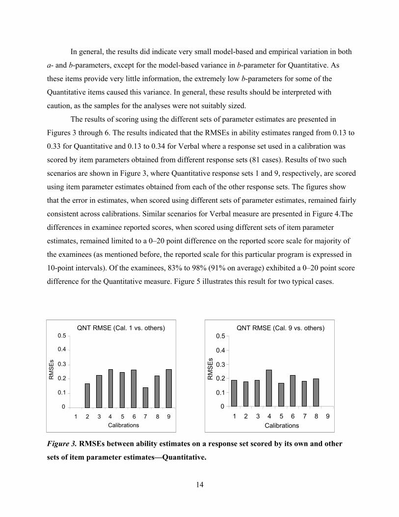
The results of scoring using the different sets of parameter estimates are presented in

Figures 3 through 6. The results indicated that the RMSEs in ability estimates ranged from 0.13 to

0.33 for Quantitative and 0.13 to 0.34 for Verbal where a response set used in a calibration was

scored by item parameters obtained from different response sets (81 cases). Results of two such

scenarios are shown in Figure 3, where Quantitative response sets 1 and 9, respectively, are scored

using item parameter estimates obtained from each of the other response sets. The figures show

that the error in estimates, when scored using different sets of parameter estimates, remained fairly

consistent across calibrations. Similar scenarios for Verbal measure are presented in Figure 4.The

differences in examinee reported scores, when scored using different sets of item parameter

estimates, remained limited to a 0–20 point difference on the reported score scale for majority of

the examinees (as mentioned before, the reported scale for this particular program is expressed in

10-point intervals). Of the examinees, 83% to 98% (91% on average) exhibited a 0–20 point score

difference for the Quantitative measure. Figure 5 illustrates this result for two typical cases.

QNT RMSE (Cal. 1 vs. others)

0

0.1

0.2

0.3

0.4

0.5

1 2 3 4 5 6 7 8 9Calibrations

RM

SEs

QNT RMSE (Cal. 9 vs. others)

0

0.1

0.2

0.3

0.4

0.5

1 2 3 4 5 6 7 8 9Calibrations

RM

SEs

Figure 3. RMSEs between ability estimates on a response set scored by its own and other

sets of item parameter estimates—Quantitative.

14

SE

VBL RMSE (cal. 9 vs. others)

0

0.1

0.2

0.3

0.4

0.5

1 2 3 4 5 6 7 8 9Calibrations

RMSE

s

VBL RMSE (cal. 1 vs. others)

0

0.1

0.2

0.3

0.4

0.5

1 2 3 4 5 6 7 8 9Calibrations

RMs

Figure 4. RMSEs between ability estimates on a response set scored by its own and other

sets of item parameter estimates—Verbal.

The first part of the figure shows response set 2 scored using item parameter estimates

obtained on response set 1. The second part shows response set 9 scored using item parameter

estimates obtained on response set 5. In the first scenario, 93% of the examinees exhibited a 0–

20 point difference in their reported scores, while 90% showed this difference for the second

scenario. Similar results for Verbal are shown in Figure 6. The percentages of examinees

exhibiting 0–20 point score differences ranged from 87% to 98% (94% on average) for Verbal.

Percentage of differences in the reported scores (cal 2, cal 1)

0

10

20

30

40

50

60

0 10 20 30 >30

Difference in scores

Perc

enta

ge o

f exa

min

ees

Percentage of differences in the reported scores (cal 9, cal 5)

0

10

20

30

40

50

60

0 10 20 30 >30

Difference in scores

Perc

enta

ge o

f exa

min

ees

Figure 5. Frequency distribution of reported score differences for Quantitative.

15

Percentage of differences in the

reported scores (cal 2, cal 1)

0

10

20

30

40

50

60

0 10 20 30 >30

Difference in scores

Perc

enta

ge o

f exa

min

ees

Percentage of differences in the

reported scores (cal 9, cal 5)

0

10

20

30

40

50

60

0 10 20 30 >30

Difference in scores

Perc

enta

ge o

f exa

min

ees

Figure 6. Frequency distribution of reported score differences for Verbal.

Since the average Standard Error of Measurement (SEM) ranges from 35 to 45 points for

the Quantitative measure and 30 to 40 points for the Verbal measure of this particular program,

the results were promising for both measures.

Results for Case Study 2

The ICC plots for selected adaptively administered items are presented in Figure B1 in

Appendix B. The weighted RMSEs between ICCs for the adaptive calibrations in comparison with

first adaptive calibration are presented in Figure 7. These values are also presented in Tables B1

and B2 for readers’ interest. The RMSEs among ICCs for those items revealed remarkably small

variation. The values remained in the range of 0.01 and 0.20 for all items for all calibrations.

When compared with scores based on first calibration, the differences in reported scores

for the adaptive case, ranged from 0 to 2 points for 90% to 98% (96% on average) of examinees

for 20 item parameter sets that were drawn from calibrations. At this point it is worth mentioning

again that the reported score scale for this particular program is expressed in 1-point intervals.

The consistency of the RMSEs in the ability estimates across 20 item parameter sets

drawn from available calibrations is depicted in Figure 8. When investigated per ability level

(Figure 9), a large portion of the error seemed to concentrate in the low ability levels.

16

Weighted RMSEs for QNT ICCs

(CAT---1st vs. other calibrations)

0.00

0.05

0.10

0.15

0.20

0.25

0.30

1 2 3 4 5 6 7 8 9 10

Calibrations

Wei

ghte

d R

MSE

s

Figure 7. Weighted RMSEs between CAT ICCs between first calibration and the others.

Weighted RMSEs between scores

(1st calibration set vs. 20 sets)

0

0.1

0.2

0.3

0.4

0.5

1 2 3 4 5 6 7 8 9 10 11 12 13 14 1516 17 18 19 20

Item parameter sets

Wei

ghte

d R

MSE

s

Figure 8. Weighted RMSEs between ability estimates on a response set scored by its own

and another set of item parameter estimates—own set = 1st calibration.

17

Weighted RMSEs between scores

(1st vs. another set)--by ability levels

0

0.2

0.4

0.6

0.8

1

1 2 3 4 5 6 7 8 9 10 11Ability

Wei

ghte

d R

MSE

s

Figure 9. Weighted RMSEs between ability estimates on a response set scored by its own

and another set of item parameters by ability level—own set = 1st calibration.

Percentage of differences in the reported scores

(1st calibration set vs. another set)

0

10

20

30

40

50

60

0 1 2 3 >3

Difference in scores

Perc

enta

ge o

f exa

min

ees

Figure 10. Frequency distribution of reported score differences—comparison with 1st CBT

calibration.

18

When P & P calibrated estimates of the items were used in place of the first calibration

for comparison between calibrations, the results were quite different. Figure 11 shows the

RMSEs between theta estimates obtained on the P & P calibrated sets of parameter estimates and

20 sets of estimates obtained on CBT calibrations. The results indicate an increase of overall

RMSEs, when abilities obtained using P & P estimates were used for comparison. While the

scenario where comparisons were based on 1st calibration and the overall RMSEs between

scores ranged from 0.12 to 0.20, the errors ranged from 0.19 to 0.30 here. The errors in the

scores remained significantly small at the middle ability levels, higher for the high ability levels,

and highest for the low ability levels, when compared across ability levels. The errors were as

high as 0.63 at the lower ability levels.

Weighted RMSEs between scores

(bank parameter set vs. 20 sets)

0

0.1

0.2

0.3

0.4

0.5

1 2 3 4 5 6 7 8 9 10 11 12 13 14 15 16 17 18 19 20

Item parameter sets

Wei

ghte

d R

MSE

s

Figure 11. RMSEs between ability estimates on a response set scored by its own and other

sets of item parameter estimates—own set = P & P bank parameters.

The percentage of examinees that exhibited reported score differences between 0–2

points on the reported score scale ranged from 87% to 94% (91% on average). This percentage

was considerably smaller than the previous scenario where most of the cases resulted in more

than 93% of the examinees exhibiting a 0–2 point difference. In other words, the percentage of

examinees whose scores changed by more than 2 points was significantly large in this case.

19

Weighted RMSEs between scores

(bank parameter set vs. another set)

0

0.2

0.4

0.6

0.8

1

1 2 3 4 5 6 7 8 9 10 11

Ability

Wei

ghte

d R

MSE

s

Figure 12. Weighted RMSEs between ability estimates on a response set scored by its own

and another set of item parameters by ability level—own set = P & P bank parameters.

Percentage of differences in the reported scores

(bank parameter set vs. another set)

0

10

20

30

40

50

60

0 1 2 3 >3

Difference in scores

Perc

enta

ge o

f exa

min

ees

Figure 13. Frequency distribution of reported score differences—comparison with P & P

calibrated parameters.

20

The SEM for the Quantitative measure of this program usually ranges from 2.5 to 3.5

points. In the first scenario, 96% of people exhibiting less than or equal to a 2-point difference

represented an encouraging result. In other words, 4% of the examinees exhibited a difference of

three-or-more points in their reported scores. For the second scenario, where bank parameters were

used to score the responses, 9% of the examinees showed a difference of three-or-more points.

Conclusions

The studies discussed in this paper investigated the effect of stability of item parameter

estimation in the current CBT calibrations. The results of the study will serve as a baseline for

the design work involved in creating models for automated item generation. The concept of

having a single model to generate a family of items should be informed by knowing the relative

stability of the parameter estimates when calibrated online.

Several conclusions can be drawn from the results of this study. The linearly

administered items in a high stakes testing program exhibited remarkably small variation in

parameter estimates over repeated calibrations. Although the sample sizes upon which the

calibrations were performed varied considerably, the results were not affected. As long as the

sample sizes are large enough to calibrate, stable results are produced. Similar findings with

adaptively administered items in another high stakes testing program were also found when

initial adaptively based item parameter estimates were compared with estimates from repeated

use. These findings have implications for research on item modeling because they suggest that

the use of item modeling with operational CAT programs will introduce more variation in ability

estimation due to item context effects, positional effects, and the small sample sizes obtained for

some items. It will be important to quantify and account for these sources of variation as this

research progresses.

The results of this study also indicate that context effects played a more significant role in

adaptive item parameters when the comparisons were made to the parameters that were obtained

from P & P testing. Even though PARSCALE was used to calibrate both sets of items, however,

P & P items went through concurrent calibrations as opposed to item-specific prior methodology

used for adaptive items; this fact may also have caused some variation. This suggests that the

parameter estimates obtained on P & P administrations should be replaced,

21

whenever feasible, with the CBT calibrated parameters. The approach employed for this paper

(i.e., freeing the item specific priors that constrain item parameter estimates for selected

operational items during the process of pretest item calibration) is one possible alternative for

this kind of updating. However, further research would be necessary to determine if this

approach would be feasible in the context of an ongoing, operational CAT program.

22

References

Bejar, I. I. (1991). A generative approach to psychological and educational measurement. (ETS

RR-91-20). Princeton, NJ: ETS.

Bejar, I. I., Lawless, R. R., Morley, M. E., Wagner, M. E., Bennett, R. E., & Revuelta, J. (2002).

A feasibility study of on-the-fly adaptive testing (GRE Board Pro. Rep. No. 98–12; ETS

RR-02-23). Princeton, NJ: ETS.

Brennan, R. (1992). The context of context effects. Applied Measurement in Education, 5, 225–

264.

Divgi, D. R. (1986). Determining the sensitivity of CST-ASVAB scores to changes in item

response curves with the medium of administration. Alexandria, VA: Center for Naval

Analyses.

Eignor, D. R., & Stocking, M. (1986). An investigation of possible causes for the inadequacy of

IRT pre-equating (ETS RR-86-14). Princeton, NJ: ETS.

Embretson, S. E. (1999). Generating items during testing: Psychometric issues and models.

Psychometrika, 64, 407–433.

Folk, V. G., & Golub-Smith, M. (1996, April). Calibration of on-line pretest data using Bilog.

Paper presented at the annual meeting of the National Council of Measurement in

Education, New York.

Golub-Smith, M. (1996, April,). Challenges of on-line calibration and scaling with multilingual

examinee population. Paper presented at the annual meeting of the National Council of

Measurement in Education, Seattle, WA.

Guo, F., Stone, E., & Cruz, D. (2001, April). On-line calibration using PARCALE item specific

prior method: Changing test population and sample size. Paper presented at the annual

meeting of the National Council of Measurement in Education, Seattle, WA.

Hambleton, R., Swaminathan, H., & Rogers, J. (1991). Fundamentals of item response theory.

London: Sage.

Hively, W. (1974). Introduction to domain-reference testing. Educational Technology, 14(6), 5–

10.

Irvine, S. H., & Kyllonen, P. (Eds.). (2001). Item generation for test development. Mahwah, NJ:

Lawrence Erlbaum Associates, Inc.

23

Irvine, S. H., Dunn, P. L., & Anderson, J. D. (1990). Towards a theory of algorithm-determined

cognitive test construction. British Journal of Psychology, 81, 173–195.

Kingston, N. M., & Dorans, N. J. (1984). Item location effects and their implications for IRT

equating and adaptive testing. Applied Psychological Measurement, 8, 147–154.

Kolen, M. J., & Harris, D. J. (1990). Comparison of item pre-equating and random groups

equating using IRT and equipercentile methods. Journal of Educational Measurement,

27(1), 27–29.

Leary, L. F., & Dorans, N. J. (1985). Implications for altering the context in which test items

appear: A historical perspective on an immediate concern. Review of Educational

Research, 55, 387–413.

Lord, F. M. (1980). Applications of item response theory to practical testing problems. Hillsdale,

NJ: Erlbaum.

Muraki, E., & Bock R. (1999). PARSCALE 3.5: IRT item analysis and test scoring for rating-

scale data [Computer software]. Lincolnwood, IL: Scientific Software, Inc.

Rizavi, S., & Guo, F. (2002). Investing the stability of current GRE anchors. Manuscript in

preparation..

Sireci, S. G. (1991,October). “Sample-independent” item parameters? An investigation of the

stability of IRT item parameters estimated from small data sets. Paper presented at the

annual meeting of Northeastern Educational Research Association, Ellenville, NY. (ERIC

Document Reproduction Service No. ED338707)

Stocking, M., & Lord, F. M. (1983). Developing a common metric in item response theory.

Applied Psychological Measurement, 7, 201–210.

Swaminathan, H., & Gifford, J. A. (1986). Bayesian estimation in the three-parameter logistic

model. Psychometrika, 51, 589–601.

Sykes, R. C., & Fitzpatrick, A. R. (1992). The stability of IRT b-values. Journal of Educational

Measurement, 29, 201–211.

Way, W. D., Carey, P. A., & Golub-Smith, M. L. (1992). An exploratory study of characteristics

related to IRT item parameter invariance with the Test of English as a Foreign Language

(TOEFL Tech. Rep. No. 6). Princeton, NJ: Educational Testing Service.

Way, W. D. (1998). Protecting the integrity of computerized testing item pools. Educational

Measurement: Issues and Practice, 17, 17–26.

24

Wingersky, M., Patrick, R., & Lord, F. M. (1988). LOGIST: Computer software to estimate

examinee abilities and item parameters [Computer software]. Princeton, NJ: ETS.

Zwick, R. (1991). Effects of item order and context on estimation of NAEP reading proficiency.

Educational Measurement: Issues and Practice, 10, 10–16.

25

Appendix A

Table A1

Sample Sizes for Each Calibration

Calibration Total Act. sample size # of perfect Final sample sample per anchor item scores

QNT 1 6,656 1,299 8 1,291 2 10,178 1,420 15 1,405 3 16,311 1,182 7 1,175 4 20,018 1,115 11 1,104 5 6,038 833 8 825 6 17,949 1,432 6 1,426 7 19,863 2,323 18 2,305 8 16,493 858 14 844 9 20,422 636 9 627

VBL 1 13,632 2,287 3 2,284 2 8,774 1,066 2 1,064 3 13,329 992 0 992 4 14,697 1,118 4 1,114 5 15,151 1,047 2 1,045 6 11,026 876 3 873 7 2,130 1,569 2 1,567 8 5,869 834 4 830 9 24,945 939 2 937

26

Quantitative Anchor Item 12

0

0.2

0.4

0.6

0.8

1

-3 -2 -1 0 1 2 3Ability

Prob

abili

ty

123456789

Quantitative Anchor Item 11

0

0.2

0.4

0.6

0.8

1

-3 -2 -1 0 1 2 3 Ability

Prob

abili

ty123456789

Quantitative Anchor Item 14

0

0.2

0.4

0.6

1

-3 -2 -1 0 1 2 3 Ability

Prob

abili

ty

123456789

0.8

Quantitative Anchor Item 21

0

0.2

0.4

0.6

0.8

1

-3 -2 -1 0 1 2 3

Ability

Prob

abili

ty

123456789

Figure A1. ICCs for four Quantitative items over nine calibrations.

27

abili

ty

Prob

Verbal Anchor Item 1

0

0.2

0.4

0.6

0.8

1

-3 -2 -1 0 1 2 3 Ability

123456789

Verbal Anchor Item 4

0

0.2

0.4

0.6

0.8

1

-3 -2 -1 0 1 2 3Ability

Prob

abili

ty

123456789

bab

Quantitative Anchor Item 14

0

0.2

0.4

0.6

1

-3 -2 -1 0 1 2 3 Ability

Pro

ility

123456789

0.8

Quantitative Anchor Item 21

0

0.2

0.4

0.6

0.8

1

-3 -2 -1 0 1 2 3

Ability

Prob

abili

ty

123456789

Figure A2. ICCs for four Verbal items over nine calibrations.

28

Table A2

Weighted RMSEs in ICCs for Quantitative Measure

2 3 4 5 6 7 8 9 1 0.04 0.01 0.02 0.02 0.02 0.02 0.03 0.03 2 0.03 0.01 0.03 0.02 0.02 0.02 0.03 0.04 3 0.03 0.02 0.04 0.02 0.03 0.04 0.03 0.03 4 0.03 0.03 0.04 0.04 0.01 0.02 0.02 0.04 5 0.03 0.03 0.01 0.03 0.02 0.01 0.03 0.06 6 0.02 0.02 0.02 0.02 0.02 0.01 0.02 0.04 7 0.03 0.02 0.03 0.02 0.02 0.01 0.05 0.02 8 0.01 0.01 0.00 0.02 0.02 0.02 0.04 0.02 9 0.02 0.02 0.04 0.01 0.03 0.02 0.02 0.03 10 0.03 0.03 0.04 0.02 0.03 0.02 0.03 0.04 11 0.01 0.02 0.04 0.04 0.03 0.03 0.04 0.02 12 0.02 0.02 0.01 0.02 0.02 0.03 0.05 0.03 13 0.01 0.02 0.04 0.03 0.02 0.03 0.03 0.03 14 0.02 0.02 0.01 0.03 0.02 0.03 0.03 0.04 15 0.04 0.03 0.03 0.06 0.04 0.03 0.05 0.03 16 0.04 0.05 0.04 0.02 0.04 0.02 0.06 0.05 17 0.03 0.02 0.03 0.02 0.02 0.01 0.04 0.01 18 0.05 0.04 0.05 0.04 0.02 0.03 0.03 0.04 19 0.03 0.04 0.08 0.02 0.03 0.02 0.02 0.02 20 0.01 0.03 0.03 0.01 0.03 0.01 0.03 0.04 21 0.02 0.02 0.02 0.04 0.03 0.03 0.05 0.02 22 0.02 0.03 0.00 0.03 0.03 0.01 0.05 0.03 23 0.02 0.03 0.01 0.04 0.02 0.02 0.03 0.02 24 0.02 0.01 0.01 0.01 0.03 0.01 0.03 0.07 25 0.01 0.04 0.02 0.04 0.03 0.03 0.03 0.02 26 0.02 0.02 0.01 0.02 0.03 0.02 0.01 0.02 27 0.02 0.04 0.04 0.05 0.04 0.01 0.03 0.02 28 0.02 0.03 0.04 0.04 0.03 0.03 0.02 0.02

Average 0.02 0.02 0.03 0.03 0.03 0.02 0.03 0.03

29

Table A3

Weighted RMSEs in ICCs for Verbal Measure

2 3 4 5 6 7 8 9 1 0.01 0.03 0.04 0.01 0.02 0.02 0.02 0.02 2 0.03 0.02 0.03 0.01 0.03 0.03 0.03 0.03 3 0.03 0.03 0.05 0.06 0.05 0.06 0.07 0.08 4 0.04 0.05 0.06 0.06 0.07 0.05 0.04 0.08 5 0.01 0.05 0.02 0.00 0.04 0.03 0.02 0.04 6 0.03 0.05 0.06 0.05 0.04 0.07 0.06 0.06 7 0.03 0.01 0.01 0.01 0.00 0.01 0.03 0.02 8 0.07 0.07 0.01 0.05 0.02 0.02 0.07 0.01 9 0.03 0.02 0.04 0.05 0.06 0.04 0.06 0.09 10 0.02 0.02 0.04 0.04 0.02 0.03 0.05 0.05 11 0.00 0.01 0.01 0.02 0.02 0.01 0.01 0.03 12 0.03 0.03 0.02 0.04 0.03 0.03 0.05 0.03 13 0.01 0.02 0.01 0.03 0.01 0.01 0.04 0.03 14 0.02 0.03 0.02 0.05 0.02 0.04 0.04 0.04 15 0.01 0.02 0.04 0.01 0.03 0.02 0.04 0.01 16 0.03 0.06 0.03 0.04 0.03 0.07 0.04 0.03 17 0.04 0.04 0.03 0.02 0.06 0.02 0.02 0.03 18 0.02 0.01 0.02 0.02 0.02 0.03 0.03 0.02 19 0.05 0.04 0.02 0.02 0.04 0.04 0.02 0.04 20 0.00 0.02 0.04 0.05 0.03 0.06 0.02 0.06 21 0.03 0.03 0.03 0.03 0.05 0.03 0.02 0.04 22 0.03 0.01 0.02 0.01 0.04 0.02 0.02 0.01 23 0.02 0.01 0.03 0.03 0.03 0.02 0.04 0.02 24 0.03 0.04 0.05 0.05 0.06 0.03 0.03 0.05 25 0.02 0.02 0.03 0.02 0.02 0.02 0.02 0.01 26 0.03 0.02 0.03 0.03 0.02 0.03 0.05 0.04 27 0.03 0.03 0.04 0.03 0.02 0.02 0.04 0.04 28 0.02 0.03 0.04 0.03 0.05 0.03 0.08 0.06 29 0.04 0.06 0.07 0.05 0.07 0.05 0.06 0.04 30 0.10 0.03 0.04 0.07 0.06 0.05 0.05 0.07

Average 0.03 0.03 0.03 0.03 0.04 0.03 0.04 0.04

30

Average Variance (b)

0.00

0.10

0.20

0.30

0.40

0.50

QNT VBL

ModelEmpirical

Average Variance (a)

0.00

0.02

0.04

0.06

0.08

0.10

QNT VBL

Model

Empirical

Figure A3. Model-based vs. empirical average variance for a- and b-parameters.

Average Variance (b)

0.00

0.10

0.20

0.30

0.40

0.50

QNT VBL

Model

Empirical

Average Variance (a)

0.00

0.02

0.04

0.06

0.08

0.10

QNT VBL

Model

Empirical

Figure A4. Model-based vs. empirical average variance for a- and b-parameters after

deleting two very easy Quantitative items.

31

Typical Quantitative Distribution

0.0

2.0

4.0

6.0

8.0

10.0

12.0

14.0

200-

230

280-

310

360-

390

440-

470

520-

550

600-

630

680-

710

760-

790

Scores

Perc

enta

ge o

f Exa

min

ees

Typical Verbal Distribution

0.0

2.0

4.0

6.0

8.0

10.0

12.0

14.0

200-

230

280-

310

360-

390

440-

470

520-

550

600-

630

680-

710

760-

790

Scores

Perc

enta

ge o

f Exa

min

ees

Figure A5. Typical ability distributions for Quantitative and Verbal measures.

32

Appendix B

Results for Adaptively Administered Items

y

it

r

Quantitative Item 4

0

0.2

0.4

0.6

0.8

1

-3 -2.4 -1.8 -1.2 -0.6 0 0.6 1.2 1.8 2.4 3

Ability

Pob

abil

12 3456789VAT

Quantitative Item 14

0

0.2

0.4

0.6

0.8

1

-3 -2.4 -1.8 -1.2 -0.6 0 0.6 1.2 1.8 2.4 3Ability

Prob

abili

ty

123456789VAT

Quantitative Item 24

0

0.2

0.4

0.6

0.8

1

-3 -2.4 -1.8 -1.2 -0.6 0 0.6 1.2 1.8 2.4 3

Ability

Prob

abili

ty

123456789VAT

Quantitative Item 30

0

0.2

0.4

0.6

0.8

1

-3 -2.4 -1.8 -1.2 -0.6 0 0.6 1.2 1.8 2.4 3

Ability

Prob

abili

ty

1234567891VAT

Figure B1. ICCs for four Quantitative CAT items.

33

Weighted RMSEs for QNT ICCs (CAT---bank parameters vs. other calibrations)

0.00

0.05

0.10

0.15

0.20

0.25

0.30

1 2 3 4 5 6 7 8 9 10 11

Calibrations

Wei

ghte

d R

MSE

s

Figure B2. Weighted RMSEs in ICCs for CAT items on Quantitative measure.

34

Table B1

Weighted RMSEs in ICCs for CAT Items on Quantitative Measure

2 3 4 5 6 7 8 9a 10a 11a

1 0.03 0.03 0.03 0.06 0.03 0.04 0.05 0.06 0.01 0.05 2 0.01 0.01 0.02 0.05 0.03 0.04 0.04 3 0.00 0.02 0.07 0.03 0.01 0.00 0.01 0.03 0.03 4 0.01 0.05 0.03 0.02 0.07 0.04 0.03 0.05 0.11 5 0.07 0.04 0.01 0.04 0.01 0.06 0.04 0.07 0.03 6 0.03 0.03 0.02 0.03 0.01 0.02 0.03 0.04 0.05 0.07 7 0.04 0.06 0.04 0.03 0.05 0.08 0.02 0.04 0.06 0.06 8 0.03 0.03 0.03 0.04 0.03 0.02 0.02 0.02 0.03 9 0.07 0.05 0.03 0.04 0.05 0.03 0.02 0.03 0.05 0.06 10 0.02 0.04 0.02 0.02 0.02 0.00 0.02 0.03 11 0.06 0.06 0.06 0.06 0.05 0.07 0.07 0.05 0.05 12 0.02 0.04 0.05 0.04 0.04 0.07 0.04 0.06 0.10 13 0.07 0.04 0.06 0.10 0.09 0.06 0.10 14 0.02 0.03 0.04 0.06 0.08 0.04 0.03 0.08 15 0.03 0.07 0.04 0.06 0.08 0.06 0.06 0.05 0.05 0.01 16 0.08 0.03 0.06 0.01 0.04 0.01 0.08 0.02 17 0.02 0.02 0.01 0.04 0.02 0.03 0.06 0.06 18 0.02 0.02 0.04 0.02 0.04 0.00 0.05 0.04 0.02 19 0.03 0.03 0.02 0.03 0.01 0.02 0.03 0.06 0.03 20 0.01 0.04 0.06 0.02 0.05 0.04 0.03 21 0.05 0.03 0.05 0.13 0.03 0.01 0.02 22 0.04 0.02 0.06 0.03 0.04 0.01 0.04 0.02 0.04 23 0.01 0.03 0.04 0.03 0.07 0.01 0.03 0.05 0.03 24 0.05 0.17 0.05 0.06 0.02 0.02 0.04 0.03 25 0.03 0.08 0.03 0.03 0.03 0.04 0.02 0.01 0.03 26 0.04 0.03 0.01 0.04 0.02 0.02 0.07 0.08 27 0.08 0.05 0.04 0.03 0.05 0.02 0.04 28 0.01 0.03 0.01 0.03 0.02 0.00 0.01 0.05 29 0.04 0.02 0.04 0.03 0.03 0.05 0.03 0.04 0.04 0.05 30 0.01 0.10 0.06 0.20 0.02 0.09 0.04 0.07 0.08

a Some cells are empty as the number of calibrations varied from 8 to 11 for different items.

35

Table B2

Weighted RMSEs in ICCs for CAT Items on Quantitative Measure (P & P or Bank Parameter

Estimates)

1 2 3 4 5 6 7 8 9 a 10 a 11 a

1 0.09 0.06 0.08 0.07 0.05 0.09 0.07 0.06 0.06 0.08 0.05 2 0.02 0.01 0.01 0.03 0.06 0.02 0.05 0.04 3 0.03 0.03 0.05 0.08 0.05 0.04 0.03 0.03 0.06 4 0.11 0.11 0.15 0.13 0.10 0.17 0.15 0.13 0.15 5 0.03 0.05 0.04 0.02 0.02 0.03 0.04 0.02 0.06 6 0.04 0.06 0.01 0.03 0.06 0.05 0.05 0.07 0.08 0.09 0.10 7 0.07 0.02 0.01 0.04 0.04 0.05 0.03 0.06 0.03 0.03 0.05 8 0.06 0.06 0.06 0.06 0.06 0.04 0.06 0.07 0.05 0.05 9 0.06 0.03 0.05 0.06 0.06 0.03 0.07 0.06 0.08 0.05 0.04 10 0.04 0.04 0.08 0.06 0.03 0.03 0.04 0.07 0.03 11 0.05 0.01 0.02 0.01 0.04 0.04 0.04 0.05 0.04 12 0.10 0.10 0.07 0.08 0.06 0.10 0.06 0.07 0.04 13 0.06 0.02 0.03 0.03 0.05 0.06 0.02 0.05 14 0.12 0.13 0.15 0.16 0.17 0.19 0.14 0.15 0.20 15 0.06 0.09 0.13 0.08 0.11 0.14 0.10 0.11 0.11 0.02 0.06 16 0.04 0.06 0.03 0.04 0.05 0.02 0.03 0.06 0.03 17 0.08 0.10 0.10 0.09 0.05 0.10 0.10 0.11 0.13 18 0.07 0.06 0.06 0.05 0.08 0.06 0.08 0.04 0.05 0.06 19 0.03 0.02 0.04 0.03 0.05 0.02 0.02 0.01 0.05 0.03 20 0.05 0.05 0.03 0.06 0.05 0.04 0.01 0.03 21 0.05 0.05 0.02 0.02 0.09 0.05 0.04 0.06 22 0.07 0.05 0.05 0.03 0.04 0.04 0.06 0.03 0.05 0.03 23 0.06 0.08 0.10 0.10 0.09 0.13 0.06 0.10 0.11 0.10 24 0.14 0.18 0.12 0.19 0.13 0.12 0.15 0.18 0.16 25 0.10 0.07 0.12 0.12 0.12 0.09 0.06 0.08 0.11 0.06 26 0.11 0.13 0.10 0.12 0.08 0.10 0.12 0.16 0.04 27 0.06 0.11 0.10 0.08 0.08 0.02 0.07 0.08 28 0.05 0.04 0.07 0.06 0.06 0.06 0.05 0.06 0.08 29 0.07 0.06 0.07 0.05 0.04 0.06 0.07 0.03 0.04 0.03 0.03 30 0.11 0.11 0.18 0.15 0.24 0.13 0.14 0.13 0.13 0.10

a Some cells are empty as the number of calibrations varied from 8 to 11 for different items.

36